Entanglement of two interacting bosons in a two-dimensional isotropic harmonic trap

Abstract

We compute the pair entanglement between two interacting bosons in a two dimensional (2D) isotropic harmonic trap. The interaction potential is modelled by a 2D regularized pseudopotential. By analytically decomposing the wave function into the single particle basis, we show the dependency of the pair entanglement on the scattering length. Our results turn out to be in good agreements with earlier results using a quasi-2D geometry.

The rapid development of laser cooling, trapping and manipulating ultracold bosonic atoms in optical lattices has attracted much interest due to the capability of a precise control over the number of atoms in each lattice site Greiner ; Meschede ; Rempe ; bloch ; weiss , thus raises hope for the application of optical lattice systems in quantum information and communication. Such lattice bosons exhibit novel properties such as superfluid-Mott insulator quantum phase transition, which has been observed successfully in the laboratory Greiner ; Meschede ; Rempe . On the other hand, recently there has been growing interest in the interacting atomic system in low dimensions bloch ; weiss ; esslinger ; rad ; citro ; zoller ; lozo . In ultracold atomic gases, low dimensions are usually obtained by imposing strong confinement in some direction whose motional degree of freedom is frozen, thus only virtual transitions are allowed in that direction. For example, in a pioneer work of M. Olshanii, it has been shown that the effective one dimensional (1D) scattering length can be renormalized from a three dimensional (3D) scattering length olshanii1 , opening intensive discussions on the subject of restricted scattering. One unique property possessed by 1D hard core bosonic systems is the so called “Bose-Fermi duality” predicted long time ago girardeau , which is recently verified in ultracold atomic gases experimentally bloch ; weiss .

Quantum entanglement is a central concept in quantum mechanics. It is viewed as valuable resources enabling the unmatched power of quantum computation and communication Ni . In previous studies, the entanglement of $s$-wave scattering between two interacting bosons has been investigated in a 1D harmonic trap bo and a 3D spherical harmonic trap law . However, the direct calculation from the 2D pseudopotential is still absent. The recent work of using a 3D cylindrical harmonic trap has revealed the entanglement properties under the quasi-2D geometry bof . It is natural to speculate that, for very strong confinement, results from quasi-2D geometry calculations should give essentially the same answer as the true 2D case. It is the purpose of this paper to discuss the true 2D case and compare it with quasi-2D results.

In this paper, we study the entanglement between two interacting bosons in a 2D isotropic harmonic trap. We adopt the 2D pseudopotential to model the $s$-wave scattering interaction. From the obtained spectrum, we then compute the pair entanglement for the ground state and the first two excited states perturbed by the interaction. Our results turn out to be in good agreements with earlier results using quasi-2D geometry, thus confirming the above speculation.

The model we consider consists of two interacting bosons in a 2D isotropic harmonic trap. The total Hamiltonian is

$$H=\sum_{i=1}^{2}\left(-{\hbar^{2}\over 2m}\nabla^{2}_{\vec{\rho}_{i}}+{1\over 2}m\omega^{2}\rho_{i}^{2}\right)+V_{\rm s}({\vec{\rho}}_{1}-{\vec{\rho}}_{2}),$$ (1)

where ${\vec{\rho}}_{i}=(x_{i},y_{i})$ is the position vector of the $i$-th atom in cartesian coordinate. $V_{\rm s}$ is the $s$-wave scattering potential given by olshanii

$$V_{\rm s}(\vec{\rho}_{1}-\vec{\rho}_{2})=-{2\pi\hbar^{2}\over m}{1\over{\rm ln}(\Lambda a)}\delta^{(2)}(\vec{\rho}_{1}-\vec{\rho}_{2})$$

$$\times\left(1-{\rm ln}(\Lambda\rho_{12})\rho_{12}{\partial\over\partial\rho_{12}}\right),$$ (2)

with $a$ being the $s$-wave scattering length and $\rho_{12}\equiv|\vec{\rho}_{1}-\vec{\rho}_{2}|$. $\Lambda$ is an arbitrary constant, which will be cancelled out if the potential acts on the proper wave functions with logarithm divergence($\propto{\rm ln}(\rho)$). Similar to the 3D case, the regularization in the above pseudopotential is necessary to avoid the unwanted divergence.

Following the usual procedure of separating the total Hamiltonian into center of mass (c.m.) and relative (rel) motion, we write $H=H_{\rm c.m.}+H_{\rm rel}$, with $H_{\rm c.m.}$ being a 2D harmonic oscillator. We further use $a_{\rm ho}=\sqrt{\hbar/(m\omega})$ and $\hbar\omega$ as the length and energy scale, respectively. Thus, the corresponding coordinate transformations are ${\vec{\varrho}}=({\vec{\rho}}_{1}+{\vec{\rho}}_{2})/\sqrt{2}$ and ${\vec{\rho}}=({\vec{\rho}}_{1}-{\vec{\rho}}_{2})/\sqrt{2}$, for the c.m. and rel-motion respectively. The dimensionless version of the relative Hamiltonian is

$$H_{\rm rel}=-{1\over 2}\nabla^{2}_{\vec{\rho}}+{1\over 2}\rho^{2}+V_{\rm s}(\vec{\rho}),$$ (3)

where $V_{\rm s}$ is now given by

$$V_{\rm s}(\vec{\rho})=-{\pi\over{\rm ln}(\Lambda a)}\delta^{(2)}(\vec{\rho})\left(1-{\rm ln}(\sqrt{2}\Lambda\rho)\rho{\partial\over\partial\rho}\right).$$ (4)

For energy $E=k^{2}$, the Wigner threshold law requires $ka\ll 1$ in the free space. Applying to our case, this condition turns out to be $a\ll a_{\rm ho}$ if the threshold law still holds in an external trap. Otherwise, we must use an energy-dependent scattering length to obtain more accurate results juli . Here we simply treat the scattering length as an independent parameter. Although such a simplification is supposed to be valid only for a small scattering length, the direct extension to a large scattering length beyond the Wigner threshold law allows for a closed form solution and a qualitative analysis for the current problem. While for an energy dependent scattering length, it can be only be obtained numerically through a self consistent procedure and therefore lacks an analytical treatment.

From the relative Hamiltonian, we can see that the harmonic orbitals with angular quantum number $m\neq 0$ are obvious solutions because of the contact form of the scattering potential. To obtain the non-trivial solutions with scattering length dependence, we expand the eigenfunction into harmonic orbitals with vanishing angular quantum number as in Ref. wilken , $\psi(\vec{\rho})=\sum_{n}\alpha_{n}\phi_{n}(\vec{\rho})$, with the 2D $s$-wave harmonic orbital given by

$$\phi_{n}(\vec{\rho})={1\over\sqrt{\pi}}e^{-\rho^{2}/2}L_{n}(\rho^{2}).$$ (5)

Here $L_{n}(x)$ is the $n$-th order Laguerre polynomial. The expansion coefficient takes a simple form as $\alpha_{n}\propto 1/(2n+1-E)$, from which we can determine the corresponding spectrum. After some algebra, we obtain the eigenfunction

$$\psi_{\nu}(\vec{\rho})={\Gamma(-\nu)\over\sqrt{\pi\zeta(2,-\nu)}}e^{-{\rho^{2}\over 2}}U(-\nu,1,\rho^{2})$$ (6)

with eigenenergy $E=2\nu+1$. Here $\Gamma(n)$ is the complete Gamma function and $U(a,b,x)$ is the confluent hypergeometric function of the second kind. $\zeta(s,z)=\sum_{n=0}^{\infty}1/(n+z)^{s}$ is the Hurwitz zeta function arfken .

For $\rho\to 0$, we have the asymptotic results as follows note

$$U(-\nu,1,\rho^{2})\to B_{\nu}{\rm ln}\rho+C_{\nu},$$

$$B_{\nu}=-{2\over\Gamma(-\nu)},$$

$$C_{\nu}={1+2\gamma\nu+{\mathcal{F}}(1-\nu)\nu\over\Gamma(1-\nu)},$$ (7)

where ${\mathcal{F}}$ is the digamma function arfken . Thus the wave functions are consistent with the scattering potential and indeed give a result independent of $\Lambda$.

The energy quantization condition is found to be

$$a = \sqrt{2}{\rm exp}\left[{C_{\nu}\Gamma(-\nu)\over 2}\right]$$ (8)

$$= \sqrt{2}{\rm exp}\left[-\gamma-{{\mathcal{F}}(-\nu)\over 2}\right].$$

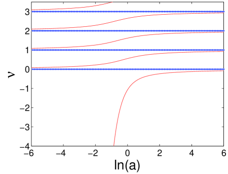
Figure 1: Energy spectrum $\nu$ as function of ${\rm ln}(a)$. The unmarked red curves are for those solutions affected by the scattering potential, and the marked blue horizontal lines are for asymptotic values as ${\rm ln}(a)\to\pm\infty$.

We note the scattering length is nonnegative verhaar . The results of $\nu$ as function of ${\rm ln}(a)$ are shown in Fig. 1. We find that the energy spectrum behaves like that in a 1D and 3D trap: (1) the energy is a smooth and monotonic function of the scattering length, and (2) the energy is bounded except for the ground state.

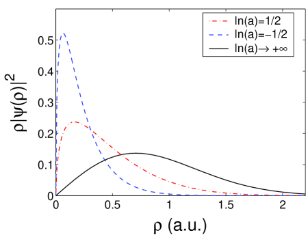
Figure 2: The radial density distribution of the ground state.

The radial densities $\rho|\psi(\rho)|^{2}$ of the ground state is shown in Fig. 2 for chosen scattering lengths ${\rm ln}(a)=\pm 1/2$ and ${\rm ln}(a)\to+\infty$. We can see that the atoms tend to approach each other as ${\rm ln}(a)$ decreases. In addition, we note that the derivative diverges at $\rho=0$ for ${\rm ln}(a)=\pm 1/2$ which originates from the scattering potential. While for ${\rm ln}(a)\to+\infty$ it has a finite derivative corresponding to the non-interacting case. This is because in this limit, the effective coupling strength $g_{\rm 2D}\simeq-2\pi/{\rm ln}(a)$ approaches 0 calarco .

After obtaining the spectrum, we are able to compute the entanglement. We adopt von Neumann entropy as our pure state entanglement measure Ni . We are interested in the pair entanglement for pure states with c.m. motion being the ground state of the trap. The total wave function is

$$\Psi_{0\nu}(\varrho,\rho)={\Gamma(-\nu)\over\pi\sqrt{\zeta(2,-\nu)}}e^{-{\varrho^{2}+\rho^{2}\over 2}}U(-\nu,1,\rho^{2}).$$ (9)

First, we briefly review the method in Ref. law which is also applicable to our case. Since $\varrho^{2}=(\rho_{1}^{2}+\rho_{2}^{2}+2\rho_{1}\rho_{2}{\rm cos}(\varphi_{1}-\varphi_{2}))/2$ and $\rho^{2}=(\rho_{1}^{2}+\rho_{2}^{2}-2\rho_{1}\rho_{2}{\rm cos}(\varphi_{1}-\varphi_{2}))/2$, we can expand the total wave function as $\Psi_{0\nu}(\varrho,\rho)=\sum_{m}A_{m}(\rho_{1},\rho_{2})e^{im(\varphi_{1}-\varphi_{2})}/(\rho_{1}\rho_{2})$. $A_{m}(\rho_{1},\rho_{2})$ can be further written in the Schmidt form $A_{m}(\rho_{1},\rho_{2})=\sum_{s}\kappa_{m,s}\chi_{s}^{(m)}(\rho_{1})\chi_{s}^{(m)}(\rho_{2})$ with

$$\int_{0}^{+\infty}A_{m}(\rho_{1},\rho_{2})\chi_{s}^{(m)}(\rho_{2})d\rho_{2}=\kappa_{m,s}\chi_{s}^{(m)}(\rho_{1}).$$ (10)

Thus, the total wave function can also be written in the Schmidt form

$$\Psi_{0\nu}(\varrho,\rho)=\sum_{m,s}\kappa_{m,s}\left[{\chi_{s}^{(m)}(\rho_{1})\over\rho_{1}}e^{im\varphi_{1}}\right]\left[{\chi_{s}^{(m)}(\rho_{2})\over\rho_{2}}e^{im\varphi_{2}}\right]^{*}.$$ (11)

The entropic entanglement can then be calculated from the Schmidt coefficients as $\mathcal{E}=-\sum_{m,s}\kappa_{m,s}^{2}{\rm ln}(\kappa_{m,s}^{2})$.

Here we use an alternative method to calculate the entanglement. We find the following decomposition in the single particle basis

$$\Psi_{0\nu}(\vec{\rho}_{1},\vec{\rho}_{2})=\sum_{\vec{m},\vec{n}}C_{\vec{m}\vec{n}}\phi_{\vec{m}}(\vec{\rho}_{1})\phi_{\vec{n}}(\vec{\rho}_{2})$$ (12)

$$= {2\over\pi\sqrt{\zeta(2,-\nu)}}\sum_{\vec{m},\vec{n}}{1\over 2\nu-\sum_{j}(m_{j}+n_{j})}\prod_{j}{1+(-1)^{m_{j}+n_{j}}\over 2}$$

$$\times(-1)^{m_{j}-n_{j}\over 2}{\Gamma\left({m_{j}+n_{j}+1\over 2}\right)\over\sqrt{m_{j}!n_{j}!}}\phi_{m_{j}}(\rho_{1j})\phi_{n_{j}}(\rho_{2j}),$$

where $j=\{x,y\}$, ${\vec{m}}=(m_{x},m_{y})$ and ${\vec{n}}=(n_{x},n_{y})$. $\rho_{kj}$ is the $j$-th component of the position vector $\vec{\rho}_{k}$ for the $k$-th atom in cartesian coordinate, e.g., $\rho_{1x}=x_{1}$. $\phi_{\vec{m}}(\vec{\rho})$ is the 2D harmonic orbital again in cartesian coordinate. This decomposition can be proved straightforwardly and its validity holds as long as the c.m. motion is in the ground state of the trap. We then diagonalize the expansion coefficient matrix $[C_{\vec{m}\vec{n}}]$ and obtain $U^{\dagger}CU=D$, where $D$ is a diagonal matrix with diagonal elements $\lambda_{n}$ satisfying $\sum_{n}\lambda_{n}^{2}=1$. The von Neumann entropy is then given by $\mathcal{E}=-\sum_{n}\lambda_{n}^{2}{\rm ln}(\lambda_{n}^{2})$. The calculated entropy is shown in Fig. 3 where the (red) decreasing curve is for the ground state and the lower (blue) and upper (blue) increasing curves are for the first and second excited state, respectively. We find that the tendency of the curves remains essentially the same as in the 3D case law . In addition, the result is in a qualitative agreement with that from a cylindrical trap with an aspect ratio $\eta=\omega_{\perp}\ll\omega_{z}$ bof . It is interesting to make a quantitative comparison between a 2D and quasi-2D geometry. To do this, we note that, in the quasi-2D case, an effective scattering length is given by olshanii ; shl

$$a_{\rm eff}=2.092a_{z}{\rm exp}\left(-\sqrt{\pi\over 2}{a_{z}\over a_{3D}}\right),$$ (13)

where $a_{3D}$ is the original 3D scattering length and $a_{z}=\sqrt{\hbar/(m\omega_{z})}$ is the length scale along the tightly confined $z$-axis. Transforming Eq. (13) into the unit that is adopted in the current paper, it reads

$${\rm ln}{a_{\rm eff}\over a_{\perp}}={\rm ln}{2.092\over\sqrt{\eta}}-\sqrt{\pi\over 2}{a_{z}\over a_{3D}}.$$ (14)

Our comparison with $\eta=20$ is also shown in Fig. 3 where data points with diamonds (circles) are for the first (second) excited state. We do not make comparison for the ground state nr . We can see that the two results agree well with each other except for the critical region where $a_{3D}\sim\pm\infty$ and the corresponding effective scattering length is ${\rm ln}a_{\rm eff}^{(cr)}={\rm ln}(2.092/\sqrt{\eta})$ as from Eq. (14). For $\eta=20$, ${\rm ln}a_{\rm eff}^{(cr)}\simeq-0.76$. The 2D results vary more slowly than the quasi-2D results around the critical region. The discrepancy is expected since in deriving the effective scattering length in Eq. (13), there is no trapping potential in the transverse direction. While in our study, the existence of such a transverse trapping potential may have an effect on the scattering problem.

To better understand the entanglement properties, we give an example for the eigenvalues and eigenfunctions. We randomly choose a scattering length ${\rm ln}(a)=-0.5359$ and the corresponding results are shown in Figs. 4 and 5, respectively.

In Fig. 4, we show the first 20 eigenvalues for the ground state. Using a fitting curve $\lambda_{n}=\alpha n^{\beta}$, we obtain $\alpha\simeq 0.7$ and $\beta\simeq-0.9$. This slow decrease is expected since the eigenfunction $\Psi_{0\nu}(\vec{\rho}_{1},\vec{\rho}_{2})$ is singular at the origin which can only be removed by a regularized pseudopotential. On the other hand, the entanglement is convergent which can be seen from the power law relation of the eigenvalues and further confirmed by our numerical results. In Fig. 5, we show the eigenfunctions (Schmidt orbitals) for four different eigenvalues for the ground state. The Schmidt orbital $\tilde{\phi}(\vec{\rho})$ is related to the harmonic basis by a unitary transformation, i.e., $\tilde{\phi}(\vec{\rho})\equiv U^{\dagger}\phi(\vec{\rho})$. The ${\vec{p}}$-th component of $\tilde{\phi}(\vec{\rho})$ can be written as $\tilde{\phi}_{\vec{p}}(\vec{\rho})=\sum_{\vec{m}}U^{\dagger}_{\vec{p}\vec{m}}\phi_{\vec{m}}(\vec{\rho})$. Compared to harmonic orbitals, these orbitals experience deformation due to the interaction. On the other hand, the symmetry of the orbitals is still preserved due to the isotropic interaction. For example, if we rotate the orbital in Fig. 5(b) by $90^{o}$, we obtain another eigenstate which is degenerate to it. These two eigenstates correspond to the second and third eigenvalue in Fig. 4.

Two limiting cases, i.e., ${\rm ln}(a)\to\pm\infty$, deserve a simple discussion. When ${\rm ln}(a)\to+\infty$, we have already mentioned before that it corresponds to the non-interacting regime. While for ${\rm ln}(a)\to-\infty$, we can see that the entanglement goes without limit. We identify it as the bound state regime, where the binding energy is calculated from Eq. (8) with the result $E_{b}\to-2\nu\simeq 1/a^{2}$ as $\nu\to-\infty$. The size of the bound state is on the order of $a$, thus a vanishingly small cross section in this regime. This is a quite general conclusion in the scattering theory. At low energy, the scattering amplitude for an $l$-wave is given by llbook

$$f_{l}\sim{(kb)^{2l}\over-a_{l}^{-1}-r_{l}k^{2}/2-i(kb)^{2l}k},$$ (15)

where $b$ is a constant only depending on the scattering potential and $r_{l}$ is the effective range. The bound state can be obtained from the pole of $f_{l}$. For low energy ($k\to 0$) s-wave scattering ($l=0$), it gives $k=i/a$. The corresponding wave length $\lambda\sim|1/k|=a$, thus a size of $a$. The bound state energy is $E_{b}=|k^{2}|=1/a^{2}$. Both analysis are in agreement with our results.

In conclusion, we have carried out the calculation for the entanglement between two interacting bosons in a 2D isotropic harmonic trap. The $s$-wave scattering is modelled by the well-known 2D regularized pseudopotential. By decomposing the wave function into single particle basis, we have shown the dependency of the pair entanglement on the scattering length. In addition, we have analyzed the Schmidt mode (natural orbit) of the system. Our current study only focuses on pure states, the more general entanglement properties with a temperature dependence will be an open question for future investigations notes1 . With the possible realization of a 2D few-body quantum system in the future and the controllability of the scattering length through Feshbach resonance, we hope our results could be helpful to the study of quantum information and communication in low dimensional systems.

This work is supported by grants with NSF.

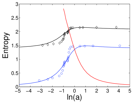
Figure 3: Von Neumann entropy as function of the scattering length. The (red) decreasing curve is for the ground state. The lower (blue) and upper (black) of the two increasing curves are for the first and second excited state (both perturbed by interaction) in the relative motion. The c.m. motion is always assumed in the ground state of the trap. Data points with circles (blue) and diamonds (black) are from quasi-2D calculations with $\eta=20$ and an effective scattering length of Eq. (13). See text for details.

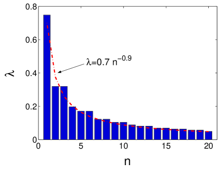
Figure 4: The first 20 eigenvalues $\lambda_{n}$ in descending order for the ground state with ${\rm ln}(a)=-0.5359$. The (red) dashed dotted line is an exponential fit.

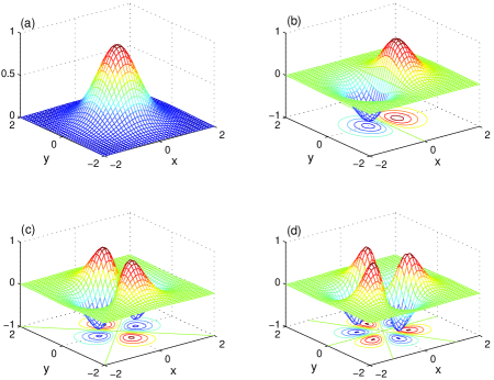
Figure 5: Several Schmidt orbitals for the ground state with ${\rm ln}(a)=-0.5359$. From (a)$\to$(d), the corresponding eigenvalues are 0.7408,0.3164,0.1686, and 0.1029, respectively.

References

- (1) Greiner M., Mandel O., Esslinger T., Hänsch T. W., and Bloch I., Nature 415, (2002) 39.
- (2) Schrader D., Dotsenko I., Khudaverdyan M., Miroshnychenko Y., Rauschenbeutel A., and Meschede D., Phys. Rev. Lett. 93, (2004) 150501.
- (3) Maunz P., Puppe T., Schuster I., Syassen N., Pinkse P. W. H., and Rempe G., Nature 428, (2004) 50.
- (4) Paredes B., Widera A., Murg V., Mandel O., Fölling S., Cirac I., Shlyapnikov G., Hansch T. W., and Bloch I., Nature 429, (2004) 277.
- (5) Kinoshita T., Wenger T., and Weiss D., Science 305, (2004) 5687.
- (6) Kohl M., Stoeferle T., Guenter K., Koehl M., and Esslinger T., Phys. Rev. Lett. 94, (2005) 080403; Stoeferle T., Moritz H., Guenter K., Koehl M., and Esslinger T., Phys. Rev. Lett. 96, (2006) 030401.
- (7) Sheehy D. E. and Radzihovsky L., Phys. Rev. Lett. 95, (2005) 130401.
- (8) Orignac E. and Citro R., Phys. Rev. A 73, (2006) 063611.
- (9) Petrov D.S., Holzmann M., and Shlyapnikov G. V., Phys. Rev. Lett 84, (2000) 2551; Fedichev P. O., Bijlsma M. J., and Zoller P., Phys. Rev. Lett. 92, (2004) 080401.
- (10) Astrakharchik G. E., Boronat J., Kurbakov I. L., and Lozovik Yu. E., Phys. Rev. Lett. 98, (2007) 060405.
- (11) Olshanii M., Phys. Rev. Lett. 81, (1998) 938.
- (12) Girardeau M., J. Math. Phys. (N.Y.) 1, (1960) 516.
- (13) Nielsen M. A. and Chuang I. S., Quantum computation and quantum information, Cambridge University Press (2000).
- (14) Sun B., Zhou D. L., and You L., Phys. Rev. A 73, (2006) 012336.
- (15) Wang J., Law C. K., and Chu M.-C., Phys. Rev. A 72, (2005) 022346.
- (16) Sun B., You L., and Zhou D. L., Phys. Rev. A 75, (2007) 012332.
- (17) Pricoupenko L. and Olshanii M., J. Phys. B: At. Mol. Opt. Phys. 40, (2007) 2065.
- (18) Bolda E. L., Tiesinga E., and Julienne P. S., Phys. Rev. A 66, (2002) 013403.
- (19) Busch T., Englert B.-G., Rzazewski K., and Wilkens M., Found. Phys. 28, (1998) 549.
- (20) Arfken G., Mathematical Methods for Physicists, 3rd Ed., Academic Press, Inc., (1987).
- (21) For , we can use and integrate on both sides to obtain . Then can be obtained by using the Wronskian of two confluent hypergeometric functions . Comparing both sides, we immediately obtain Eq. (7).
- (22) Verhaar B. J., Eijnde J. P. H. W. van den, Voermans M. A. J., and Schaffrath M. M. J., J. Phys. A 17, (1984) 595.
- (23) Idziaszek Z. and Calarco T., Phys. Rev. A 74, (2006) 022712.
- (24) Petrov D. S. and Shlyapnikov G. V., Phys. Rev. A 64, (2001) 012706.
- (25) The ground state entanglement in a quasi-2D geometry is computationly intensive. Even for a moderate scattering length, it requires much more basis for the expansion than the 2D case in order to achieve convergence. Due to this numerical difficulty, the ground state entanglement is not given in Ref. bof and as a result, a comparison is not carried out.
- (26) Landau L. D. and Lifschitz E. M., Vol. 3 Quantum mechanics, Nonrelativistic theory (3ed., Pergamon, 1991).
- (27) For the thermal entanglement which is related to mixed states in general, we can use negativity as entanglement measure werner . Different from pure state calculation which only need the reduced density matrix, the calculation of negativity need the full two-body density matrix. This is a computationally demanding task due to the very large Hilbert space.
- (28) Vidal G. and Werner R. F., Phys. Rev. A 65, (2002) 032314.