Decoherence in a dynamical quantum phase transition

Abstract

Motivated by the similarity between adiabatic quantum algorithms and quantum phase transitions, we study the impact of decoherence on the sweep through a second-order quantum phase transition for the prototypical example of the Ising chain in a transverse field and compare it to the adiabatic version of Grovers search algorithm, which displays a first order quantum phase transition. For site-independent and site-dependent coupling strengths as well as different operator couplings, the results show that (in contrast to first-order transitions) the impact of decoherence caused by a weak coupling to a rather general environment increases with system size (i.e., number of spins/qubits). This might limit the scalability of the corresponding adiabatic quantum algorithm.

I Introduction

I.1 Quantum Phase Transitions

In contrast to thermal phase transitions occurring when the strength of the thermal fluctuations reaches a certain threshold, during recent years, a different class of phase transitions has attracted the attention of physicists, namely transitions taking place at zero temperature sachdev . An analytic non-thermal control parameter such as pressure, magnetic field, or chemical composition is varied to access the transition point. Despite the analytic form of the order parameter, the ground state of a system changes non-analytically. There, order is changed solely by quantum fluctuations, hence the name quantum phase transition (QPT). Let us consider a quantum system (at zero temperature) described by the Hamiltonian $H$ depending on some external parameter $g$. At a certain critical value of this parameter $g_{c}$, the system is supposed to undergo a phase transition, i.e., the ground state $\left|\Psi_{<}(g)\right>$ of $H(g)$ for $g<g_{c}$ is strongly different from the ground state $\left|\Psi_{>}(g)\right>$ of $H(g)$ for $g>g_{c}$. For example, $\left|\Psi_{<}(g)\right>$ and $\left|\Psi_{>}(g)\right>$ could have different global/topological properties (such as magnetization) in the thermodynamic limit.

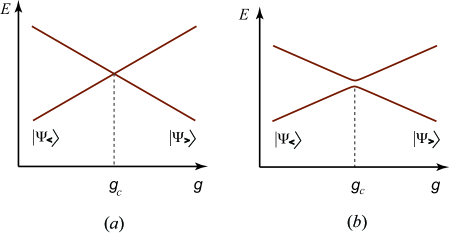
Figure 1: (Color Online) Sketch of the lowest eigenvalues of a Hamiltonian $H(g)$ as a function of some external parameter $g$ for a first order QPT. At the critical point $g=g_{c}$, the ground state changes from $\left|\Psi_{<}(g)\right>$ to $\left|\Psi_{>}(g)\right>$. $(a)$ A level-crossing. $(b)$ An avoided level-crossing.

Therefore, a quantum phase transition can also be defined as a non-analyticity of the ground state properties of the system as a function of the control parameter. If this singularity arises from a simple level crossing in the ground state, see Fig. (1)-$(a)$, then we have a first-order quantum phase transition. The situation is different for continuous transitions, where a higher-order discontinuity in the ground state energy occurs. Typically, for any finite-size system a transition will be rounded into a crossover, this is nothing but an avoided level-crossing in the ground state, see Fig. (1)-$(b)$. Continuous transitions can usually be characterized by an order parameter which is a quantity that is zero in one phase (the disordered) and non-zero and possibly non-unique in the other (the ordered) phase. If the critical point is approached, the spatial correlations of the order parameter fluctuations become long-ranged. Close to the critical point the correlation length $\Upsilon$ diverges as $\Upsilon^{-1}\propto\Lambda|g-g_{c}|^{\mathfrak{d}}\,,$ where $\mathfrak{d}$ is a critical exponent and $\Lambda$ is an inverse length scale of the order of the inverse lattice spacing. Let $\Delta$ denote the smallest energy excitation gap above the ground state. In most cases, it has been found sachdev that as $g$ approaches $g_{c}$, $\Delta$ vanishes as $\Delta\propto\Upsilon^{-z}\propto\Lambda^{z}|g-g_{c}|^{\mathfrak{d}z}\,,$ where $z$ is the dynamic critical exponent. This poses a scalability problem for adiabatic ground state preparation schemes (see below), as these require a nonvanishing energy gap $\Delta$.

I.2 Adiabatic Quantum Computation

Unfortunately, the actual realization of usual sequential quantum algorithms (where a sequence of quantum gates is applied to some initial quantum state, see, e.g., nielsen ) goes along with the problem that errors accumulate over many operations and the resulting decoherence tends to destroy the fragile quantum features needed for the computation. Therefore, adiabatic quantum algorithms have been suggested farhi-2000 , where the solution to a problem is encoded in the (unknown) ground state of a (known) Hamiltonian. Since there is evidence that, in adiabatic quantum computing the ground state is more robust against decoherence – the ground state cannot decay and phase errors do not play any role, i.e., errors can only result from excitations childs_robust ; sarandy_open – this scheme offers fundamental advantages compared to sequential quantum algorithms – a sufficiently cold reservoir provided. Suppose we have to solve a problem that may be reformulated as preparing a quantum system in the ground state of a Hamiltonian $H_{\rm f}$ . The adiabatic theorem messiah then provides a straightforward method to solve this problem: Prepare the quantum system in the (known and easy-to-prepare) ground state of another Hamiltonian $H_{0}$. Apply $H_{0}$ on the system and slowly modify it to $H_{\rm f}$. The adiabatic theorem ensures for a non-vanishing time-dependent energy gap that if this has been done slowly enough, the system will end up in a state close to the ground state of $H_{\rm f}$. Therefore, a measurement of the final state will yield a solution of the problem with high probability.

Furthermore, adiabatic quantum algorithms display a remarkable similarity with sweeps through quantum phase transitions latorre ; gernot . For all interesting systems discussed later in this article, adiabatic quantum computation inherently brings the quantum system near to a point which is similar to the critical point in a quantum phase transition. As an example for the deformation of the Hamiltonian, one can consider the linear interpolation path between these two Hamiltonians

$$H(g)=[1-g(t)]H_{0}+g(t)H_{\rm f}\,,$$ (1)

with $g(0)=0$ and $g(T)=1$, where $T$ is the total evolution time or the run-time of the algorithm. We prepare the ground state of $H_{0}$ at time $t=0$, and then the state evolves from $t=0$ to $T$ according to the Schrödinger equation. At time $T$, we measure the state. According to the adiabatic theorem, if there is a nonzero gap between the ground state and the first excited state of $H(g)$ for all $g\in[0,1]$ then the success probability of the algorithm approaches 1 in the limit $T\to\infty$. How large $T$ should actually be is roughly given by sarandy2004 (for a more detailed discussion see, e.g. schaller2006b ; jansen2007a )

$$T\gg\frac{\max_{g\in[0,1]}\left|\left<1,g\right|\frac{dH(g)}{dg}\left|0,g\right>\right|}{\min_{g\in[0,1]}\left[E_{1}(g)-E_{0}(g)\right]^{2}}\,,$$ (2)

where $E_{0}(g)$ is the lowest eigenvalue of $H(g)$, $E_{1}(g)$ is the second-lowest eigenvalue, and $\left|0,g\right>$ and $\left|1,g\right>$ are the corresponding eigenstates, respectively. Somewhere on the way from the simple initial configuration $H_{0}$ to the unknown solution of some problem encoded in $H_{\rm f}$, there is typically a critical point which bears strong similarities to a quantum phase transition. At this critical point the fundamental gap (which is sufficiently large initially and finally) becomes very small, see, e.g., Fig. (2). Near the position of the minimum gap, the ground state will change more drastically than in other time intervals of the interpolation. In the continuum limit, one would generally expect that the minimum value of the fundamental gap in adiabatic computation will vanish identically and that the ground state will change non-analytically at the critical point. This is similar to what happens in quantum phase transition when $g$ approaches $g_{c}$. Based on this similarity, it seems gernot that adiabatic quantum algorithms corresponding to second-order quantum phase transitions should be advantageous compared to isolated avoided level crossings (which are analogous to first-order transitions). A brief review of this idea comes in the following section.

II Examples

II.1 First-Order Transition – Grovers Algorithm

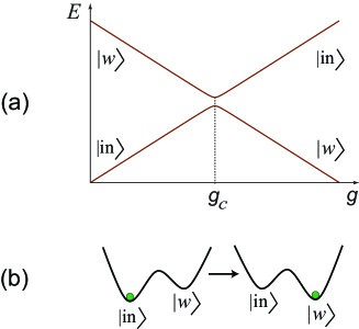
Figure 2: (Color Online) Sketch of the two lowest energy eigenvalues of the Grover Hamiltonian (a). In the continuum limit, this corresponds to the time evolution of the energy landscape for a first-order transition (b). The green dot in the energy landscape denotes the ground state.

An adiabatic version of Grovers algorithm roland is defined by the Hamiltonian

$$H(g)=(1-g)H_{0}+gH_{\rm{f}}\,,$$ (3)

where the initial Hamiltonian is given by $H_{0}=\mbox{\boldmath$1$}-\left|{\rm in}\right>\left<{\rm in}\right|$ with the initial superposition state $\left|{\rm in}\right>=\sum_{x=0}^{D-1}\left|x\right>/\sqrt{D}$ and $D\equiv 2^{N}$ denotes the dimension of the Hilbert space for $N$ qubits. The final Hamiltonian reads $H_{\rm f}=\mbox{\boldmath$1$}-\left|w\right>\left<w\right|$, where $\left|w\right>$ denotes the marked state. In this case, the commutator is very small $[H_{0},H_{\rm f}]=(\left|{\rm in}\right>\left<w\right|-\left|w\right>\left<{\rm in}\right|)/\sqrt{D}$ and one can nearly diagonalize both Hamiltonians simultaneously and the $g$-dependent spectrum will consist of nearly straight lines – except near $g_{c}=1/2$, where we have an avoided level-crossing, see Fig. (2). In the continuum limit of $N\to\infty$, this corresponds to a first-order quantum phase transition from $\left|\rm{in}\right>=\left|\rightarrow\cdots\rightarrow\right>$ to $\left|w\right>=\left|\uparrow\downarrow\cdots\uparrow\downarrow\downarrow\right>$, for example, at the critical point $g_{c}=1/2$. Such a first-order transition is characterized by an abrupt change of the ground state – $\left|\rm{in}\right>$ for $g<g_{c}$ and $\left|w\right>$ for $g>g_{c}$ – resulting in a discontinuity of a corresponding order parameter, see Fig. (3),

$$\left<\psi_{0}(g)\right|\frac{dH}{dg}\left|\psi_{0}(g)\right>=\frac{dE_{0}}{dg}\,.$$ (4)

In contrast to the conventional order parameters, for linear interpolations in Eqn. (3) the operator $dH/dg$ treats both phases symmetrically. Since $[H_{I},H_{F}]\neq 0$ (for nontrivial systems), $dH/dg$ is off-diagonal in either phase and thereby plays an equivalent role such as e.g. magnetization.

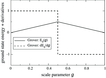
Figure 3: The ground-state energy of the Grover Hamiltonian and its first-order derivative. The discontinuity in the first-order derivative of the ground state suggests the first-order quantum phase transition in adiabatic quantum search algorithm.

First-order quantum phase transitions are typically associated with an energy landscape pictured in Fig. (2), where the two competing ground states are separated by an energy barrier throughout the interpolation. In order to stay in the ground state, the system has to tunnel through the barrier between the initial ground state $\left|\rm{in}\right>$ and the final ground state $\left|w\right>$ during the quantum phase transition. The natural increase of the strength of the barrier with the system size $N$ yields to the tunneling time which scales exponentially with the system size. Specifically, the optimal run-time for the adiabatic search algorithm behaves as $T={\cal O}(\sqrt{D})={\cal O}\left(2^{N/2}\right)$ roland . The observation that this first order QPT is associated with an exponentially small energy gap right at the avoided crossing can be generalized schuetzhold2008a to local Hamiltonians: The two-dimensional subspace of the avoided crossing is spanned by the eigenstates $\left|w_{<}(g)\right>$ and $\left|w_{>}(g)\right>$ that become degenerate at $g=g_{c}$. Due to their macroscopic distinguishability, the overlap between these states is exponentially small, which for local Hamiltonians also transfers to the matrix element $\left<w_{<}(g_{c})\right|H(g_{c})\left|w_{>}(g_{c})\right>={\cal O}\left(\exp\{{-D}\}\right)$. Consequently, one can conclude from the eigenvalues of $H(g)$ in this two-dimensional subspacethat also the minimum energy gap will become exponentially small in this case.

Therefore, the abrupt change of the ground state and the energy barrier between the initial and final ground states suggest that the first-order transitions are not the best choice for the realization of adiabatic quantum algorithms gernot . Thus, it would be relevant to study higher-order quantum phase transitions for this purpose.

II.2 Second-Order Transition – Ising Model

The one-dimensional quantum Ising model is one of the two paradigmatic examples sachdev for second-order quantum phase transition (the other is Bose-Hubbard model). Of these two, only the former model is exactly solvable bunder ; sachdev – the Ising model in a transverse field is a special case of the XY model (which can also be diagonalized completely). This model has been employed in the study of quantum phase transitions and percolation theory sachdev , spin glasses sachdev ; fischer , as well as quantum annealing chakrabarti ; santoro ; kadowaki etc. Although its Hamiltonian is quite simple, the Ising model is rich enough to display most of the basic phenomena near quantum critical points. Furthermore, the transverse Ising model can also be used to study the order-disorder transitions at zero temperature driven by quantum fluctuations sachdev ; chakrabarti . Finally, two-dimensional generalizations of the Ising model can be mapped onto certain adiabatic quantum algorithms (see, e.g., dwave ). However, due to the evanescent excitation energies, such a phase transition is rather vulnerable to decoherence, which must be taken into account deco .

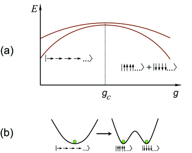
Figure 4: (Color Online) Sketch of the two lowest energy levels of the Ising Hamiltonian (left) given in Eqn. (5) and the time evolution of the energy landscape for a second-order transition (right). A symmetry-breaking transition corresponds to the deformation of the energy landscape. The green dot in the energy landscape denotes the ground state.

The one-dimensional transverse Ising chain of $N$ spins exhibits a time-dependent nearest-neighbor interaction $g(t)$ plus transverse field $B(t)=1-g(t)$

$${H}_{\rm{sys}}(t)=-\sum_{j=1}^{N}\left\{[1-g(t)]\,\sigma^{x}_{j}+g(t)\,\sigma^{z}_{j}\sigma^{z}_{j+1}\right\}\,,$$ (5)

where ${\mbox{\boldmath$\sigma$}}_{j}=(\sigma^{x}_{j},\sigma^{y}_{j},\sigma^{z}_{j})$ are the spin-1/2 Pauli matrices acting on the $j$th qubit and periodic boundary conditions ${\mbox{\boldmath$\sigma$}}_{N+1}={\mbox{\boldmath$\sigma$}}_{1}$ are imposed. This Hamiltonian is invariant under a global 180-degree rotation around the $\sigma_{j}^{x}$-axes (bit flip) which transforms all qubits according to $\sigma_{j}^{z}\to-\sigma_{j}^{z}$. Choosing $g(0)=0$ and $g(T)=1$ where $T$ is the evolution time, the quantum system evolves from the unique paramagnetic state $\left|\rm{in}\right>=\left|\rightarrow\rightarrow\rightarrow\dots\right>$ through a second-order quantum phase transition (see figure 5) at $g_{\rm cr}=1/2\,\,$ to the symmetrized combination in the two-fold degenerate ferromagnetic subspace, see also Fig. 4.

$$\left|w\right>=\frac{\left|\uparrow\uparrow\uparrow\dots\right>+\left|\downarrow\downarrow\downarrow\dots\right>}{\sqrt{2}}\,.$$ (6)

At the critical point $g_{\rm cr}$ the excitation gap vanishes (in the thermodynamic limit $N\to\infty$) and the response time diverges. As a result, driving the system through its quantum critical point at a finite sweep rate entails interesting non-equilibrium phenomena such as the creation of topological defects, i.e., kinks dziarmaga .

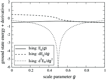
Figure 5: The ground-state energy for the Ising model and its first and second derivatives. The discontinuity in the second-order derivative of the ground state suggests a second-order quantum phase transition.

Since the initial ground state $\left|\rm{in}\right>$ reflects the bit-flip invariance of the Hamiltonian (5) whereas the final ground state subspace $\left|\uparrow\ldots\uparrow\right>$ and $\left|\downarrow\ldots\downarrow\right>$ breaks this symmetry, we have a symmetry-breaking quantum phase transition. Typically, such a symmetry-breaking change of the ground state corresponds to a second-order phase transition gernot . For such a transition, the ground state changes continuously and the energy barrier observed in first-order transitions is absent: Initially, there is a unique ground state but at the critical point, this ground state splits up into two degenerate ground states which are the mirror image of each other. Therefore, the ground state does not change abruptly in this situation and the system does not need to tunnel through a barrier in order to stay in the ground state, see Figs. (4b). Consequently, we expect that in this case, a closed quantum system should find its way from the initial to the final ground state easier. This expectation is confirmed in the following sections of this article: Since the minimum gap behaves as ${\cal O}(1/N)$, the optimal run-time in order to stay in the ground state scales polynomially for the Ising model.

II.3 Mixed Case

Looking at Fig. (4), it seems that a symmetry-breaking quantum phase transition typically corresponds to a second-order phase transition, but there are counter-examples: Consider more complicated energy landscape gernot-symmetry in Fig. (6).

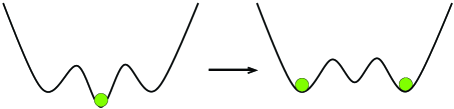
Figure 6: (Color Online) Sketch of the time evolution of the energy landscape for a symmetry-breaking quantum phase transition which is of first order. The green dot denotes the ground state.

In spite of the mirror symmetry of the energy landscape, there is a tunneling barrier throughout the interpolation. An analytic example for a symmetry-breaking first-order transition gernot-symmetry is given by a combination of the initial Hamiltonian from the Grover problem with the final Hamiltonian of the Ising model

$$H_{0}=\mbox{\boldmath$1$}-\left|{\rm in}\right>\left<{\rm in}\right|\quad,\quad H_{\rm f}=\frac{1}{2}\sum_{j=1}^{N}\left(\mbox{\boldmath$1$}-\sigma_{j}^{z}\sigma_{j+1}^{z}\right)\,,$$ (7)

where $H_{\rm f}$ has been shifted and scaled in order to preserve the positive definiteness. Even though this Hamiltonian possesses the same bit-flip symmetry as the Ising model, its level structure displays an avoided-level crossing at the critical point, i.e., it corresponds to a first-order phase transition with a jump between the initial and the final ground state(s), see Fig. (7).

It can also be shown analytically that the fundamental gap of the combined Hamiltonian $H(g)=(1-g)H_{0}+gH_{\rm f}$ vanishes exponentially with the system size, i.e. the number of qubits, see, e.g., farhi0512159 ; zindaric-NP .

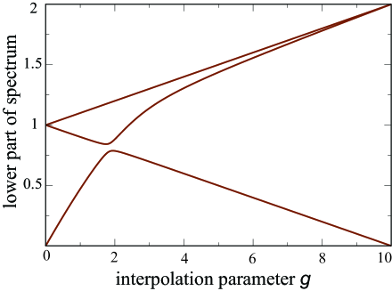
Figure 7: (Color Online) Sketch of the lowest eigenvalues of the Hamiltonian (7). One can clearly see that the spectrum displays an avoided-level crossing at the critical point – thus corresponding to a first-order transition gernot-symmetry .

III Decoherence in the Adiabatic Limit

In all of the above examples, we have seen that at the critical point, at least some energy levels become arbitrarily close and thus, the response times diverge (in the continuum limit). Consequently, during the sweep through such a phase transition by means of a time-dependent external parameter, small external perturbations or internal fluctuations become strongly amplified – leading to many interesting effects, see, e.g., group_phase0 ; group_phase1 ; vidal ; zurek ; damski ; sengupta ; fazio . One of them is the anomalously high susceptibility to decoherence (see also fubini ): Due to the convergence of the energy levels at the critical point, even low-energy modes of the environment may cause excitations and thus perturb the system. Based on the similarity between the quantum adiabatic algorithms and critical phenomena, we have argued that adiabatic quantum algorithms corresponding to the higher-order quantum phase transitions should be advantageous in comparison to those of first order for closed quantum systems. The present paper aims at generalizations to these findings when the impact of decoherence is considered.

In order to study the impact of decoherence, we consider an open system described by the total Hamiltonian ${H(t)}$ which can be split up into that of the closed system ${H}_{\rm{sys}}$ and the bath ${H}_{\rm{bath}}$ acting on independent Hilbert spaces ${\mathcal{H}}_{\rm{sys}}\otimes{\mathcal{H}}_{\rm{bath}}={\mathcal{H}}$

$${H}(t)\,=\,{H}_{\rm{sys}}(t)+{H}_{\rm{bath}}+\lambda\,{H}_{\rm{int}}\,,$$ (8)

plus an interaction $\lambda\,{H}_{\rm{int}}$ between the two, which is supposed to be weak $\lambda\ll 1$ in the sense that it does not perturb the state of the system drastically. Note that the change of the bath caused by the interaction need not be small. To describe the evolution of the combined quantum state $\left|\Phi(t)\right>\in{\mathcal{H}}$, we expand it using the instantaneous system energy eigenbasis ${H}_{\rm{sys}}(t)\left|\psi_{s}(t)\right>=E_{s}(t)\left|\psi_{s}(t)\right>$, via

$$\left|\Phi(t)\right>=\sum_{s}a_{s}(t)\left|\psi_{s}(t)\right>\otimes\left|\alpha_{s}(t)\right>\,,$$ (9)

where $a_{s}$ are the corresponding amplitudes and $\left|\alpha_{s}\right>\in{\mathcal{H}}_{\rm{bath}}$ denote the associated (normalized but not necessary orthogonal) states of the reservoir. Insertion of this expansion into the Schrödinger equation $i\left|\dot{\Phi}(t)\right>={H}(t)\left|\Phi(t)\right>$ yields ($\hbar=1$)

$$\frac{\partial}{\partial t}\left(a_{s}e^{-i\varphi_{s}}\right)=e^{-i\varphi_{s}}\sum_{r\neq s}a_{r}\,\times$$

$$\left(\frac{\left<\psi_{s}\right|\dot{H}_{\rm{sys}}\left|\psi_{r}\right>}{\Delta E_{sr}}\,\langle\alpha_{s}|\alpha_{r}\rangle-i\left<\alpha_{s}\right|\left<\psi_{s}\right|\lambda{H}_{\rm{int}}\left|\psi_{r}\right>\left|\alpha_{r}\right>\right)$$ (10)

with the energy gaps $\Delta E_{sr}(t)=E_{s}(t)-E_{r}(t)$ of the system and the total phase (including the Berry phase)

$$\varphi_{s}(t)=-\int_{0}^{t}dt^{\prime}\Big{\{}E_{s}(t^{\prime})+H_{\rm{bath}}^{ss}(t^{\prime})+\lambda H_{\rm{int}}^{ss}(t^{\prime})$$

$$\hskip 24.18501pt-i\langle\psi_{s}(t^{\prime})|\dot{\psi}_{s}(t^{\prime})\rangle-i\langle\alpha_{s}(t^{\prime})|\dot{\alpha}_{s}(t^{\prime})\rangle\Big{\}}$$ (11)

with the energy shift $H_{\rm{int}}^{sr}=\left<\alpha_{s}\right|\left<\psi_{s}\right|{H}_{\rm{int}}\left|\psi_{r}\right>\left|\alpha_{r}\right>$ , $H_{\rm{bath}}^{sr}=\left<\alpha_{s}\right|{H}_{\rm{bath}}\left|\alpha_{r}\right>$. Evidently, there are two contributions for transitions in the Hilbert space ${\mathcal{H}}_{\rm{sys}}$ of the system:

1. The first term on the right-hand side of Eqn. (III) describes the transitions caused by a non-adiabatic evolution sarandy2004 . Note, however, that the factor $\langle\alpha_{s}|\alpha_{r}\rangle$ and the additional phases in Eqn. (III) give rise to modifications in the adiabatic expansion.

2. The last term in Eqn. (III) directly corresponds to transitions caused by the interaction of the quantum system with its environment.

Since we are mainly interested in the impact of the coupling to the bath, we shall assume a perfectly adiabatic evolution of the system itself, i.e., without the coupling to the environment $\lambda=0$, the system would stay in its ground state. Thus, the only decoherence channel available is heating (i.e., excitations), the phase damping and decay channels, for example, play no major role here. Considering the adiabatic condition

$$\left<\psi_{s}\right|\dot{H}_{\rm{sys}}\left|\psi_{r}\right>\ll\left(\Delta E_{sr}\right)^{2}\,,$$ (12)

the first term in Eqn. (III) is negligible and the second one dominates. Starting in the system’s ground state $a_{0}(t=0)=1$, which is relevant for adiabatic quantum computation, the excitations $s>0$ caused by the weak interaction $\lambda H_{\rm{int}}$ with the bath

$$\mathfrak{A}_{s}\equiv a_{s}(T)\exp\{-i\varphi_{s}(T)\}$$ (13)

can be calculated via response theory, i.e., the solution of Eqn. (III) is to first order in $\lambda\ll 1$ given by

$$\mathfrak{A}_{s}\approx-i\int_{0}^{T}dt\,\,e^{i\Delta\varphi_{0s}}\left<\alpha_{s}\right|\left<\psi_{s}\right|\lambda H_{\rm{int}}\left|\psi_{0}\right>\left|\alpha_{0}\right>\,,$$ (14)

where $\Delta\varphi_{rs}=\varphi_{r}(t)-\varphi_{s}(t)$. This is rather a general result.

In the following, after a brief review of the impact of decoherence on the sweep through a first-order quantum phase transition markus in section IV, we study in section V the impact of decoherence due to a general reservoir for the quantum Ising chain in a transverse field, which is considered a prototypical example for a second-order quantum phase transition.

IV Decoherence in the Adiabatic Grover Search

Let us consider the Grover model (3) – weakly coupled to a bath, where we can assume the following expansion of the interaction Hamiltonian markus

$$\lambda H_{\rm{int}}=\lambda\sum_{j=1}^{N}\mbox{\boldmath$\sigma$}_{j}\cdot\mbox{\boldmath$A$}_{j}+\lambda^{2}\sum_{\ell,j=1}^{N}\mbox{\boldmath$\sigma$}_{\ell}\cdot\mbox{\boldmath$B$}_{\ell j}\cdot\mbox{\boldmath$\sigma$}_{j}+{\cal O}(\lambda^{3})\,,$$

where $\lambda\ll 1$ and $\mbox{\boldmath$\sigma$}_{j}(t)=(\sigma_{j}^{x}(t),\sigma_{j}^{y}(t),\sigma_{j}^{z}(t))$ is the vector of Pauli matrices in the interaction picture with the corresponding bath operators $\mbox{\boldmath$A$}_{j}(t)$ and $\mbox{\boldmath$B$}_{\ell j}(t)$, etc. Recalling the adiabatic version of Grovers search algorithm in Eqn. (3), at the beginning of the evolution the system has to be prepared in the ground state $\left|{\rm in}\right>=\sum_{x=0}^{D-1}\left|x\right>/\sqrt{D}$. This also requires that the initial full density operator can be initialized as a direct product

$$\varrho(0)=\varrho_{\rm{sys}}(0)\otimes\varrho_{\rm{bath}}(0)\,,$$ (16)

i.e., system and environment are not entangled at the beginning. Since in the weak-coupling limit the adiabaticity condition for the open system dynamics is still in leading order the same as for the closed system, similar to the discussions in the former section, one can assume perfect adiabatic evolution of the unperturbed system and hence only consider perturbations due to the interaction with the environment.

The spectrum of the Grovers Hamiltonian (3) consists of the ground state $\left|\psi_{0}(g)\right>$ and the first excited state $\left|\psi_{1}(g)\right>$, which come very close $\left(\Delta E_{\rm{min}}=1/\sqrt{D}\right)$ at $g_{c}=1/2$, whereas all other states $\left|\psi_{k>1}(g)\right>$ are degenerate and well separated from the ground state by an energy gap of order one. Since the temperature and hence the energies available in the environment must be much smaller than that gap of order one (in order to prepare the initial ground state), transitions from the ground state to these states $\left|\psi_{k>1}(g)\right>$ are exponentially suppressed. Thus, the final probability of the transitions to the first excited state markus

$$\left|\mathfrak{A}_{s}\right|^{2} \approx \lambda^{2}\sum_{\begin{subarray}{c}\ell,j=1\\ \mu,\nu=x,y,z\end{subarray}}^{N}\int_{0}^{T}dt_{1}\int_{0}^{T}dt_{2}\,\left<A_{\ell}^{\mu}(t_{1})A_{j}^{\nu}(t_{2})\right>\times$$ (17)

$$\times\,\left<w^{\perp}\right|\sigma_{\ell}^{\mu}(t_{1})\left|w\right>\left<w\right|\sigma_{j}^{\nu}(t_{2})\left|w^{\perp}\right>\,,$$

provides a good measure for the success probability which corresponds to $\left|\mathfrak{A}_{s}\right|^{2}\ll 1$. It can be shown markus that the contributions proportional to $\mbox{\boldmath$B$}_{\ell j}$ do not contribute to second order in $\lambda$. In this equation, $\left|w\right>$ denotes the marked state for Grovers problem, see Eqn. (3), and $\left|w^{\perp}\right>$ is the state orthogonal to $\left|w\right>$ in the subspace spanned by $\left|w\right>$ and $\left|\rm in\right>$. The expression (17) demonstrates that both system and reservoir properties affect the excitation amplitude. Of the system matrix elements $\left<w^{\perp}\right|\sigma_{j}^{\mu}(t)\left|w\right>$ only those with $\mu=x,z$ contribute (for large $D=2^{N}\ggg 1$, the $\mu=y$ term is suppressed by a factor $1/\sqrt{D}$)

$$\left<w^{\perp}\right|\sigma_{j}^{x}(t)\left|w\right>\approx-\,\frac{1-g(t)}{\sqrt{D}\Delta E(t)}\exp\left\{-i\int_{0}^{t}dt^{\prime}\Delta E(t^{\prime})\right\}\,,$$

for large $N$ and $\Delta E(t)=\sqrt{1-4g(t)[1-g(t)](1-1/D)}$. It is the same for $\left<w^{\perp}\right|\sigma_{j}^{z}(t)\left|w\right>$ apart from an additional sign $(-1)^{w_{j}+1}$, where $w_{j}$ is the $j$-th bit of $w$, i.e., $\left|w\right>$ is an eigenstate of the operators $\sigma_{j}^{z}$ with eigenvalues $(-1)^{w_{j}}$.

Assuming a stationary reservoir $\left[H_{\rm{bath}},\varrho_{\rm{bath}}\right]=0$ (which does not necessarily imply a bath in thermal equilibrium) allows for a Fourier decomposition of the bath correlation function

$$\left<A_{\ell}^{\mu}(t_{1})A_{j}^{\nu}(t_{2})\right>=\int_{-\infty}^{+\infty}d\omega\,e^{-i\omega(t_{1}-t_{2})}f_{\ell j}^{\mu\nu}(\omega)\,,$$ (19)

where $f_{\ell j}^{\mu\nu}(\omega)$ depends on the spectral distribution of the bath modes and the temperature, etc.

For example, for a bosonic bath in thermal equilibrium and coupling operators $A_{j}^{\mu}\propto\sum_{k}\left[h_{k}a_{k}+h_{k}^{*}a_{k}^{\dagger}\right]$ (as e.g., used in the spin-boson model) we would for an inverse bath temperature $\beta$ obtain a Fourier decomposition such as schaller2008a

$$f_{\ell j}^{\mu\nu}(\omega)\propto\frac{J(\left|\omega\right|)}{\left|1-e^{-\beta\omega}\right|}=\,J(\left|\omega\right|)\left[\frac{1}{e^{\beta\left|\omega\right|}-1}+\Theta(\omega)\right]\,,$$

where $\Theta(\omega)$ is the step function being 1 for $\omega>0$ and 0 for $\omega<0$. $J(\omega)$ denotes the spectral density, which is often parameterized as brandes2005a

$$J(\omega)=2\vartheta\omega_{\rm ph}^{1-\epsilon}\omega^{\epsilon}e^{-\omega/\omega_{\rm c}}\,,$$ (21)

where $0\leq\epsilon<1$ corresponds to the sub-ohmic, $\epsilon=1$ to the ohmic, and $\epsilon>1$ to the super-ohmic case.

Insertion of (IV) and (19) into Eqn. (17) yields

$$\hskip 28.45274pt\left|\mathfrak{A}_{s}\right|^{2} \approx \lambda^{2}\int d\omega\sum_{\ell,j=1}^{N}f_{\ell j}^{xx}(\omega)\,\times$$ (22)

$$\times\,\left|\int_{0}^{T}dt\,\,\frac{1-g(t)}{\sqrt{D}\Delta E(t)}\exp\left\{i\omega t+i\int_{0}^{t}dt^{\prime}\Delta E(t^{\prime})\right\}\right|^{2}$$

plus similar terms including $f_{\ell j}^{xz}$, $f_{\ell j}^{zx}$ and $f_{\ell j}^{zz}$ with the associated signs $(-1)$ and $(-1)^{w_{j}}$ for $x$ and $z$, respectively markus . In order to evaluate the time integrations, it is useful to distinguish different domains of $\omega$:

1. For large frequencies $|\omega|\gg\Delta E_{\rm{min}}$, the time integral can be calculated via the saddle-point approximation. The saddle points $t_{\omega}^{*}$ are given by a vanishing derivative of the exponent

   $$\omega+\Delta E(t_{\omega}^{*})=0\,,$$ (23)

   which corresponds to energy conservation. Hence large positive frequencies $\omega\gg\Delta E_{\rm{min}}$ do not contribute at all which is quite natural (this corresponds to the transfer of a large energy from the system to the reservoir).

2. The saddle-point approximation cannot be applied for small frequencies $\omega={\cal O}(\Delta E_{\rm{min}})$ and energy conservation is also not well-defined. In this case, one might estimate an upper bound for the time integral by omitting all phases.

These, altogether yield

$$\left|\mathfrak{A}_{s}\right|^{2} \approx \lambda^{2}D\int_{-\Delta E_{\rm{min}}}^{+\Delta E_{\rm{min}}}d\omega\,f(\omega)$$ (24)

$$+\,\frac{\pi\lambda^{2}}{2D}\int_{\Delta E_{\rm{min}}}^{1}d\omega\,\frac{f(-\omega)}{\omega^{2}\dot{g}(t_{\omega}^{*})}\,,$$

where $f(\omega)$ is the appropriate sum of the $f_{\ell j}^{xx}$, $f_{\ell j}^{xz}$, $f_{\ell j}^{zx}$ and $f_{\ell j}^{zz}$ contributions. The second term of the above equation depends on the interpolation function $g(t)$. Considering three scenarios schaller2006b

$${\rm{(a)}}\,\,\ddot{g}=0\qquad{\rm{(b)}}\,\,\dot{g}\propto\Delta E\qquad{\rm{(c)}}\,\,\dot{g}\propto\Delta E^{2}$$

the second integrand scales as

$${\rm{(a)}}\,\,\frac{D\,f(-\omega)}{\omega^{2}}\qquad{\rm{(b)}}\,\,\frac{\sqrt{D}\,f(-\omega)}{\omega^{3}}\qquad{\rm{(c)}}\,\,\frac{f(-\omega)}{\omega^{4}}\,,$$

respectively. In all of these cases, the bath modes with large frequencies $|\omega|\gg\Delta E_{\rm{min}}$ do not cause problems in the large-$N$($D$) limit, since the spectral function $f(-\omega)$ is supposed to decrease for large $|\omega|$ as the bath does not contain excitations with large energies – the environment is cold enough, compare also Eqn. (IV). Therefore, the low-energy modes of the reservoir $\omega={\cal O}(\Delta E_{\rm{min}})$ give the potentially dangerous contributions. Independent of the dynamics $g(t)$ both the first integral and the lower limit of the second integral yield the same order of magnitude markus

$$\left|\mathfrak{A}_{s}\right|^{2}\approx\lambda^{2}\,\frac{f\left[{\cal O}(\Delta E_{\rm{min}})\right]}{\Delta E_{\rm{min}}}\,.$$ (25)

Since $\Delta E_{\rm{min}}$ decreases as $1/\sqrt{D}$ in the large-$D$ limit, the spectral function $f(\omega)$ must vanish in the infrared limit as $\omega$ or even faster in order to keep the error $\left|\mathfrak{A}_{s}\right|^{2}$ under control. Thus, one can conclude that the spectral function $f(\omega)$ of the bath provides a criterion to favor or disfavor certain physical implementations. If $f(\omega)$ vanishes in the infrared limit faster than $\omega$ – compare also Eqn. (21) – the computational error does not grow with increasing system size – the quantum computer is scalable. This result has already been derived in markus with a slightly different formalism.

V Results: Decoherence in the Transverse Ising Chain

As we shall see below, the situation may be very different for second-order transitions compared to the first-order transitions. These investigations are particularly relevant in view of the announcement (see, e.g., the discussion in dwave ) regarding the construction of an adiabatic quantum computer with 16 qubits in the form of a two-dimensional Ising model.

First of all, we briefly review the main steps sachdev of the analytic diagonalization of ${H}_{\rm{sys}}$, where we switch temporarily to the Heisenberg picture for convenience: The set of $N$ qubits in Eqn. (5) can be mapped to a system of $N$ spinless fermions $c_{j}$ via the Jordan-Wigner transformation jordan given by

$$\sigma_{j}^{x}(t)=1-2c_{j}^{{\dagger}}(t)\,c_{j}(t)\,,$$

$$\sigma_{j}^{z}(t)=-\prod_{\ell<j}\,\left[1-2c_{\ell}^{{\dagger}}(t)\,c_{\ell}(t)\right]\left[c_{j}(t)+c_{j}^{{\dagger}}(t)\right]$$ (26)

with $\bm{\sigma}_{j}(t)$ indicating the Pauli operators in Heisenberg picture $\bm{\sigma}_{j}(t)=\mathcal{U}^{\dagger}_{\rm{sys}}(t)\,\bm{\sigma}_{j}\,\mathcal{U}_{\rm{sys}}(t)$, where $\mathcal{U}_{\rm{sys}}(t)$ is the unitary time evolution operator of the system. It is easy to verify that the fermionic operators anti-commutation relations satisfy

$$\left\{c_{\ell},c_{j}^{{\dagger}}\right\}=\delta_{\ell j}\quad,\quad\left\{c_{\ell},c_{j}\right\}=\left\{c_{\ell}^{{\dagger}},c_{j}^{{\dagger}}\right\}=0\,.$$ (27)

Insertion of Eqn. (V) into the system Hamiltonian in Eqn. (5) yields in the subspace of an even particle number

$$H_{\rm{sys}}(t)=\,-\sum_{j=1}^{N}\Big{\{}\left[1-g(t)\right]\left(1-2c_{j}^{{\dagger}}\,c_{j}\right)\,$$ (28)

$$+\,g(t)\left(c_{j+1}\,c_{j}+c_{j+1}^{{\dagger}}\,c_{j}+c_{j}^{{\dagger}}\,c_{j+1}+c_{j}^{{\dagger}}\,c_{j+1}^{{\dagger}}\right)\Big{\}}\,,$$

where the time-dependency of the $c_{j}$ has been dropped for brevity. This fermionic Hamiltonian has terms that violate the fermion conservation number, $c_{j+1}\,c_{j}$ and $c_{j}^{{\dagger}}\,c_{j+1}^{{\dagger}}$. This bilinear form can now be diagonalized by a Fourier transformation

$$c_{j}(t)=\frac{1}{\sqrt{N}}\sum_{k}\tilde{c}_{k}(t)\,e^{-ik(ja)}\,,$$ (29)

followed by a Bogoliubov transformation bogoliubov . Here $a$ is lattice spacing. The Bogoliubov transformation

$$\tilde{c}_{k}(t)=u_{k}(t)\,\,\gamma_{k}+iv_{k}^{*}(t)\,\,\gamma_{-k}^{{\dagger}}$$ (30)

maps the Hamiltonian into a new set of fermionic operators $\gamma_{k}$ whose number is conserved. The same anti-commutation relations as in Eqn. (27) are also satisfied by $\gamma_{k}$ and $\gamma_{k}^{{\dagger}}$

$$\left\{\gamma_{k},\gamma_{k^{\prime}}^{{\dagger}}\right\}=\delta_{kk^{\prime}}\quad,\quad\left\{\gamma_{k},\gamma_{k^{\prime}}\right\}=\left\{\gamma_{k}^{{\dagger}},\gamma_{k^{\prime}}^{{\dagger}}\right\}=0\,.$$ (31)

Since these fermionic operators are supposed to be time-independent, the Bogoliubov coefficients $u_{k}$ and $v_{k}$ must satisfy dziarmaga the equations of motion

$$i\frac{du_{k}}{dt}=\alpha_{k}(t)u_{k}(t)\,+\,\beta_{k}(t)v_{k}(t)\,,$$

$$i\frac{dv_{k}}{dt}=-\alpha_{k}(t)v_{k}(t)\,+\,\beta_{k}(t)u_{k}(t)\,,$$ (32)

where $\alpha_{k}=2-4g(t)\cos^{2}\left(ka/2\right)\,,\beta_{k}=2g(t)\sin(ka)$. For an adiabatic evolution $\left<\psi_{s}\right|\dot{H}_{\rm{sys}}\left|\psi_{r}\right>\ll\left(\Delta E_{sr}\right)^{2}$, these equations of motion can be solved approximately

$$u_{k}(t) \approx \frac{\alpha_{k}(t)+\mathscr{E}_{k}(t)}{{\cal N}_{k}}\exp\left\{-i\int\limits_{0}^{t}\,dt^{\prime}\mathscr{E}_{k}(t^{\prime})\right\}\,,$$

$$v_{k}(t) \approx \,\frac{\beta_{k}(t)}{{\cal N}_{k}}\,\exp\left\{-i\int\limits_{0}^{t}\,dt^{\prime}\mathscr{E}_{k}(t^{\prime})\right\}$$ (33)

with the normalization ${\cal N}_{k}=\sqrt{2\mathscr{E}_{k}^{2}+2\alpha_{k}\mathscr{E}_{k}}$ ensuring $|u_{k}|^{2}+|v_{k}|^{2}=1$ and the single-particle energies

$$\mathscr{E}_{k}(t)=2\sqrt{1-4g(t)\left[1-g(t)\right]\cos^{2}\left(ka/2\right)}\,.$$ (34)

All the excitation energies $\mathscr{E}_{k}$ take their minimum values $\mathscr{E}_{k}^{\rm min}=2\left|\sin\left(ka/2\right)\right|$, at the critical point $g_{\rm cr}=1/2$. The pseudo-momenta $ka$ take half-integer values $ka\in(1+2{\mathbb{Z}})\pi/N\;:\;|ka|<\pi$. In view of the $k$-spectrum the minimal gap between the ground state and the first excited state scales as $\Delta E_{\rm min}={\cal O}(1/N)$. Finally, the Hamiltonian (5) in the subspace of an even number of quasi-particles reads

$${H}_{\rm{sys}}(t)=\sum_{k}\mathscr{E}_{k}(t)\left(\gamma_{k}^{{\dagger}}\gamma_{k}-\frac{1}{2}\right)$$ (35)

with fermionic creation and annihilation operators $\gamma_{k}^{\dagger},\gamma_{k}$. Hence, its (instantaneous) ground state contains no fermionic quasi-particles $\forall_{k}\;:\;{\gamma}_{k}\left|\psi_{0}(t)\right>=0$. Without the environment, the number of fermionic quasi-particles $\gamma_{k}^{{\dagger}}\gamma_{k}$ would be conserved and the system would stay in an eigenstate (e.g., ground state) for an adiabatic evolution. The coupling to the bath, however, may cause excitations and thus the creation of quasi-particles due to decoherence.

Of course, the impact of decoherence depends on the properties of the bath and its interaction with the system (decoherence channels). In the following, we study three different decoherence channels. However, in all of these different cases, we do not specify the bath ${H}_{\rm{bath}}$ in much detail for the purpose of deriving generally applicable results.

V.1 Uniform Coupling Strengths

Let us first consider an interaction $\lambda\,{H}_{\rm{int}}$ which is always present: In the Hamiltonian ${H}_{\rm{sys}}$ in Eqn. (5), the transverse field $B(t)=1-g(t)$ appears as a classical control parameter $B_{\rm cl}$. However, the external field $B\to B_{\rm cl}+\delta B$ does also possess (quantum) fluctuations $\delta B$, which couple to the system of Ising spins. Therefore, we start with the following interaction Hamiltonian

$$H_{\rm{int}}=\left(\sum_{j}\sigma_{x}^{j}\right)\otimes\delta B\,,$$ (36)

where $\delta B$ denotes the bath operator. Note that this perturbation should be considered as mild, since it does not even destroy the bitflip symmetry of the Ising model (5) and thus does not lead to leakage between the two subspaces of even and odd bitflip symmetry (or quasi-particle number, respectively). This interaction Hamiltonian yields the same matrix elements as the non-adiabatic corrections $\left<\psi_{s}\right|\dot{H}_{\rm{sys}}\left|\psi_{r}\right>$ in Eqn. (III), which can therefore be calculated analogously. Insertion of $\lambda H_{\rm{int}}$ into Eqn. (14) yields

$$\mathfrak{A}_{s} \approx -i\lambda\int d\omega\,f_{s}(\omega)\int_{0}^{T}dt\,\left<\psi_{s}(t)\right|\sum_{j}\sigma_{j}^{x}\left|\psi_{0}(t)\right>\times$$ (37)

$$\times\exp\left\{i\left[-\omega t+\int_{0}^{t}dt^{\prime}\,\Delta E_{s0}(t^{\prime})\right]\right\}\,.$$

We may also here include all relevant properties of the environment into the single-operator (compare with Eqn. (19) for the double operator version) spectral function $f(\omega)$ of the bath

$$e^{-i\Delta\varphi^{\prime}_{s}(t)}\left<\alpha_{s}(t)\right|\delta B(t)\left|\alpha_{0}(t)\right>\equiv\int_{-\infty}^{+\infty}d\omega\,e^{-i\omega t}f_{s}(\omega)\,,$$

where $\Delta\varphi^{\prime}_{s}$ coincides with $\varphi_{s}-\varphi_{0}$ in Eqn. (III) apart from the system’s energy gap $\Delta E_{s0}$ and is typically dominated by the contribution from $H_{\rm{bath}}^{ss}-H_{\rm{bath}}^{00}$. Note that Eqn. (V.1) is the generalization of Eqn. (19) for the case that the bath state changes strongly. As a first approximation, we assume that $f(\omega)$ does not change significantly if we increase the system size $N$ (scaling limit). After inserting the Jordan-Wigner, Fourier, and Bogoliubov-transformations, the matrix element in Eqn. (37) reads

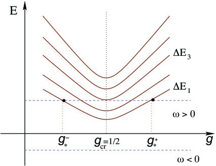
Figure 8: (Color Online) Sketch of the excitation spectrum of the Ising chain ${H}_{\rm{sys}}$ as a function of $g$. For a given frequency $\omega>0$, real saddle points correspond to intersections of the (solid) energy level curves (e.g., $\Delta E_{1}$) with the (dashed) vertical $\omega$-line which occur shortly before ($g_{*}^{-}$) and after ($g_{*}^{+}$) the quantum phase transition at $g_{\rm cr}=1/2$. The saddle-point approximation can only be applied if the intersection angle is large enough, i.e., for the drawn $\omega>0$ line, it would work for $\Delta E_{1}$, but not for $\Delta E_{3}$ etc.

$$\sum_{j}\left<\psi_{s}\right|\sigma_{x}^{j}(t)\left|\psi_{0}\right>\approx\frac{2ig(t)\sin(ka)}{\mathscr{E}_{k}(t)}\left<\psi_{s}\right|{\gamma}_{k}^{{\dagger}}{\gamma}_{-k}^{{\dagger}}\left|\psi_{0}\right>\,,$$

where the $\approx$ sign refers to the adiabatic approximation. Thus, it is only non-vanishing for excited states $\left|\psi_{s}\right>$ containing two quasi-particles $s=(k,-k)$ with opposite momenta and hence we get $\Delta E_{s0}=2\mathscr{E}_{k}$.

First of all, in order to have a quantum phase transition (or a working adiabatic quantum computer), the environment should be cold enough to permit the preparation of the system in the initial ground state such that $f(\omega)$ is only non-negligible when

$$\omega\ll 2=\mathscr{E}_{k}(t=0)$$ (40)

holds, compare also Eqn. (IV). Therefore, we will analyze the spectral excitation amplitude $\mathfrak{A}_{s}^{\omega}$ defined via

$$\mathfrak{A}_{s}\equiv\int d\omega\,f_{s}(\omega)\,\mathfrak{A}_{s}^{\omega}$$ (41)

in the different $\omega$-regimes in the following.

V.1.1 Intermediate Positive Frequencies

We may solve the time integral via the saddle-point (or stationary phase) approximation for intermediate positive frequencies,

$$2\gg\omega\gg\Delta E_{s0}^{\rm min}\approx 2|ka|\,.$$ (42)

For the exponent in Eqn. (37) the saddle-point condition reads

$$\left[\frac{\partial h_{k}(t,\omega)}{\partial t}\right]_{t=t_{*}}=0\,\,\leadsto\,\,\omega=\Delta E_{s0}(t_{*})=2\mathscr{E}_{k}(t_{*})\,,$$ (43)

where $h_{k}(t,\omega)=i\left[-\omega t+2\int_{0}^{t}dt^{\prime}\,\mathscr{E}_{k}(t^{\prime})\right]$ and $t_{*}$ denotes the saddle points. This condition yields two saddle points shortly before and after the transition, see also Fig. (8)

$$g(t_{*}^{\pm})=\frac{1}{2}\pm\frac{\left[\omega^{2}-16\sin^{2}\left(ka/2\right)\right]^{1/2}}{8\cos\left(ka/2\right)}\,.$$ (44)

The saddle-point approximation yields for the spectral excitation amplitude defined in (41)

$$\mathfrak{A}_{s}^{\omega\gg 2|ka|} \approx \sqrt{\frac{\pm 32\pi i\lambda^{2}\sin(ka)\sin\left(\frac{ka}{2}\right)e^{2h_{k}(t_{*},\omega)}}{\omega\dot{g}(t_{*})g^{-2}(t_{*})\sqrt{\omega^{2}-16\sin^{2}\left(\frac{ka}{2}\right)}}}$$ (45)

$$+{\cal O}\left(\frac{\lambda\dot{g}(t_{*})}{\omega\,\sqrt{\omega^{2}-4k^{2}a^{2}}}\right)\,,$$

which depends on the interpolation dynamics $g(t)$. The minimum gap can be obtained from Eqn. (34) and does indeed scale polynomially $\Delta E_{\rm min}={\cal O}(1/N)$ and, thus:

1. For a constant speed interpolation $g(t)=t/T$, the necessary run-time for an adiabatic evolution $T$ scales polynomially $T={\cal O}\left(\Delta E^{-2}_{\rm min}\right)={\cal O}(N^{2})$.

2. For adapted interpolation dynamics $\dot{g}(t)\propto\Delta E(t)$ or $\dot{g}(t)\propto\Delta E^{2}(t)$, however, one may achieve shorter run-times of $T={\cal O}(N\ln N)$ or $T={\cal O}(N)$, respectively schaller2006b and therefore better results for the spectral excitation amplitude, see Table 1.

V.1.2 Near the Minimum Gap

From Eqn. (45) it follows that the saddle-point approximation breaks down if $\omega$ approaches the minimum gap $w\approx\Delta E_{s0}^{\rm min}\approx 2|ka|$, see Fig. (8). In this case, we may obtain an upper bound for the time integral in Eqn. (37) via omitting all phases. For a constant speed interpolation $g(t)=t/T$

$$\mathfrak{A}_{s}^{\omega\approx 2|ka|} \leq \frac{2\lambda\sin(ka)}{T}\int_{0}^{T}dt\,\frac{t}{\mathscr{E}_{k}(t)}$$ (46)

$$= {\cal O}\left(\lambda N^{2}\omega\ln\omega\right)\,.$$

Similarly, one can get better results for adapted interpolation dynamics, see Table 1.

	$1\gg\omega\gg 2ka$	$1\gg\omega\approx 2ka$
$\ddot{g}(t)=0$	${\cal O}\left(\lambda ka\omega^{-1}N\right)$	${\cal O}\left(\lambda N^{2}\omega\ln\omega\right)$
$\dot{g}(t)\propto\Delta E(t)$	${\cal O}\left(\lambda ka\omega^{-3/2}\sqrt{N}\right)$	${\cal O}\left(\lambda N\ln N\right)$
$\dot{g}(t)\propto\Delta E^{2}(t)$	${\cal O}\left(\lambda ka\omega^{-2}\right)$	${\cal O}\left(\lambda N\right)$

Table 1: Scaling of the spectral excitation amplitude $\mathfrak{A}_{s}^{\omega}$ in the saddle-point approximation ($\omega\gg 2ka$) and its upper bound ($\omega\approx 2ka$) for different interpolation dynamics $g(t)$, where $\Delta E(t)=2\mathscr{E}_{k=\pi/(aN)}(t)$ denotes the fundamental gap. In all cases, the total excitation probability (integral over all $\omega$ and sum over all $k$) increases with system size $N$.

V.1.3 Positive Frequencies Below the Minimum Gap

For positive frequencies fulfilling $0\leq\omega\ll 2|ka|$, the saddle points at

$$g(t_{*}^{\pm})\approx\frac{1}{2}\,\pm\,\frac{1}{8}\sqrt{\omega^{2}-4k^{2}a^{2}}\,,$$ (47)

move away from the real axis and thus the exponent in Eqn. (37) contains real terms. The constant speed interpolation leads to

$$i\left[-\omega t_{*}+2\int_{0}^{t_{*}}dt\,\mathscr{E}_{k}(t)\right]\approx i\eta-\left[\frac{\omega|ka|}{4}+\frac{(ka)^{2}}{2}\right]T\,,$$

where $\eta$ is a real value. Therefore, the spectral excitation amplitude is exponentially suppressed in the adiabatic limit

$$\mathfrak{A}_{s}^{\omega\ll 2|ka|}={\cal O}\left(\exp\left\{-\frac{1}{2}\,T(ka)^{2}\right\}\right)\,.$$ (49)

V.1.4 Negative Frequencies

Finally, for negative frequencies $\omega<0$, the saddle points collide with the branch cut generated by the square-root in $\mathscr{E}_{k}$. In this case, we may also estimate the spectral excitation amplitude $\mathfrak{A}_{s}^{\omega}$ in Eqn. (41) by deforming the time integration contour into the complex plane. We assume that all involved functions can be analytically continued into the complex plane and are well-behaved near the real axis. Given this assumption, we deform the integration contour into the upper complex half-plane to obtain a negative exponent which is the usual procedure in such estimates until reaching a saddle point, a singularity, or a brunch cut, see Fig. (9). Deforming the integration contour into the lower complex half-plane would of course not change the result, but there the integrand is exponentially large and strongly oscillating such that the integral is hard to estimate. Since the integral in the complex plane is zero around path $c$ and the integrals on the paths 1 and 2 cancel each other, only paths $a$ and $b$ give the main contribution to the integral.

Let us first consider a constant interpolation function $g(t)=t/T$ which leads to singular points

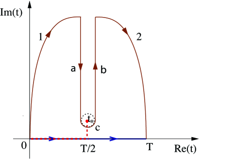
Figure 9: (Color Online) A sketch of the deformed integration contour. The original integration contour (blue line along the real axis) is shifted to the complex plane (curved line), where $t_{*}$ indicates the singular point, $t_{*}=T/2+iT/2\tan\left(ka/2\right)$. Only paths $a$ and $b$ contribute significantly to the integral.

$$t_{*}=\frac{T}{2}\pm i\frac{T}{2}\tan\left(\frac{ka}{2}\right)\,,$$ (50)

in the complex plane. Performing the time integral in the exponent of Eqn. (37) acquires a large negative real term in the exponent

$$\int_{0}^{t}dt^{\prime}\,\Delta E_{s0}(t^{\prime}) = \left\{\int_{0}^{T/2}+\int_{T/2}^{t_{*}}+\int_{t_{*}}^{t}\right\}dt^{\prime}\,\Delta E_{s0}(t^{\prime})$$ (51)

$$\approx \xi^{\prime}\pm 2t^{2}+\frac{i\pi T}{16}(ka)^{2}\,,$$

where $\xi^{\prime}$ is a constant and real value. Insertion of Eqn. (51) into Eqn. (37) and doing some algebra yields the exponential suppression for the amplitudes in the upper complex half-plane

$$\mathfrak{A}_{s}^{\omega<0} \approx \exp\left\{-\frac{\pi T}{16}\left(ka\right)^{2}\right\}\,\times$$ (52)

$$\times\,\int_{a,b}dt\,F(t)\exp\Big{\{}i\left(2t^{2}-\omega t+\tau\right)\Big{\}}$$

with $F(t)=\left<\psi_{s}(t)\right|\sum_{j}\sigma_{j}^{x}\left|\psi_{0}(t)\right>$ and where $\tau$ is a real constant. Therefore, applying the inequality

$$|\mathfrak{H}|\leq\int dy\,|\phi(y)|\quad{\rm with}\quad\mathfrak{H}=\int dy\,\phi(y)\,,$$ (53)

the amplitudes for negative frequencies are also exponentially suppressed for $g(t)=t/T$ and similarly for the other interpolations. This result can be understood in the following way: For frequencies $\omega$ below the lowest excitation energies, the energy $\omega$ of the reservoir modes is not sufficient for exciting the system via energy-conserving transitions. Hence excitations can only occur via non-adiabatic processes for which energy-conservation becomes ill-defined, but these processes are suppressed if the evolution is slow enough.

An estimate on the total error probability $|\mathfrak{A}_{s}|^{2}$ introduced in Eqn. (41) is obtained by performing the weighted sum of the contributions from the different $\omega$-regimes, which depends on the Fourier transform of the bath correlation function

$$\left|\mathfrak{A}_{s}^{\omega}\right| < \left[\max\limits_{\omega\gg 2|ka|}\left|\mathfrak{A}_{s}^{\omega\gg 2|ka|}\right|\right]\int\limits_{2\gg\omega\gg 2|ka|}\left|f_{s}(\omega)\right|d\omega$$ (54)

$$+\left[\max\limits_{\omega\approx 2|ka|}\left|\mathfrak{A}_{s}^{\omega\approx 2|ka|}\right|\right]\int\limits_{\omega\approx|ka|}\left|f_{s}(\omega)\right|d\omega$$

$$+\left[\max\limits_{0<\omega<2|ka|}\left|\mathfrak{A}_{s}^{\omega\ll 2|ka|}\right|\right]\int\limits_{0}^{2|ka|}\left|f_{s}(\omega)\right|d\omega$$

$$+\left[\max\limits_{\omega<0}\left|\mathfrak{A}_{s}^{\omega<0}\right|\right]\int\limits_{-\infty}^{0}\left|f_{s}(\omega)\right|d\omega\,.$$

From the results in Eqns. (45), (46), (49), and (52) it becomes obvious that although the last two contributions in the above sum can be efficiently suppressed, the first two terms will scale with the system size. Therefore, for the adiabatic Ising model, decoherence can only be effectively suppressed when the bath spectral function $f_{s}(\omega)$ has only support at frequencies below the minimum fundamental energy gap. For a bosonic bath in thermal equilibrium this would imply a reservoir temperature below the minimum fundamental energy gap, compare also Eqn. (IV).

V.2 Nonuniform Coupling Strengths

In a realistic situation, the Ising spins will not be symmetrically coupled to the environment

$$H_{\rm{int}}=\sum_{j}\sigma_{x}^{j}\otimes\delta B_{j}\,,$$ (55)

where $\delta B_{j}$ denote now different operators acting on the bath Hilbert space. Insertion of (55) into Eqn. (14) and evaluating the corresponding matrix element by applying the Jordan-Wigner, Fourier, and Bogoliubov transformations of Pauli matrices – given in Eqns. (V), (29), and (30) – yield

$$\mathfrak{A}_{s} \approx -\frac{2i\lambda}{N}\sum_{k,k^{\prime}}\int d\omega\,f_{k,k^{\prime}}^{s}(\omega)\int_{0}^{T}dt\,\,u_{k}^{*}(t)\,v_{k^{\prime}}(t)\times$$

$$\left<\psi_{s}(t)\right|\gamma_{k}^{\dagger}\,\gamma_{-k^{\prime}}^{\dagger}\left|\psi_{0}(t)\right>\,\exp\left\{i\left[-\omega t+\int_{0}^{t}dt^{\prime}\,\Delta E_{s0}(t^{\prime})\right]\right\}\,,$$

where we include again all relevant properties of the environment into the spectral function $f_{k,k^{\prime}}^{s}(\omega)$ of the bath

$$e^{-i\Delta\varphi^{\prime}_{s}(t)}\left(\sum_{j}\delta B^{s0}_{j}\,e^{i(k-k^{\prime})ja}\right)\equiv\int_{-\infty}^{+\infty}d\omega\,e^{-i\omega t}f_{k,k^{\prime}}^{s}(\omega)\,,$$

where $\delta B^{sr}_{j}=\left<\alpha_{s}(t)\right|\delta B_{j}(t)\left|\alpha_{r}(t)\right>$, $\Delta\varphi^{\prime}_{s}$ coincides with $\varphi_{s}-\varphi_{0}$ in Eqn. (III) apart from the system’s energy gap $\Delta E_{s0}$ and $u_{k}(t)$, $v_{k}(t)$ are the Bogoliubov coefficients given in Eqn. (V). The excitation amplitude in Eqn. (V.2) is only non-vanishing for the excited states containing two quasi-particles $s=(k,-k^{\prime})$

$$\Delta E_{s0}=\mathscr{E}_{k}+\mathscr{E}_{k^{\prime}}\,.$$ (58)

Insertion of $\displaystyle{u_{k}^{*}}$, $\displaystyle{v_{k^{\prime}}}$ given by Eqn. (V), into Eqn. (V.2) yields

$$\mathfrak{A}_{s} \approx \frac{i\lambda}{N}\sum_{k,k^{\prime}}\int d\omega\,f_{k,k^{\prime}}^{s}(\omega)\int_{0}^{T}dt\left<\psi_{s}(t)\right|\gamma_{k}^{\dagger}\,\gamma_{-k^{\prime}}^{\dagger}\left|\psi_{0}(t)\right>\times$$ (59)

$$\times\,\frac{{\cal C}_{k,k^{\prime}}(t)}{{\cal N}_{k^{\prime}}}\,\exp\left\{i\left[-\omega t+2\int_{0}^{t}dt^{\prime}\,\mathscr{E}_{k}(t^{\prime})\right]\right\}\,,$$

where

$${\cal C}_{k,k^{\prime}}(t)=4\,g(t)\,\sin(k^{\prime}a)\sqrt{\frac{1}{2}+\frac{1-2g(t)\cos^{2}(ka/2)}{\mathscr{E}_{k}(t)}}\,.$$

Following the same procedure outlined above, we may consider different domains of $\omega$ in order to solve the time integral in Eqn. (59). For the intermediate positive frequencies,

$$2\gg\omega\gg 2\,|ka|\,\,\,{\rm{and}}\,\,\,2\,|k^{\prime}a|\,,$$ (61)

the saddle-point approximation can be applied once again

$$-\omega+\,2\,\mathscr{E}_{k}(t_{*})=0\,,$$ (62)

where $t_{*}$ denotes the saddle points. The saddle-point approximation yields for the spectral excitation amplitude

$$\mathfrak{B}_{s}^{\omega\gg 2|ka|}={\cal O}\left(\frac{\lambda k^{\prime}a}{N\sqrt{\omega\,\dot{g}(t_{*})\sqrt{\omega^{2}-4{k}^{2}a^{2}}}}\right)\,,$$ (63)

where $\displaystyle{\mathfrak{B}_{s}^{\omega}}$ is defined as following

$$\mathfrak{A}_{s}\approx\sum_{k,k^{\prime}}\int d\omega\,f_{k,k^{\prime}}^{s}(\omega)\,\mathfrak{B}_{s}^{\omega}\,.$$ (64)

The spectral excitation amplitude in Eqn. (63) depends on the interpolation dynamics $g(t)$ and is very similar to Eqn. (45) apart from $N$ in the denominator. Presence of $N$ in the denominator may cause some slow down for the error probability, see Table 1. However, existence of many excited states – sum over all possible $k$ and $k^{\prime}$ in Eqn. (59) – causes the growth of the error probability with the system size. If $\omega$ approaches the $2|ka|$, the saddle-point approximation breaks down and we can get a similar upper bound which is shown in Table. 1, by omitting all phases. With the same argument given above, the amplitudes are exponentially suppressed in the adiabatic limit for frequencies far below $2|ka|$. Thus, as with the discussion in the previous subsection below Eqn. (54) we may conclude that in a more general case where the coupling strength to the bath is not uniform, the impact of decoherence for the environmental noise is very similar to the coherent reservoir and the error probability increases with the system size, unless the bath temperature lies below the minimum energy gap.

V.3 Perturbing the Bitflip Symmetry

Unfortunately, interactions with the reservoir cannot be tailored, such that one may also expect perturbations that do not reflect the bitflip symmetry of the Ising Hamiltonian and thereby lead to leakage between the subspaces of even and odd quasi-particle numbers. Let us consider a simple case, where only one Ising spin is coupled to the environment

$$H_{\rm{int}}=\sigma_{z}^{1}\otimes\delta B\,.$$ (65)

Insertion of this interaction Hamiltonian into Eqn. (14) and evaluating the corresponding matrix element yield the excitation amplitude which is a combination of two terms

$$\mathfrak{A}_{s}=\,-\,\frac{i\,\lambda}{\sqrt{N}}\,\int d\omega\,f_{s}(\omega)\sum_{k}\left(\mathfrak{A}^{\omega}_{s,1}+\mathfrak{A}^{\omega}_{s,2}\right)\,,$$ (66)

with

$$\mathfrak{A}^{\omega}_{s,1} \approx i\,e^{-ika}\,\int_{0}^{T}dt\,\frac{\beta_{k}}{{\cal N}_{k}}\,\left<\psi_{s}(t)\right|\gamma_{-k}^{\dagger}\left|\psi_{0}(t)\right>\,e^{-i\omega t}$$

and

$$\mathfrak{A}^{\omega}_{s,2} \approx e^{ika}\,\int_{0}^{T}dt\,\sqrt{\frac{1}{2}+\frac{1-2g(t)\cos^{2}(ka/2)}{\mathscr{E}_{k}(t)}}\times$$

$$\times\,\left<\psi_{s}(t)\right|\gamma_{k}^{\dagger}\left|\psi_{0}(t)\right>\exp\left\{i\left[-\omega t+2\int_{0}^{t}dt^{\prime}\,\mathscr{E}_{k}(t^{\prime})\right]\right\}\,,$$

where the spectral function $f_{s}(\omega)$ of the bath is as defined in Eqn. (V.1). For large $T$, the first term $\mathfrak{A}^{\omega}_{s,1}$ is a Fourier transformation of some function of $\omega$

$$\mathfrak{A}^{\omega}_{s,1}\approx ie^{-ika}\sin(ka)\underbrace{\left(\Sigma(\omega)-\underbrace{\int_{-T}^{0}dt\,\,\Xi(t)\,e^{-i\omega t}}_{{\cal O}\left(1/\omega\right)}\right)}_{\Omega(\omega)}\,,$$

where

$$\Xi(t)=\frac{2g(t)}{\sqrt{2\mathscr{E}^{2}_{k}(t)+4\left[1-2g(t)\cos^{2}(ka/2)\right]\mathscr{E}_{k}(t)}},$$ (70)

$\Sigma(\omega)=\int_{-T}^{T}dt\,\Xi(t)\,e^{-i\omega t}$, and $\Omega(\omega)$ is some function of $\omega$. In order to solve the time integral of $\mathfrak{A}^{\omega}_{s,2}$, we may employ saddle point approximation which yields

$$\mathfrak{A}^{\omega}_{s,2}={\cal O}(T)\,.$$ (71)

Thus, we can conclude that

$$\mathfrak{A}_{s}=\int d\omega\,f_{s}(\omega)\sum_{k}\underbrace{\left[{\cal O}\left(\frac{\lambda ka}{\sqrt{N}}\right)+{\cal O}\left(\frac{\lambda T}{\sqrt{N}}\right)\right]}_{\mathfrak{A}^{\omega}_{s}}\,.$$ (72)

The optimal run-time for an adiabatic evolution $T$ depends on the interpolation dynamics $g(t)$, see schaller2006b . Scaling of the spectral excitation amplitude $\mathfrak{A}^{\omega}_{s}$ for different interpolation dynamics is shown in Table 2.

	$\mathfrak{A}^{\omega}_{s}$
$\ddot{g}(t)=0$	${\cal O}\left(\lambda ka/\sqrt{N}\right)+{\cal O}\left(\lambda N^{3/2}\right)$
$\dot{g}(t)\propto\Delta E(t)$	${\cal O}\left(\lambda ka/\sqrt{N}\right)+{\cal O}\left(\lambda\sqrt{N}\ln N\right)$
$\dot{g}(t)\propto\Delta E^{2}(t)$	${\cal O}\left(\lambda ka/\sqrt{N}\right)+{\cal O}\left(\lambda\sqrt{N}\right)$

Table 2: Scaling of the spectral excitation amplitude $\mathfrak{A}_{s}^{\omega}$ for different interpolation dynamics $g(t)$, where $\Delta E(t)=\mathscr{E}_{k=\pi/(aN)}(t)$ denotes the fundamental gap. In all cases, the total excitation probability (integral over all $\omega$ and sum over all $k$) increases with system size $N$.

This decoherence channel poses a significant problem to robust ground state preparation in the Ising model: Regardless how low the bath temperature is, the decoherent excitation probability will scale with the system size! This finding is consistent with the experience that large Schrödinger cat states as (6) are extremely sensitive to decoherence.

VI Summary

In summary, we studied the impact of decoherence due to a weak coupling to a rather general environment on first and second order quantum phase transitions. Since the Ising model is considered sachdev as a prototypical example for a second-order quantum phase transition, we expect our results to reflect general features of second-order transitions.

For the decoherence channel (36) which is always present (though possibly not the dominant channel), we already found that the total excitation probability always increases with system size $N$ (continuum limit): Even though the probability for the lowest excitation $k=\pm\pi/(aN)$ can be kept under control for a bath which is well-behaved in the infra-red limit – see also Sec. (3.4) – the existence of many excited states $k\in\pi(1+2{\mathbb{Z}})/(aN)\;:\;|ka|<\pi$ converging near the critical point causes the growth of the error probability for large systems. This growth can be slowed down a bit via adapted interpolation schemes $g(t)$, but not stopped.

Other decoherence channels will in the best case display the same general behavior: E.g., for $2\gg\omega\gg|ka|$, the associated amplitudes scale as

$$\mathfrak{A}_{s}^{\omega}={\cal O}\left(\frac{\lambda\phi_{s}(t_{*})}{\sqrt{\dot{g}(t_{*})}}\right)\,,$$ (73)

where $\phi_{s}$ denotes the matrix element in analogy to (V.1). Typically, for a homogeneous coupling to the bath, $\phi_{s}$ does not strongly depend on the system size $N$ (for given $ka$ and $\omega$). Since $\dot{g}(t_{*})$ decreases for $N\to\infty$ or at least remains constant – for $\dot{g}(t)\propto\Delta E^{2}(t)$ – the total excitation probability again increases with system size $N$. If only a few spins are coupled via $\sigma^{x}_{j}$ to the environment, the matrix element $\phi_{s}$ in Eqn. (V.2) will decrease with the system size ${\cal O}(1/N)$ and then the error probability may be kept under control – for $\dot{g}(t)\propto\Delta E^{2}(t)$. However, $\phi_{s}$ is of order ${\cal O}(1/\sqrt{N})$ for the the $\sigma^{z}$-channel given in Eqn. (66) and the Schrödinger cat states are still sensitive to decoherence.

According to the analogy between adiabatic quantum algorithms and quantum phase transitions latorre ; gernot , this result suggests scalability problems of the corresponding adiabatic quantum algorithm – unless the temperature of the bath stays below the ($N$-dependent) minimum gap childs_robust or the coupling to the bath decreases with increasing $N$. These problems are caused by the accumulation of many levels at the critical point $g_{\rm cr}=1/2$, which presents the main difference to isolated avoided level crossings (corresponding to first-order phase transitions) discussed earlier. It also causes some difficulties for the idea of thermally assisted quantum computation (see, e.g., amin ) since, in the presence of too many available levels, the probability of hitting the ground state becomes small.

Therefore, in order to construct a scalable adiabatic quantum algorithm in analogy to the Ising model, suitable error-correction methods will be required. As one possibility, one might exploit the quantum Zeno effect and suppress transitions in the system by constantly measuring the energy, see for example childs_zeno . Another interesting idea are adiabatic ground state preparation schemes (algorithms) that provide a constant lower bound on the fundamental energy gap that does not scale with the system size. In case of the Ising model discussed here, this is possible by increasing the complexity of the interpolation path (i.e., beyond the straight-line interpolation). Unfortunately, the simplest approach to the Ising model gernot-nonlinear only bounds the fundamental gap in the subspace of even bitflip parity, i.e., decoherence channels that mediate transitions between the two subspaces as e.g. in Eqn.  (65) will destroy the associated robustness against decoherence. Many-body interactions in the system Hamiltonian are required to resolve this problem. In this case, decoherence could be strongly suppressed for a low-temperature bath. Of course, the generalization of all these concepts and results to more interesting cases such as the (NP-complete) two-dimensional Ising model is highly non-trivial and requires further investigations.

VII Acknowledgments

This work was supported by the DFG (SCHU 1557/1-2,3; SCHU 1557/2-1; SFB-TR12).

^∗ ralf.schuetzhold@uni-due.de

References

- (1) S. Sachdev, Quantum phase transitions, (Cambridge University Press, Cambridge, UK, 1999).
- (2) M. A. Nielsen and I. L. Chuang, Quantum computation and quantum information, (Cambridge University Press, Cambridge, England, 2000).
- (3) E. Farhi, J. Goldstone, S. Gutmann and M. Sipser, pre-print: quant-ph/0001106 (2000).
- (4) A. M. Childs, E. Farhi, and J. Preskill, Phys. Rev. A 65, 012322 (2001).
- (5) M. S. Sarandy, and D. A. Lidar, Phys. Rev. Lett. 95, 250503 (2005).
- (6) A. Messiah, Quantum mechanics, (John wiley and Sons, 1958).
- (7) J. I. Latorre and R. Orús, Phys. Rev. A 69, 062302 (2004).
- (8) R. Schützhold and G. Schaller, Phys. Rev. A 74, 060304(R) (2006).
- (9) J. Roland and N. J. Cerf, Phys. Rev. A 65, 042308 (2002).
- (10) J. E. Bunder and R. H. McKenzie, Phys. Rev. B 60, 344 (1999).
- (11) K. H. Fischer, and J. A. Hertz, Spin glasses, (Cambridge University Press, Cambridge, UK, 1993).
- (12) A. Das, and B. K. Chakrabarti, (LNP 679, Springer-Verlag, Heidelberg, 2005).
- (13) G. E. Santoro, R. Martoňák, E. Tosatti, and R, Car, Science 295, 2427 (2002).
- (14) T. Kadowaki, and H. Nishimori, Phys. Rev. E 58, 5355 (1998).
- (15) http://tinyurl.com/yoz77v, see also W. van Dam, Nature Physics 3, 220 (2007).
- (16) S. Mostame, G. Schaller, and R. Schützhold, Phys. Rev. A 76, 030304(R) (2007).
- (17) J. Dziarmaga, Phys. Rev. Lett. 95, 245701 (2005).
- (18) G. Schaller, and R. Schützhold, Quantum Information and Computation 10, 0109 (2010).
- (19) R. Schützhold, Journal of Low Temperature Physics 153, 228-243 (2008).
- (20) G. Schaller and T. Brandes, Phys. Rev. A 78, 022106 (2008).
- (21) T. Brandes, Physics Reports 408, 315-474 (2005).
- (22) E. Farhi, J. Goldstone, Sam Gutmann and Daniel Nagaj, International Journal of Quantum Information 6, 503 (2008).
- (23) M. Z̆nidaric̆, and M. Horvat, Phys. Rev. A 73, 022329 (2006).
- (24) R. Schützhold, M. Uhlmann, Y. Xu and Uwe R. Fischer, Phys. Rev. Lett. 97, 200601 (2006).
- (25) R. Schützhold, Phys. Rev. Lett. 95, 135703 (2005).
- (26) G. Vidal, J. I. Latorre, E. Rico, and A. Kitaev, Phys. Rev. Lett. 90, 227902 (2003).
- (27) W. H. Zurek, U. Dorner, and P. Zoller, Phys. Rev. Lett. 95, 105701 (2005).
- (28) B. Damski, Phys. Rev. Lett. 95, 035701 (2005).
- (29) K. Sengupta, S. Powell, and S. Sachdev, Phys. Rev. A 69, 053616 (2004).
- (30) D. Patane, L. Amico, A. Silva, R. Fazio, and G. E. Santoro, Phys. Rev. B 80, 024302 (2009).
- (31) A. Fubini, G. Falci and A. Osterloh, New J. Phys. 9, 134 (2007).
- (32) M. S. Sarandy, L. A. Wu, and D. A. Lidar, Quant. Inf. Proc. 3, 331 (2004).
- (33) M. Tiersch and R. Schützhold, Phys. Rev. A 75, 062313 (2007).
- (34) G. Schaller, S. Mostame, and R. Schützhold, Phys. Rev. A 73, 062307 (2006).
- (35) S. Jansen, M. B. Ruskai, and R. Seiler, J. Math. Phys. 48, 102111 (2007).
- (36) P. Jordan and E. Wigner, Z. Phys. 47, 631 (1928).
- (37) S. Katsura, Phys. Rev. 127, 1508 (1962).
- (38) M. H. S. Amin, Peter J. Love, and C. J. S. Truncik, Phys. Rev. Lett. 100, 060503 (2008).
- (39) A. M. Childs, E. Deotto, E. Farhi, J. Goldstone, S. Gutmann and A. J. Landahl, Phys. Rev. A 66, 032314 (2002).
- (40) G. Schaller, Phys. Rev. A 78, 032328 (2008)