Extraction of Transition Form Factors for Nucleon Resonances within a Coupled-Channels Model

Abstract

We explain how an analytic continuation we have developed recently is applied to determine the residues of the nucleon resonance poles within a dynamical coupled-channel model of meson-baron reactions. A procedure for evaluating the electromagnetic $N$-$N^{*}$ transition form factors at resonance poles is developed. Illustrative results of the obtained $N^{*}\rightarrow\pi N,\gamma N$ transition form factors for $P_{11}$, $P_{33}$, and $D_{13}$ nucleon resonances are presented and compared with previous results.

I Introduction

In a recent paperssl09 , we have developed an analytic continuation method to determine nucleon resonances within a dynamical coupled-channel model of meson-baryon reactionsmsl07 (MSL). The method has been appliedsjklms09 to extract 14 nucleon resonances from the $\pi N$ model developed in Ref.jlms07 (JLMS) which has been extended to investigate $\pi N,\gamma N\rightarrow\pi\pi N$kjlms09 , $\gamma N\rightarrow\pi N$jlmss08 and $N(e,e^{\prime}\pi)N$jklmss09 reactions. The purpose of this paper is to explain how the residues of the extracted resonance poles are determined from the predicted $\pi N\rightarrow\pi N$ and $\gamma^{*}N\rightarrow\pi N$ amplitudes.

In section II, we briefly review the analytic continuation method developed in Ref.ssl09 . Section III is devoted to explaining the determination of the residues of the nucleon resonance poles. Illustrative results for $P_{11}$, $P_{33}$, and $D_{13}$ nucleon resonances are presented in section IV and compared with the results from other analysis. A summary is given in section V.

II Analytic continuation method

Within the MSL formulationmsl07 , the partial wave amplitudes of two-body meson-baryon reactions can be written as

$$T_{\beta,\alpha}(p^{\prime},p;E) = t_{\beta,\alpha}(p^{\prime},p;E)+t^{R}_{\beta,\alpha}(p^{\prime},p;E)\,,$$ (1)

where $\alpha,\beta$ represent the meson-baryon (MB) states $\gamma N$, $\pi N,\eta N,\rho N,\sigma N,\pi\Delta$, and

$$t^{R}_{\beta,\alpha}(p^{\prime},p;E) = \sum_{i,j}\bar{\Gamma}_{\beta,i}(p^{\prime};E)[G_{N^{*}}(E)]_{i,j}\bar{\Gamma}_{\alpha,j}(p;E)$$ (2)

with

$$[G_{N^{*}}^{-1}]_{i,j}(E) = (E-m_{N^{*}_{i}})\delta_{i,j}-\Sigma_{i,j}(E)\,.$$ (3)

Here $i,j$ denote the bare $N^{*}$ states defined in the Hamiltonian. $m_{N^{*}_{i}}$ are their masses. The first term (called meson-exchange amplitude from nowon) in Eq.(1) are defined by the following equation

$$t_{\beta,\alpha}(p^{\prime},p;E) = v_{\beta,\alpha}(p^{\prime},p)+\int_{C}dqq^{2}\sum_{\gamma}v_{\beta,\gamma}(p^{\prime},q;E)G_{\gamma}(q,E)t_{\gamma,\alpha}(q,p;E)$$ (4)

where $v_{\beta,\alpha}$ is defined by the meson-exchange mechanisms, and $G_{\gamma}(q,E)$ is the propagator for channel $\gamma$. The dressed vertices and the energy shifts of the second term in Eqs.(2)-(3) are defined by

$$\bar{\Gamma}_{\alpha,j}(p;E) = \Gamma_{\alpha,j}(p)+\int_{C}dqq^{2}\sum_{\gamma}t_{\alpha,\gamma}(p^{\prime},q;E)G_{\gamma}(q,E)\Gamma_{\gamma,j}(q)$$ (5)

$$\Sigma(E)_{i,j} = \int_{C}dqq^{2}\sum_{\gamma}\Gamma_{\gamma,i}(q)G_{\gamma}(q,E)\bar{\Gamma}_{\gamma,j}(q).$$ (6)

where $\Gamma_{\alpha,i}(p)$ defines the coupling of the $i$-th bare $N^{*}$ state to channel $\alpha$.

To search for nucleon resonances, we have developedssl09 an analytic continuation method to find poles of the scattering amplitude $T_{\alpha,\beta}(p^{\prime},p;E)$ on the unphysical sheets of the complex energy $E$-plane. For multi-channel reactions considered here, there can be many poles associated with a single resonance on different unphysical sheets. The pole nearest to the physical sheet is supposed to play a dominant effect on physical observables, and is called the resonance pole traditionally. The other poles are called shadow poles.

Since $v_{\alpha,\beta}$ and the bare vertex $\Gamma_{\alpha,i}$ are energy independent within the MSL formulation, the analytic structure of the scattering amplitude defined above as a function of $E$ is mainly determined by the the Green functions $G_{\gamma}(q,E)$. Thus the key for selecting the amplitude on physical sheet or unphysical sheet is to take an appropriate path of momentum integration $C$ in Eqs.(1)-(6) according to the locations of the singularities of the meson-baryon Green functions $G_{\alpha}(p,E)$ as $E$ move to complex plane. This can be done independently for each meson-baryon channel. For channel with stable particles such as $\pi N$ and $\eta N$, the meson-baryon Green function is

$$G_{MB}(E,p)=\frac{1}{E-E_{M}(p)-E_{B}(p)}\,,$$ (7)

which has a pole at the on-shell momentum $p_{0}$ defined by

$$E=\sqrt{m_{M}^{2}+p^{2}_{0}}+\sqrt{m_{B}^{2}+p^{2}_{0}}.$$ (8)

As an example, let us consider the analytic continuation of the amplitude to the unphysical sheet of the $MB$ channel when the energy $E$ is above the threshold $Re(E)>m_{B}+m_{M}$ and $Im(E)<0$. The on-shell momentum $p_{0}$ for such a $E$ is on the second and the fourth quadrant of the complex momentum plane. As $Im(E)$ becomes more negative as illustrated in Fig. 1, the on-shell momentum (open circle) moves into the fourth quadrant. The amplitude on the unphysical sheet can be obtained by deforming the path $C$ into $C_{1}^{\prime}$ or equivalently $C_{1}$ so that the on-shell momentum does not cross the integration contour. We note here that for the energy below threshold ($Re(E)<m_{B}+m_{M}$) the path $C_{1}$ will give amplitudes on the physical sheet.

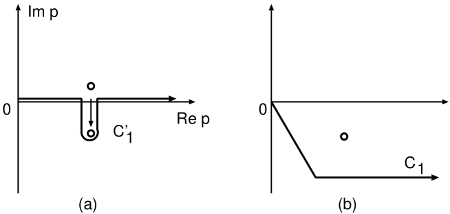
Figure 1: The shift of the on-shell momentum (open circle) of the two-particle Green function Eq. (7) as energy E moves from a real value above the threshold energy to a complex value with negative imaginary part. $C^{\prime}_{1}$ in (a) or $C_{1}$ in (b) is the integration path for calculating Eqs.(4)-(6) amplitude for E on the unphysical plane.

For the channels with unstable particle such as the $\pi\Delta$ as an example, the Green function is of the following form

$$G_{\pi\Delta}(E,p)=\frac{1}{E-E_{\pi}(p)-E_{\Delta}(p)-\Sigma_{\Delta}(E,p)},$$ (9)

where

$$\Sigma_{\Delta}(p,E)=\int_{C_{3}}\frac{\{\Gamma_{\Delta,\pi N}(q)\}^{2}q^{2}dq}{E-E_{\pi}(p)-[(E_{\pi}(q)+E_{N}(q))^{2}+p^{2}]^{1/2}}.$$

(10)

The $\pi\Delta$ Green function Eq. (9) has a singularity at momentum $p=p_{x}$, which satisfies

$$E-E_{\pi}(p_{x})-E_{\Delta}(p_{x})-\Sigma_{\Delta}(p_{x},E)=0.$$ (11)

Physically, this singularity corresponds to the $\pi\Delta$ two-body ’scattering state’. There is also discontinuity of the $\pi\Delta$ Green function associated with the $\pi\pi N$ cut in $\Sigma_{\Delta}$, as shown in the dashed line in Fig. 2, where $p_{0}$ is defined by

$$E=E_{\pi}(p_{0})+[(m_{\pi}+m_{N})^{2}+p^{2}_{0}]^{1/2}.$$ (12)

Therefore, for $Re(E)>m_{B}+m_{M},2m_{\pi}+m_{N}$, the integration contour $C$ must be chosen to be below the $\pi\pi N$ cut (dashed line) and the singularity $p_{x}$, such as the contour $C_{2}$ shown in Fig.2, for calculating amplitudes on the unphysical sheet.

The singularity $q_{0}$ of the integrand of Eq. (10) depends on the spectator momentum $p$

$$E-E_{\pi}(p)=[(E_{\pi}(q_{0})+E_{N}(q_{0}))^{2}+p^{2}]^{1/2}\,.$$ (13)

Thus $q_{0}$ moves along the dashed curve, illustrated in Fig.3, when the momentum $p$ varies along the path $C_{2}$ of Fig.2. To analytically continue $\Sigma_{\Delta}(p,E)$ to the unphysical sheet, the contour $C_{3}$ of Eq. (10) must be below $q_{0}$. A possible contour $C_{3}$ is the solid curve in Fig.3.

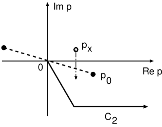
Figure 2: Contour $C_{2}$ for for calculating Eqs.(4)-(6) for E on the unphysical plane with the unstable particle propagators, such as Eq.(9) for $\pi\Delta$ channel. See the text for the explanations of the dashed line and the singularity $p_{x}$.

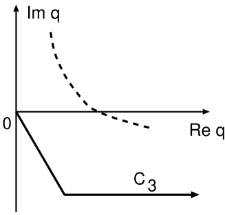
Figure 3: Contour $C_{3}$ for calculating the $\Delta$ self energy Eq.(10) on the unphysical sheet. Dashed curve is the singularity $q_{0}$ of the propagator in Eq. (13), which depends on the spectator momentum $p$ on the contour $C_{2}$ of Fig.2.

We emphasize here that we can deform the contour $C$ only in the region where the potential $v_{\alpha,\beta}(p^{\prime},p)$ and the bare $N^{*}$ vertex $\Gamma_{MB,N^{*}}(p)$ are analytic. The contours described above only from considering the singularities of $MB$ and $\pi\pi N$ Green functions. Thus they must be modified according to the analytic structure of the considered $v_{\alpha,\beta}(p^{\prime},p)$ and $\Gamma_{MB,N^{*}}(p)$. Within the MSL formulation, the t-channel meson exchange potential $v^{t}_{M^{\prime}B^{\prime},MB}(\vec{p}^{\,\,{}^{\prime}},\vec{p})$ has singularities at

$$\Delta^{2}-(\vec{p}-\vec{p}^{\prime})^{2}=0$$ (14)

with $\Delta=E_{M^{\prime}}(p^{\prime})-E_{M}(p)$ or $E_{B^{\prime}}(p^{\prime})-E_{B}(p)$. The form of $\Gamma_{MB,N^{*}}(p)$ is chosen such that its singularity is at the pure imaginary momentum. Thus the contours have to be chosen to also avoid these singularities. As an example we show in Fig.4 the singularities associated with the $\pi\Delta$ channel at $E=1357-76i$MeV. The dotted line for $\pi\pi N$ cut and the circle shows $p_{X}$ are the singularities from the Green’s function, as discussed above. The most relevant singularity of the meson-exchange potential in our investigation of electromagnetic pion production amplitude is due to the t-channel pion exchange of $\gamma N\rightarrow\pi\Delta$, which is shown as the dashed-dot curve. Thus the integration contour has to be modified to the solid curve in Fig.4.

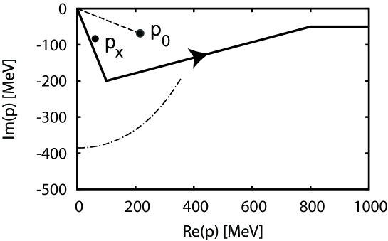
Figure 4: The contour (solid curve) for calculating electromagnetic matrix element. $p_{0}$ and $p_{x}$ are the singularities shown in Fig.2. The dashed-dot curve is the singularity of the pion-exchange $\gamma N\rightarrow\pi N$ matrix element at $E=1357-76i$ MeV.

III Extraction of resonance parameters

The resonance energy ($M_{R}=M-i\Gamma/2$) is the position of the pole of the scattering amplitude which is on the sheet nearest to the physical sheet. In principle the resonance pole can be found in the meson-exchange amplitude $t$ and/or resonance amplitude $t^{R}$ of Eq. (1). Within the $\pi N$ model developed in Ref.jlms07 (JLMS), we findsjklms09 that resonance poles are only from $t^{R}$. We therefore will only explain how the residues of resonance poles are extracted from this term.

The poles of $t^{R}$ are found from the zeros of the determinant of $N^{*}$ propagator defined by Eq.(3)

$$\Delta(E)=det[G_{N^{*}}^{-1}(E)] = 0\,.$$ (15)

Near the resonance energy $M_{R}$, $N^{*}$ Green function can be expressed as

$$(G_{N^{*}}(E))_{ij} = \frac{\chi_{i}\chi_{j}}{E-M_{R}}\,,$$ (16)

where $i,j$ denote the bare $N^{*}$ state in the Hamiltonian and $\chi_{i}$ represents $i$-th component of the dressed $N^{*}$ and satisfies

$$\sum_{j}(G_{N^{*}}(M_{R})^{-1})_{ij}\chi_{j} = \sum_{j}[(M_{R}-m_{N^{*}_{i}})\delta_{ij}-\Sigma(M_{R})_{ij}]\chi_{j}=0.$$ (17)

If there is only one bare $N^{*}$ state, it is easy to see that

$$\chi = \frac{1}{\sqrt{1-\Sigma^{\prime}(M_{R})}}\,,$$ (18)

where $\Sigma^{\prime}(M_{R})=[d\Sigma/dE]_{E=M_{R}}$. If we have two bare $N^{*}$ states, we find that

$$\chi_{1} = \sqrt{\frac{M_{R}-m_{N^{*}_{2}}-\Sigma_{22}(M_{R})}{\Delta^{\prime}(M_{R})}}\,,$$ (19)

$$\chi_{2} = \frac{\Sigma_{12}(M_{R})}{M_{R}-m_{N^{*}_{2}}\,,-\Sigma_{22}(M_{R})}\chi_{1}$$ (20)

where $\Delta^{\prime}(M_{R})=[d\Delta/dE]_{E=M_{R}}$ can be evaluated using Eq.(15).

We now examine how the residues $\chi_{i}$ can be used to see the effects of resonance poles on the full amplitude $T_{\alpha,\beta}$ defined by Eq.(1). Near the resonance pole we can perform Laurent expansion of the on-shell amplitude

$$T_{\alpha,\beta}(p^{0}_{\alpha},p^{0}_{\beta},M_{R})=\frac{\bar{\Gamma}^{R}_{\alpha}\bar{\Gamma}^{R}_{\beta}}{E-M_{R}}+C^{0}_{\alpha,\beta}+C^{1}_{\alpha,\beta}(E-M_{R})+...\,.$$ (21)

For the cases that the resonance poles are from $t^{R}$ term of Eq.(1), one can see from the definitions Eqs.(2)-(3) and Eq.(16) that the vertex functions in the residue of Eq.(21) is determined by the dressed vertex $\bar{\Gamma}_{\alpha,j}$ defined by Eq.(5)

$$\bar{\Gamma}^{R}_{\alpha} = \sum_{j}\chi_{j}\bar{\Gamma}_{\alpha,j}(p^{0}_{\alpha},M_{R}).$$ (22)

The terms $C^{0}_{\alpha,\beta}$ and $C^{1}_{\alpha,\beta}$ in Eq.(21) also depend on the matrix elements of meson-exchange amplitude $t$ of Eq.(1), but will not be discussed here.

The residue of the $\pi N$ elastic scattering amplitude $F_{\pi N,\pi N}$ characterizes the strength of the coupling of the resonance with $\pi N$ channel. Using the standard notation, we have at near resonance position $M_{R}$

$$F_{\pi N,\pi N}(E) = \frac{S_{\pi N,\pi N}(E)-1}{2i}=[\frac{Re^{i\phi}}{M_{R}-E}]_{E\rightarrow M_{R}}\,,$$ (23)

where $S_{\pi N,\pi N}$ is the partial-wave S-matrix. In terms of the normalization of JLMS model, we have

$$F_{\pi N,\pi N}(M_{R})=-\pi\frac{p_{0}E_{N}(p_{0})E_{\pi}(p_{0})}{M_{R}}T_{\pi N,\pi N}(p_{0},p_{0},M_{R})$$ (24)

We thus have

$$Re^{i\phi} = \pi\frac{p_{0}E_{N}(p_{0})E_{\pi}(p_{0})}{M_{R}}\bar{\Gamma}^{R}_{\pi N}\bar{\Gamma}^{R}_{\pi N}\,.$$ (25)

The elasticity of a resonance is then defined as

$$\eta_{e}=\frac{R}{-Im(M_{R})}$$ (26)

The electromagnetic $N$-$N^{*}$ transition form factor is defined by matrix element of the electromagnetic currents between nucleon and $N^{*}$

$$A_{3/2}(Q^{2}) = X<N^{*},s_{z}=3/2|-\vec{J}(Q^{2})\cdot\vec{\epsilon}_{+1}|N,s_{N}=1/2>\,,$$ (27)

$$A_{1/2}(Q^{2}) = X<N^{*},s_{z}=1/2|-\vec{J}(Q^{2})\cdot\vec{\epsilon}_{+1}|N,s_{N}=-1/2>\ ,,$$ (28)

$$S_{1/2}(Q^{2}) = X<N^{*},s_{z}=1/2|J^{0}(Q^{2})|N,s_{N}=1/2>\,,$$ (29)

where $\vec{\epsilon}_{+1}=-(\hat{x}+i\hat{y})/\sqrt{2}$,

$$X = \sqrt{\frac{E_{N}(\vec{q})}{m_{N}}}\frac{1}{\sqrt{2K}}\,,$$

with $K=(M_{R}^{2}-m_{N}^{2})/(2M_{R})$. The above definition was originally introduced for the constituent quark modelcopley . If $<N^{*}|$ is a resonance state, then the above expression at resonance position $M_{R}$ must be evaluated by using Eq.(22). We thus have

$$A_{3/2}(Q^{2}) = XX^{\prime}\sum_{j}\chi_{j}\bar{\Gamma}^{R}_{\gamma^{*}N,j}(Q^{2},M_{R},\lambda_{\gamma}=1,\lambda_{N}=-1/2)\,,$$ (30)

where

$$X^{\prime} = \sqrt{\frac{(2j+1)(2\pi)^{3}(2q_{0})}{4\pi}}\,.$$

Here the additional factor $X^{\prime}$ is due to our normalization of the vertex function $\bar{\Gamma}$. The above helicity amplitudes are in general complex number. $A_{1/2}$ and $S_{1/2}$ have similar expressions.

IV Illustrative Results and Discussions

In this section, we illustrate our procedures by presenting the results for the pronounced resonances in $P_{33}$, $D_{13}$ and in the most complex $P_{11}$ partial waves. Their pole positions were determined in Ref.sjklms09 and are listed in Table 1. Our results for $P_{33}(1232)$ and $D_{13}(1520)$ agree well with the values listed by Particle Data Grouppdg (PDG). For $P_{11}$ channel we found three poles below 2 GeV. Two of them near 1360 MeV are close to the $\pi\Delta$ threshold. This finding is consistent with the earlier analysis of VPIvpi84 and Cutkosky and Wangcut , and the recent analysis by the GWU/VPIgwu-vpi and Juelichjuelich groups. We have shown in Ref. sjklms09 that all of the three $P_{11}$ resonances listed in Table 1 correspond to a single bare $N^{*}$ state at 1736 MeV. This is a dynamical verification of the resonance pole-shadow pole relation in coupled-channels reactions, as discussed by Eden and Tayloret63 , Katokato65 , and Morgan and Penningtonmp87 .

The extracted residues $Re^{i\phi}$, defined in Eq.(25), for $\pi N$ amplitude are compared with some of the previous works in Table 2. We see that the agreement in $P_{33}$ and $D_{13}$ are excellent. For $P_{11}$, there are significant differences between four analysis. As discussed in Ref.cut , it could be mainly due to the differences in the employed reaction models. On the other hand, the difference between the predicted $P_{11}$ amplitudes at $W>$ about 1.6 GeV could be the reason why the third $P_{11}$ pole is not found in Juelich analysis.

From the values of $M_{R}$ of Table 1 and $R$ of Table 2, we can evaluate the elasticities $\eta_{e}$ using Eq.(26). The results are also listed in Table 1. We see that our results agree well with PDG values, while some investigations are needed to understand better the comparisons for the two $P_{11}$ poles near 1360 MeV which are close to $\pi\Delta$ threshold.

To extract helicity amplitudes using Eq.(30), we use the multipole amplitudes calculated from using the parameters determined in Ref.jklmss09 . Our results at photon point are listed in Table 3. We observe that the real parts of our results for $P_{33}$ and $D_{13}$ are in good agreement with several previous resultsarndt04 ; ahrens04 ; dugger07 ; blanpied01 . The large differences in $P_{11}$ indicate that more investigations are needed to understand the differences between our resonance extraction method within a coupled-channel model and other methods which are mainly based on the Briet-Wigner parametrization of single channel K-matrix amplitudes.

For $P_{33}$ we can use the standard relationsl96 to evaluate the $N$-$\Delta$ magnetic transition form factor $G_{M}^{*}$ in terms of helicity amplitudes. The real parts of our results are the solid circles in Fig.5, which are in good agreement with the previous analysis. In the same figure, we also show that the imaginary parts of our results are much weaker. This result and the results of Table 3 suggest that we can only make meaningful comparisons with the results from analysis based on the Briet-Wigner parametrization of single channel K-matrix amplitudes only for the cases that the imaginary parts are small. This turns out to be also the case of the $D_{13}(1521)$ resonance. In Fig.6, we see that the real parts of our $A_{3/2}$ and $A_{1/2}$ are in good agreement with the results from CLAS collaborationinna . The large differences in $S_{1/2}$ perhaps are mainly from the fact that the longitudinal parts of the amplitudes can not be well determined with the available data.

For $P_{11}$, the imaginary parts of the calculated helicity amplitudes for the three poles listed in Table 1 are very large. Thus it is not clear how to compare our results with previous results. We thus show both the real parts (solid circles) and imaginary parts (solid triangles) in Fig. 7. It seems that the structure of $N^{*}(1356)$ and $N^{*}(1364)$ are similar. In particular their real parts of $A_{1/2}$ change sign at low $Q^{2}$, similar to what haven been seen in the results from CLAS collaborationinna . However, because of the double pole structure and the large imaginary parts, more detailed investigations are need to make meaningful comparison with previous results.

V summary

In this paper, we have briefly reviewed the analytic continuation method developed in Ref.ssl09 and explained how it is used to determine the residues of nucleon resonance poles. To illustrate our method, we have presented the results for resonances in $P_{33}$, $D_{13}$, and $P_{11}$ partial waves.

For residues associated with $\pi N$ channel, we agree with most of the previous resultsvpi84 ; cut ; gwu-vpi ; juelich for $P_{33}(1232)$, $D_{13}(1521)$ and two $P_{11}$ poles near 1360 MeV. For $P_{11}(1820)$, the calculated elasticity $\sim 8\%$ agree well with the value $\sim 10-20\%$ of PDG and Ref.cut , while this resonance is not reported in the analysis of Refs.vpi84 ; gwu-vpi ; juelich .

For residues associated with $\gamma N$ channel, the corresponding helicity amplitudes for $P_{33}$ (1232) and $D_{13}$ (1521) are dominated by their real parts which are in good agreement with other analysis based on the Briet-Wigner parametrization of K-matrix amplitudes. For $P_{11}$ resonances, the extracted helicities amplitudes have large imaginary parts and more investigations are needed to compare our results with previous analysis.

Our next necessary task is to examine how to define the residues associated with unstable $\pi\Delta$, $\rho N$, and $\sigma N$ channels. Our effort in this direction along with our complete results for the 14 nucleon resonances extracted in Ref.sjklms09 will be reported elsewhere.

Table 1: Resonance poles ($ReM_{R},-ImM_{R})$ MeV and elasticity $\eta_{e}$ (Eq.(26)) extracted in Ref.kjlms09

		$M_{R}$ (EBAC-DCC)	$M_{R}$ (PDG)		$\eta_{e}$ (EBAC-DCC)	$\eta_{e}$ (PDG)
$P_{33}$		(1211, 50)	(1209 - 1211, 49 - 51)		100$\%$	100 $\%$
$D_{13}$		(1521, 58)	(1505 - 1515 , 52 - 60)		65 $\%$	55 - 65 $\%$
$P_{11}$		(1357, 76)	(1350 - 1380, 80 - 110)		49 $\%$	60 - 70 $\%$
		(1364,105)			61 $\%$
		(1820, 248),	(1670 - 1770, 40 - 190)		8 $\%$	10 - 20 $\%$

Table 2: The extracted $\pi N$ residues $Re^{i\phi}$ defined by Eq.(25.

	EBAC-DCC		GWU-VPIgwu-vpi		Cutkoskycut		Juelichjuelich
	R	$\phi$	R	$\phi$	R	$\phi$	R	$\phi$
$P_{33}(1210)$	52	-46	52	-47	$53$	$-47$	47	-37
$D_{13}(1521)$	38	7	38	-6	$35$	$-12$	32	-18
$P_{11}(1356)$	37	-111	38	-98	$52$	$-100$	48	-64
$\,\,\,\,\,\,\,\,(1364)$	64	-99	86	-46	-	-
$\,\,\,\,\,\,\,\,(1820)$	20	-168	-	-	9	-167	-	-

Table 3: The extracted $\gamma N\rightarrow N^{*}$ helicity amplitudes are compared with previous results.

		EBAC	Arndt04/96	Ahrens04/02	Dugger07	Blanpied01
$P_{33}(1210)$	$A_{3/2}$	-269+12i	-258	-243		-267
	$A_{1/2}$	-132+38i	-137	-129		-136
$D_{13}(1521)$	$A_{3/2}$	125+22i	$165\pm 5$	$147\pm 10$	$142\pm 2$
	$A_{1/2}$	-42+8i	$-20\pm 73$	$-28\pm 3$	$-28\pm 2$
$P_{11}(1356)$	$A_{1/2}$	-12+2i	$-63\pm 5$		$-51\pm 2$
$\,\,\,\,\,\,\,\,(1364)$	$A_{1/2}$	-14+22i

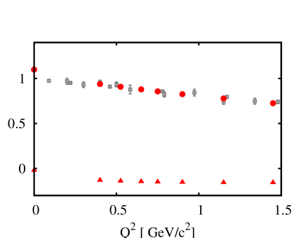
Figure 5: The magnetic $N$-$\Delta$ (1232) transition form factor $G^{*}_{M}(Q^{2})$ defined in Ref.sl96 . $G_{D}=1./(1+Q^{2}/b^{2})^{2}$ with $b^{2}=0.71$ (GeV/c)². The solid circles (solid triangles) are the real (imaginary) parts of our results. The other data points are from previous analysisndff-data .

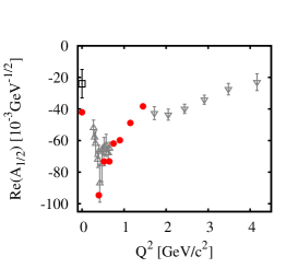
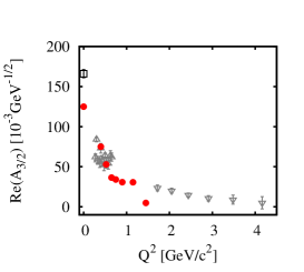
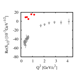
Figure 6: The solid circles are the real parts of the extracted $\gamma N\rightarrow N^{*}(D_{13}(1520))$ form factors. The data are from CLAS collaborationinna . transition form factors

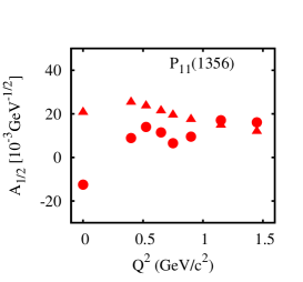
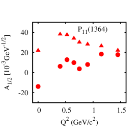
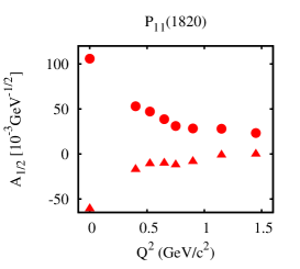
Figure 7: The extracted $\gamma N\rightarrow N*(1356),N*(1364),N*(1820))$ transition form factors of $P_{11}$. The solid circles (solid triangles) are their real (imaginary) parts.

References

- (1) N. Suzuki, T. Sato and T. -S. H, Lee, Phys. Rev. C79, 025205 (2009).
- (2) A. Matsuyama, T. Sato, and T. -S. H. Lee, Phys. Rept. 439, 193 (2007).
- (3) N. Suzuki, B. Julia-Diaz, H. Kamano, T.-S. H. Lee, A. Matsuyama, and T. Sato, arXiv:0909.1356[ncl-th], submitted to Phys. Rev. Lett (2009).
- (4) B. Julia-Diaz, T. -S. H. Lee, A. Matsuyama, and T. Sato, Phys. Rev. C76, 065201 (2007).
- (5) H. Kamano, B. Julia-Diaz, T. -S. H. Lee, A. Matsuyama, and T. Sato, Phys. Rev. C79, 025206 (2009); H. Kamano, B. Julia-Diaz, T. -S. H. Lee, A. Matsuyama, and T. Sato, arXiv:0909.1129 [nucl-th].
- (6) B. Julia-Diaz, T. -S. H. Lee, A. Matsuyama, T. Sato and L. C. Smith, Phys. Rev. C77, 045205 (2008).
- (7) B. Julia-Diaz, H. Kamano, T. -S. H. Lee, A. Matsuyama, T. Sato and N. Suzuki, Phys. Rev. C80, 025207 (2009).
- (8) L. A. Copley, G. Karl, and E. Obryk Nucl. Phys. B13, 303 (1969).
- (9) C. Amsler et al., Phys. Lett. B667, 1 (2008).
- (10) R.A. Arndt, J. M. Ford, L. D. Roper, Phys. Rev. D32, 1085 (1985).
- (11) R.E. Cutkosky and S. Wang, Phys. Rev. D. 42, 235 (1990); R. E. Cutkosky, C. P. Forsyth, R. E. Hendrick and R. L. Kelly, Phys. Rev. D20, 2839 (1979).
- (12) R. A. Arndt, W. J. Briscoe, I. I. Strakovsky, and R. L. Workman, Phys. Rev C74, 45205 (2006).
- (13) Döring M, Hanhardt C, Huang F, Krewald S and Meißner U -G, arXiv:0903.1781 [nucl-th]; Döring M, Hanhardt C, Huang F, Krewald S and Meißner U -G, Nucl. Phys. A829, 170 (2009).
- (14) R. J. Eden and J. R. Taylor, Phys. Rev. Lett. 11, 516 (1963).
- (15) M. Kato, Ann. Phys. (N.Y.) 31, 130 (1965).
- (16) D. Morgan and M.R. Pennington, Phys. Rev. Lett. 59, 2818 (1987).
- (17) R. A. Arndt, W. J. Briscoe, I. I. Strakovsky, and R. L. Workman, Phys. Rev. C66, 055213 (2002); R. A. Arndt, I. I. Strakovsky, and R. L. Workman, Phys. Rev. C53, 430 (1996).
- (18) J. Ahrens et al., Eur. Phys. J. A21, 323 (2004); J. Ahrens et al., Phys. Rev. Lett, 88, 232002 (2002).
- (19) M. Dugger et al., Phys. Rev. C76, 025211 (2007).
- (20) G. Blanpied et al., Phys. Rev. C64, 025203 (2001).
- (21) T. Sato and T. -S. H. Lee, Phys. Rev C54, 2660 (1996).
- (22) W. Bartel et al.,Phys. Lett 28B, 148 (1968); K. Bätzner et al., Phys. Lett. 39B, 575 (1972); J. C. Alder et al., Nucl. Phys. B46, 573 (1972); S. Sterin et al., Phys. Rev. D12, 1884 (1975).
- (23) G. Aznauryan,V,D. Burkert, et al. (CLAS Collaboration), arXiv:0909.2349v2; V.I. Mokeev, V.D. Burkert et al. arXiv:0906.4081.