I: Abstract

I report on the development of new code to support the Nasmyth and E-W antenna mount types in AIPS which will allow polarisation analysis of observations made using these uncommon antenna configurations. These mount types will probably become more widely spread as they have several advantages, particularly for geodetic observatories. Multi-band observations, with multiple receivers, can only be fitted into telescopes with Nasmyth feeds. These are the requirements for the new generation of geodetic arrays as discussed in IVS2010. Further more the next generation of antennae will also be required to have very high slew rates, and these can be achieved with the E-W mount.

The mount type affects the differential phase between the left and the right hand circular polarisations (LHC and RHC) for different points on the sky. The target antennae for the project is the Yebes 40m telescope, but as that is still under construction the data used as a demonstration was from the Pico Veleta antenna as part of the Global Millimeter VLBI Array (GMVA). For the E-W mount type there are suitable data from the Australian LBA array. I have demonstrated the effectiveness of the changes made and that the Nasmyth and E-W corrections can be applied.

This report does not cover the basics of interferometry, nor regular polarisation calibration. For references on these topics see, for example, Thompson, Moran, and Swenson (2001) and Aaron (1997).

II: Observations of polarisation

Why try to recover the polarisation of an observed radio source? Primarily because it often yields unique information about the source. Polarisation is a tracer of asymmetry in the source of radiation, and the most common source of induced asymmetry is the magnetic fields. ‘Seeing’ the magnetic fields around a source of interest provides huge insights into the source emission generation, history and orientation in space. See for example figure 1 of the Pulsar Wind Nebula (PWN) around the Vela pulsar (Dodson etal 2003) where the magnetic field, generated by the particles spewing from the pulsar poles, curves around the pulsar and is stretched back by the pulsar’s motion through the Interstellar medium (ISM).

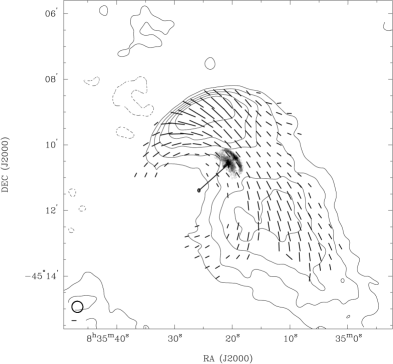
Figure 1: The Chandra observation of the Vela PWN (grey scale) and, superimposed, the 5 GHz Radio contours (-1,1,2,3,4,5 mJy/beam with $20^{\prime\prime}$ beam). The derotated magnetic field lines are overlaid, with a 1 mJy bar at the bottom left, below the restoring beam size. The proper motion vector shows the distance travelled in 1000 years, and ends with the three sigma error ellipse. The field lines confirm that the radio PWN is created by the pulsar, and also show the distortion from the motion of the pulsar.

Instrumental distortion of the polarisation is usually much greater than the inherent signal itself. Polarisation calibration requires the highest standards of general calibration, and it is this which makes it difficult. I focus in this report only on the requirements to correct the new types of telescope mounts. For a summary of the reasons to observe polarisation and the methods see, for example, Ojha (2001).

III: Telescope Mounts

Mount types are a combination of the focus position and the drive type. In Radio Astronomy there are six more or less commonly used focus positions, and three drive types.

III:.1 Focus positions

Radio telescopes use a much more limited set of focus positions compared to optical telescopes. Here we list them, along with examples of the codes for telescopes which use them (in brackets). Images of these are shown in figure 2 and a general schematic is shown in figure 3.

• Prime focus (PKS/MED). Focus at the site of the secondary mirror (sub-reflector).

• Cassegrain focus (VLBA/most). Focus after the secondary (hyperboloid) mirror.

• Gregorian focus (EFF). Prime Focus before the secondary (ellipsoid) mirror, secondary focus after the secondary mirror.

• Folded Cassegrain focus (CED). Focus bolted to the elevation axis, after the tertiary mirror.

• Reduced Nasmyth focus (JCMT). Focus on the elevation axis, but bolted to the azimuth floor, after the tertiary mirror.

• Full Nasmyth focus (PV/YEB40). Focus bolted to the azimuth axis floor, after the forth mirror.

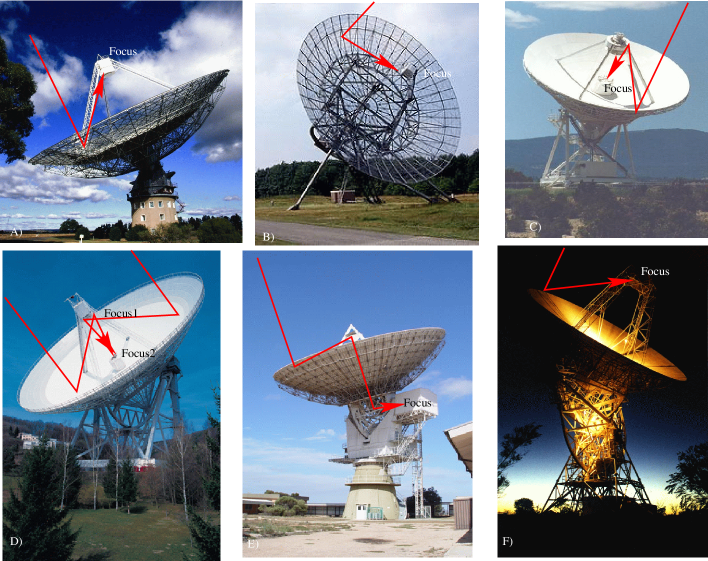
Figure 2: A montage of different antennae displaying different focus positions and drive types. A) Parkes (NSW, Australia). Prime focus, Alt-Az drive, B) Westerborg (Holland). Prime focus, HA-Dec drive. C) Los Alamos (USA). Cassegrain focus, Alt-Az drive. D) Effelsberg (Germany) Either Prime or Gregorian focus, Alt-Az drive. E) Ceduna (SA. Australia). Folded Cassegrain focus, Alt-Az drive. F) Hobart (TAS Australia) Prime Focus, EW drive.

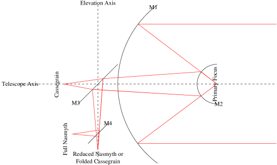
Figure 3: Mount types

Mirrors after the forth, in a Nasmyth system, swap the mount type between the equivalent of a reduced and full Nasmyth, so that any system with an odd number of mirrors is a ‘reduced’ and an even number of mirrors is equivalent to a ‘full’ Nasmyth system in our context. In a similar fashion the expression for a folded Cassegrain and Prime focus solutions are essentially the same, being either one or three reflections from the on-sky view. The difference between a Cassegrain and a Gregorian image is a rotation (of 180^o) so these types are degenerate after the absolute position angle calibration. Furthermore at the correlator, the ‘on sky’ left or right is combined with the same to produce the parallel hand output. This is effectively the same as adding another mirror to the optical chain for those optics with an odd number of mirrors. For all expected cases, therefore, we will be correlating either Cassegrain or Nasmyth foci, combined with the drive type of the antenna. The other possibilities were tested and included in the development code. They maybe of use for single dish analysis, but it is not planned to include them in standard AIPS.

III:.2 Drive configuration

There are three drive configurations used in VLBI. This also effects the rotation of the feeds as seen from the sky.

• HA-DEC (WST), for Hour Angle – Declination. Also called equatorial. It produces no change of feed angle as the source passes across the sky. As HA-DEC mounts require an asymmetrical structural design they are unsuited to the support of very heavy structures. Their advantage is that motion is required in only one axis to track an object as Earth rotates.

• ALT-AZ (VLBA/most), for Altitude – Azimuth. Also called Az-El. It rotates the telescope pointing by the parallactic angle as the source passes across the sky. It is the most common variety of Radio telescope mount. It is symmetric so can support very large antennae, but at the zenith small angular changes on the sky can require very large angular changes in the azimuth angle. This effect is call the ‘keyhole’.

• EW (HOB), for East – West. It rotates the telescope by the co-parallactic angle as the source passes across the sky. An EW mount places the focus very high, therefore it is prone to flexing and poor pointing. Their advantage is that they can track across the sky at high speeds and without gaps (i.e. it does not have a ‘keyhole’ at the zenith). They are primarily used for tracking Low Earth Orbit satellites.

The parallactic angle, sometimes called the position angle, of an object is the angle between the celestial pole (north or south depending on location), the object and the zenith (the point in the sky directly overhead). It is not to be confused for the same named angle which is also called the convergence angle. This is the difference in the angular direction to an object at a distance, from two points of view, i.e. the parallax. The expression for the parallactic angle as we use it is;

$$\chi_{p}={\rm arctan}[\frac{{\rm sin}(\Theta)\ {\rm cos}(l)}{{\rm cos}(\delta){\rm sin}(l)-{\rm cos}(\Theta){\rm cos}(l){\rm sin}(\delta)}]$$

The co-parallactic angle is;

$$\chi_{c}={\rm arctan}[\frac{{\rm cos}(\Theta)}{{\rm sin}(\delta){\rm sin}(\Theta)}]$$

The Nasmyth angle is almost the same as the parallactic angle, but with the relative rotation of the third mirror included;

$$\chi_{n}=\chi_{p}\pm E$$

where $\Theta$ is the hour angle, and $\delta$ the declination, of the source. $l$ is the latitude of the telescope and $E$ is the elevation. These angles are calculated in the code using the function atan2 to allow the full range of angles to be returned.

IV: The Nasmyth Mount

The feed in a Nasmyth system sits within the Azimuth cabin of an Alt-Az telescope. Therefore the difference between the instrumental polarisation angle of a Nasmyth mount and the parallactic angle is the elevation angle. Consider the change in the image of the secondary reflector projected onto the feed mount. At the horizon it has the correct orientation, and is rotated as the telescope moves in elevation. The sense of the rotation is positive (clockwise) or negative (counter-clockwise) depending on whether the M3 (see figure 3) reflects to the right or left. The secondary reflector follows the parallactic angle (assuming the drive type is an Alt-Az). Each mirror adds a swap of polarisation from LHC to RHC. Therefore, in principle, the number of reflections before the horn is very important in a Nasmyth optical system, as each mirror also swaps the feed angle polarisation vector on the sky. However when the detected LHC or RHC polarisations are relabelled to represent the on-sky value, an effective mirror is added to produce the parallel or cross hand outputs. This means that the ‘reduced Nasmyth’ (and the ‘prime focus’) case(s) should never be met in the real world in VLBI. It maybe necessary if AIPS is used for single dish reduction. Nevertheless, the extension of the test version of AIPS to handle all varieties of Nasmyth (three), Prime Focus and EW mount types was done in parallel. The version which will be merged with the standard AIPS will not include the extra code.

V: The basic equations for the solution of polarisation

There are numerous sources of information laying out the methods for reducing polarisation observations. One of the best is EVN Memo 78 (Aaron, 1997), but also see Kemball (1999), Ojha (2001), Leppanen etal (1995) and Hamaker (2000). All of these are for telescopes where the feed angle is implicitly the parallactic angle (or possibly also the equatorial angle). If one replaces all occurrences of the term ‘parallactic angle’ with the more generic ‘feed angle’ these are all correct. From these references we repeat only the derivation of the D-term equations.

For an ideal case (i.e. unitary gain, no cross talk and no on-sky feed rotation) the observables are:

$$R_{1}R_{2}=(I_{12}+V_{12})$$

$$L_{1}L_{2}=(I_{12}-V_{12})$$

$$R_{1}L_{2}=(Q_{12}+iU_{12})=P_{12}$$

$$L_{1}R_{2}=(Q_{12}-iU_{12})=P^{*}_{12}$$

Where R and L are Right and Left handed polarisations, I, Q, U and V are the stokes parameters, and P is the linearly Polarised flux.

But when we have gain terms ($g$), cross talk ($R_{obs}=R+DL$), and feed rotation ($\chi$) this becomes, for example;

$$\begin{array}[]{lr}R_{1}L_{2}=<E_{R_{1}}E_{L_{2}}^{*}>=&g_{R_{1}}g^{*}_{L_{2}}[P_{12}e^{-i(\chi_{1}+\chi_{2})}+\\ &D_{R_{1}}D^{*}_{L_{2}}P^{*}_{12}e^{i(\chi_{1}+\chi_{2})}+\\ &D_{R_{1}}L_{1}L_{2}e^{i(\chi_{1}-\chi_{2})}+\\ &D^{*}_{L_{2}}R_{1}R_{2}e^{-i(\chi_{1}-\chi_{2})}]\end{array}$$

Where $g$ is the complex gain, $\chi$ the phase from feed angle, and $D$ the D-terms. However, assuming $V=0$ (i.e. zero circular polarisation), and that small terms (e.g. $D^{2}$) tend to zero, we can simplify to:

$$R_{1}R_{2}=g_{R_{1}}g_{R_{2}}^{*}Ie^{-i(\chi_{1}-\chi_{2})}$$

$$L_{1}L_{2}=g_{L_{1}}g_{L_{2}}^{*}Ie^{+i(\chi_{1}-\chi_{2})}$$

$$R_{1}L_{2}=g_{R_{1}}g_{L_{2}}^{*}[Pe^{-i(\chi_{1}+\chi_{2})}+D^{*}_{L_{2}}RRe^{-i(\chi_{1}-\chi_{2})}+D_{R_{1}}LLe^{i(\chi_{1}-\chi_{2})}]$$

$$L_{1}R_{2}=g_{L_{1}}g_{R_{2}}^{*}[P^{*}e^{i(\chi_{1}+\chi_{2})}+D^{*}_{R_{2}}LLe^{+i(\chi_{1}-\chi_{2})}+D_{L_{1}}RRe^{-i(\chi_{1}-\chi_{2})}]$$

Assuming that $P$ is a constant fraction of $I$ ($P=pI$), and $RR=LL=I$ (as $V=0$), and exchanging $g{{}^{\prime}}_{R_{m}}$ for $g_{R_{m}}e^{-i\chi_{m}}$ and $g{{}^{\prime}}_{L_{m}}$ for $g_{L_{m}}e^{+i\chi_{m}}$ we get;

$$R_{1}R_{2}=g{{}^{\prime}}_{R_{1}}g{{}^{\prime}}_{R_{2}}^{*}I;L_{1}L_{2}=g{{}^{\prime}}_{L_{1}}g{{}^{\prime}}_{L_{2}}^{*}I$$

$$R_{1}L_{2}=g{{}^{\prime}}_{R_{1}}g{{}^{\prime}}_{L_{2}}^{*}I(p+D^{*}_{L_{2}}e^{2i\chi_{2}}+D_{R_{1}}e^{2i\chi_{1}}]$$

$$L_{1}R_{2}=g{{}^{\prime}}_{L_{1}}g{{}^{\prime}}_{2_{2}}^{*}I(p^{*}+D^{*}_{R_{2}}e^{-2i\chi_{2}}+D_{L_{1}}e^{-2i\chi_{1}}]$$

The polarisation calculation is based on the fit of the cross to parallel flux ratios: e.g. $RL/RR$. These are:

$$RL/RR=\frac{g{{}^{\prime}}_{L_{2}}g{{}^{\prime}}_{R_{1}}I}{g{{}^{\prime}}_{R_{2}}g{{}^{\prime}}_{R_{1}}I}(p+D^{*}_{L_{2}}e^{2i\chi_{2}}+D_{R_{1}}e^{2i\chi_{1}})$$

$$=pe^{-2i\chi_{2}}+D^{*}_{L_{2}}+D_{R_{1}}e^{2i(\chi_{1}-\chi_{2})}$$

similarly,

$$LR/RR=p^{*}e^{2i\chi_{1}}+D_{L_{1}}+D^{*}_{R_{2}}e^{2i(\chi_{1}-\chi_{2})}$$

$$RL/LL=pe^{-2i\chi_{1}}+D_{R_{1}}+D^{*}_{L_{1}}e^{-2i(\chi_{1}-\chi_{2})}$$

$$LR/LL=p^{*}e^{2i\chi_{2}}+D^{*}_{R_{2}}+D_{L_{1}}e^{-2i(\chi_{1}-\chi_{2})}$$

A final enhancement is that P, the polarised emission, can be modeled as polarised fractions of subsections of the total emission. That is;

$$P=\Sigma_{n}p_{n}I_{n}$$

This is the formalisation used in the AIPS task LPCAL, and is why LPCAL is to be preferred for VLBI polarisation calibration.

VI: Formulation in terms of Jones matrices

Jones Matices are a very useful way to express the optical chain. The usual formalisation, and the one used here is for the X and Y (Elevation and Azimuth) axes.

A mirror (reflecting from left to right) is:

$$M=\left(\begin{array}[]{rr}1&0\\ 0&-1\end{array}\right)$$

A rotation of $\theta$ (where $\theta$ is the elevation in the Nasmyth case) is:

$$R=\left(\begin{array}[]{rr}cos(\theta)&sin(\theta)\\ -sin(\theta)&cos(\theta)\end{array}\right)$$

The complex D-terms are:

$$D=\left(\begin{array}[]{cc}1&D_{x}\\ D_{y}&1\end{array}\right)$$

For the case of a Full Nasmyth antenna the Jones matrices include the Cassegrain terms from the ‘structure’ (following the parallactic angle) $D_{C}$ and the Nasmyth terms from the ‘feeds’, $D_{N}$. The resultant optical chain is equivalent to:

$$\equiv(M_{n}\cdots M_{5})\cdot D_{N}\cdot M_{4}\cdot R(t)M_{3}\cdot[D_{C}\cdot M_{2}\cdot M_{1}]$$

From this formulation it is clear that the $D_{N}$ and $D_{C}$ can not be combined, as they are either side of the time varying rotation matrix. Furthermore is obvious that if there is a final number of odd mirrors the solution is equivalent to a reduced Nasmyth system, and the full Nasmyth applies to the case with an even number of mirrors. But recall that exchanging the labels of LHC and RHC to reflect the on-sky polarisation is the equivalent to yet another mirror. Finally that the D-term solutions will swap (to their negated conjugate) in each mirror, if the calibrator is unpolarised (or assumed to be unpolarised). The expression in square brackets is that for a Cassegrain system.

VII: Contributions to the D-terms

D-terms arise from the cross talk of the nominally right hand circular feed to the nominally left hand circular feed (or X and Y linear feeds, which are not relevant to the discussion here). Three dominant mechanisms for cross talk exist: i) Elliptical feeds: In practice linear probes are used to detect the incoming wave, therefore a quarter wave plate is placed in front of these feeds to convert the incoming circular polarisation to linear polarisation. A quarter wave plate is only perfect at a single frequency, and even then only if perfectly constructed. Therefore the conversion will always produce a certain amount of ellipticity which is tied directly to the receiver; ii) Impedance-matching: The feeds will not be perfectly impedance-matched to the incoming system, so there will be a certain amount of power re-emitted from each probe. This power can then be reflected back into the receiver, with the circular polarisation swapped, and this reflection can be from anywhere in the optical system. This is not normally an issue, as long as they are constant in time, as these D-terms are degenerate with those of the receiver. In a Nasmyth antenna this is not true for reflections returning from the M2 mirror as there is a time varying rotation at this point; iii) Pointing offsets: Even a perfect system has intrinsic D-terms away from the symmetry axis (because of the loss of symmetric cancellation of terms). These are inextricably tied to the Alt-Az mount through the sub-reflector (M2), and in principle could change with time. These, if significant, will have to be solved for using the Az-Alt mount type, see Brisken (2003) for the eVLA analysis. However modeling at Yebes (F. Tercero, personal comm.), particularly for the SX receiver package, has suggested that the level of cross talk will be less than 0.1%. These levels, if correct, will be undetectable. Time varying D-terms would require unpolarised calibrators as is impossible to get good parallactic angle coverage in short time spans. The Left-Right ‘beam squint’ also is a contributor to off axis polarisation for the VLA. In the usual VLBI case, because the fields of view is so much smaller, it does not contribute. The Left-Right gains are solved for at the pointing centre and no imaging is attempted significantly far from this point. However, for wide field VLBI imaging, it will become an issue. In this case amplitude calibration would need to be performed at each imaging centre.

The need for double D-terms are conceivable, therefore we have developed test code and a method to allow combined Nasmyth and Cassegrain D-term solutions. It is not clear that the secondary terms will be necessary in any ‘real-world’ example.

VIII: Double D-terms

Returning to the expressions for the cross hands with D-terms for two kinds of rotation we find:

$$\begin{array}[]{lllll}R_{1}L_{2}=&g_{R_{1}}g_{L_{2}}^{*}[Pe^{-i(\chi_{1}+\chi_{2})}&+\\ &D^{*}_{L_{2}}RRe^{-i(\chi_{1}-\chi_{2})}&+&D^{\prime*}_{L_{2}}RRe^{-i(\chi_{1}-\Theta_{2})}&+\\ &D_{R_{1}}LLe^{i(\chi_{1}-\chi_{2})}&+&D^{\prime}_{R_{1}}LLe^{i(\Theta_{1}-\chi_{2})}&~{}]\end{array}$$

$$\begin{array}[]{lllll}L_{1}R_{2}=&g_{L_{1}}g_{R_{2}}^{*}[P^{*}e^{i(\chi_{1}+\chi_{2})}&+\\ &D^{*}_{R_{2}}LLe^{+i(\chi_{1}-\chi_{2})}&+&D^{\prime*}_{R_{2}}LLe^{+i(\chi_{1}-\Theta_{2})}&+\\ &D_{L_{1}}RRe^{-i(\chi_{1}-\chi_{2})}&+&D^{\prime}_{L_{1}}RRe^{-i(\Theta_{1}-\chi_{2})}&~{}]\end{array}$$

Where $\chi$ is the feed angle, and $\Theta$ is the extra (parallactic angle) term, and $D^{\prime}$ is the $D$ term associated with this extra term.

This, after the feed angle correction, reduces to:

$$R_{1}L_{2}=g{{}^{\prime}}_{R_{1}}g{{}^{\prime}}_{L_{2}}^{*}I(p+D^{*}_{L_{2}}e^{2i\chi_{2}}+D_{R_{1}}e^{2i\chi_{1}}+D^{\prime*}_{L_{2}}e^{i(\Theta_{2}+\chi_{2})}+D^{\prime}_{R_{1}}e^{i(\Theta_{1}+\chi_{1})}]$$

$$L_{1}R_{2}=g{{}^{\prime}}_{L_{1}}g{{}^{\prime}}_{2_{2}}^{*}I(p^{*}+D^{*}_{R_{2}}e^{-2i\chi_{2}}+D_{L_{1}}e^{-2i\chi_{1}}+D^{\prime*}_{R_{2}}e^{-i(\Theta_{2}+\chi_{2})}+D^{\prime}_{L_{1}}e^{-i(\Theta_{1}+\chi_{1})}]$$

The easiest way to investigate this effect was to allow the fitting of dual terms – but only to apply one. A second pass of LPCAL would then allow the application of the other term, with the other feed angle. Therefore, in the code (LPCAL_EXT) only one “double termed” antenna.

IX: AIPS code changes

The fundamental alteration was to add support for the Nasmyth optics (and EW-mount optics). The core subroutine for the calculation of parallactic angles was extended to return either, the parallactic plus or minus the elevation angles, or co-parallactic angles (i.e. the correct formalisation for these mount types). In addition test code was written for reduced Nasmyth and Prime focus mount types. The mount types, and their numeric values, are listed in table 1.

		Mount Number
Focus and Drive	Label	Test	Final
Cassegrain and Alt-Az	ALAZ	0	0
Any and Equatorial	EQUA	1	1
Any and Orbiting	ORBI	2	2
New mount types
Prime focus and EW	EW- -	$\pm$3	3
Right hand Naysmyth and Alt-Az	NS-R	4	4
Left hand Naysmyth and Alt-Az	NS-L	-4	5
Extra mount types
Reduced Nasmyth and Alt-Az	R-NS	$\pm$5	-
Prime focus (or Folded Cassegrain) and Alt-Az	PRIM	6	-

Table 1: Mount Types

The extra mount types will not be carried forward for inclusion in to AIPS, as they are only for testing.

All calls to this code have been checked, as have all calls to the mount type via GETAN, all mentions of “parallactic” in the source code, and all mentions of any of the common names for mount type (MNTYP, MNTSTA, MNTEL and IDTMNT). All issues associated with those have been fixed. A full list of the differences can be found in appendix B.

The greatest problem was that not all derivations of the parallactic angle were done with a single common subroutine. This was fixed for most cases, but in one case it has not been standardised, i.e. VPLOT (for which one can use UVPLT). In VPLOT the position angle is only used as an alternative plotting axis, and therefore has no impact on the data reduction.

A point of concern is that these corrections are for a ‘moving target’. The code written was for the 31DEC05 version of AIPS downloaded in February 2005. There have been considerable changes since that date. The latest version was for the January version of 31DEC07. It is highly desirable that the new code is merged with the distribution tree.

X: Data visualisation

The first stage of calibration is to correct the relative phase rotation between the left hand and the right hand receivers. The success of this stage can be easily demonstrated with the task VPLOT by plotting the phases difference between the two polarisations (usually against time). The phase of the ratio of the parallel hands will be, before feed angle calibration;

$$\frac{R_{1}R_{2}}{L_{1}L_{2}}=\frac{g_{R_{1}}g_{R_{2}}^{*}}{g_{L_{1}}g_{L_{2}}^{*}}e^{-i(\chi_{1}-\chi_{2})}$$

and after;

$$\frac{R_{1}R_{2}}{L_{1}L_{2}}=\frac{g{{}^{\prime}}_{R_{1}}g{{}^{\prime}}_{R_{2}}^{*}}{g{{}^{\prime}}_{L_{1}}g{{}^{\prime}}_{L_{2}}^{*}}$$

Therefore the phases between the two polarisations, post feed angle calibration, will have a constant phase. See figure 6. Post phase calibration, of course, this phase will be zero. This step is in theory independent of any other calibration but in practice, as the data is averaged then compared, the delays need to be solved for and the VPLOT averaging has to be less than the (post-calibration) coherence time. That is, either short averaging intervals must be used (with the risk that the phase difference will be undetectable) or at least some phase calibration must have been performed. It is important that, in this case, the phases applied to each polarisation are not independent. Otherwise the effect is masked as the phases are absorbed into the calibration. Examples of these RR/LL plots are to be found in figures 6 and 12.

Conventionally the quality of the polarisation solutions was judged from plotting RL/RR (or LR or against LL) on the real/imaginary plane with and without polarisation calibration. Without calibration the values will fall on a circle around an (offset and potentially moving) origin, as a function of feed angle difference, following:

$$RL/RR=pe^{-2i\chi_{2}}+D^{*}_{L_{2}}+D_{R_{1}}e^{2i(\chi_{1}-\chi_{2})}$$

I.e. if the source is unpolarised ($p=0$), the centre is $D^{*}_{L_{2}}$ and the radius of the circle is $D_{R_{1}}$. Examples of such plots are to be found in figure 4 etc. This is a useful diagnostic tool, but it can be improved on. I added code to LPCAL which allows the interactive plotting of the data, with and without the model fitted removed, against many other data axes, see figure 5.

The extended data visualisation is done via a PGPLOT X-window interface added into LPCAL. Therefore LPCAL needs to be compiled with extra options. This is not planned to become part of classic AIPS but can be requested. The data is plotted (as coloured points) in several forms with the model overlaid (as coloured lines). The residuals are displayed in a subplot. See Figure 5. Plots of RL or LR data, can be on the complex plane or against data index or feed angle. Either the absolute, real or imaginary data can be plotted. Individual antennas can be selected, or overlaid.

X:.1 Commands

• Data Plane: Complex (c), feed Angle (a) or array Index (i)

• Data product: RightLeft (r) or LeftRight (l)

• Data Value: Absolute (1), Real (2) or Imaginary (3)

• quit (q)

Extras:

• Site selection (s followed by number).
  When greater than 9 use + and number (i.e. s+1 for 11). (Tip: s++ increments antenna number by 1)

• Model on or off (m)

• Differential value (d) (i.e. $\chi_{i}-\chi_{j}$ for feed angle, or baseline index rather than total index)

• Zoom: Top corner (t) and Bottom corner (b). Reset with new data

• Plot: a colour postscript (pgplot.ps) file is generated (p) of the current viewing plane.

Figure 4: Pre- and Post- polarisation solution from traditional VPLOT display for the four antennae in V148A.

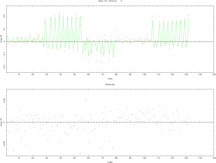
Figure 5: Solutions for Ceduna in experiment V148A displayed via the new interactive visualisation subroutines. The shown visualisation mode is showing imaginary RL flux (in Jy) against baseline and time (index). The upper window shows the data (in red points) and the model (with a green line) and the lower shows the residuals. For each integration period the data for each baseline involving the selected antenna (number 4, Ceduna) is plotted.

X:.2 Comments

The Index data plane, which I personally find most useful, will usually represent the data in the “TB” sort order. This leads to the raggedy appearance, as each baseline is looped over for every time index. Altering the order to “BT” would remove this effect, but LPCAL does not work on BT ordered data. No solution for this has been identified.

The Zoom needs to be selected from the lower plot. The default limits come from the maximum and minimum of the entire dataset. With a SOLINT of 1 minute this produces a great scatter.

XI: Demonstration of a conventional VLBI data analysis

It is important to confirm that our changes have not broken the AIPS system. I have use the VLBA data set BR046. The Figures 7 show the solutions. We find the same solutions as those derived on a vanilla AIPS installation, plus on the target and calibration sources (to within errors). Furthermore we find that the solutions are robust when derived from the other source, and with the assumption of an unpolarised point source. We conclude that the changes are non-toxic.

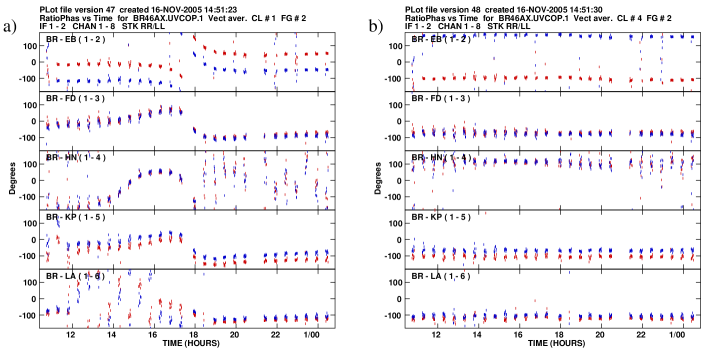
Figure 6: Plots demonstration the successful correction of the differential phase rotation of the two parallel hands for experiment BR046. a) is pre-calibration and b) is post calibration.

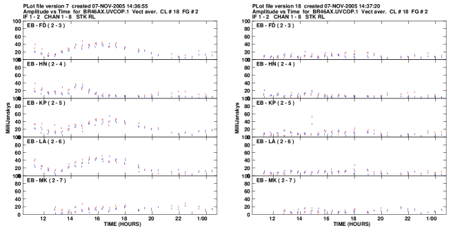
Figure 7: Selected plots from the task VPLOT showing the successful polarisation calibration of experiment BR046. The pre polarisation calibration is shown on the left for a number of telescopes to Effelsberg. Post calibration is on the right. Note that the magnitude of the flux in the cross hands falls, and becomes constant with time.

Furthermore we analysed the EVN dataset N05L1, a network monitoring experiment. This included OQ208 which is unpolarised, and therefore could be used as a calibrator despite the short length (and therefore poor parallactic angle coverage) of the experiment. In this dataset of thirteen antennas there were three antenna with prime foci and two with equatorial mounts. The best solutions were found following the conventional analysis (as would be expected), but we also tested the reduction with the prime focus mount type.

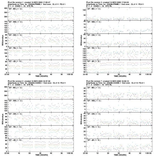
Figure 8: Selected plots from the task VPLOT showing the successful polarisation calibration of experiment NL051. The pre polarisation calibration is shown on the left for a number of telescopes to Effelsberg. Post calibration is on the right. The upper plots are for analysis with the PRIME focus used for Effelsberg, Medicina and Jodrell Bank, the lower used the nominal mount types. The solutions based on the nominal types are significantly better.

XII: Investigations of Prime Focus, Folded Cassegrain and EW-mount VLBI data analysis

This required the extra step of installing ATLOD to AIPS. It is required for all tasks involving the Australian CSIRO “Radio Physics Fits” (RPF) format. I used the experiment LBA data set V148. This experiment of a 6.7 GHz polarisation experiment with Parkes (Prime focus), ATCA and Mopra (Cassegrain), Ceduna (Folded Cassegrain) and Hobart (E-W mount). It was in two session (A1+A2 and B) and included seven scans each of two polarisation calibrators (1610-771 and 1718-649) which allowed the demonstration that:

• The additional mount types did not effect the conventional mounts.

• That the zeroth order Nasmyth (the folded Cassegrain) and the Prime focus have D-terms that are negated and conjugated if they are treated as a conventional Cassegrain system.

• That the number of antennae needs to be greater than three to also solve the polarised fraction of the source .

• That the antennae Mopra, Parkes and ATCA have very similar parallactic angles, and therefore the solutions with just these maybe degenerate. The addition of (sufficient) additional antennae breaks this degeneracy.

Dataset V148A raised some interesting questions as stable solutions are only found when Parkes is treated as a prime focus and Ceduna as (the equivalent) folded Cassegrain. This contradicts the results from the EVN (where Effelsberg is a prime focus, but the most stable solutions were found when it was treated as a Folded Cassegrain (i.e. the sign reversed) feed). No explanation was found for this, and as reasonable solutions were found for the conventional analysis, we decided this was an unexplained distraction which maybe related to the limited number of antennae.

V148B behaved in a more sensible manor, and we note that this dataset has one additional antenna (Hobart) which might be providing enough to break the degeneracy. This underlines the importance of the EW mount type code; without it the (usual) LBA has insufficient differential parallactic angle coverage. Figure 9 shows the comparison of the position angles found from the V148B experiment and those from an ATCA observation of the same source. They agree very well, with the added benefit of the VLBI observations resolving separate components and allowing better polarised flux recovery. The polarised flux found in the VLBI observations between -35 and -36 kms^-1 have, in fact, better recovery of polarised flux then the ATCA which does not show up in the imspec generated plots. These velocities are the overlap region between the Eastern and Western clusters, so the lower resolution of the ATCA is blending these and thus not detecting the polarisation.

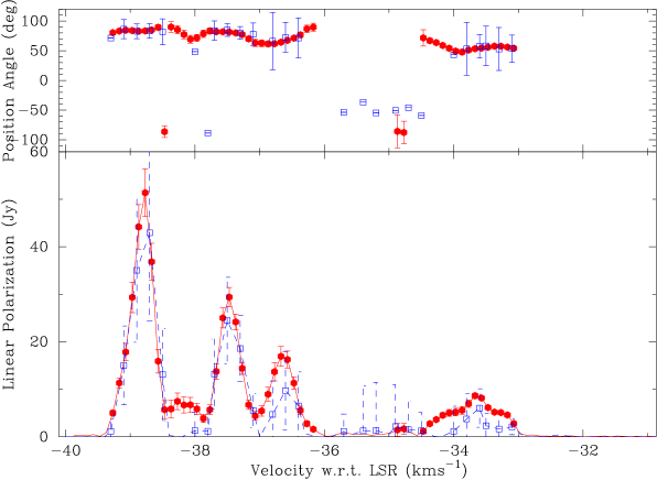
Figure 9: Polarisation angle and fraction for G339-1.26, as observed by the LBA (this paper, blue open squares) and the ATCA (Ellingsen, priv. comm., red closed circles). The spectra is scalar summed across the image (Stokes I,Q and U), and shows good agreement between the VLBI and the connected array results. The errors are the absolute errors based on the confidence in the polarisation calibration (2% and 0.4% respectively), not the relative errors. Where errors are not shown they could not be calculated. From Dodson, 2007

XIII: D-terms for experiment V182A

This experiment (PI Dr Dodson) was performed on the LBA at 4.8 GHz with 64 channels of about 0.25 MHz each. The target source (J0743-67) is an AGN with an interesting double structure. The calibrator was J0637-752, also an interesting source. It is the first experiment to produce solutions for the polarisation on the LBA, but was not designed as a polarisation experiment, therefore it does not include a absolute polarisation calibrator and all position angles are arbitrary. It included Hartebeesthoek so had more baselines to solve for amplitude and D-terms. Reduction followed the standard routes, apart from changing the mount types to EW mount for Hobart and equatorial mount for Hartebeesthoek.

Figure 10: The RR/LL phase difference in LBA experiment V182A before and after feed angle correction types. The mount types are parallactic and equatorial and co-parallactic. The phase between the two polarisations before (left) and after removal of the feed rotation in V182A, for all antennae to the CAT. The rotation of the feeds introduces a variable phase between the two hands in the data. The effect of the near identical feed angles for the NSW antenna is indicated by the near constant phases between them. The phases are flattened (and zeroed for the calibrator at 14UT) for all antennae in the corrected data, which is shown on the right.

Figure 11: The image of J0743-67 from experiment V182A. The polarisation vectors are shown overlaid. Absolute polarisation angles can not be derived so the direction is arbitrary. The core (to the West) is unpolarised ($\leq 1\%$) and the jet (to the East) is smoothly polarised with a polarised fraction of approximately 16%.

XIV: Demonstration of a Full Nasmyth optics VLBI data analysis

During the project the only suitable data from the Pico Veleta antenna that was obtained was without any amplitude calibration or flagging tables. Nevertheless I was able to demonstrate the successful correction of the feed angle terms. Three types of correction were applied. Those for Cassegrain feed rotation (mount type 0, or ALAZ) those for the Right-handed Nasmyth feed rotation (mount type 4) and those for left-handed Nasmyth feed rotation (mount type 5). Figure 12 plots the phase difference between left and right hand polarisation for each of these cases, plus the elevation of Pico Veleta at the times of observation. The slope without Nasymth correction is positive, and the opposite of the trend of the elevation, with the incorrect Nasmyth correction the slope is greater, and with the correct terms the phase difference is flat with time. Further analysis of this experiment is impossible, as amplitude calibration cannot be performed and, as stated, that is an essential precondition for good polarisation calibration. This, however, is in itself a complete demonstration of the application of the Nasmyth feed angle expression. Combined with the successful application of other feed angle expressions the calibration pipeline is demonstrated to be complete.

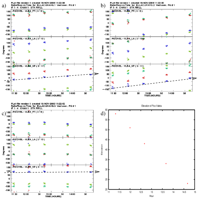
Figure 12: The RR/LL phase difference in GMVA experiment C051A for three parallactic angle correction types: a) Cassegrain, b) Nasmyth right handed and c) Nasmyth left handed. d) Shows the elevation angle for these observation times. The dashed line proves a guide to the eye of phase changes with time. It is obvious that case c) is correct and has flattened the phase response.

Appendix A Recommendations for calibration of polarisation observations

Many references have covered this, but here I wish to clearly layout the important steps in AIPS and the consequences of the tasks.

• TABED options: INE ’AN’; OPTY ’repl’; APARM 5 0 0 4 4 3 and KEYV 5 0
  Replaces the MNTSTA type of antenna 3 with value 5 (for a left handed Nasymth, such as Pico Veleta).
  For Hobart and the LBA this needs to be type 3, furthermore one needs to change for all antenna: columns 8 and 11 to zero (APARM 8/11 0 0 2 0;KEYV 0), column 7 to ’R’ and 10 to ’L’ (APARM 7/10 0 0 3 0;KEYST ’R’/’L’). Recall also that Harts is Equatorial (mntyp 1).

• CLCOR options: CLCORP 1 0 and OPC ’pang’
  Calculates the phase correction for the listed mount types.

• FRING options: CALS ’prime_cal’; APARM(3)=0 and APARM(5)=0
  Finds the independent delays and combined rates and phases for the calibrator. Now the RR/LL phase will be constant.

• CALIB options: CALS ’prime_cal’; SOLMODE ’P’; APARM(3)=0 and APARM(5)=0
  Finds the independent rates and phases for the calibrator. Now the RR, LL and RR/LL phases will be zero. One may wish to use only one scan on the prime calibrator.

• VLBACPOL this procedure finds the delays between left and right hand for the reference antenna. If PCAL (or something similar) is used the delay between left and right should be zero.

• FRING options: CALS ’target’,’calib’; APARM(3)=1 and APARM(5)=1
  Finds the rates and combined phases for the target.

• CALIB options: CALS ’calib’; SOLMODE ’A&P’; APARM(3)=1 and APARM(5)=1
  Produces a well calibrated version of the target which can be imaged.

• IMAGR Deconvolve this with, either a few model components, or clean it and then box up the clean components into a few regions (with CCEDT), and use it for the next stage.

• LPCAL options: CALS ’calib’; in2na ’calib’ and in2c ’icln’
  Does the polarisation calibration on the target, using the cleaned model.

• CALIB options: CALS ’target’; SOLMODE ’A&P’; DOPOL 2; APARM(3)=1 and APARM(5)=1
  Calibrates the target using the polarisation solutions.

• IMAGR Image the source in I, Q and U. The sum of the fluxes (total and polarised) should compare to the lower resolution (VLA or ATCA) values. The correction $\phi_{{\rm RL}}$ is $2\chi_{{\rm true}}-\arctan(\frac{\sum{\rm U}}{\sum{\rm Q}})$, for each IF.

• CLCOR options: CLCORP $\phi_{{\rm RL}}$ stokes ’L’ and OPC ’polr’
  Rotates the D-terms to match the calibration value of $\chi_{{\rm true}}$.

If this recipe is not followed the solutions for the L and R hand polarisations are independent. This is not a problem if there is sufficient signal to noise, however in mm-VLBI this is rarely the case and the two polarisations need to be combined in the fringe search stage. This is why it is important not to treat them as independent except for the prime calibrator.

Appendix B A list of the changes to classic AIPS

A summary of the files changed:

• LPCAL.FOR: Add a new subroutine LPCAL_VIS

• LPCAL_EXT.FOR: New program to allow dual D-terms

• PARANG.FOR: all mount types now supported

• PRTAN.FOR: Add mount names

• CLCOR.FOR: in ANAXIS allow all mount types

• DFCOR.FOR: in ANAXIS allow all mount types

• SNPLT.FOR: does not use PARANG, so mount types added

• DTSIM.FOR: (in ORIENT) does not use PARANG, so mount types added

• DTSIM.FOR: (in GETBAS) allow all mount types

References

- [1] Aaron, S., 1997, EVN Memo #78, “Calibration of VLBI polarisation data”, http://www.jive.nl/techinfo/evn_docs/evn_docs.html
- [2] Brisken, W., 2003, eVLA Memo #58, “Using Grasp8 To Study The VLA Beam”, http://www.aoc.nrao.edu/evla/geninfo/memoseries/evlamemo58.pdf
- [3] Dodson, R. 2007, A&A, submitted
- [4] Dodson, R., Lewis, D., McConnell, D., Deshpande, A. A. 2003. “The radio nebula surrounding the Vela pulsar.” Monthly Notices of the Royal Astronomical Society 343, 116-124.
- [5] Hamaker, J. P. 2000. “Understanding radio polarimetry. IV. The full-coherency analogue of scalar self-calibration: Self-alignment, dynamic range and polarimetric fidelity.” Astronomy and Astrophysics Supplement Series 143, 515-534.
- [6] Leppanen, K. J., Zensus, J. A., Diamond, P. J. 1995. “Linear Polarization Imaging with Very Long Baseline Interferometry at High Frequencies.”Astronomical Journal 110, 2479.
- [7] Kemball, A. J. 1999. “VLBI polarimetry.” ASP Conf. Ser. 180: Synthesis Imaging in Radio Astronomy II, 180, 499.
-
[8]
Ojha, R., 2001, LBA Workshop,
http://www.atnf.csiro.au/rojha/lbapstuff/workhandout_inc.ps - [9] Rioja, M. J., Dodson, R., Porcas, R. W., Suda, H., Colomer, F. 2005, “Measurement of core-shifts with astrometric multi-frequency calibration.”, 17th European VLBI Meeting for Geodesy and Astometry, astro-ph/0505475.
- [10] Thompson, A. R., Moran, J. M., Swenson, G. W. 2001. “Interferometry and Synthesis in Radio Astronomy”, 2nd Edition. Wiley-Interscience