Excitation of coherent polaritons in a two-dimensional atomic lattice

Abstract

We describe a new type of spatially periodic structure (lattice models): a polaritonic crystal (PolC) formed by a two-dimensional lattice of trapped two-level atoms interacting with quantised electromagnetic field in a cavity (or in a one-dimensional array of tunnelling-coupled microcavities), which allows polaritons to be fully localised. Using a one-dimensional polaritonic crystal as an example, we analyse conditions for quantum degeneracy of a low-branch polariton gas and those for quantum optical information recording and storage.

I INTRODUCTION

This work develops the ideas that S.A. Akhmanov paid much attention to in the last years of his life. It addresses the general principles, laid by Akhmanov, behind the optical information recording and processing using non-linear imaging in spatially periodic or inhomogeneous dynamic structures excited by laser radiation in nonlinear media of various kinds (see, e.g., [1]).

In recent years, great advances have been made in laser control of macroscopic amounts of ultracold atoms [2]. The ability to produce an array of macroscopic atomic Bose–Einstein condensates (BECs) by cooling and trapping atoms in one- and two-dimensional optical lattices enables research into various physical aspects of phase transitions. Strong atom–photon coupling has recently been demonstrated for BEC atoms in a cavity [3]. Basically, the fabrication of spatially periodic atomic structures confined in an optical cavity opens up novel opportunities for gaining insight into critical phenomena in coupled atom–photon systems [4]. Recent advances in nanotechnology and photonics have made it possible to create such structures using one-dimensional (1D) arrays of coupled microcavities, so-called coupled-resonator optical waveguides, containing two- or three-level atoms [5–7]. A key role in determining the behaviour of such systems is played by bright- and dark-state polaritons–bosonic quasi-particles resulting from a linear superposition of a photon and macroscopic (coherent) excitation of a two-level atomic system.

In Ref. [8] Bose–Einstein condensation and the Kosterlitz–Thouless phase transition for polaritons resulting from the interaction of a quantised light field with an ensemble of two-level atoms in a cavity is proposed. Note that the phase transition in question may take place at sufficiently high (room) temperatures because of the low-branch polariton effective mass [9]. Kasprzak et al. [10] demonstrated a macroscopical population of ground state (in-plane wave number $k_{\|}$) of a 2D gas of exciton-polaritons in semiconductor nanostructures (Cd–Te) at 5 K. The superfluid properties and Josephson dynamics of such polaritons were studied by Alodjants et al. [11] and observed experimentally by Lai et al. [12]. In addition, as shown by Alodjants et al. [13] certain conditions enable optical cloning and quantum memory based on the cavity polaritons in question.

In this paper, we discuss models of polaritonic crystal (PolC), which can be produced using existing technologies and procedures for laser control of atoms. A remarkable feature of such structures is the possibility of complete polariton localisation, an analogue of light localisation in photonic crystals in nonlinear optics. This effect markedly reduces the group velocity of an optical wave packet propagating through the medium. At the same time, polaritonic crystals can be used to observe BECs of low-branch polaritons.

II Models of polaritonic crystals: basic equations

Consider two models of PolC. In model 1, an ensemble of ultracold two-level atoms is confined in a deep optical lattice (Fig. 1a). This can be done by a number of experimental means, in particular by using a two-component (spinor) condensate of atoms with internal levels $\left|{a}\right\rangle$ and $\left|{b}\right\rangle$ [14, 15]. In this case, a 2D periodic structure of elliptical (needle-like) atomic condensates can be produced using interference of two standing waves (not shown in Fig. 1a) along the $x$ and $y$ axes, respectively. The atomic ensembles will then interact with quantised light field in the cavity along the $z$ axis in the strong coupling regime (see Eq. (2) below).

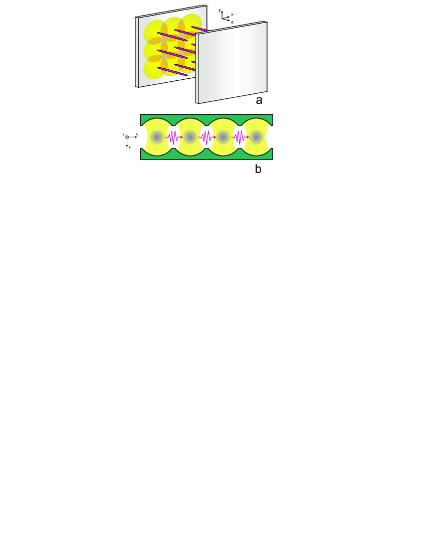
Figure 1: Schematic representation of the two models for polaritonic crystals: (a) trapped ensembles of ultracold atoms in a cavity interact with a quantised light field, whose distribution is represented by grey circles; (b) polaritonic crystal formed by an array of microcavities containing macroscopic ensembles of two-level atoms.

Model 2 considers a lattice of $M$ tunnelling-coupled microcavities in the $xy$ plane (Fig. 1b). Each cavity contains two-level atoms interacting with the electromagnetic field along the $z$ axis. The polaritonic crystals differ fundamentally from coupled-resonator optical waveguides (see, e.g., [6]) in that they offer the possibility of photon tunnelling in the $xy$ plane, normal to the main axis of the cavities.

It can be shown that, in the limit of so-called strong coupling between neighboring cells (cavities in model 2) containing atoms, the two models schematically illustrated in Fig. 1 give the same physical results. In this approximation, an atomic system can be described as a system of bosons (bosonic modes) that evolve only in time: its spatial degrees of freedom are frozen. This approximation is valid when the number of atoms $N$ in each cell is relatively small ($N\leq 10^{4}$) [14]. The height of the potential barrier between the cells of the optical lattice far exceeds the chemical potential of each atomic ensemble [16]. Otherwise, it is necessary to take into account the spatial configuration of the atomic system, which leads to the formation of spatially localised atomic structures [17].

Here, we restrict ourselves to the strong coupling approximation, completely neglecting interatomic interactions and taking the atomic ensembles in the cells to be an ideal gas. It will become clear from the analysis below that the polariton model for atom-photon coupling is then quite correct.

To be more specific, we consider model 1 of polaritonic crystal. The strong atom-photon coupling condition is thought to be fulfilled: the coupling parameter $\kappa$ in each cell of the lattice is substantially greater than the inverse of the coherence time, $\tau_{coh}$, of the atom–photon system:

$$\kappa\gg\frac{1}{\tau_{coh}}.$$ (1)

The total Hamiltonian of the system is

$$H=H_{at}+H_{int}+H_{ph},$$ (2)

where

$$H_{at}=\sum\limits_{j=a,b}\int{\Phi_{j}^{+}\left(-\frac{\hbar^{2}\Delta}{2M_{at}}+V_{ext}^{(j)}\right)\Phi_{j}d^{3}\vec{r}},\\$$ (3)

$$H_{ph}=\hbar\kappa\int{\left(\Psi^{+}\Phi_{a}^{+}\Phi_{b}+\Phi_{b}^{+}\Phi_{a}\Psi\right)d^{3}\vec{r}},\\$$ (4)

$$H_{int}=\int{\Psi^{+}\left(-\frac{\hbar^{2}\Delta_{\bot}}{2M_{ph}}+V_{ph}\right)\Psi d^{2}\vec{r}}.$$ (5)

Here, $H_{at}$ represents the ensemble of noninteracting two-level atoms in the trap; $H_{int}$ represents the atom photon interaction in the cavity in the rotating wave approximation; $H_{ph}$ represents the light field in the cavity in the paraxial approximation; $\Phi_{j}(\Phi_{j}^{+})$ are the boson annihilation (creation) operators for the levels $j=a$ and $b$; $M_{at}$ is the mass of a free atom; $\Delta$ is the Laplace operator; $V_{ext}^{(j)}$ is the total atom trapping potential, which comprises the harmonic potential of the magneto-optical trap and the optical lattice potential along the $x$ and $y$ axes [18]; $\Psi(\Psi^{+})$ is the annihilation (creation) operator for a field propagating along the $z$ axis of the cavity, $M_{ph}=\hbar k_{z}/c$ is the photon effective mass in the cavity; $k_{z}$ is the $z$-axis projection of the optical field wave vector; $V_{ph}$ is the photon trapping potential in the atom-photon coupling region, which can be created by special gradient-index lenses or fibres [8]; and $\Delta_{\bot}=\partial^{2}/\partial x^{2}+\partial^{2}/\partial y^{2}$.

For an array of $M$ cells in an optical lattice, the $\Phi_{j}$ and $\Psi$ operators can be represented in the form

$$\Phi_{a}=\sum\limits_{m=1}^{M}a_{m}(t)\varphi_{m}^{a}(\vec{r}),\\$$ (6)

$$\Phi_{b}=\sum\limits_{m=1}^{M}b_{m}(t)\varphi_{m}^{b}(\vec{r}),\\$$ (7)

$$\Psi=\sum\limits_{m=1}^{M}\psi_{m}(t)\xi_{m}(\vec{r}),\\$$ (8)

where $\varphi_{m}^{a,b}(\vec{r})$ and $\xi_{m}(\vec{r})$ are the real-valued Wannier functions describing the spatial distributions of the atoms and field, respectively, in the $m$th cell $(m=1,...,M)$. In the limit of strong coupling between neighbouring cells (so-called tight-binding approximation), the $\varphi_{m}^{a,b}$ functions satisfy the relations [16, 17]

$$\int|\varphi_{m}^{a,b}|^{2}d^{3}\vec{r}=1,\quad\int\varphi_{m}^{a,b}\varphi_{m+1}^{a,b}d^{3}\vec{r}\simeq 0.$$ (9)

Analogous relations are valid for the $\xi_{m}(\vec{r})$ functions. The $a_{m}(t)$ and $b_{m}(t)$ operators characterise the dynamic behaviour of the two components (two modes) of the atomic ensemble at the lower and upper levels, respectively, and the $\psi_{m}(t)$ operator describes the time evolution of the cavity field in the $m$th cell of the lattice.

Substituting (6)-(8) into (3)-(5) we obtain

$$H_{at}=\hbar\sum\limits_{m=1}^{M}[\omega^{a}_{mat}a^{+}_{m}a_{m}+\omega^{b}_{mat}b^{+}_{m}b_{m}-\frac{\beta_{a}}{2}(a_{m}^{+}a_{m-1}+a_{m}^{+}a_{m+1}+h.c.)-\frac{\beta_{b}}{2}(b_{m}^{+}b_{m-1}+h.c.)],\\$$ (10)

$$H_{int}=\hbar\sum\limits_{m=1}^{M}g_{m}(\psi_{m}^{+}a_{m}^{+}b_{m}+b_{m}^{+}a_{m}\psi_{m}),\\$$ (11)

$$H_{ph}=\hbar\sum\limits_{m=1}^{M}[\omega_{mph}\psi_{m}^{+}\psi_{m}-\frac{\alpha}{2}(\psi_{m}^{+}\psi_{m-1}+\psi_{m}^{+}\psi_{m+1}+h.c.)],$$ (12)

where the coupling coefficients $\beta_{a,b}$ and $\alpha$ characterise atom (photon) tunnelling between neighbouring cells and are determined by the overlap integrals of the $\varphi_{m}^{a,b}(\vec{r})$ and $\xi_{m}(\vec{r})$ functions with their derivatives, respectively. The quantities $\omega_{mat}^{a,b}$ and $\omega_{mph}$ are defined in an analogous way [16, 17]. We take all the atom-photon coupling coefficients to be the same in all the cells: $g=g_{1}=g_{2}=...=g_{M}$.

Let us turn to the momentum ($\vec{k}$-space) representation. Given that polaritonic crystals have a periodic structure, the $\psi_{m}$, $a_{m}$ and $b_{m}$ operators can be represented in the form

$$a_{m}=\frac{1}{\sqrt{M}}\sum\limits_{\vec{k}}a_{\vec{k}}exp(i\vec{k}\vec{n}),\quad b_{m}=\frac{1}{\sqrt{M}}\sum\limits_{\vec{k}}b_{\vec{k}}exp(i\vec{k}\vec{n}),\quad\psi_{m}=\frac{1}{\sqrt{M}}\sum\limits_{\vec{k}}\psi_{\vec{k}}exp(i\vec{k}\vec{n}),$$ (13)

where $\vec{n}$ is a lattice vector.

For simplicity, we examine a 1D polaritonic crystal structure below, for which $\vec{k}\vec{n}=mk_{x}l$, where $k_{x}$ is the $x$- axis projection of the optical field wave vector and $l$ is the lattice constant. Substituting (13) into (10)-(12), we obtain the $\vec{k}$-space Hamiltonian

$$H=\hbar\sum\limits_{\vec{k}}\left(\omega_{ph}(k)\psi_{\vec{k}}^{+}\psi_{\vec{k}}+\frac{1}{2}\omega_{at}(k)\left(b_{\vec{k}}^{+}b_{\vec{k}}-a_{\vec{k}}^{+}a_{\vec{k}}\right)+\frac{g}{\sqrt{M}}\sum\limits_{\vec{q}}\left(\psi_{\vec{k}}^{+}a_{\vec{q}}^{+}b_{\vec{k}+\vec{q}}+b_{\vec{k}+\vec{q}}^{+}a_{\vec{q}}\psi_{\vec{k}}\right)\right).$$ (14)

Here $\omega_{ph}(k)$ and $\omega_{at}(k)$ determine the dispersion relations for the photonic and atomic systems of the polaritonic crystal, respectively, and are given by

$$\omega_{ph}(k)=\omega_{mph}-2\alpha cos(kl),\quad\omega_{at}(k)=\omega_{mat}^{b}-\omega_{mat}^{a}-2\beta cos(kl),$$ (15)

where $\beta=\beta_{b}-\beta_{a}$ is the effective coupling coefficient of the atomic lattice.

III Quantum degeneracy of a 1D polariton gas

In the strong coupling regime, expression (14) is a many particle Hamiltonian in the momentum representation, which describes a 1D periodic structure and can be analysed in terms of dark- and bright-state polaritons. We will consider it in the low atomic excitation density limit, where all the atoms predominantly occupy the lower level $|a\rangle$ [11]. The boson annihilation ($\phi_{\vec{k}}$) and creation ($\phi_{\vec{k}}^{+}$) operators for collective excitations in a two-level atomic system can then be defined in the $\vec{k}$-space representation:

$$\phi_{\vec{k}}=\sum_{\vec{q}}\frac{a_{\vec{q}}^{+}b_{\vec{k}+\vec{q}}}{\sqrt{MN}},\qquad\phi_{\vec{k}}^{+}=\sum_{\vec{q}}\frac{b_{\vec{k}+\vec{q}}^{+}a_{\vec{q}}}{\sqrt{MN}}.$$ (16)

Using (16), Hamiltonian (14) of the system can be represented in a more convenient form:

$$H=\hbar\sum\limits_{\vec{k}}\left(\omega_{ph}(k)\psi_{\vec{k}}^{+}\psi_{\vec{k}}+\omega_{at}(k)\phi_{\vec{k}}^{+}\phi_{\vec{k}}+g\left(\psi_{\vec{k}}^{+}\phi_{\vec{k}}+\phi_{\vec{k}}^{+}\psi_{\vec{k}}\right)\right),$$ (17)

where we denote again g instead of $g\sqrt{N}$ . Hamiltonian (17) can be diagonalised using the Bogoliubov transformations

$$\Xi_{1,\vec{k}}=\mu_{1}\psi_{\vec{k}}-\mu_{2}\phi_{\vec{k}},\qquad\Xi_{2,\vec{k}}=\mu_{1}\phi_{\vec{k}}+\mu_{2}\psi_{\vec{k}},$$ (18)

where

$$\mu_{1,2}^{2}=\frac{1}{2}\left[1\mp\frac{\delta\omega}{(\delta\omega^{2}+4g^{2})^{1/2}}\right]$$ (19)

are Hopfield coefficients satisfying the normalisation condition $\mu_{1}^{2}+\mu_{2}^{2}=1$; $\delta\omega=\omega_{at}(k)-\omega_{ph}(k)=\Delta-2(\beta-\alpha)\times\cos(kl)$ is the frequency detuning, dependent on quasimomentum $k$; and $\Delta\equiv\omega_{mat}^{b}-\omega_{mat}^{a}-\omega_{mph}$ is the detuning at $kl=\pi/2+\pi p$ with $p=0,1,...$.

The $\Xi_{1\vec{k}}$ and $\Xi_{2\vec{k}}$ operators in (18) represent two types of elementary excitations in an atomic system upper and low branch polaritons, with characteristic frequencies $\Omega_{1,2}(k)$, that determine the dispersion relations and band structure of PolC. The frequencies are given by the expression

$$\Omega_{1,2}(k)=\frac{1}{2}\left[\omega_{at}(k)+\omega_{ph}(k)\pm\sqrt{\delta\omega^{2}+4g^{2}}\right],$$ (20)

Using (20), one can find the mass of the upper (subscript 1) and low (subscript 2) branch polaritons:

$$m_{1,2}=\frac{2m_{at}m_{ph}\sqrt{\tilde{\Delta}^{2}+4g^{2}}}{(m_{at}+m_{ph})\sqrt{\tilde{\Delta}^{2}+4g^{2}}\mp(m_{at}-m_{ph})\tilde{\Delta}}$$ (21)

where $\tilde{\Delta}=\Delta-2(\beta-\alpha)$ is an effective detuning, which includes the characteristic frequencies $\alpha$ and $\beta$, $m_{at}=\hbar/(2\beta l^{2})$ and $m_{ph}=\hbar/(2\alpha l^{2})$ are the effective masses of the atoms and photons in the lattice, respectively.

Figure 2 shows the upper and low branch polariton dispersion, $\Omega_{1,2}(k)$, in the first Brillouin zone. The band gap is determined by the Rabi splitting: $(\delta\omega^{2}+4g^{2})^{1/2}$. In the center of the zone (near $k=0$), both dispersion branches are parabolic. At resonance ($\delta\omega=0$), the splitting is governed by the atom–photon coupling coefficient $2g$ (see also the inset in Fig. 2).

The minimum at $k=0$ in the lower polariton branch in Fig. 2 is of fundamental importance. At small magnitudes of the quasi-momentum, $kl\ll 1$, we have from (20)

$$\Omega_{2}(k)\approx\frac{\hbar k^{2}}{2m_{2}},$$ (22)

which corresponds to the dispersion law of free particles (polaritons) at the minimum in $\Omega_{2}(k)$ in Fig. 2. The statistical properties of the polariton gas are then governed by its dimensionality (see, e.g., [19]). In particular, in the case of resonance coupling the low branch polariton mass can be found from (21):

$$m_{2}=\frac{2m_{ph}}{1+m_{ph}/m_{at}}.$$ (23)

Figure 2: Polariton dispersion branches $\Omega_{1}$ (dashed curve) and $\Omega_{2}$ (solid curve) as functions of reduced quasi-momentum (Bloch vector) in the first Brillouin zone. The characteristic frequency of the atomic transition is $(\omega_{mat}^{b}-\omega_{mat}^{a})/2\pi=500THz$, $\Delta=0$, the atom–photon coupling frequency is $g(2\pi)^{-1}=2GHz$, the photon (atom) effective mass in the lattice is $m_{ph}=5\times 10^{-36}kg$ ($m_{at}=38.5\times 10^{-27}kg$), and the lattice constant is $l=2.24\mu m$. The inset shows the frequency range of Rabi splitting.

For $m_{ph}/m_{at}\ll 1$ ($\alpha\gg\beta$), the polariton mass is sufficiently small. For example, in the case of interaction of two-level sodium atoms with an electromagnetic field in a cavity at a level separation wavelength of 589 nm, the photon effective mass in the cavity is $m_{ph}\simeq 0.5\times 10^{-35}kg$ [12]. The polariton mass estimated by Eq. (23) is then $m_{2}\simeq 10^{-35}kg$. Therefore, the quantum degeneracy temperature of a 1D polariton gas, $T_{d}=2\pi\hbar^{2}n_{1}^{2}/(m_{2}k_{B})$, may be rather high ($\sim 300K$ at a polariton density $n_{1}\simeq 10^{4}cm^{-1}$). It should, however, be kept in mind that the spatially periodic structure of the polaritonic crystal in Fig. 1 has a long coherence time only at sufficiently low temperatures, where a relatively large number of atoms can be trapped. The polariton gas can be considered a highly degenerate quantum system, meeting the condition $n_{1}\Lambda_{T}\gg 1$, where $\Lambda_{T}=[2\pi\hbar^{2}/(m_{2}k_{B}T)]^{1/2}$ is the de Broglie wavelength. In this limit, the formation of coherent polaritons in a polaritonic crystal is of interest for spatially distributed recording and storage of quantum optical information [20, 21].

IV Group velocity of polaritons

Consider the group velocities $v_{1,2}=\partial\Omega_{1,2}(k)/\partial k$ of polaritons in a lattice. From (20) we obtain

$$v_{1,2}=\frac{\hbar\sin{(kl)}}{2lm_{ph}}\left[1+\frac{m_{ph}}{m_{at}}\mp\left(1-\frac{m_{ph}}{m_{at}}\right)\frac{\delta\omega}{\sqrt{\delta\omega^{2}+4g^{2}}}\right]$$ (24)

It follows from (24) that the group velocities $v_{1,2}$ of polaritons are low at small $\vec{k}$. In particular, in the $kl\ll 1$ limit the low branch polariton has a linear $v_{2}(k):v_{2}\simeq\hbar k/m_{2}$. At the same time, $v_{1,2}=0$ at the boundaries of the Brillouin zone, i.e., at $kl=p\pi,p=0,\pm 1,...$. In this case, the structure of the polaritonic crystal allows polaritons to be fully localised within this zone.

The ability to reduce the group velocity of polaritons can be used to observe ‘slow’ light, which is of high current interest for quantum optical information recording and storage. In our case, the group velocity of the optical field can be varied by changing the atom-field detuning $\Delta$ (or $\tilde{\Delta}$).

The possibility of controlling low branch polaritons with small magnitudes of the quasi-momentum, k, is exemplified in Fig. 3. Control is performed near the bottom of the well in Fig. 2, where the parabolic dispersion law (22) is valid. In this limit, polaritons can be assigned a wave function, $\Psi(x,t)$, which carries quantum information and satisfies free particle Schrödinger equation:

$$\left(i\hbar\frac{\partial}{\partial t}+\frac{\hbar^{2}}{2m_{2}}\frac{\partial^{2}}{\partial x^{2}}\right)\Psi(x,t)=0.$$ (25)

The solution to Eq. (25) is well known in quantum physics (see, e.g., [13, 22]). Polaritons are a coherent wave packet that broadens with time and propagates through the polaritonic crystal (Fig. 1b). The characteristic wave packet broadening time, $\tau_{b}=m_{2}f^{2}/\hbar$, depends on both the polariton mass, $m_{2}$, and the $x$-axis width of the packet, $f$, at the initial instant, that is, on the incident beam diameter.

Quantum optical information recording and storage using PolC is expected to have a three-step physical algorithm based on the ability to control the group velocity of a polariton wave packet in the medium by varying the $\tilde{\Delta}$ detuning (Fig. 3a).

For quantum information to be recorded in step I, the $\tilde{\Delta}$ detuning must fulfil the condition $\tilde{\Delta}\gg 2|g|$. The corresponding time interval in Fig. 3a is $0\leq\tau\leq 0.25$. The low branch polariton is here photon-like, i.e., $\Xi_{2\vec{k}}\simeq-\psi_{\vec{k}}$ ($\mu_{1}\simeq 0,\mu_{2}\simeq-1$), and its effective mass $m_{2}\simeq m_{ph}$ [see Eqs. (18), (19) and (21)]. The wave packet then propagates at a velocity given by

$$v_{2}=\frac{\hbar k}{m_{ph}}=2\alpha l^{2}k,$$ (26)

and displaces along the $x$ axis from the point $x=0$ to $x=v_{2}t$ (Fig. 3b). For example, at a quasi-momentum $k=10^{5}m^{-1}$ the estimated polariton group velocity is $v_{2}=2\times 10^{6}m/s$.

To map the optical information to coherent excitations of the medium in step II, the detuning should be made negative: $\tilde{\Delta}\ll-2|g|$. In this limit, the low branch polariton becomes atom-like, so that $\Xi_{2\vec{k}}\simeq\phi_{\vec{k}}$ ($\mu_{1}\simeq 1,\mu_{2}\simeq 0$) (Fig. 3). At $m_{ph}/m_{at}=\beta/\alpha\ll g^{2}/\Delta^{2}$, its group velocity is [7]

$$v_{2}=\frac{\hbar kg^{2}}{m_{ph}\tilde{\Delta}^{2}}=\frac{2\alpha l^{2}kg^{2}}{\tilde{\Delta}^{2}}.$$ (27)

When the more stringent condition $\frac{g^{2}}{\tilde{\Delta^{2}}}\ll\frac{m_{ph}}{m_{at}}\ll 1$ is fulfilled, the low-branch polariton group velocity is

$$v_{2}=\frac{\hbar k}{m_{at}}=2\beta l^{2}k,$$ (28)

which corresponds to the velocity of the atoms in the lattice. In particular, for sodium atoms with an effective mass $m_{at}=38.5\times 10^{-27}kg$ the group velocity of such polaritons at the above wave vector is $v_{2}=2.6\times 10^{-4}m/s$ [21].

In fact, Eq. (28) determines the lower limit of the velocity of an optical wave packet in the structure of a polaritonic crystal at a given quasi-momentum. In this limit, all the information carried by a light beam is recorded and stored via atomic excitations. At an incident beam diameter $f\simeq 10^{-4}m$, the estimated characteristic broadening time is $\tau_{b}=m_{at}f^{2}/\hbar\approx 3.7s$. This time scale (the interval $0.25\leq\tau\leq 0.75$ in Fig. 3a) determines the longest information storage time in a quantum gas of two-level sodium atoms. More precisely, a necessary condition for such information recording is $t_{stor}\ll\tau_{b}$ (where $t_{stor}$ is the information storage time in the atomic system), which implies that the wave packet retains its shape during the whole period of quantum state storage.

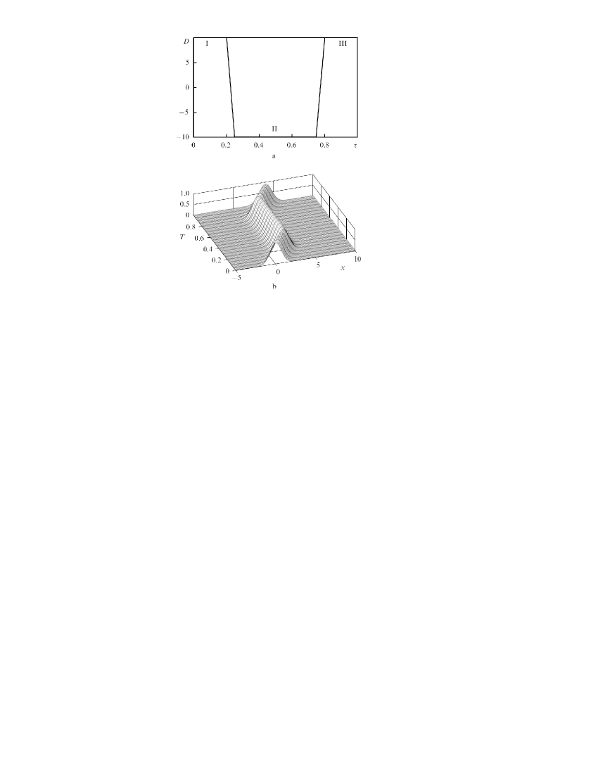
Figure 3: Propagation of a 1D polariton wave packet through a polaritonic crystal: (a) $D=\tilde{\Delta}/(2|g|)$ as a function of normalised time $\tau=\hbar t/(m_{ph}f^{2})$ and (b) wave packet envelope (probability density) $S\equiv|\Psi(x,t)|^{2}/|\Psi(0,0)|^{2}$ as a function of $\tau$ and normalised coordinate $X=x/f$ at $k_{x}f=10$; optical information (I) recording, (II) storage and (III) reading (retrieving) steps.

To restore (read) optical information at the output of the medium after time $t_{stor}$ (step III), the polaritons must be again made photon-like by switching the $\tilde{\Delta}$ detuning in the reverse direction. In Fig. 3a, the characteristic reverse switching time of the wave packet, $t_{retr}$, is determined by the time interval $0.75\leq\tau\leq 0.8$. At the output ($\tau=1$), we again have an optical wave packet, which is displaced along the $x$ axis in a plane normal to the cavity axis.

In this work, we do not assess the quality (fidelity) of information storage. Alodjants et al. [13] estimated the information storage fidelity taking into account only changes in wave packet shape, but this is generally insufficient. It is, in addition, necessary to analyse transformations of the quantum state of the optical field with consideration for the structure of the polaritonic crystal and its decoherence (see, e.g., [23]). Analysis of this problem is of interest on its own and is beyond the scope of this paper. We note only that, under real experimental conditions, the information recording, storage and reading time is limited by the decoherence time of the polaritonic crystal. It is therefore quite reasonable to use a condensate of atoms that have a sufficiently long macroscopic coherence time–tens of microseconds according to experimental data [24].

V Conclusions

We examined a lattice model of coherent polaritons in a spatially periodic structure a polaritonic crystal formed by a lattice of ensembles of two-level atoms effectively interacting with quantised electromagnetic field in a cavity (or in a 2D lattice of cavities) in the strong coupling regime. Our results demonstrate that the structure of PolC allows the low branch polariton to be fully localised, which can be used, first, to achieve quantum degeneracy of the polariton gas and, second, to substantially slow down group velocity of light pulses in such media. The coherence properties of an ensemble of polaritons were discussed from the viewpoint of spatially distributed quantum recording, storage and retrieving of information related to a propagating optical wave packet.

References

- (1) Akhmanov S.A., Vorontsov M.A. (Eds) Novye fizicheskie printsipy opticheskoi obrabotki informatsii (Novel Physical Principles of Optical Information Processing) (Moscow: Nauka, 1990).
- (2) Bloch I. J. Phys. B: At. Mol. Opt. Phys., 38, S629 (2005).
- (3) Brennecke F., Donner T., Ritter S., Bourdel T., Kohl M., Esslinger T. Nature, 450, 268 (2007).
- (4) Hartmann M.J., Brandao F., Plenio M.B. Nature, 2, 849 (2006).
- (5) Aoki T., Dayan B., Wilcut E., Bowen W.P., Parkins A.S., Kippenberg T.Y., Vahala K.Y., Kimble H.J. Nature, 443, 671 (2006).
- (6) Zhou L., Lu J., Sun C.P. Phys. Rev. A, 76, 012313 (2007).
- (7) Yanik M.F., Fan S. Phys. Rev. Lett., 92, 083901 (2004).
- (8) Averchenko V.A., Alodjants A.P., Arakelian S.M., Bagaev S.N., Vinogradov E.A., Egorov V.S., Stolyarov A.I., Chekhonin I.A. Kvantovaya Elektron., 36, 532 (2006) [ Quantum Electron., 36, 532 (2006)].
- (9) Kavokin A., Malpuech G., Laussy F.P. Phys. Lett. A, 306, 187 (2003).
- (10) Kasprzak J., Richard M., Kundermann S., Baas A., et al. Nature, 443, 409 (2006).
- (11) Alodjants A.P., Arakelian S.M., Bagayev S.N., Egorov V.S., Leksin A.Yu. Appl. Phys. B, 89, 81 (2007).
- (12) Lai C.W., Kim N.Y., Utsunomiya S., Roumpos G., Deng H., Fraser M.D., Byrnes T., Recher P., Kumada N., Fujisawa T., Yamamoto Y. Nature, 450, 529 (2007).
- (13) Alodjants A.P., Arakelian S.M., Leksin A.Yu. Laser Phys., 17, 1432 (2007).
- (14) Anglin J.R., Vardi A. Phys. Rev. A, 64, 013605 (2001).
- (15) Cirac J.I., Lewenstein M., Molmer K., Zoller P. Phys. Rev. A, 57, 1208 (1998).
- (16) Smerzi A., Trombettoni A., Kevrekidis P.G., Bishop A.R. Phys. Rev. Lett., 89, 170402 (2002).
- (17) Brazhny V.V., Konotop V.V. Mod. Phys. Lett. B, 18, 627 (2004); Alfimov G.L., Kevrekidis P.G., Konotop V.V., Salerno M. Phys. Rev. E, 66, 046608 (2002).
- (18) Kramer M., Menotti C., Pitaevskii L., Stringari S. Eur. Phys. J. D, 27, 247 (2003).
- (19) Petrov D.S., Gangardt G.M., Shlyapnikov G.V. J. Phys. IV France, 116, 7 (2004).
- (20) Mishina O.S., Kupriyanov D.V., Müller J.H., Polzik E.S. Phys. Rev. A, 75, 042326 (2007).
- (21) Fleischauer M., Lukin M.D. Phys. Rev. A, 65, 022314 (2002).
- (22) Karlov N.V., Kirichenko N.A. Nachal’nye glavy kvantovoi mekhaniki (The Initial Chapters of Quantum Mechanics) (Moscow: Fizmatlit, 2004).
- (23) He Q.Y., Reid M.D., Giacobino E., Cviklinski J., Drummond P.D. E-print arXiv:0808.2010v1 [quant-ph] 14 Aug 2008.
- (24) Liu C., Dutton Z., Behroozi C.H., Hau L.V. Nature, 409, 490 (2001).