A nonequilibrium theory for transient transport dynamics in nanostructures
via the Feynman-Vernon influence functional approach

Abstract

In this paper, we develop a nonequilibrium theory for transient electron transport dynamics in nanostructures based on the Feynman-Vernon influence functional approach. We extend our previous work on the exact master equation describing the non-Markovian electron dynamics in the double dot [Phys. Rev. B78, 235311 (2008)] to the nanostructures in which the energy levels of the central region, the couplings to the leads and the external biases applied to leads are all time-dependent. We then derive nonperturbatively the exact transient current in terms of the reduced density matrix within the same framework. This provides an exact non-linear response theory for quantum transport processes with back-reaction effect from the contacts, including the non-Markovian quantum relaxation and dephasing, being fully taken into account. The nonequilibrium steady-state transport theory based on the Schwinger-Keldysh nonequilibrium Green function technique can be recovered as a long time limit. For a simple application, we present the analytical and numerical results of transient dynamics for a resonant tunneling nanoscale device with a Lorentzian-type spectral density and ac bias voltages, where the non-Markovian memory structure and non-linear response to the time-dependent bias voltages in transport processes are demonstrated.

I introduction

The investigation of quantum coherence dynamics far away from equilibrium in nanoscale electronic devices has been attracting much attentions in the past decade due to various applications in nanotechnology and quantum information processing. Experimentally it became possible not only to directly manufacture structures but also to investigate their nonequilibrium quantum coherence properties under well controlled parameters.Gol98156 ; Cro98540 ; Lu03422 ; Hay03226084 ; Pet051280 ; Fuj06759 ; Han071217 Theoretically, tremendous studies have been done focusing on the time-independent steady-state to analyze the nonequilibrium transport properties. However, an increasing number of work employing various theoretical techniques (see Refs. [Win938487, ; Jau945528, ; Bru941076, ; Kon9616820, ; Sun004754, ; Zhu03224413, ; Li05205304, ; And05196801, ; Lee06085325, ; Mac06085324, ; Jin08234703, ; Wei08195316, ; Sch08235110, ; Tu08235311, ; Zed09045309, ; Zhe09164708, ; Hau98, ]) has recently occurred addressing the time-dependent electron dynamics far away from the equilibrium. In fact, for practical applications, a full understanding of nonequilibrium dynamics under external field controls, i.e., the time evolution of electrons in nanoelectronics devices from some initial preparation toward any specifically designed state within an extremely short time, has been receiving more and more attentions.

The prototypical nanostructure concerned in this paper is made by a gate-defined region on a semiconductor containing a few of discrete electronic states. Electrodes are implanted around this central region to control the electrons across it. Also gates are deposited to adjust the electronic states within the central area as well as their couplings to the surrounding electrodes. Most of the theoretical developments to nanoelectronics devices have been focusing on the understanding and prediction of transport dynamics in these devices. However, as a quantum device, in particular for quantum information processing,Hay03226084 ; Pet051280 ; Fuj06759 ; Han071217 the big challenge is to understand and predict not only how fast or slow a nanoelectronic device can turn on or off a current, but also how reliable and efficient the device can manipulate quantum coherence of the electron states through external bias and gate voltage controls. This requires a nonequilibrium quantum device theory to analyze the time-dependent quantum transport intimately entangling with quantum coherence of electrons inside the device. It is the purpose of this paper to attempt to establish a nonequilibrium theory of transient dynamics for electron quantum states accompanied with electron quantum transport in a nanoelectronic device that can be feedbackly controlled through the non-linear response to the external time-dependent bias and gate voltage pulses.

Physically the nanostructure we are going to study is typically an open quantum system in the sense that its central region has exchanges of particles, energy and information with its surroundings. From an open quantum system point of view, the nonequilibrium electron dynamics is completely described by the master equation through the physical observable $\langle O(t)\rangle={\rm tr}[O\rho(t)]$, where $\rho(t)$ is the reduced density matrix of the central system that can fully depict the dynamics of electron quantum states and is determined by the master equation. The transient electron transport should be in principle solved from the reduced density matrix as well. However, it has been struggled for many years without a very satisfactory answer in finding the exact master equation for an arbitrary open quantum system.Hua87 Most of the master equations used in the literature are obtained using semiclassical approximation or perturbation truncation, such as the semiclassical Boltzmann equationCer75 ; Smi89 or master equations under the Born-Markov approximation.Car93 ; Bre02 However, for the nanostrucutres with the extremely short length scales ($\sim$1 nm) and extremely fast time scales ($\sim$1 fs), the semiclassical Boltzmann equation or the master equation under the Born-Markov approximation are most unlikely applicable.Hau98

Literarily, there are two fundamental but equivalent methods in dealing with modern nonequilibrium physics. They are the Schwinger-Keldysh nonequilibrium Green function techniqueSch61407 ; Kad62 ; Kel651018 and the Feynman-Vernon influence functional approach.Fey63118 In the practical applications, both methods have their own advantages. The Schwinger-Keldysh nonequilibrium Green function technique is a standard method for systematic perturbation calculations to various nonequilibrium physical processes in many-body systems.Cho851 ; Ram86323 As it is evidenced the nonequilibrium Green function technique provides an extremely powerful tool in the study of the steady-state transport properties in nanostructures.Mei913048 ; Mei922512 ; Dat95 ; Hau98 In the steady-state limit where the initial state of the nanostructure is irrelevant, the transport current can be expressed in terms of the nonequilibrium Green functions in the frequency domain which largely simplifies the transport problem. Without the time-dependence, the physics of the nonequilibrium transport is essentially determined by the density of states (the difference between the retarded and the advanced Green functions). The nonequilibrium Green function technique has been used to successfully describe a variety of new phenomena, such as Kondo effect, Fano resonance and Coulomb blockade effects in quantum dots. The extension of the nonequilibrium Green function techniques to the time-dependent transport phenomena in nanostructures has also been developedWin938487 ; Jau945528 ; Sun004754 ; Zhu03224413 ; Hau98 where the time-dependent nonequilibrium Green functions must be maintained. Except for the wide band limit (WBL),Jau945528 ; Hau98 the relevant Green function calculations become rather complicated in order to taking into account the different initial quantum state effect and the non-Markovian memory structure.Mac06085324 ; Sch08235110

On the other hand, the Feynman-Vernon influence functional approachFey63118 are mainly used to study dissipation dynamics in quantum tunneling problemsLeg871 and decoherence problems in quantum measurement theory.Zuk03715 It is very powerful to derive nonperturbatively the master equation for the reduced density matrix of an open system by integrating out completely the environmental degrees of freedom through the path integral approach, where the non-Markovian memory structure is manifested explicitly. In the early applications of the influence functional approach, the master equation was derived for some particular class of Ohmic (white-noise) environment for the quantum Brownian motion (QBM) modeled as a central harmonic oscillator linearly coupled to a set of harmonic oscillators simulating the thermal bath.Cal83587 ; Haa852462 The exact master equation for the QBM with a general spectral density (color-noise environments) at arbitrary temperature that can fully address the non-Markovian dynamics was the Hu-Paz-Zhang master equation.Hu922843 Applications of the QBM exact master equation cover various topics, such as quantum decoherence, quantum-to-classical transition, quantum measurement theory, and quantum gravity and quantum cosmology, etc.Wei99 ; Bre02 ; Hu08 Very recently, such an exact master equation is further extended to the systems of two entangled bosonic fields An07042127 ; Cho08011112 ; An090317 for the study of non-Markovian entanglement dynamics.Yu04140404 Nevertheless, using the influence functional approach to obtain the exact master equation has been largely focused on the bosonic (thermal) environments in the past half century.

Meanwhile, using master equation to study quantum electron transport has also been attracting much attentions recently. With the nonequilibrium Green function technique, the master equation can be formally obtained in terms of real-time diagrammatic expansion up to all the orders,Sch9418436 ; Kon961715 ; Kon9616820 ; Lee08224106 although practically most of the master equation approach used in quantum transport by far only take the perturbative theory up to the second order.Leh02228305 ; Li05205304 ; Ped05195330 ; Wel06044712 ; Har06235309 ; Cui06449 On the other hand, with the help of the influence functional approach, an alternative formalism for the master equation for studying quantum transport and electron dissipative dynamics has recently been developed in term of the hierarchical expansion.Jin08234703 This new master equation approach provides a very efficient tool for the numerical study of the quantum transport properties, including the accurate evaluations of the Coulomb blockage and Kondo transition dynamics.Zhe08093016 ; Zhe09164708

In this paper, we shall develop a nonequilibrium theory to describe nonperturbatively the transient electron transport dynamics intimately entangling with the electron quantum decoherence in nanostructures. By extending the influence functional approach to the fermionic reservoirs, we have recently derived an exact master equation for a large class of nanostructures.Tu08235311 This exact master equation is capable for the study of the full non-Markovian decoherence dynamics of electrons in nanoelectronics devices. In the present work, we shall extend the previous work to the nanostructures in which the energy levels of the central region, the couplings to the leads and the external biases applied to leads are all time-dependent. We then derive the exact transient current in terms of the reduced density matrix within the same framework. The resulting transient current provides an exact non-linear response theory that can be used to investigate the transient quantum transport processes accompanied explicitly with the non-Markovian quantum relaxation and dephasing dynamics. The nonequilibrium steady-state transport theory based on the nonequilibrium Green function technique that is widely used in the literature can be recovered as a long time limit from the present theory.

The remainder of this paper is organized as follows. In Sec. II, we outline the derivation of the exact master equation we obtained recently,Tu08235311 with the extension to the time-dependent Hamiltonian for a general nanostructure. In Sec. III, we derive in detail the exact transient current in terms of the reduced density operator based on the Feynman-Vernon influence functional approach. The resulting transient current $I_{\alpha}(t)$ through the lead $\alpha$ is given by the general formula, Eq. (19), or equivalently Eq. (30), which is valid for arbitrary bias and gate voltage pulses with arbitrary energy-dependent couplings between the central system and the leads. The relation between the reduced density matrix and the transient current is established through the master equation, see Eq. (23) where the superoperators ${\cal L}^{+}_{\alpha}(t)$ and ${\cal L}^{-}_{\alpha}(t)$ given explicitly by Eq. (20) and (22) encompass all the back-reaction effects associated with the non-Markovian dynamics of the central system interacting with the lead $\alpha$. The steady-state current formula based on the nonequilibrium Green function technique can be recovered as a long time limit, see Sec. III.E. Applications to transient dynamics with Lorentzian-type spectral density and various time-dependent ac bias voltages are demonstrated in Sec. IV. The summary and prospective are given in Sec. V. In Appendix, a close connection between the Feynman-Vernon influence functional approach and the Schwinger-Keldysh nonequilibrium Green function technique for quantum transport theory is established.

II Exact master equation for nanoscale electronic devices

In this section, we shall outline the exact master equation derived recently by two of us for nanoscale electronic devices Tu08235311 with the extension to the time-dependent energy levels and couplings. We shall only list the necessary formula that we will use later for the derivation of the transient current. For more detailed derivation, please refer to Ref. [Tu08235311, ]. We begin with the Hamiltonian of a prototypical mesoscopic system for electron transport,

$$H(t)= \sum_{ij}\epsilon_{ij}(t)a^{\dagger}_{i}a_{j}+\sum_{\alpha k}\epsilon_{\alpha k}(t)c^{\dagger}_{\alpha k}c_{\alpha k}$$

$$+\sum_{i\alpha k}[V_{i\alpha k}(t)a^{\dagger}_{i}c_{\alpha k}+V^{*}_{i\alpha k}(t)c^{\dagger}_{\alpha k}a_{i}].$$ (1)

Here the first summation is the electron Hamiltonian $H_{S}$ for the central system where the electron-electron interaction is not considered. But as we have shown we can properly and explicitly exclude the doubly occupied states and the resulting master equation can be applied to the strong Coulomb repulsion (i.e. Coulomb blockage) regime.Tu08235311 The second summation is the Hamiltonian $\sum_{\alpha}H_{\alpha}$ describing the noninteracting electron leads (the source and drain electrodes, $\cdots$) labeled by the index $\alpha~{}(=L,R,\cdots$). The last term is the electron tunneling Hamiltonian $H_{T}$ between the leads and the central system. Since we will focus on the transient dynamics of quantum transport in this paper, the bias voltages $V_{\alpha}$ applied to leads are considered to be time-dependent. Thus the single electron energy levels in the leads is changed as $\epsilon_{\alpha k}\rightarrow\epsilon_{\alpha k}(t)=\epsilon_{\alpha k}+eV_{\alpha}(t)$. Meanwhile, the energy levels $\epsilon_{ij}$ of the central system and the couplings $V_{i\alpha k}$ between the central system and the leads are controllable through the gate voltages and external fields so that they can be, in general, also time-dependent: $\epsilon_{ij}\rightarrow\epsilon_{ij}(t)=\epsilon_{ij}+\Delta_{ij}(t),V_{i\alpha k}\rightarrow V_{i\alpha k}(t)$. Throughout this work, we set $\hbar=1$, except for the transient current where we will put $\hbar$ back from its definition.

The master equation for the nonequilibrium electron dynamics of the central system is derived based on the Feynman-Vernon influence functional approach.Fey63118 As it is well known,Hua87 the nonequilibrium electron dynamics of an open system is completely determined by the so-called reduced density matrix. The reduced density matrix is defined from the density matrix of the total system (the central system plus the leads, and the leads are treated as the reservoirs to the central system) by tracing over entirely the environmental degrees of freedom: $\rho(t)\equiv{\rm tr}_{\mbox{\tiny R}}\rho_{\rm tot}(t)$, where the total density matrix is formally given by $\rho_{\rm tot}(t)=U(t,t_{0})\rho_{\rm tot}(t_{0})U^{\dagger}(t,t_{0})$ with the evolution operation $U(t,t_{0})=T\exp\{-i\int^{t}_{t_{0}}H(\tau)d\tau\}$, and $T$ is the time-ordering operator. As usual, we assume that the central system is uncorrelated with the reservoirs before the tunneling couplings are turned on:Leg871 $\rho_{\rm tot}(t_{0})=\rho(t_{0})\otimes\rho_{R}(t_{0})$, and the reservoirs are initially in the equilibrium state: $\rho_{R}(t_{0})={1\over Z}e^{-\sum_{\alpha}\beta_{\alpha}(H_{\alpha}-\mu_{\alpha}N_{\alpha})}$ where $\beta_{\alpha}=1/(k_{\mbox{\tiny B}}T_{\alpha})$ is the initial inverse temperature and $N_{\alpha}=\sum_{k}c^{\dagger}_{\alpha k}c_{\alpha k}$ the particle number operator for the lead $\alpha$. Then the reduced density matrix at an arbitrary later time $t$ can be expressed in terms of the coherent state representationFad80 ; Zha90867 as

$$\langle\bm{\xi}_{f}|\rho(t)|\bm{\xi}^{\prime}_{f}\rangle=\int d\mu(\bm{\xi}_{0}) d\mu(\bm{\xi}^{\prime}_{0})\langle\bm{\xi}_{0}|\rho(t_{0})|\bm{\xi}^{\prime}_{0}\rangle$$

$$\times{\cal J}(\bar{\bm{\xi}}_{f},\bm{\xi}^{\prime}_{f},t|\bm{\xi}_{0},\bar{\bm{\xi}}^{\prime}_{0},t_{0}),$$ (2)

with $\bm{\xi}=(\xi_{1},\xi_{2},\cdots)$ and $\bar{\bm{\xi}}=(\xi^{*}_{1},\xi^{*}_{2},\cdots)$ being the Grassmannian numbers and their complex conjugate defined through the fermion coherent states: $a_{i}|\bm{\xi}\rangle=\xi_{i}|\bm{\xi}\rangle$ and $\langle\bm{\xi}|a^{\dagger}_{i}=\langle\bm{\xi}|\xi^{*}_{i}$. The propagating function in Eq. (2) is given in terms of Grassmannian number path integrals,

$${\cal J}(\bar{\bm{\xi}}_{f}, \bm{\xi}^{\prime}_{f},t|\bm{\xi}_{0},\bar{\bm{\xi}}^{\prime}_{0},t_{0})=$$

$$\int\mathcal{D}[\bar{\bm{\xi}}\bm{\xi};\bar{\bm{\xi}}^{\prime}\bm{\xi}^{\prime}]e^{i(S_{c}[\bar{\bm{\xi}},~{}\bm{\xi}]-S^{*}_{c}[\bar{\bm{\xi}}^{\prime},~{}\bm{\xi}^{\prime}])}\mathcal{F}[\bar{\bm{\xi}}\bm{\xi};\bar{\bm{\xi}}^{\prime}\bm{\xi}^{\prime}],$$ (3)

where $S_{c}[\bar{\bm{\xi}},\bm{\xi}]$ is the action of the central system in the fermion coherent state representation, and $\mathcal{F}[\bar{\bm{\xi}}\bm{\xi};\bar{\bm{\xi}}^{\prime}\bm{\xi}^{\prime}]$ is the influence functional obtained after integrating out all the environmental (reservoirs) degrees of freedom:

$$\mathcal{F}[\bar{\bm{\xi}}\bm{\xi};\bar{\bm{\xi}}^{\prime}\bm{\xi}^{\prime}]=\exp\Big{\{} -\sum_{\alpha ij}\int_{t_{0}}^{t}d\tau\int_{t_{0}}^{\tau}d\tau^{\prime}\Big{(}\bm{g}_{\alpha ij}(\tau,\tau^{\prime})\xi^{*}_{i}(\tau)\xi_{j}(\tau^{\prime})+\bm{g}^{*}_{\alpha ij}(\tau,\tau^{\prime})\xi^{\prime*}_{i}(\tau^{\prime})\xi^{\prime}_{j}(\tau)\Big{)}$$

$$+\sum_{\alpha ij}\int_{t_{0}}^{t}d\tau\int_{t_{0}}^{t}d\tau^{\prime}\Big{(}\bm{g}_{\alpha ij}(\tau,\tau^{\prime})\xi^{*}_{i}(\tau)\xi^{\prime}_{j}(\tau^{\prime})-\bm{g}_{\alpha ij}^{\beta}(\tau,\tau^{\prime})\big{(}\xi^{*}_{i}(\tau)+\xi^{\prime*}_{i}(\tau)\big{)}\big{(}\xi_{j}(\tau^{\prime})+\xi^{\prime}_{j}(\tau^{\prime})\big{)}\Big{)}\Big{\}}.$$ (4)

The two-time correlations in Eq. (4) are defined by

$$\bm{g}_{\alpha ij}(\tau,\tau^{\prime}) =\sum_{k}V_{i\alpha k}(\tau)V^{*}_{j\alpha k}(\tau^{\prime})e^{-i\int^{\tau}_{\tau^{\prime}}d\tau_{1}\epsilon_{\alpha k}(\tau_{1})},$$ (5a)

$$\bm{g}^{\beta}_{\alpha ij}(\tau,\tau^{\prime}) =\sum_{k}V_{i\alpha k}(\tau)V^{*}_{j\alpha k}(\tau^{\prime})f_{\alpha}(\epsilon_{\alpha k})e^{-i\int^{\tau}_{\tau^{\prime}}d\tau_{1}\epsilon_{\alpha k}(\tau_{1})}$$ (5b)

which depict all the time-correlations of electrons in the leads through the interactions with the central system, and $f_{\alpha}(\epsilon_{\alpha k})=1/(e^{\beta_{\alpha}(\epsilon_{\alpha k}-\mu_{\alpha})}-1)$ is the Fermi distribution function of the lead $\alpha$ at the initial time $t_{0}$.

This influence functional takes fully into account the back-reaction effects of the reservoirs to the central system. It modifies the original action of the system into an effective one, $e^{{i\over\hbar}(S_{c}[\bar{\bm{\xi}},\bm{\xi}]-S^{*}_{c}[\bar{\bm{\xi}}^{\prime},\bm{\xi}^{\prime}])}\mathcal{F}[\bar{\bm{\xi}}\bm{\xi};\bar{\bm{\xi}}^{\prime}\bm{\xi}^{\prime}]=e^{{i\over\hbar}S_{\rm eff}[\bar{\bm{\xi}}\bm{\xi};\bar{\bm{\xi}}^{\prime}\bm{\xi}^{\prime}]}$ which dramatically changes the dynamics of the central system. The detailed change is manifested through the generating function of Eq. (3) by carrying out the path integral with respect to the effective action $S_{\rm eff}[\bar{\bm{\xi}}\bm{\xi};\bar{\bm{\xi}}^{\prime}\bm{\xi}^{\prime}]$. While the path integral $\mathcal{D}[\bar{\bm{\xi}}\bm{\xi};\bar{\bm{\xi}}^{\prime}\bm{\xi}^{\prime}]$ integrates over all the forward paths $\bar{\bm{\xi}}(\tau),\bm{\xi}(\tau)$ and the backward paths $\bar{\bm{\xi}}^{\prime}(\tau),\bm{\xi}^{\prime}(\tau)$ in the Grassmannian space bounded by $\bar{\bm{\xi}}(t)=\bar{\bm{\xi}}_{f},\bm{\xi}(t_{0})=\bm{\xi}_{0}$ and $\bar{\bm{\xi}}^{\prime}(t_{0})=\bar{\bm{\xi}}^{\prime}_{0},\bm{\xi}^{\prime}(t)=\bm{\xi}^{\prime}_{f}$, respectively. Since $S_{\rm eff}[\bar{\bm{\xi}}\bm{\xi};\bar{\bm{\xi}}^{\prime}\bm{\xi}^{\prime}]$ is only a quadratic function in terms of the integral variables, the path integrals in Eq. (3) can be reduced to Gaussian integrals so that we can use the stationary path method to exactly carry out these path integrals.Fey65 The resulting generating function is:Tu08235311

$${\cal J}(\bar{\bm{\xi}}_{f}, \bm{\xi}^{\prime}_{f},t|\bm{\xi}_{0},\bar{\bm{\xi}}^{\prime}_{0},t_{0})=\frac{1}{{\rm det}[\bm{w}^{\beta}(t)]}\exp\Big{\{}\bar{\bm{\xi}}_{f}\bm{J}_{1}(t)\bm{\xi}_{0}$$

$$+\bar{\bm{\xi}}_{f}\bm{J}_{2}(t)\bm{\xi}^{\prime}_{f}+\bar{\bm{\xi}}^{\prime}_{0}\bm{J}_{3}(t)\bm{\xi}_{0}+\bar{\bm{\xi}}^{\prime}_{0}\bm{J}^{\dagger}_{1}(t)\bm{\xi}^{\prime}_{f}\Big{\}},$$ (6)

in which the time-dependent coefficients are given explicitly as: $\bm{J}_{1}(t)=\bm{w}^{\beta}(t)\bm{u}(t)$, $\bm{J}_{2}(t)=\bm{w}^{\beta}(t)-\bm{I}$, and $\bm{J}_{3}(t)=\bm{u}^{{\dagger}}(t)\bm{w}^{\beta}(t)\bm{u}(t)-\bm{I}$, with $\bm{w}^{\beta}(t)=[I-\bm{v}^{\beta}(t)]^{-1}$. Here, we have also expressed the stationary paths in terms of $N\times N$ matrix variables $\bm{u}(\tau)$, $\bm{v}^{\beta}(\tau)$ and $\bar{\bm{u}}(\tau)$ for $t_{0}\leq\tau\leq t$, where $N$ is the total number of single particle energy levels in the central region, and the index $\beta$ implies that the corresponding function is temperature dependent. They satisfy the following dissipation-fluctuation integrodifferential equations (i.e. the stationary path equations of motion):

$$\dot{\bm{u}}(\tau)+i\bm{\epsilon}(\tau){\bm{u}}(\tau)+ \sum_{\alpha}\int_{t_{0}}^{\tau}d\tau^{\prime}\bm{g}_{\alpha}(\tau,\tau^{\prime}){\bm{u}}(\tau^{\prime})=0,$$ (7a)

$$\dot{\bar{\bm{u}}}(\tau)+i\bm{\epsilon}(\tau)\bar{\bm{u}}(\tau)- \sum_{\alpha}\int^{t}_{\tau}d\tau^{\prime}\bm{g}_{\alpha}(\tau,\tau^{\prime})\bar{\bm{u}}(\tau^{\prime})=0,$$ (7b)

$$\dot{\bm{v}}^{\beta}(\tau)+i\bm{\epsilon}(\tau)\bm{v}^{\beta}(\tau) +\sum_{\alpha}\int_{t_{0}}^{\tau}d\tau^{\prime}\bm{g}_{\alpha}(\tau,\tau^{\prime})\bm{v}^{\beta}(\tau^{\prime})$$

$$=\sum_{\alpha}\int_{t_{0}}^{t}d\tau^{\prime}\bm{g}^{\beta}_{\alpha}(\tau,\tau^{\prime})\bar{\bm{u}}(\tau^{\prime}),$$ (7c)

with the boundary conditions $\bm{u}(t_{0})=\bm{1}$, $\bar{\bm{u}}(t)=\bm{1}$ and $\bm{v}^{\beta}(t_{0})=0$, where $\bm{g}_{\alpha}(\tau,\tau^{\prime})$ and $\bm{g}^{\beta}_{\alpha}(\tau,\tau^{\prime})$ are the non-local two-time correlation matrix functions, whose matrix elements are given by Eq. (5). As we will show in Appendix the matrix variables $\bm{u}(\tau)$, $\bar{\bm{u}}(\tau)$ and $\bm{v}^{\beta}(\tau)$ correspond respectively to the retarded, advanced and lesser Green functions, and $\bm{g}_{\alpha}(\tau,\tau^{\prime})$ and $\bm{g}^{\beta}_{\alpha}(\tau,\tau^{\prime})$ are the retarded and lesser self-energies in the nonequilibrium Green function technique. For the most general cases where all the parameters in the Hamiltonian (1) are time-dependent, the time translational invariance is broken down. Then $\bm{u}(\tau)$ and $\bar{\bm{u}}(\tau)$ are usually independent except for the end-points where we have $\bar{\bm{u}}(t_{0})=\bm{u}^{\dagger}(t)$. If all the parameters in the Hamiltonian of Eq. (1) are the time-independent, $\bm{u}(\tau)$ will become only a function of $\tau-t_{0}$ and $\bar{\bm{u}}(\tau)=\bm{u}^{\dagger}(t-\tau+t_{0})$, as we have shown in Ref. [Tu08235311, ].

Taking the time derivative of the reduced density matrix with the solution of the propagating function (6), together with the $D$-algebra of fermion creation and annihilation operators in the fermion coherent state representation, we arrive at the final form of the exact master equation we obtained previously Tu08235311

$$\frac{d\rho(t)}{dt}=-i[H^{\prime}_{S}(t),\rho(t)]$$

$$~{}~{}~{}+\sum_{ij}\Big{\{}\bm{\gamma}_{ij}(t)(2a_{j}\rho(t)a^{{\dagger}}_{i}-a^{{\dagger}}_{i}a_{j}\rho(t)-\rho(t)a^{{\dagger}}_{i}a_{j})$$

$$~{}~{}~{}+\bm{\gamma}^{\beta}_{ij}(t)(a_{j}\rho(t)a^{{\dagger}}_{i}-a^{{\dagger}}_{i}\rho(t)a_{j}-a^{{\dagger}}_{i}a_{j}\rho(t)+\rho(t)a_{j}a^{{\dagger}}_{i})\Big{\}}.$$ (8)

The first term (the commutator) in the master equation accounts for the renormalized effect (including the time-dependent shifts of the energy levels and the changes of the transition amplitudes between them) of the central system due to the interaction with the leads. The resulting renormalized Hamiltonian is $H^{\prime}_{S}(t)=\sum_{ij}\bm{\epsilon}^{\prime}_{ij}(t)a^{\dagger}_{i}a_{j}$. While the rest terms in the master equation describe the dissipation and noise effects (which results in a non-unitary evolution of the central system) induced also by the interaction with the leads. All the time-dependent coefficients in Eq. (8) are determined explicitly by $\bm{u}(t),\bm{u}^{\dagger}(t)$ and $\bm{v}^{\beta}(t)$ as follows:

$$\bm{\epsilon}^{\prime}_{ij}(t) ={i\over 2}[\dot{\bm{u}}\bm{u}^{-1}-(\bm{u}^{\dagger})^{-1}\dot{\bm{u}}^{\dagger}]_{ij}$$

$$=\bm{\epsilon}_{ij}(t)-\frac{i}{2}\sum_{\alpha}[\bm{\kappa}_{\alpha}(t)-\bm{\kappa}^{\dagger}_{\alpha}(t)]_{ij},$$ (9a)

$$\bm{\gamma}_{ij}(t) =-{1\over 2}[\dot{\bm{u}}\bm{u}^{-1}+(\bm{u}^{\dagger})^{-1}\dot{\bm{u}}^{\dagger}]_{ij}$$

$$=\frac{1}{2}\sum_{\alpha}[\bm{\kappa}_{\alpha}(t)+\bm{\kappa}^{\dagger}_{\alpha}(t)]_{ij},$$ (9b)

$$\bm{\gamma}^{\beta}_{ij}(t) =[\dot{\bm{u}}\bm{u}^{-1}\bm{v}^{\beta}+\bm{v}^{\beta}(\bm{u}^{\dagger})^{-1}\dot{\bm{u}}^{\dagger}-\dot{\bm{v}}^{\beta}]_{ij}$$

$$=\sum_{\alpha}[\bm{\lambda}^{\beta}_{\alpha}(t)+\bm{\lambda}^{\beta{\dagger}}_{\alpha}(t)]_{ij}.$$ (9c)

Here we have used the relations obtained from Eq. (7),

$$\bm{\kappa}_{\alpha}(t)= \int_{t_{0}}^{t}d\tau\bm{g}_{\alpha}(t,\tau)\bm{u}(\tau)[\bm{u}(t)]^{-1},$$ (10a)

$$\bm{\lambda}^{\beta}_{\alpha}(t)= \int_{t_{0}}^{t}d\tau\big{\{}\bm{g}_{\alpha}(t,\tau)\bm{v}^{\beta}(\tau)-\bm{g}^{\beta}_{\alpha}(t,\tau)\bar{\bm{u}}(\tau)\big{\}}$$

$$-\bm{\kappa}_{\alpha}(t)\bm{v}^{\beta}(t).$$ (10b)

As it is well known, the time-dependent coefficients in the master equation describe the non-Markovian dynamics due to the interaction between the central system and the leads. The time-dependence of these coefficients is fully determined by the functions $\bm{u}(\tau),\bar{\bm{u}}(\tau)$ and $\bm{v}^{\beta}(\tau)$ which are governed by the integrodifferential equations (7) where the time integrals involve the non-local time correlation functions of the reservoirs, $\bm{g}_{\alpha}(\tau,\tau^{\prime})$ and $\bm{g}^{\beta}_{\alpha}(\tau,\tau^{\prime})$. These non-local time correlation functions characterize all the non-Markovian memory structures of the central system interacting with its environment through the coupling Hamiltonian $H_{T}$. By solving Eq. (7), one can completely describe the quantum decoherence dynamics of electrons in the central region due to the entanglement between the central system and the leads. Thus, the master equation determines indeed the exact nonequilibrium dynamics of the system. It may be also worth mentioning that our master equation does not need to be in Lindblad form to preserve positivity since it is exact so that the dampening coefficients are time-dependent and the positivity is guaranteed. In the next section, we will derive the transient current passing through the central system within the same framework. The result will allow us to explore the transient dynamics of the nonequilibrium quantum transport accompanied with the non-Markovian decoherence phenomena, which receives more and more attentions recently due to rapid developments in nano-technology, spintronics and quantum information processing, etc.Fuj06759 ; Han071217

III Exact transient current

III.1 Influence functional approach

The transient current from the $\alpha$-lead tunneling through $\alpha$-junction into the central region is defined in the Heisenberg picture as

$$I_{\alpha}(t)=-e\,\langle\frac{d}{dt}{\hat{N}}_{\alpha}(t)\rangle=i\frac{e}{\hbar}\,\big{\langle}[\hat{N}_{\alpha}(t),H(t)]\big{\rangle}.$$ (11)

Here, $e$ is the electron charge, $\langle O(t)\rangle\equiv{\rm Tr}[O(t)\rho^{H}_{\rm tot}]$ with ${\rm tr}\equiv{\rm tr}_{\mbox{\tiny S}}{\rm tr}_{\mbox{\tiny R}}$, $\hat{N}_{\alpha}(t)=\sum_{k}c^{\dagger}_{\alpha k}(t)c_{\alpha k}(t)$, and $\rho^{H}_{\rm tot}$ is the total density matrix in the Heisenberg picture. By explicitly calculating the above commutation relation with the Hamiltonian of Eq. (1) and then transforming it into the Schördinger picture, we have

$$I_{\alpha}(t) =i\frac{e}{\hbar}\,{\rm tr}_{\mbox{\tiny S}}\sum_{i}\big{[}A^{\dagger}_{\alpha i}(t)a_{i}-a^{\dagger}_{i}A_{\alpha i}(t)\big{]},$$ (12)

where the operators $A_{\alpha i}(t)={\rm tr}_{\mbox{\tiny R}}\big{[}\sum_{k}V_{i\alpha k}(t)c_{\alpha k}\rho_{\rm tot}(t)\big{]}$ and $A^{\dagger}_{\alpha i}(t)=[A_{\alpha i}(t)]^{\dagger}$. The time-dependence of these two operators comes from the non-Markovian memory dynamics by tracing over the environmental degrees of freedom of the total density matrix $\rho_{\rm tot}(t)$ in the Schrödinger picture. These two operators are indeed the effective (dressed) electronic creation and annihilation operators acting on the reduced density matrix of the central system, as a result of tracing over the reservoir degrees of freedom for the corresponding operators acting on the lead $\alpha$.

Following the procedure of obtaining the reduced density matrix through the influence functional approach,Tu08235311 we can write

$$\langle\bm{\xi}_{f}|A_{\alpha i}(t)|\bm{\xi}^{\prime}_{f}\rangle=\int d\mu(\bm{\xi}_{0})d\mu(\bm{\xi}^{\prime}_{0})\langle\bm{\xi}_{0}|\rho(t_{0})|\bm{\xi}^{\prime}_{0}\rangle$$

$$\times{\cal J}^{A}_{\alpha i}(\bar{\bm{\xi}}_{f},\bm{\xi}^{\prime}_{f},t|\bm{\xi}_{0},\bar{\bm{\xi}}^{\prime}_{0},t_{0}),$$ (13)

where the operator-associated propagating function is defined as

$${\cal J}^{A}_{\alpha i}(\bar{\bm{\xi}}_{f}, \bm{\xi}^{\prime}_{f},t|\bm{\xi}_{0},\bar{\bm{\xi}}^{\prime}_{0},t_{0})=$$

$$\int\mathcal{D}[\bar{\bm{\xi}}\bm{\xi};\bar{\bm{\xi}}^{\prime}\bm{\xi}^{\prime}]e^{i(S_{c}[\bar{\bm{\xi}},~{}\bm{\xi}]-S^{*}_{c}[\bar{\bm{\xi}}^{\prime},~{}\bm{\xi}^{\prime}])}\mathcal{F}^{A}_{\alpha i}[\bar{\bm{\xi}}\bm{\xi};\bar{\bm{\xi}}^{\prime}\bm{\xi}^{\prime}].$$ (14)

Similar to the calculation of the influence functional in Eq. (14), the operator-associated influence functional $\mathcal{F}^{A}_{\alpha i}[\bar{\bm{\xi}}\bm{\xi};\bar{\bm{\xi}}^{\prime}\bm{\xi}^{\prime}]$ can be calculated in the same way with the result,

$${\cal F}^{A}_{\alpha i}[\bar{\bm{\xi}}\bm{\xi};\bar{\bm{\xi}}^{\prime}\bm{\xi}^{\prime}]=-i{\cal A}_{\alpha i}[\bm{\xi},\bm{\xi}^{\prime}]{\cal F}[\bar{\bm{\xi}}\bm{\xi};\bar{\bm{\xi}}^{\prime}\bm{\xi}^{\prime}],$$ (15)

where the functional expression of the effective electron annihilation operator is obtained as

$${\cal\bm{A}}_{\alpha}[\bm{\xi},\bm{\xi}^{\prime}]=\int_{t_{0}}^{t}\!d\tau\Big{\{}\bm{g}_{\alpha}(t,\tau)\bm{\xi}(\tau)-\bm{g}^{\beta}_{\alpha}(t,\tau)\big{[}\bm{\xi}(\tau)+\bm{\xi}^{\prime}(\tau)\big{]}\Big{\}},$$ (16)

and the same influence functional ${\cal F}[\bar{\bm{\xi}}\bm{\xi};\bar{\bm{\xi}}^{\prime}\bm{\xi}^{\prime}]$ is given by Eq. (4). It should be pointed out that the factorability of the operator-associated influence functional is due to the fact that the environmental path integral is exactly computable.

Since the path integrals in Eq. (14) can also be reduced to Gaussian integrals, similar to the derivation of the master equation for the reduced density matrix (8), we use again the stationary phase method to exactly carry out the path integrals of Eq. (14). The result is:

$${\cal J}^{A}_{\alpha i}(\bar{\bm{\xi}}_{f}, \bm{\xi}^{\prime}_{f},t|\bm{\xi}_{0},\bar{\bm{\xi}}^{\prime}_{0},t_{0})=$$

$$-i{\cal A}_{\alpha i}(\bm{\xi}^{\prime}_{f},\bm{\xi}_{0},t){\cal J}(\bar{\bm{\xi}}_{f},\bm{\xi}^{\prime}_{f},t|\bm{\xi}_{0},\bar{\bm{\xi}}^{\prime}_{0},t_{0}),$$ (17)

where ${\cal A}_{\alpha i}(\bm{\xi}^{\prime}_{f},\bm{\xi}_{0},t)=\sum_{j}[\bm{y}_{\alpha ij}(t)\bm{\xi}_{0j}+\bm{z}_{\alpha ij}(t)\bm{\xi}^{\prime}_{fj}]$ with $\bm{y}_{\alpha}(t)=\int^{t}_{t_{0}}d\tau\bm{g}_{\alpha}(t,\tau)\bm{u}(\tau)+\bm{z}_{\alpha}(t)\bm{u}(t)$, and $\bm{z}_{\alpha}(t)=[\bm{\lambda}^{\beta}_{\alpha}(t)+\bm{\kappa}_{\alpha}(t)\bm{v}^{\beta}(t)][1-\bm{v}^{\beta}(t)]^{-1}$. The propagating function ${\cal J}(\bar{\bm{\xi}}_{f},\bm{\xi}^{\prime}_{f},t|\bm{\xi}_{0},\bar{\bm{\xi}}^{\prime}_{0},t_{0})$ is given by Eq. (6) in the last section. Substituting Eq. (17) into Eq. (13), and using the identity,

$$\bm{\xi}_{0}{\cal J}=\bm{u}^{-1}(t)\Big{\{}[1-\bm{v}^{\beta}(t)]\frac{\partial}{\partial\bm{\xi}_{f}}-\bm{v}^{\beta}(t)\bm{\xi}^{\prime}_{f}\Big{\}}{\cal J},$$

together with the $D$-algebra for the fermion creation and annihilation operators in the fermion coherent state representation, we obtain the effective electronic annihilation operator after tracing over completely the environmental degrees of freedom:

$$A_{\alpha i}(t)=-i\sum_{j}\Big{\{} \bm{\lambda}^{\beta}_{\alpha ij}(t)[a_{j}\rho(t)+\rho(t)a_{j}]+\bm{\kappa}_{\alpha ij}(t)a_{j}\rho(t)\Big{\}},$$ (18)

where the coefficient matrices $\bm{\lambda}^{\beta}_{\alpha}(t)$ and $\bm{\kappa}_{\alpha}(t)$ are the same as these appeared in the master equation (8) and are explicitly given by Eq. (10), $\rho(t)$ is just the reduced density matrix determined by the master equation.

Accordingly, substituting the above result into Eq. (12), the transient current can be directly calculated. The resulting transient current is rather simple:

$$I_{\alpha}(t)=- \frac{e}{\hbar}\,{\rm Tr}\big{\{}\bm{\lambda}^{\beta}_{\alpha}(t)+\bm{\kappa}_{\alpha}(t)\bm{\rho}^{(1)}(t)+{\rm H.c.}\big{\}}$$

$$=- \frac{2e}{\hbar}\,{\rm Re}\int_{t_{0}}^{t}\!d\tau\,{\rm Tr}\Big{\{}\bm{g}_{\alpha}(t,\tau)\bm{v}^{\beta}(\tau)-\bm{g}^{\beta}_{\alpha}(t,\tau)\bar{\bm{u}}(\tau)~{}~{}$$

$$+\bm{g}_{\alpha}(t,\tau)\bm{u}(\tau)\bm{u}^{-1}(t)[\bm{\rho}^{(1)}(t)-\bm{v}^{\beta}(t)]\Big{\}},$$ (19)

where the notation ${\rm Tr}$ is the trace over the energy level basis of the central system. $\bm{\rho}^{(1)}_{ij}(t)\equiv{\rm tr}_{s}[a^{\dagger}_{j}a_{i}\rho(t))]$ is the single particle reduced density matrix. While the matrix elements of $\bm{g}_{\alpha}(\tau,\tau^{\prime})$ and $\bm{g}^{\beta}_{\alpha}(\tau,\tau^{\prime})$ are defined by Eq. (5), and $\bm{u}(\tau)$, $\bm{v}^{\beta}(\tau)$ and $\bar{\bm{u}}(\tau)$ are determined nonperturbatively by Eq. (7), as shown in the last section. Thus the transient current $I_{\alpha}(t)$ that flows from the lead $\alpha$ is completely determined within the framework of the master equation for the reduced density matrix. As we shall show later, from the above result we can easily reproduce the steady-state current at $t\rightarrow\infty$ in terms of the non-equilibrium Green functions and the Landauer-Büttiker formula.

III.2 Relation between the transient current and the reduced density matrix

In fact, the transient current defined by Eq. (12) can be written as a trace over the transient current operator: $I_{\alpha}(t)=\frac{e}{\hbar}\,{\rm tr}_{\rm s}[\hat{I}_{\alpha}(t)]$, where the current operator is obtained directly from Eq. (18):

$$\hat{I}_{\alpha}(t)= -\sum_{ij}\Big{\{}\bm{\lambda}^{\beta}_{\alpha ij}(t)[a^{\dagger}_{i}a_{j}\rho(t)+a^{\dagger}_{i}\rho(t)a_{j}]$$

$$+\bm{\kappa}_{\alpha ij}(t)a^{\dagger}_{i}a_{j}\rho(t)+{\rm H.c.}\Big{\}}\equiv{\cal L}^{+}_{\alpha}(t)\rho(t).$$ (20)

Here we have introduced a current superoperator ${\cal L}^{+}_{\alpha}(t)$ such that the current operator can be simply expressed as the current superoperator acting on the reduced density matrix. Note from Eq. (10) that $\sum_{\alpha}(\bm{\lambda}^{\beta}_{\alpha}+\bm{\lambda}^{\beta{\dagger}}_{\alpha})=\bm{\gamma}^{\beta}$ and $\sum_{\alpha}(\bm{\kappa}_{\alpha}+\bm{\kappa}^{\dagger}_{\alpha})=2\bm{\gamma}$, the transient current operator given by Eq. (20) is closely connected to the master equation (8) for the reduced density matrix $\rho(t)$.

Because of the trace over the states of the central system, the transient current of Eq. (12) can be alternatively expressed as

$$I_{\alpha}(t) =i\frac{e}{\hbar}\,{\rm tr}_{\rm s}\sum_{i}\big{[}a_{i}A^{\dagger}_{\alpha i}(t)-A_{\alpha i}(t)a^{\dagger}_{i}\big{]}\equiv-\frac{e}{\hbar}\,{\rm tr}_{\rm s}\hat{\tilde{I}}_{\alpha}(t).$$ (21)

Then using Eq. (18) again, we have

$$\hat{\tilde{I}}_{\alpha}(t)= \sum_{ij}\Big{\{}\bm{\lambda}^{\beta}_{\alpha ij}(t)[a_{j}\rho(t)a^{\dagger}_{i}+\rho(t)a_{j}a^{\dagger}_{i}]$$

$$+\bm{\kappa}_{\alpha ij}(t)a_{j}\rho(t)a^{\dagger}_{i}+{\rm H.c.}\Big{\}}\equiv{\cal L}^{-}_{\alpha}(t)\rho(t),$$ (22)

where ${\cal L}^{-}_{\alpha}(t)$ is defined as the superoperator for $\hat{\tilde{I}}_{\alpha}(t)$. Now it is easy to check that the master equation (8) for the reduced density matrix and the transient current of (19) can be simply expressed as

$$\frac{d\rho(t)}{dt}=-i[H_{\rm S}(t),\rho(t)]+\sum_{\alpha}[{\cal L}^{+}_{\alpha}(t)+{\cal L}^{-}_{\alpha}(t)]\rho(t),$$ (23a)

$$I_{\alpha}(t)=\frac{e}{\hbar}{\rm tr_{s}}[{\cal L}^{+}_{\alpha}(t)\rho(t)]=-\frac{e}{\hbar}{\rm tr_{s}}[{\cal L}^{-}_{\alpha}(t)\rho(t)],$$ (23b)

where $H_{\rm S}$ is the original Hamiltonian of the central system. This analytical operator relation between the reduced density matrix and the transient current shows explicitly the intimate connection between quantum decoherence and quantum transport in nonequilibrium dynamics. The reservoir-induced non-Markovian relaxation and dephasing in the transport processes are manifested through the superoperators of (20) and (22) acting on the reduced density matrix $\rho(t)$. The time-dependent parameters $\bm{\lambda}^{\beta}_{\alpha}(t)$ and $\bm{\kappa}_{\alpha}(t)$ appeared in the superoperators are given by Eq. (10) which are determined by the dissipation-fluctuation integrodifferential equation (7). This completes the nonequilibrium theory for transient electron dynamics in nanostructures we concerned. It should be pointed out that Eq. (23) was formally expressed in terms of the real-time diagrammatic expansion and the hierarchical expansion.Kon9616820 ; Jin08234703 Here we have the analytical solution.

III.3 Current conservation law

Now we should derive the current conservation law for a self-consistent check. Consider the equation of motion for the operator $a^{\dagger}_{i}a_{j}$ in the Heisenberg picture,

$$i\frac{d}{dt}a^{\dagger}_{i}a_{j}=[a^{\dagger}_{i} a_{j},H]=\sum_{l}\epsilon_{jl}a^{\dagger}_{i}a_{l}-\epsilon_{li}a^{\dagger}_{l}a_{j}$$

$$+\sum_{\alpha k}(V_{j\alpha k}a^{\dagger}_{i}c_{\alpha k}-V^{*}_{i\alpha k}c^{\dagger}_{\alpha k}a_{j}).$$ (24)

Taking the expectation value of the above equation with respect to the state $\rho^{H}_{\rm tot}$ (the total density matrix in the Heisenberg picture) and then transforming it into the Schördinger picture, we obtain

$$i\frac{d\bm{\rho}^{(1)}(t)}{dt}=[\bm{\epsilon}(t),\bm{\rho}^{(1)}(t)]+i\sum_{\alpha}\bm{I}_{\alpha}(t).$$ (25)

Here we have used the definition of the single-particle reduced density matrix again, $\bm{\rho}^{(1)}_{ij}(t)\equiv{\rm tr}[a^{\dagger}_{j}a_{i}\rho_{\rm tot}(t)]={\rm tr}_{s}[a^{\dagger}_{j}a_{i}\rho(t)]$, and also introduced a current matrix $\bm{I}_{\alpha ji}(t)\equiv i{\rm tr}_{s}[A^{\dagger}_{\alpha i}(t)a_{j}-a^{\dagger}_{i}A_{\alpha j}(t)].$ Equivalently, the transient current of Eq. (12) is simply given by $I_{\alpha}(t)=\frac{e}{\hbar}{\rm Tr}\bm{I}_{\alpha}(t)$. In other words, the equation of motion for $\bm{\rho}^{(1)}(t)$ is directly related to the transient current.

On the other hand, the equation of motion for the single particle reduced density matrix can also be obtained easily from the exact master equation (8). The result is

$$\frac{d\bm{\rho}^{(1)}}{dt} =\dot{\bm{u}}\bm{u}^{-1}\bm{\rho}^{(1)}+\bm{\rho}^{(1)}(\bm{u}^{\dagger})^{-1}\dot{\bm{u}}^{\dagger}-\bm{\gamma}^{\beta}$$

$$=-i[\bm{\epsilon},\bm{\rho}^{(1)}]-(\bm{\kappa}\bm{\rho}^{(1)}+{\rm H.c.})-\bm{\gamma}^{\beta}.$$ (26)

Using the expression for $\bm{\gamma}^{\beta}(t)$ given by (9c), and comparing Eqs. (25) with (26), we have

$$\bm{I}_{\alpha}(t)= -\big{\{}\bm{\lambda}^{\beta}_{\alpha}(t)+\bm{\kappa}_{\alpha}(t)\bm{\rho}^{(1)}(t)+{\rm H.c.}\big{\}}.$$ (27)

The above equation reproduces exactly the transient current of Eq. (19). This also provides a self-consistent check for the expression of transient current derived directly from the influence functional approach.

Taking the trace over the both sides of Eq. (25) and also noting the fact that $N(t)={\rm Tr}\bm{\rho}^{(1)}(t)$, the total electron occupation in the central system, we have

$$e\,\frac{dN(t)}{dt}=\sum_{\alpha}I_{\alpha}(t)\equiv-I_{\rm dis}(t),$$ (28)

where $I_{\rm dis}(t)$ is defined as the transient displacement current.Fra02195319 It tells that sum over the currents flowing from all the leads into the central region equals to the change of the electron occupation in the central region, as we expected. In the steady-state limit $t\rightarrow\infty$, $\dot{N}(t)={\rm Tr}\dot{\bm{\rho}}^{(1)}(t)=0$ so that $I_{\rm dis}(t)=0$, as a consequence of current conservation.

III.4 Solution to single particle reduced density matrix and transient current

Furthermore, we can rewrite Eq. (9c) as

$$\frac{d\bm{v}^{\beta}}{dt}=\dot{\bm{u}}\bm{u}^{-1}\bm{v}^{\beta}+\bm{v}^{\beta}(\bm{u}^{\dagger})^{-1}\dot{\bm{u}}^{\dagger}-\bm{\gamma}^{\beta}.$$

Comparing between Eq. (25) for the single particle reduced density matrix $\bm{\rho}^{(1)}(t)$ and the above equation for $\bm{v}^{\beta}(t)$, it indicates that the solution of $\bm{\rho}^{(1)}(t)$ is just $\bm{v}^{\beta}(t)$, apart from an initial function. Explicitly, Eq. (25) and the above equation lead to

$$\frac{d}{dt}(\bm{\rho}^{(1)}-\bm{v}^{\beta})=\dot{\bm{u}}\bm{u}^{-1}(\bm{\rho}^{(1)}-\bm{v}^{\beta})+(\bm{\rho}^{(1)}-\bm{v}^{\beta})(\bm{u}^{\dagger})^{-1}\dot{\bm{u}}^{\dagger}.$$

It is easy to find from the above equation the following relationship between $\bm{\rho}^{(1)}(t)$ and $\bm{v}^{\beta}(t)$:

$$\bm{\rho}^{(1)}(t)=\bm{v}^{\beta}(t)+\bm{u}(t)\bm{\rho}^{(1)}(t_{0})\bm{u}^{\dagger}(t),$$ (29)

where $\bm{\rho}^{(1)}(t_{0})$ is the initial single particle reduced density matrix. Accordingly, the transient current (19) is reduced to

$$I_{\alpha}(t)=-\frac{2e}{\hbar}\,{\rm Re}\int_{t_{0}}^{t} \!d\tau\,{\rm Tr}\Big{\{}\bm{g}_{\alpha}(t,\tau)\bm{v}^{\beta}(\tau)-\bm{g}^{\beta}_{\alpha}(t,\tau)\bar{\bm{u}}(\tau)$$

$$+\bm{g}_{\alpha}(t,\tau)\bm{u}(\tau)\bm{\rho}^{(1)}(t_{0})\bm{u}^{\dagger}(t)\Big{\}}.$$ (30)

The last term shows the explicit dependence on the initial single particle reduced density matrix (including the initial electron occupation in each level and the electron quantum coherence between different levels in the central region). This term is an important ingredient in the study of transient dynamics for practical manipulation of a quantum device in real time and it will usually vanish in the steady-state limit $t\rightarrow\infty$.

III.5 Steady-state limit

To make an explicit comparison with the steady-state current in terms of the non-equilibrium Green functions and the Landauer-Büttiker formula used in the literature, we introduce the spectral density of the lead $\alpha$: $\bm{\Gamma}_{\alpha ij}(\omega)=2\pi\sum_{k}V_{\alpha ik}V^{*}_{\alpha jk}\delta(\omega-\epsilon_{\alpha k})$ and take a time-independent bias voltage explicitly. Then the two-time correlation functions of the $\alpha$-lead can be written as

$$\bm{g}_{\alpha}(\tau-\tau^{\prime}) =\int\frac{d\omega}{2\pi}\bm{\Gamma}_{\alpha}(\omega)e^{-i\omega(\tau-\tau^{\prime})},$$ (31a)

$$\bm{g}^{\beta}_{\alpha}(\tau-\tau^{\prime}) =\int\frac{d\omega}{2\pi}f_{\alpha}(\omega)\bm{\Gamma}_{\alpha}(\omega)e^{-i\omega(\tau-\tau^{\prime})},$$ (31b)

where $f_{\alpha}(\omega)=1/(e^{\beta_{\alpha}(\omega-\mu_{\alpha})}+1)$ is the Fermi distribution function of the $\alpha$-lead at the initial time $t_{0}$. Using the Laplace transformation, i.e., $f(z)=\int^{\infty}_{t_{0}}dte^{-z(t-t_{0})}f(t)$ with $z=-i\omega$, we have

$${\bm{g}}_{\alpha}(\omega)=\int\frac{d\omega^{\prime}}{2\pi}\,\bm{\Gamma}_{\alpha}(\omega^{\prime})\frac{i}{\omega-\omega^{\prime}+i0^{+}}=i\bm{\Sigma}_{\alpha}^{r}(\omega),$$ (32)

i.e., ${\bm{g}}_{\alpha}(\omega)$ is the retarded self-energy induced from the lead $\alpha$. The Laplace transformation of Eq. (7a) for $\bm{u}(t)$ gives

$$\bm{u}(\omega)=\frac{i}{\bm{\epsilon}-\omega-\bm{\Sigma}^{r}(\omega)}=i\bm{G}^{r}(\omega)$$ (33)

where $\bm{G}^{r}(\omega)$ is just the retarded Green function, and $\bm{\Sigma}^{r}(\omega)$ sums over $\bm{\Sigma}^{r}_{\alpha}(\omega)$ for all $\alpha$. The advanced Green function is simply given by $\bar{\bm{u}}(\omega)=-i\bm{G}^{a}(\omega)=\bm{u}^{\dagger}(\omega)$. Furthermore, for the time-independent Hamiltonian, the explicit solution of Eq. (7c) is

$$\bm{v}^{\beta}(\tau)=\int^{\tau}_{t_{0}}d\tau_{1}\int_{t_{0}}^{t}d\tau_{2}~{}{\bm{u}}(\tau_{1})\bm{g}^{\beta}(\tau_{2}-\tau_{1}){\bm{u}}^{\dagger}(\tau_{2}).$$ (34)

Taking the long time limit: $t\rightarrow\infty$, its Laplace transformation gives

$$\bm{v}^{\beta}(\omega) ={\bm{u}}(\omega)\bm{g}^{\beta}(\omega){\bm{u}}^{\dagger}(\omega)$$

$$=-i{\bm{G}}^{r}(\omega)\bm{\Sigma}^{<}(\omega){\bm{G}}^{a}(\omega)=-i\bm{G}^{<}(\omega).$$ (35)

Here we have also used the relation $\bm{g}^{\beta}(\omega)=-i\bm{\Sigma}^{<}(\omega)$. More explicit relations between $\bm{u}(t),\bar{\bm{u}}(t)$ and $\bm{v}^{\beta}(t)$ with the retarded, advanced and lesser Green functions in the real-time domain are presented in Appendix.

Substituting above results into Eq. (30) in the steady-state limit $t\rightarrow\infty$, we obtain the steady-state single particle reduced density matrix and current:

$$\bm{\rho}^{(1)}_{\rm st} =\int\frac{d\omega}{2\pi}\bm{G}^{r}(\omega)\Big{[}\sum_{\alpha}\bm{\Gamma}_{\alpha}(\omega)f_{\alpha}(\omega)\Big{]}\bm{G}^{a}(\omega),$$ (36a)

$$I_{\alpha,\rm st} =\frac{2e}{\hbar}{\rm Im}\int\frac{d\omega}{2\pi}\,{\rm Tr}\Big{\{}\bm{\Gamma}_{\alpha}(\omega)\big{[}\bm{G}^{<}(\omega)-f_{\alpha}(\omega)\bm{G}^{a}(\omega)\big{]}\Big{\}}.$$ (36b)

This reproduces the steady-state current in terms of the nonequilibrium Green functions in the frequency domain that has been widely used. If we consider specifically a system coupled with left (source) and right (drain) electrodes, i.e. $\alpha=L$ and $R$, respectively, and also assume that the spectral densities for the left and right leads have the same energy dependence: $\bm{\Gamma}_{L}(\omega)=\lambda\bm{\Gamma}_{R}(\omega)$, where $\lambda$ is a constant. Then the net steady-state current flowing from the left to the right lead is given by

$$I_{\rm st} =\frac{2e}{\hbar}\int\frac{d\omega}{2\pi}\big{[}f_{L}(\omega)-f_{R}(\omega)\big{]}{\cal T}(\omega),$$

$${\cal T}(\omega)={\rm Tr}\Big{\{}\frac{\bm{\Gamma}_{L}(\omega)\bm{\Gamma}_{R}(\omega)}{\bm{\Gamma}_{L}(\omega)+\bm{\Gamma}_{R}(\omega)}{\rm Im}[\bm{G}^{a}(\omega)]\Big{\}}.$$ (37)

This is the generalized Landauer-Büttiker formula.Hau98 Thus, we have simply recovered the nonequilibrium transport theory at the steady-state limit. In fact, we can also reproduce the transient transport theory in terms of the nonequilibrium Green function technique, as shown in Appendix.

We now summarize the main results derived in this Section. We obtain the general formula of the transient current $I_{\alpha}(t)$ through the lead $\alpha$ which is given by Eq. (19) or equivalently Eq. (30), accompanied with the exact master equation for the reduced density matrix $\rho(t)$. This general transient current is valid for arbitrary bias and gate voltage pulses with arbitrary couplings between the central system and the leads. We also establish explicitly the connection of the transient current with the reduced density matrix, i.e. Eq. (23), through the superoperators ${\cal L}^{+}_{\alpha}(t)$ and ${\cal L}^{-}_{\alpha}(t)$ determined by Eq. (20) and (22), which encompass all the back-reaction effects associated with the non-Markovian dynamics of the central system interacting with the lead $\alpha$. The current conservation law is also explicitly derived. The steady-state current formula based on the nonequilibrium Green function technique is reproduced as a long time limit. These results allow us to explicitly analyze the time-dependent quantum transport phenomena intimately entangling with the electron quantum coherence and non-Markovian dynamics through the reduced density matrix. The latter describes completely the evolution of electron quantum coherence inside the nanoelectronics device. Therefore, once one solves the equation of motion (7) for $\bm{u}(\tau),\bar{\bm{u}}(\tau)$ and $\bm{v}^{\beta}(\tau)$, the full nonequilibrium dynamics of the nanostructures can be analyzed explicitly.

IV Analytical and Numerical Illustrations

IV.1 Time-independent bias voltage in the WBL: an analytic solution for transient dynamics

For practical applications, we take a simple system as an illustration: a single dot containing only one spinless level that couples to the left and right leads. The Hamiltonian of the dot is simply written as $H=\epsilon a^{\dagger}a$. This system only contains two states, the empty state $|0\rangle$ and the occupied state $|1\rangle$. All the corresponding matrixes (denoted by the bold symbols) in the above formula are then reduced to a single function, such as $\bm{u}(t)=u(t),\bm{v}^{\beta}(t)=v^{\beta}(t)$, and $\bm{\rho}^{(1)}(t)=\langle 1|\rho|1\rangle=\rho_{11}(t)=N(t)$. We will first consider a time-independent bias voltage $V$. For simplicity, we also assume that the tunneling couplings between the leads and the dot as well as the densities of states for the leads are energy-independent. In other words, the spectral density becomes a constant $\Gamma_{\alpha}(\omega)=\Gamma_{\alpha}$. The non-local time correlation functions is reduced to

$$g_{\alpha}(\tau-\tau^{\prime}) =\Gamma_{\alpha}\delta(\tau-\tau^{\prime}),$$ (38a)

$$g^{\beta}_{\alpha}(\tau-\tau^{\prime}) =\Gamma_{\alpha}\int\frac{d\omega}{2\pi}f_{\alpha}(\omega)e^{-i\omega(\tau-\tau^{\prime})}.$$ (38b)

This corresponds to the wide band limit (WBL) in the literature.

To be explicit, we take the initial time $t_{0}=0$ and let $e=\hbar=1$ in the following calculations. In the WBL, the solution of Eq. (7) is

$$u(\tau) =\exp\Big{\{}-(i\epsilon+\frac{\Gamma}{2})\tau\Big{\}}~{},~{}\bar{u}(\tau)=u^{\dagger}(t-\tau)$$ (39a)

$$v^{\beta}(t) =v^{\beta}_{\rm st}+\int\frac{d\omega}{2\pi}\,\frac{\Gamma_{L}f_{L}(\omega)+\Gamma_{R}f_{R}(\omega)}{(\epsilon-\omega)^{2}+({\Gamma}/{2})^{2}}$$

$$\quad\quad\quad~{}~{}~{}\times\Big{\{}e^{-\Gamma t}-2e^{-\Gamma t/2}\cos[(\epsilon-\omega)t]\Big{\}},$$ (39b)

where $\Gamma=\Gamma_{L}+\Gamma_{R}$ and $v^{\beta}_{\rm st}$ is the solution of $v^{\beta}(t)$ at the steady-state limit:

$$v^{\beta}_{\rm st} =\int\frac{d\omega}{2\pi}\,\frac{\Gamma_{L}f_{L}(\omega)+\Gamma_{R}f_{R}(\omega)}{(\epsilon-\omega)^{2}+({\Gamma}/{2})^{2}}=\rho^{(1)}_{\rm st}.$$ (40)

The electron occupation of the dot is calculated by Eq. (29) as

$$N(t)=\rho^{(1)}(t)=e^{-\Gamma t}\rho^{(1)}(0)+v^{\beta}(t),$$ (41)

where $N(0)=\rho^{(1)}(0)$ is the initial electron occupation of in the dot. Obviously, in the steady limit, $N_{\rm st}=v^{\beta}_{\rm st}$. This is not surprised since $\rho^{(1)}(t)$ and $v^{\beta}(t)$ obey the same equation of motion that must lead to the same result in the steady-state limit.

The transient current can then be analytically obtained:

$$I_{\alpha}(t) =I_{\alpha,\rm st}-\Gamma_{\alpha}[N(t)-N_{\rm st}]$$

$$\quad-e^{-\frac{\Gamma t}{2}}\int\frac{d\omega}{2\pi}\frac{\Gamma_{\alpha}f_{\alpha}(\omega)}{(\epsilon-\omega)^{2}+({\Gamma}/{2})^{2}}\Big{\{}\Gamma\cos[(\epsilon-\omega)t]$$

$$\quad\quad\quad\quad~{}~{}~{}~{}~{}~{}~{}~{}~{}~{}~{}~{}-2(\epsilon-\omega)\sin[(\epsilon-\omega)t]\Big{\}},$$ (42)

where the steady-state current is

$$I_{\alpha,\rm st} =\Gamma_{\alpha}\int\frac{d\omega}{2\pi}\,\frac{\Gamma_{L}[f_{\alpha}(\omega)-f_{L}(\omega)]+\Gamma_{R}[f_{\alpha}(\omega)-f_{R}(\omega)]}{(\epsilon-\omega)^{2}+({\Gamma}/{2})^{2}}.$$ (43)

Due to charge conservation, it is necessary to check the displacement current which obeys the relation (28). In the WBL,

$$I_{\rm dis}(t) =\Gamma e^{-\Gamma t}N(0)-\int\frac{d\omega}{2\pi}\,\frac{\Gamma_{L}f_{L}(\omega)+\Gamma_{R}f_{R}(\omega)}{(\epsilon-\omega)^{2}+({\Gamma}/{2})^{2}}$$

$$\quad\quad\quad\quad\times\Big{\{}-\Gamma e^{-\Gamma t}+{\Gamma}e^{-\Gamma t/2}\cos[(\epsilon-\omega)t]$$

$$\quad\quad\quad\quad+2(\epsilon-\omega)e^{-\Gamma t/2}\sin[(\epsilon-\omega)t]\Big{\}}$$

$$=-\frac{d{N(t)}}{dt}.$$ (44)

At the steady-state limit, the displacement current $I_{\rm dis}(t\rightarrow\infty)=0$, as a consequence of current conservation. It is also straightforward to calculate the net current:

$$I_{\rm net}(t) =I_{L}(t)-I_{R}(t)$$

$$=I_{\rm st}-(\Gamma_{L}-\Gamma_{R})[N(t)-N_{\rm st}]$$

$$\quad-e^{-\frac{\Gamma t}{2}}\int\frac{d\omega}{2\pi}\frac{\Gamma_{L}f_{L}(\omega)-\Gamma_{R}f_{R}(\omega)}{(\epsilon-\omega)^{2}+({\Gamma}/{2})^{2}}$$

$$\quad\times\Big{\{}\Gamma\cos[(\epsilon-\omega)t]-2(\epsilon-\omega)\sin[(\epsilon-\omega)t]\Big{\}}$$ (45)

where the stationary net current is

$$I_{\rm st} =2\Gamma_{L}\Gamma_{R}\int\frac{d\omega}{2\pi}\,\frac{f_{L}(\omega)-f_{R}(\omega)}{(\epsilon-\omega)^{2}+({\Gamma}/{2})^{2}}.$$ (46a)

As we can see, once we solve the dissipation-fluctuation integrodifferential equations, Eq. (7), a complete time-dependence of all the physical quantities, such as the electron occupations in the central system and the currents flowing from each lead to the central region, can be obtained with the explicit dependence of the time and the initial electron occupation without ambiguity. From Eq. (42), we see that the initial current $I_{\alpha}(0)=-\Gamma_{\alpha}N(0)$ which depends on the initial occupation of the dot. This result is consistent with the electron occupation in the dot, Eq. (41). For zero initial occupation, the initial current is zero. Note that some of the above results are also obtained recently using the nonequilibrium Green function technique Sch08235110 .

IV.2 Non-Markovian memory structure

Realistically, the spectral density of the leads must depend on the energy. Here we take the energy dependence as a Lorentzian-type form:Mac06085324 ; Jin08234703 ; Tu08235311

$$\Gamma_{\alpha}(\omega)=\frac{\Gamma_{\alpha}W^{2}_{\alpha}}{(\omega-\mu_{\alpha})^{2}+W^{2}_{\alpha}},$$ (47)

where $\Gamma_{\alpha}$ describes the coupling strength and $W_{\alpha}$ is the line width of the source (drain) reservoir with $\alpha=L(R)$. Obviously the WBL, $\Gamma_{\alpha}(\omega)=\Gamma_{\alpha}$, is achieved by simply letting $W_{\alpha}\rightarrow\infty$. The lead correlation functions with time-independent voltage can be parameterized as Jin08234703

$$g_{\alpha}(t-\tau) =\frac{\Gamma_{\alpha}W_{\alpha}}{2}e^{-\gamma_{\alpha 0}(t-\tau)},$$ (48a)

$$g^{\beta}_{\alpha}(t-\tau) =\sum^{M}_{m=0}\eta_{\alpha m}e^{-\gamma_{\alpha m}(t-\tau)}.$$ (48b)

The first term in Eq. (48b) with $m=0$ arises from the pole of the spectral density function, with

$$\eta_{\alpha 0}=\frac{\Gamma_{\alpha}W_{\alpha}/2}{1+e^{-i\beta_{\alpha}W_{\alpha}}}~{},~{}~{}\gamma_{\alpha 0}=W_{\alpha}+i\mu_{\alpha}.$$ (49)

The other terms with $m>0$ ($M\rightarrow\infty$ in principle) arise from the Matsubara poles, where the relevant parameters are explicitly given as

$$\eta_{\alpha m} =\frac{i}{\beta_{\alpha}}\Gamma_{\alpha}(-i\gamma_{\alpha m}),~{}~{}m=1,\cdots\infty,$$ (50a)

$$\gamma_{\alpha m} =\frac{(2m-1)\pi}{\beta_{\alpha}}+i\mu_{\alpha}.$$ (50b)

There are four typical timescales in an open system to characterize the non-Markovian memory structure: the timescale of the central system ($\sim 1/\epsilon$), the timescale of the reservoirs ($\sim 1/W_{\alpha}$), the mutual timescale due to the coupling between the system and the reservoir ($\sim 1/\Gamma_{\alpha}$), and the thermal timescale ($\sim\beta_{\alpha}$ or $1/\mu_{\alpha}$). The timescale of the central system is usually fixed when the system is set up. Then comparing with the character time of the central system, a smaller finite line width $W_{\alpha}$, a relatively large coupling $\Gamma_{\alpha}$, a low temperature $1/\beta_{\alpha}$, and a comparable bias voltage $eV=\mu_{L}-\mu_{R}$ to the energy levels of the central system will lead to a stronger non-Markovian memory processes for a Lorentzian-type spectral density, as we have demonstrated in [Tu08235311, ].

In fact, the line width $W_{\alpha}$ in a Lorentizan-type spectral density is the main factor leading to the non-Markovian dynamics in transient transport. In the WBL, $W_{\alpha}\rightarrow\infty$, the dominated memory structure are mostly washed out. This can be seen directly from the reservoir correlation functions. The correlation function $g_{\alpha}(t-\tau)$ of Eq. (48a) can be simplified to $\frac{\Gamma_{\alpha}}{2}\delta(t-\tau)$ in the WBL. While for $g^{\beta}_{\alpha}(t-\tau)$ in Eq. (48b), the first term ($m=0$) is also simplified to a delta function of $t-\tau$ but the other terms ($m\geq 1$) are apparently changed not too much:

$$g^{\beta}_{\alpha}(t-\tau)\rightarrow \frac{\Gamma_{\alpha}}{2(1+e^{-i\beta_{\alpha}W_{\alpha}})}\delta(t-\tau)$$

$$+\frac{i}{\beta_{\alpha}}\Gamma_{\alpha}\sum^{M}_{m=1}e^{-\gamma_{\alpha m}(t-\tau)}.$$ (51)

The profile of this temperature-dependent time correlation function is plotted in Fig. 1. If we take further a high temperature limit $\beta_{\alpha}\rightarrow 0$, the summation term in Eq. (51) will also be reduced to a delta function of $t-\tau$, see Fig. 1. Then no any memory effect remains, and a true Markov limit is reached at high temperature limit. On the other hand, for a large bias voltage limit $eV=\mu_{L}-\mu_{R}\rightarrow\infty$, we have $f_{L}(\omega+\frac{eV}{2})\rightarrow 1$ and $f_{R}(\omega-\frac{eV}{2})\rightarrow 0$ which lead to $g^{\beta}_{L}(t-\tau)\rightarrow g_{L}(t-\tau)=\frac{\Gamma_{L}}{2}\delta(t-\tau)$ and $g^{\beta}_{R}(t-\tau)\rightarrow 0$ in the WBL. This reduces the electron dynamics into a Markov limit again, as it has been widely used in the literature.Gur9715215 ; Moz02161313 ; Fli04205334 However, for a relatively low temperature or a finite bias voltage, there appears to exist some non-Markovian effect in the WBL, coming from the summation term in Eq. (51). Fig. 2 shows the time dependence of the correlation dependence with different voltages. As one can see, the temperature-dependent time-correlation function does not approach to a delta function in time.

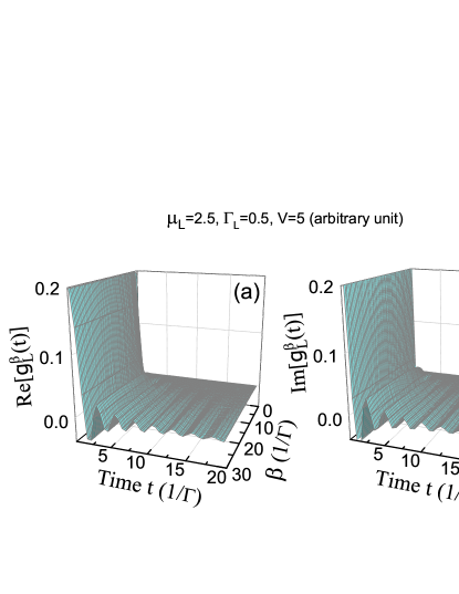
Figure 1: (Color online) 3D plot of temperature-dependent non-local time correlation function $g^{\beta}_{L}(t-\tau)$ (in unit: $\Gamma^{2}$) as a function of temperature for $\mu_{L}=2.5\Gamma$ and $\Gamma_{L}=0.5\Gamma$.

Figure 2: The temperature-dependent non-local time correlation function $g^{\beta}_{L}(t-\tau)$ with different bias voltages at a fixed temperature $\beta^{-1}=k_{\rm B}T=0.1\Gamma$ and $\Gamma_{L}=0.5\Gamma$. The plots of (a) and (b) for $\mu_{L}=0.5\Gamma$, (c) and (d) for $\mu_{L}=30\Gamma$ (the large bias limit).

To examine if some non-Markovian effect can still survive in the WBL, we numerically calculate the transient current passing through the single level resonant tunneling nanostructure considered in the last subsection. In the sequential tunneling regime $\mu_{L}>\epsilon>\mu_{R}$, the exact solutions to the occupation and the transient current are close to the Markov limit (differing by a few present except for a very short time scale from the beginning), as shown in Fig. 3(a)-(d). While, in the co-tunneling regime with $\mu_{\alpha}\gg\epsilon$, the exact solution of the occupation and the current are still almost the same as their Markov solution except for the very short time scale from the beginning, see Fig. 3(e)-(f). These results indicate that the WBL (an extremely short character time of the reservoirs) will dominatively suppress the thermal timescales. In other words, when the line width $W\rightarrow\infty$, not only for the high temperature and large bias limit, but even for a finite temperature and a finite bias voltage, the non-Markovian effects becomes quite weak that are most likely negligible in experiments. Thus the WBL mainly takes into account the Markov dynamics. The manifestation of the non-Markovian memory structure then should go beyond the WBL.Tu08235311 In Fig. 4, we calculate the transient current with different line widths to demonstrate the non-Markovian effect in transport phenomena. As we can see, the transport dynamics is significantly different from the Markov limit for a small $W$. Increasing the value of $W$ will decrease the memory effect accordingly. When the line width $W\geq 50\Gamma$, the exact solution of the transient current closely approaches to the Markov result that is consistent with the WBL. A analysis of the non-Markovian dynamics in this simple resonant tunneling system has also recently been studied using Heisenberg equations of motion.Sch09032110

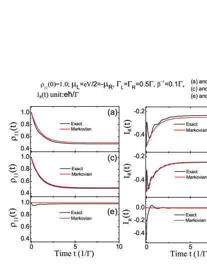
Figure 3: (Color online) Comparison of the non-Markovian dynamics with Markov limit in the WBL for the electron occupation (left row) and the transient current (right row). Here we take the parameters $\Gamma_{L}=\Gamma_{R}=0.5\Gamma$, $\beta^{-1}=k_{\rm B}T=0.1\Gamma$, $\mu_{L,R}=\pm eV/2=\pm 5\Gamma$, and (a)-(b): $eV=10\Gamma$, $\epsilon=2\Gamma$; (c)-(d): $eV=20\Gamma$, $\epsilon=2\Gamma$; (e)-(f): $eV=10\Gamma$, $\epsilon=-10\Gamma$.

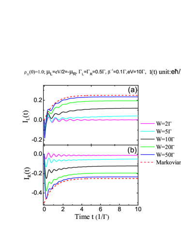
Figure 4: (Color online) The transient current $J_{L,R}(t)$ through the left and right leads with a Lorentzian-type spectral density for different bandwidths: dashed line, the WBL ($W=\infty$), other lines, from the top to bottom for (a) and from the bottom to top for (b), correspond to $W=50\Gamma,20\Gamma,10\Gamma,5\Gamma,2\Gamma$, respectively. Other parameters we used are $\Gamma_{L}=\Gamma_{R}=0.5\Gamma$, $\beta^{-1}=k_{\rm B}T=0.1\Gamma$, $\mu_{L,R}=\pm eV/2=\pm 5\Gamma$, and $\epsilon=2\Gamma$.

IV.3 Transient transport dynamics with time-dependent bias voltage

We are now in the position to study the transient transport phenomena in response to time-dependent bias voltages. The calculation of the time-dependent electron current in response to time-dependent bias voltages has received a great attention recently, through various different theoretical approaches.Jau945528 ; Bru941076 ; Kon9616820 ; Sun004754 ; Zhu03224413 ; And05196801 ; Mac06085324 ; Wei08195316 ; Sch08235110 ; Zhe09164708 ; Hau98 Transient transport dynamics is also a central ingredient in many different experiments, such as single-electron pumps and turnstiles with time-modified gate signals moving electrons one by one through quantum dots,Kir92 ; Swi991905 ; Blu07343 ; Fuj041323 ; Fuj08042102 and the study of the quantum capacitance and inductances with ac voltage response.Nig06206804 ; Wan07155336 ; Zhe07195127 ; Zhe08184112 ; Mo09355301 All these problems can be studied explicitly in the present theory now. The corresponding nanoscale devices can be modelled as a resonant tunneling nanostructure considered in this section. The applying time-dependent voltages are taken to be the most commonly interesting ones. For time-dependent voltages, as we mentioned in Sec. II the single particle energy levels of the leads are changed to $\epsilon_{\alpha k}(t)=\epsilon_{\alpha k}+eV_{\alpha}(t)$. The non-local time correlation functions of the leads can be expressed as

$$g_{\alpha}(\tau,\tau^{\prime}) =\exp\left\{-ie\int^{\tau}_{\tau^{\prime}}d\tau_{1}V_{\alpha}(\tau_{1})\right\}g_{\alpha}(\tau-\tau^{\prime}),$$ (52a)

$$g^{\beta}_{\alpha}(\tau,\tau^{\prime}) =\exp\left\{-ie\int^{\tau}_{\tau^{\prime}}d\tau_{1}V_{\alpha}(\tau_{1})\right\}g^{\beta}_{\alpha}(\tau-\tau^{\prime}).$$ (52b)

With the parametrization of Eq. (48), it is not difficult to numerically calculate the transient electron dynamics for arbitrary line width $W_{\alpha}$. In the following calculation, we set the symmetric ac voltages, i.e., $\mu_{L}(t)=eV(t)/2$ and $\mu_{R}(t)=-eV(t)/2$. For the quantum dot with a single level, the reduced density matrix can be fully characterized by the electron occupation in the dot. The exact numerical results for the transient current and occupation due to different types of applied ac voltages are presented as follows.

Exponentially time-dependent bias voltage

We shall first study the transient transport dynamics in response to an exponentially time-dependent bias voltage $V(t)=V(1-e^{-t/\tau})$, where $\tau>0$ is a time dominating switch-on rate of the voltage. The asymptotic limit $\tau\rightarrow 0^{+}$ corresponds to a step function. The numerical results are plotted in Fig. 5.

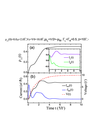
Figure 5: (Color online) The occupation and transient current response to exponential time-dependent voltage with $\tau=1.5/\Gamma$. The other parameters are $eV=10\Gamma$, $\Gamma_{L}=\Gamma_{R}=1.5\Gamma$, $\beta^{-1}=k_{\rm B}T=0.1\Gamma$, $W_{L}=W_{R}=W=20\Gamma$ and $\epsilon=2\Gamma$.

The first peak shown in the displacement current arises from the cotunneling process during the initially short time scale. At beginning, the Fermi surface of the both leads are nearly equivalent to zero and the dot energy level is higher than the Fermi surface. The initial currents through both leads are equal to each other due to the totally symmetric structure. This leads to a zero initial net current. This feature is common for other type of ac bias voltages discussing later. In general, the emergence of the peaks in the current corresponds to a steep transient behavior of the electron states (i.e. the occupation for the single-level dot) occurs inside the dot. The non-linear response to the time-dependent bias is clearly manifested in the change of both the electron state in the dot and the transient current through the leads (including the individual current through each lead and the displacement and net currents), as we plotted in the Fig. 5. In particular, the net current changes in time that closely follows the change of electron occupation in the dot, while the displacement current depicts the steep change rate of the occupation, as we expected from Eq. (28).

Oscillating bias voltage

Now let us move to the transient dynamics driven by an oscillating voltage:Hau98 $V(t)=V_{0}-V_{c}\cos(\omega_{c}t)$, where $V_{0}$ is a dc component, and $V_{c}$ and $\omega_{c}$ are the oscillation amplitude and frequency of the ac component. The corresponding exact numerical solution is shown in Fig. 6.

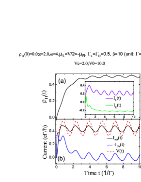
Figure 6: (Color online) The occupation and transient current response to oscillating voltage with the dc component $eV_{0}=10\Gamma$, the ac component $eV_{c}=2\Gamma$ and the oscillating frequency $\omega_{c}=4\Gamma$. The other parameters are the same as in Fig. 5.

As one can see all the quantities, the electron state in the dot and the transient currents, have the similar oscillation behavior as the ac voltage oscillation, where the steady-state values and the oscillation around the steady-state values are determined by the dc voltage $V_{0}$. The oscillation amplitude around the steady-state is proportional to the ac voltage amplitude $V_{c}$ and the oscillation periodic is mainly given by $T=2\pi/\omega_{c}$. However, the transient dynamics of the occupation and current does not always strictly follow the ac voltage oscillation. The current oscillation is a little slantwise compared to the ac voltage oscillation. With increasing the amplitude of the ac voltage $V_{c}$ and decreasing the oscillation frequency $\omega_{c}$, a sideband oscillation occurs in the electron occupation as well as in the transient currents as shown in Fig. 7.

Figure 7: (Color online) The transient current (black line) response to the oscillating voltage (the dashed red line) with $eV_{0}=eV_{c}=10\Gamma$ and the oscillating frequency $\omega_{c}=1\Gamma$ for (a) and $\omega_{c}=0.5\Gamma$ for (b). The other parameters are the same as in Fig. 6.

Physically this sideband oscillation is induced by the sinusoidal behavior of the ac voltage. It can be understood analytically under the WBL:Hau98

$$g^{\beta}_{\alpha}(\tau,\tau^{\prime})=\sum_{n_{1},n_{2}}J_{n_{1}}\left({\Delta_{\alpha}\over\omega_{c}}\right)J_{n_{2}}\left({\Delta_{\alpha}\over\omega_{c}}\right)\int\frac{d\omega}{2\pi}\,\Gamma_{\alpha}f_{\alpha}(\omega)e^{-i(\omega+n_{1}\omega_{c})\tau}e^{i(\omega+n_{2}\omega_{c})\tau^{\prime}},$$ (53a)

$$v^{\beta}(t)=\sum_{\alpha,n_{1},n_{2}}J_{n_{1}}\left({\Delta_{\alpha}\over\omega_{c}}\right)J_{n_{2}}\left({\Delta_{\alpha}\over\omega_{c}}\right)\int\frac{d\omega}{2\pi}\,\Gamma_{\alpha}f_{\alpha}(\omega)\frac{e^{-\Gamma t}+e^{-i(n_{1}-n_{2})\omega_{c}t}-e^{-{\Gamma\over 2}t}\left[e^{-i(\epsilon-\omega-n_{2}\omega_{c})t}+e^{i(\epsilon-\omega-n_{1}\omega_{c})t}\right]}{(\epsilon-\omega-n_{1}\omega_{c})(\epsilon-\omega-n_{2}\omega_{c})+({\Gamma\over 2})^{2}-i{\Gamma\over 2}(n_{1}-n_{2})\omega_{c}},$$ (53b)

$$I_{\alpha}(t)=-\Gamma_{\alpha}\left\{(e^{-\Gamma t}N(t_{0})+{\rm Re}[v^{\beta}(t)]\right\}+\sum_{n_{1},n_{2}}J_{n_{1}}\left({\Delta_{\alpha}\over\omega_{c}}\right)J_{n_{2}}\left({\Delta_{\alpha}\over\omega_{c}}\right)\int\frac{d\omega}{2\pi}\,\Gamma_{\alpha}f_{\alpha}(\omega)2{\rm Im}\frac{e^{-i(\epsilon-\omega-n_{2}\omega_{c})t}-e^{-i(n_{1}-n_{2})\omega_{c}t}}{\epsilon-\omega-n_{2}\omega_{c}+i{\Gamma\over 2}}.$$ (53c)

where the Bessel function satisfies $J_{-n}(z)=(-1)^{n}J_{n}(z)$ and $\Delta_{L,R}=\mp\frac{eV_{c}}{2}$.

Gaussian pulse

The last example we shall study is the transient dynamics droven by a Gaussian pulse $V(t)=V\exp\{-\frac{(t-\tau_{1})^{2}}{\tau^{2}_{2}}\}$. The width and the center of the pulse are determined by $\tau_{2}$ and $\tau_{1}$, respectively. The exact numerical result plotted in Fig. 8 shows that the net current peak emerges (a slightly delay) just after the voltage pulse while the corresponding response of the electron occupation delays significantly. This behavior is easy to be understood that the external voltage pulse leads to a sharp change of the electron occupation due to the delay response. The shape change of the transient current comes from the largest change rate of the electron occupation in the dot. The delay response effect is determined by the tunneling rate $\Gamma$. Outside the voltage pulse, the tunneling current comes completely from the cotunneling effect and the occupation in the dot decays to a stationary value.

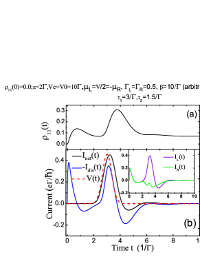
Figure 8: (Color online) The occupation and transient current responses to Gaussian voltage pulse with $\tau_{1}=3/\Gamma$ and $\tau_{2}=0.5/\Gamma$. The other parameters are the same as in Fig. 5.

It is interesting to note that the response of the occupation and the currents to the cotunneling process is different before and after the voltage pulse. Before the voltage pulse, the system is dominated by the cotunneling process because the Fermi surface of the both leads are nearly equivalent but is lower than the dot energy level ($\mu_{L}\simeq\mu_{R}\simeq 0<\epsilon=2\Gamma$). The aligned fermi surfaces double the peak amplitude of the displacement current which also gives the zero net current, while the occupation has a corresponding change regarding the change of the displacement current. With the voltage increasing, the Fermi surface of the left lead moves up over the dot energy level while that of the right lead moves down below the dot energy level such that the system gradually approaches the sequential tunneling regime. This drives the electron flowing from the left lead to the dot and then to the right lead. Such a process results in a sensitive response of all physical quantities, the electron occupation in the dot, the displacement and the net currents. Then with the voltage decaying to zero, the electron residing in the dot is favorable to cotunnel to the left lead which gives a negative current and finally reaches the steady-state. The transient electron dynamics with the non-linear response to this Gaussian pulse is in particular useful for quantum feedback control to the electron states in the dot through the transient current that we will study in the future. It is also favorable to study the quantum capacitance and inductances.Zhe08184112 ; Mo09355301

Note that the above transient dynamics starts with a zero initial occupation, i.e., $\rho_{00}(t_{0})=1$ and $\rho_{11}(t_{0})=1-\rho_{00}(t_{0})=0$ [$N(t_{0})=0$]. This implies that the last term of Eq. (30) which is often ignored in the nonequilibrium Green function techniqueJau945528 ; Mac06085324 has no contribution to the transient current in the above numerical calculations. If the dot is initially occupied, the transient current will be quite different although the steady-state limit is the same because the initial electron distribution vanishes in the steady-state limit. In Fig. 9, we show the exact numerical result with such a situation where we take the simple step-pulse voltage as an example. It shows that the initial occupation in the central region has measurable contributions in studying the transient dynamics, especially for the ultrafast (extremely short time) operations in a quantum device.

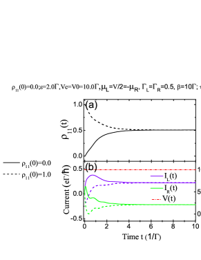
Figure 9: (Color online) The occupation and transient current response to step pulse voltage (i.e. a constant bias after $t=0$, the dot-dashed line) for the initial condition of $\rho_{11}(t_{0})=0$ (solid lines) and $\rho_{11}(t_{0})=1.0$ (dashed lines), respectively. The other parameters are the same as in Fig. 5.

Combining all these analysis together, as one can see the exact numerical solutions presented here have demonstrated that both the electron states in the dot and the transient currents past through it have a clear non-linear response to the external bias voltage pulses, in particular within a short time scale after the pulse is turned on. These ultrafast non-linear response properties will provide very useful information for the manipulation of the device states as well as the quantum feedback controls for practical applications. However, since we only consider here a very simple device with a single-level dot, the quantum coherence and decoherence dynamics to the transient current do not be manifested in these numerical solutions. To demonstrate the quantum coherence properties in the transient transport dynamics, it is necessary to have the device containing at least two levels (or a single level with electron spin degrees of freedom) in the central region. Also, in the above numerical calculations, we take a rather large finite line width, $W_{\alpha}=20\Gamma$. The non-Markovian memory structure will become more significant when the line width becomes narrower.Mac06085324 ; Tu08235311 We will examine in detail these features within the present theory in our future work.

V Summary and prospective

In summary, we have established a nonequilibrium theory for the transient quantum transport dynamics via the Feynman-Vernon influence functional approach. We obtain an analytical relation between the master equation, Eq. (8), and the transient current, Eq. (19), determined by the same time-dependent (non-Markovian) coefficients. In particular, the master equation and the transient current are explicitly related to each other in terms of the superoperators acting on the reduced density matrix of the central system, see Eq. (23). The back-reaction effect of the gating electrodes to the central system is fully taken into account by the time-dependent coefficients in the master equation (8) through the dissipation-fluctuation integrodifferential equation (7). The non-Markovian memory structure is non-perturbatively built into the integral kernels in these equations of motion. The resulting transient current, Eq. (19) or (30), is rather simple and it recovers the steady-state current in the nonequilibirum Green function technique and the Landauer-Büttiker formula at the long time limit. This exact nonequilibrium formalism should provide a very intuitive picture of how the change of the electron quantum coherence in the central system is intimately related with the electron tunneling processes through the leads, and therefore non-linearly responses to the corresponding external bias controls. This theory is applicable to study a variety of quantum transport phenomena involving explicitly non-Markovian quantum decoherence behaviors, in both stationary and transient scenarios, at arbitrary temperatures of the different contacts in the weak Coulomb interaction regime.

As a simple illustration, we apply the theory to a simple model of electron tunneling though a single level quantum dot. We obtain all analytical solutions in the wide band limit (WBL) where the dependence of the initial electron occupation in the dot is explicitly manifested. Taking a more realistic spectral density with Lorentzian shape, we show that the Markov limit is a good approximation in the WBL. The non-Markovian memory effect is dominated by a finite line width of the spectral density. Under the ac bias voltage pulses (including the step pulse, the Gaussian pulse and the oscillation pulse), we have demonstrated the ultrafast non-linear response of the electron occupation and currents to the ac bias. We find that the current evolutions are more sensitive to the energetic configuration of the dot than the occupation evolution. This feature is very useful for quantum feedback controls in quantum information processing. More applications will be presented in the future works. These include the decoherence transport dynamics in quantum dot devices such as quantum dot Aharonov-Bohm inteferometers; the nonequilibrium dynamics and the real time monitoring of spin polarization processes in nanostrucutres; also the transient transport dynamics in molecular electronics, as well as the application to bio-electronics such as DNA junctions, etc.

In the end, we should also point out that the present theory is developed without considering the electron-electron interaction in the central region and therefore it is mainly valid in the weak Coulomb interaction regime. It is not difficult to extend the present theory to the strong Coulomb Blockage regime by properly excluding the doubly occupied states in the central region of the nanostructure, as we have shown explicitly in [Tu08235311, ]. Although studying the above two extreme limits, the extremely weak and the extremely strong Coulomb interaction regimes together, could reveal a significant understanding to various quantum transport phenomena, there is increasing discussion for the intermediate Coulomb interaction regime Cha08245412 ; Sch09033302 where the analysis of transport dynamics should become much more complicated. In this situation, the path integrals of Eqs. (3) and (14) may not be carries out exactly, and therefore it is not easy to find an exact master equation and an exact expression of the transient current. But the master equation, Eq. (8), and the transient current, Eq. (19), can still serve as a good approximation with respect to the saddle point approximation or loop expansion,zhang921900 where the Coulomb interaction must be included self-consistently in the dissipation-fluctuation integrodifferential equation (7). This approximate treatment could provide a basic understanding to the quantum transport phenomena in the intermediate Coulomb interaction regime. The detailed extension of the present theory to the interacting electron systems is in progress now. Nevertheless, the analytical nonequilibrium theory we presented in this paper has the advantage of combining the decoherence dynamics with transient transport dynamics together to explore time-dependent physical phenomena and may also provide a basic theory for quantum feedback controls in various nanoelectronics devices.

Appendix A The relations between $\bm{u}(t),\bar{\bm{u}}(\tau)$, $\bm{v}^{\beta}(t)$ and the nonequilibrium Green functions

As we see both the master equation (8) and the transient current (30) are completely determined by the propagating matrices of the stationary paths: $\bm{u}(\tau),\bar{\bm{u}}(\tau)$ and $\bm{v}^{\beta}(\tau)$. Here we shall show that these propagating matrices are directly related to the retarded, advanced and lesser Green functions in the nonequilibrium Green function technique. In our previous work,Tu08235311 the propagating matrices $\bm{u}(\tau),\bar{\bm{u}}(\tau)$ and $\bm{v}^{\beta}(\tau)$ were introduced to simplify the stationary path equations of motion (with the convention $\bm{x}=\bm{y}\bm{z}$ for $x_{i}=\sum_{j}y_{ij}z_{j}$) as follows:

$$\bm{\xi}(\tau)={\bm{u}}(\tau)\bm{\xi}(t_{0})+{\bm{v}}^{\beta}(\tau)[\bm{\xi}(t)+\bm{\xi}^{\prime}(t)],$$ (54a)

$$\bm{\xi}(\tau)+\bm{\xi}^{\prime}(\tau)=\bar{\bm{u}}(\tau)[\bm{\xi}(t)+\bm{\xi}^{\prime}(t)].$$ (54b)

In fact, Eq. (54) shows that $\bm{u}(\tau)$ is a propagating matrix of the forward stationary paths $\bm{\xi}(\tau)$ starting at $t_{0}$, while $\bm{v}^{\beta}(\tau)$ mixes the forward path $\bm{\xi}(\tau)$ and the backward path $\bm{\xi}^{\prime}(\tau)$ started backwardly from $t$, and $\bar{\bm{u}}(\tau)$ is a backward propagating matrix of the stationary paths. In fact, Eq. (54) shows that the transformation matrices $\bm{u}(\tau),\bar{\bm{u}}(\tau)$ and $\bm{v}^{\beta}(\tau)$ should be defined more precisely as $\bm{u}(\tau)\equiv{\sf u}(\tau,t_{0})$, $\bar{\bm{u}}(\tau)\equiv{\sf u}^{\dagger}(t,\tau)$ and $\bm{v}^{\beta}(\tau)\equiv{\sf v}^{\beta}(\tau,t)$:

$$\bm{\xi}(\tau)={\sf u}(\tau,t_{0})\bm{\xi}(t_{0})+{\sf v}^{\beta}(\tau,t)[\bm{\xi}(t)+\bm{\xi}^{\prime}(t)],$$ (55a)

$$\bm{\xi}(\tau)+\bm{\xi}^{\prime}(\tau)={\sf u}^{\dagger}(t,\tau)[\bm{\xi}(t)+\bm{\xi}^{\prime}(t)],$$ (55b)

where the Grassmannian variables $\bm{\xi}(\tau)$ and $\bm{\xi}^{\prime}(\tau)$ represent the forward and backward electron paths in the functional path integrals. Then Eq. (54) directly tells that ${\sf u}(\tau,t_{0})$ describes the electron propagation (represented by $\bm{\xi}(\tau)$ in the Grassmannian space) from the initial time $t_{0}$ to the time $\tau$ so that it is just the retarded Green function, namely,

$$\bm{u}(\tau) ={\sf u}(\tau,t_{0})=i\bm{G}^{r}(\tau,t_{0})$$

$$=\theta(\tau-t_{0})\langle\{a_{i}(\tau),a^{\dagger}_{j}(t_{0})\}\rangle.$$ (56)

Eq. (33) is a justification for this relation. While, ${\sf u}^{\dagger}(t,\tau)$ describes the inverse propagation of the electron [or the backward propagation represented by $\bm{\xi}^{\prime}(\tau)$] from the time $t$ to the time $\tau$ such that it is indeed the advanced Green function:

$$\bar{\bm{u}}(\tau)={\sf u}^{\dagger}(t,\tau)=-i\bm{G}^{a}(\tau,t).$$ (57)

Meantime, Eq. (7a) indicates that the time correlation function of the $\alpha$-reservoir:

$$\bm{g}_{\alpha ij} (\tau_{1},\tau_{2})=i\bm{\Sigma}_{\alpha ij}^{r}(\tau_{1},\tau_{2})$$

$$=\theta(\tau_{1}-\tau_{2})\sum_{k}V_{\alpha ki}V^{\ast}_{\alpha kj}\langle\{c_{\alpha k}(\tau_{1}),c^{\dagger}_{\alpha k}(\tau_{2})\}\rangle_{\mbox{\tiny B}},$$ (58)

as a back-reaction effect of the $\alpha$-lead to the central system, is the retarded self-energy. These relations are also justified by Eqs. (7a-7b).

The function ${\sf v}^{\beta}(\tau,t)$ describes the electron propagation mixing the forward and backward paths so that it is related to the lesser Green function defined by $\bm{G}^{<}_{ij}(\tau,t)\equiv i\langle a^{\dagger}_{j}(t)a_{i}(\tau)\rangle$ in the nonequilibrium Green function formalism. In fact, it is not difficult to find the explicit solution of Eq. (7c):

$$\bm{v}^{\beta}(\tau)={\sf v}^{\beta}(\tau,t)= \int^{\tau}_{t_{0}}d\tau_{1}\int_{t_{0}}^{t}d\tau_{2}~{}{\sf u}(\tau,\tau_{1})\bm{g}^{\beta}(\tau_{1},\tau_{2}){\sf u}^{\dagger}(t,\tau_{2})$$ (59)

which in terms of Green functions becomes

$${\sf v}^{\beta}(\tau,t)= -i\int^{\tau}_{t_{0}}d\tau_{1}\int_{t_{0}}^{t}d\tau_{2}~{}\bm{G}^{r}(\tau,\tau_{1})\bm{\Sigma}^{<}(\tau_{1},\tau_{2})\bm{G}^{a}(\tau_{2},t),$$ (60)

where

$$\bm{\Sigma}^{<}(\tau_{1},\tau_{2})=i\bm{g}^{\beta}(\tau_{1},\tau_{2}),$$ (61)

is the lesser component of the self-energy. On the other hand, the single-particle reduced density matrix is related to the lesser Green function by $\bm{\rho}^{(1)}(t)=-i\bm{G}^{<}(\tau,t)|_{\tau=t}$. From the relation of Eq. (29), we find that $\bm{v}^{\beta}(\tau)$ can be expressed in terms of the lesser Green function as follows:

$$\bm{G}^{<}(\tau,t)= i[\bm{u}(\tau)\bm{\rho}^{(1)}(t_{0})\bm{u}^{\dagger}(t)+{\bm{v}}^{\beta}(\tau)]$$

$$= \bm{G}^{r}(\tau,t_{0})\bm{G}^{<}(t_{0},t_{0})\bm{G}^{a}(t_{0},t)$$

$$+\int^{\tau}_{t_{0}}d\tau_{1}\int_{t_{0}}^{t}d\tau_{2}~{}\bm{G}^{r}(\tau,\tau_{1})\bm{\Sigma}^{<}(\tau_{1},\tau_{2})\bm{G}^{a}(\tau_{2},t).$$ (62)

This provides indeed a general solution of the lesser Green function in the nonequilibrium Green function technique. In the previous investigation of transient dynamics, the first term in Eq. (62) that sensitively depends on the initial electron distribution in the central regions are often ignored.Jau945528 ; Hau98 ; Mac06085324 In fact, the second term in Eq. (62) can only be identified as the lesser Green function $\bm{G}^{<}(\tau,t)$ in the steady-state limit.

Using the above explicit relations between $\bm{u}(t),\bar{\bm{u}}(\tau)$, $\bm{v}^{\beta}(t)$ and the nonequilibrium retarded, advanced and lesser Green functions, we immediately obtain the transient current of Eq. (30) in terms of the nonequilibrium Green functions:

$$I_{\alpha}(t)=-\frac{2e}{\hbar}{\rm Re}\int_{t_{0}}^{t}\!d\tau\,{\rm Tr}\Big{\{} \bm{\Sigma}^{r}_{\alpha}(t,\tau)\bm{G}^{<}(\tau,t)$$

$$+\bm{\Sigma}^{<}_{\alpha}(t,\tau)\bm{G}^{a}(\tau,t)\Big{\}}.$$ (63)

This current has exactly the same form obtained form the nonequilibrium Green function technique.Jau945528 ; Hau98 However, as we have pointed out in the practical applications, one usually uses the steady-state lesser Green function, namely ignoring the first term in Eq. (62). This term vanishes in the steady-state limit so that it will not affect the steady-state current. It can also be dropped if one takes the initial time $t_{0}\rightarrow-\infty$ so that the central region is assumed to be in an empty state initially. However, this term which explicitly depends on the initial single particle reduced density matrix (including the initial electron occupation in each level and the electron quantum coherence between different levels in the central region) is crucial for practical manipulation of a real quantum device. Only in the wide band limit (WBL) where the non-local time correlation function

$$\bm{g}_{\alpha}(t,\tau)=i\bm{\Sigma}^{r}_{\alpha}(t,\tau)=\bm{\Gamma}_{\alpha}\delta(t-\tau),$$ (64)

the integral of the first term in Eq. (63) is reduced to the single particle reduced density matrix: $\bm{G}^{<}(t,t)=i\bm{\rho}^{(1)}(t)$), which results in

$$I_{\alpha}(t)= -\frac{e}{\hbar}{\rm Tr}\Big{[}\bm{\Gamma}_{\alpha}\bm{\rho}^{(1)}(t)-\bm{\Gamma}_{\alpha}\int\frac{d\omega}{\pi}f_{\alpha}(\omega)$$

$$\times\int^{t}_{t_{0}}d\tau{\rm Im}\big{\{}e^{-i[\omega(t-\tau)+e\int_{\tau}^{t}d\tau^{\prime}V_{\alpha}(\tau^{\prime})]}\bm{G}^{a}(\tau,t)\big{\}}\Big{]}.$$ (65)

Thus, the ignored initial occupation dependence is recovered in the WBL.

References

- (1) D. Goldhaber-Gordon, H. Shtrikman, D. Mahalu, D. Abusch- Magder, U. Meirav, and M. A. Kastner, Nature (London) 391, 156 (1998).
- (2) S. M. Cronenwett, T. H. Oosterkamp, and L. P. Kouwenhoven, Science 281, 540 (1998).
- (3) W. Lu, Z. Ji, L. Pfeiffer, K. W. West, and A. J. Rimberg, Nature (London) 423, 422 (2003).
- (4) T. Hayashi, T. Fujisawa, H. D. Cheong, Y. H. Jeong and Y. Hirayama, Phys. Rev. Lett. 91, 226084 (2003).
- (5) J. R. Petta, A. C. Johnson, J. M. Taylor, E. A. Laird, A. Yacoby, M. D. Lukin, C. M. Marcus, M. P. Hanson, A. C. Gossard. Science 309, 1280 (2005).
- (6) T. Fujisawa, T. Hayashi, and S. Sasaki, Rep. Prog. Phys. 69, 759 (2006).
- (7) R. Hanson, L. P. Kouwenhoven, J. R. Petta, S. Tarucha, and L. M. K. Vandersypen, Rev. Mod. Phys. 79, 1217 (2007).
- (8) C. Bruder, and H. Schoeller, Phys. Rev. Lett. 72, 1076 (1994).
- (9) J. König, J. Schmid, H. Schoeller, and G. Schön, Phys. Rev. B 54, 16820 (1996).
- (10) N. S. Wingreen, A.-P. Jauho, and Y. Meir, Phys. Rev. B 48, 8487 (1993).
- (11) A.-P. Jauho, N. S. Wingreen, and Y. Meir, Phys. Rev. B 50, 5528 (1994).
- (12) Q.-F. Sun, B.-G. Wang, J. Wang, and T.-H. Lin, Phys. Rev. B 61, 4754 (2000).
- (13) Z.-G. Zhu, G. Su, Q.-R. Zheng, and B. Jin, Phys. Rev. B 68,224413 (2003).
- (14) F. B. Anders and A. Schiller, Phys. Rev. Lett. 95, 196801 (2005).
- (15) X. Q. Li, J. Y. Luo, Y. G. Yang, P. Cui, and Y. J. Yan, Phys. Rev. B 71, 205304 (2005).
- (16) M. T. Lee and M. W. Zhang, Phys. Rev. B 74, 085325 (2006)
- (17) J. Maciejko, J. Wang, and H. Guo, Phys. Rev. B 74, 085324 (2006).
- (18) J. S. Jin, X. Zheng, and Y. J. Yan, J. Chem. Phys. 128, 234703 (2008).
- (19) S. Weiss, J. Eckel, M. Thorwart, and R. Egger, Phys. Rev. B 77, 195316 (2008).
- (20) T. L. Schmidt, P. Werner, L. Muhlbacher, and A. Komnik, Phys. Rev. B 78, 235110 (2008).
- (21) M. W. Y. Tu and W. M. Zhang, Phys. Rev. B 78, 235311 (2008).
- (22) P. Zedler, G. Schaller, G. Kiesslich, C. Emary, and T. Brandes, Phys. Rev. B 80, 045309 (2009).
- (23) X. Zheng, J. S. Jin, S. Welack, M. Luo and Y. J. Yan, J. Chem. Phys. 130, 164708 (2009).
- (24) H. Haug and A. P. Jauho, Quantum Kinetics in Transport and Optics of Semiconductors, (Springer-Verlag, Berlin, 1998), springer Series in Solid-State Sciences 123.
- (25) K. Huang, Statistical Mechanics, (2Ed, John Wiley & Sons, 1987).
- (26) C. Cercignani, Theory and Application of the Boltzmann Equation, (Scottish Academic Press, Edinburgh, 1975).
- (27) H. Smith, H. H. Jensen, Transport Phenomena, (Clarendon, Oxford, 1989).
- (28) H. J. Carmichael , An Open Systems Approach to Quantum Optics, Lecture Notes in Physics, Vol. m18, (Springer-Verlag, Berlin, 1993).
- (29) H.-P. Breuer and F. Petruccione, The Theory of Open Quantum Systems, (Oxford University Press, Oxford, 2002).
- (30) J. Schwinger, J. Math. Phys. 2, 407 (1961).
- (31) L. P. Kadanoff, G. Baym, Quantum Statistical Mechanics, (Benjamin, New York, 1962)
- (32) L. V. Keldysh, Sov. Phys. JETP, 20, 1018 (1965).
- (33) R. P. Feynman and F. L. Vernon, Ann. Phys. 24, 118 (1963).
- (34) K. C. Chou, Z. B. Su, B. L. Hao, and L. Yu, Phys. Rep. 118, 1 (1985).
- (35) J. Rammer and H. Smith, Rev. Mod. Phys. 58, 323 (1986).
- (36) Y. Meir, N. S. Wingreen, and P. A. Lee, Phys. Rev. Lett. 66, 3048 (1991).
- (37) Y. Meir and N. S. Wingreen, Phys. Rev. Lett. 68, 2512 (1992).
- (38) S. Datta, Electronic Transport in Mesoscopic Systems, (Cambridge, England, 1995).
- (39) A. J. Legget, S. Chakravarty, A. T. Dorsey, M. P. A. Fisher, A. Garg and W. Zwerger, Rev. Mod. Phys. 59, 1 (1987).
- (40) W. H. Zurek, Phys. Today 44 (10), 36 (1991); Rev. Mod. Phys. 75, 715 (2003).
- (41) A. O. Caldeira and A. J. Leggett, Physica A 121, 587 (1983).
- (42) F. Haake, and R. Reibold, Phys. Rev. A 32, 2462 (1985).
- (43) B. L. Hu, J. P. Paz, and Y. H. Zhang, Phys. Rev. D 45, 2843 (1992).
- (44) U. Weiss, Quantum Dissipative Systems, (3rd Ed. World Scientific, Singapore, 2008).
- (45) E. Calzetta and B. L. Hu, Nonequilibrium Quantum Field Theory, (Cambridge University Press, New York, 2008).
- (46) J. H. An and W. M. Zhang, Phys. Rev. A 76, 042127 (2007).
- (47) C. H. Chou, T. Yu, and B. L. Hu, Phys. Rev. E 77, 011112 (2008).
- (48) J. H. An, M. Feng and W. M. Zhang, Quantum Infom. Comput. 9, 0317 (2009).
- (49) T. Yu and J. H. Eberly, Phys. Rev. Lett., 93, 140404 (2004).
- (50) H. Schoeller and G. Schön, Phys. Rev. B 50, 18436 (1994).
- (51) J. König, H. Schoeller, and G. Schön, Phys. Rev. Lett. 76, 1715 (1996).
- (52) M. T. Lee and W. M. Zhang, J. Chem. Phys. 129, 224106 (2008).
- (53) J. Lehmann, S. Kohler, P. Hänggi, and A. Nitzan, Phys. Rev. Lett. 88, 228305 (2002).
- (54) J. N. Pedersen and A. Wacker, Phys. Rev. B 72, 195330 (2005).
- (55) P. Cui, X. Q. Li, J. S. Shao, and Y. J. Yan, Phys. Lett. A 357, 449 (2006).
- (56) S. Welack, M. Schreiber, and U. Kleinekath Lofer, J. Chem. Phys. 124, 044712 (2006).
- (57) U. Harbola, M. Esposito, and S. Mukamel, Phys. Rev. B 74, 235309 (2006).
- (58) X. Zheng, J. S. Jin and Y. J. Yan, New J. Phys. 10, 093016 (2008).
- (59) L. D. Faddeev, Gauge Fields (Benjamin/Cummings, 1980)
- (60) W. M. Zhang, D. H. Feng, and R. Gilmore, Rev. Mod. Phys. 62, 867 (1990).
- (61) Usually the stationary path or stationary phase method is an approximation to path integral calculations. When the path integrals can be reduced to Gaussian integrals, the stationary path method will lead to an exact solution. For more detailed discussion, see R. P. Feynman and A. R. Hibbs, Quantum Mechanics and Path Integrals (McGraw-Hill, 1965).
- (62) J. Fransson, O. Eriksson, and I. Sandalov, Phys. Rev. B 66, 195319 (2002).
- (63) S. A. Gurvitz, Phys. Rev. B 56, 15215 (1997); S. A. Gurvitz and Y. S. Prager, Phys. Rev. B 53, 15932 (1996).
- (64) D. Mozyrsky, L. Fedichkin, S. A. Gurvitz, and G. P. Berman, Phys. Rev. B 66, 161313 (2002).
- (65) C. Flindt, T. Novotn y, and A.-P. Jauho, Phys. Rev. B 70, 205334 (2004); T. Novotn y, A. Donarini, C. Flindt, and A.-P. Jauho, Phys. Rev. Lett. 92, 248302 (2004).
- (66) G. Schaller, P. Zedler, and T. Brandes, Phys. Rev. A 79, 032110 (2009).
- (67) A. Fujiwara, N. M. Zimmerman, Y. Ono, and Y. Takahashi, Appl. Phys. Lett. 84, 1323 (2004).
- (68) A. Fujiwara, K. Nishiguchi, and Y. Ono, Appl. Phys. Lett. 92, 042102 (2008).
- (69) W. P. Kirk and M. A. Reed (Eds.), Nanostructures and Mesoscopic Systems (Academic, San Diego, 1992).
- (70) M. Switkes, C. M. Marcus, K. Campman, and A. C. Gossard, Science 283, 1905 (1999).
- (71) M. D. Blumenthal, B. Kaestner, L. Li, S. Giblin, T. J. B. M. Janssen, M. Pepper, D. Anderson, G. Jones, and D. A. Ritchie, Nature. Phys. 3, 343 (2007).
- (72) X. Zheng, J. S. Jin, and Y. J. Yan, J. Chem. Phys. 129, 184112 (2008).
- (73) S. E. Nigg, R. López, and M. Büttiker, Phys. Rev. Lett. 97, 206804 (2006).
- (74) J. Wang, B. Wang, and H. Guo, Phys. Rev. B 75, 155336 (2007).
- (75) X. Zheng, F. Wang, C. Y. Yam, Y. Mo, and G. H. Chen, Phys. Rev. B 75, 195127 (2007).
- (76) Y. Mo, X. Zheng, G. H. Chen and Y. J. Yan, J. Phys.: Condens. Matter 21, 355301 (2009).
- (77) Y. C. Chang and D. M.-T. Kuo, Phys. Rev. B 77, 245412 (2008).
- (78) M. G. Schultz and F. von Oppen, Phys. Rev. B 80, 033302 (2009).
- (79) W. M. Zhang and L. Wilets, Phys. Rev. C 45, 1900 (1992).