Geometric Arbitrage Theory and Market Dynamics Reloaded

Abstract

This paper is essentially a new version of [Fa15], where some flaws have been amended. We have embedded the classical theory of stochastic finance into a differential geometric framework called Geometric Arbitrage Theory and show that it is possible to:

• Write arbitrage as curvature of a principal fibre bundle.

• Parameterize arbitrage strategies by its holonomy.

• Give the Fundamental Theorem of Asset Pricing a differential homotopic characterization.

• Characterize Geometric Arbitrage Theory by five principles and show they are consistent with the classical theory of stochastic finance.

• Derive for a closed market the equilibrium solution for market portfolio and dynamics in the cases where:

  • Arbitrage is allowed but minimized.

  • Arbitrage is not allowed.

• Prove that the no-free-lunch-with-vanishing-risk condition implies the zero curvature condition. The converse is in general not true and additionally requires the Novikov condition for the instantaneous Sharpe Ratio to be satisfied.

1 Introduction

This paper develops a conceptual structure - called Geometric Arbitrage Theory or GAT - embedding the classical stochastic finance into a stochastic differential geometric framework. The main contribution of this approach consists of modelling markets made of basic financial instruments together with their term structures as principal fibre bundles. Financial features of this market - like no arbitrage and equilibrium - are then characterized in terms of standard differential geometric constructions - like curvature - associated to a natural connection in this fibre bundle or to a stochastic Lagrangian structure that can be associated to it.
Several research areas can benefit from the GAT approach:

• Risk management, with the development of a consistent scenario generators reducing the complexity of the market, while maintaining the fundamental connections between financial instruments and allowing for a reconciliation of econometric forecasting with SDEs techniques. See Smith and Speed ([SmSp98]).

• Pricing, hedging and statistical arbitrage, with the development of generalized Black-Scholes equations accounting for arbitrage and the computation of positive arbitrage strategies in intraday markets. See Farinelli and Vazquez ([FaVa12]) for a practical application leading to an almost one probability growth portfolios with real assets.

Principal fibre bundle theory has been heavily exploited in theoretical physics as the language in which laws of nature can be best formulated by providing an invariant framework to describe physical systems and their dynamics. These ideas can be carried over to mathematical finance and economics. A market is a financial-economic system that can be described by an appropriate principle fibre bundle. A principle like the invariance of market laws under change of numéraire can be seen then as gauge invariance. The fact that gauge theories are the natural language to describe economics was first proposed by Malaney and Weinstein in the context of the economic index problem ([Ma96], [We06]). Ilinski (see [Il00] and [Il01]) and Young ([Yo99]) proposed to view arbitrage as the curvature of a gauge connection, in analogy to some physical theories. Independently, Cliff and Speed ([SmSp98]) further developed Flesaker and Hughston seminal work ([FlHu96]) and utilized techniques from differential geometry (indirectly mentioned by allusive wording) to reduce the complexity of asset models before stochastic modelling. Perhaps due to its borderline nature lying at the intersection between stochastic finance and differential geometry, there was almost no further mathematical research, and the subject, unfairly considered as an exotic topic, remained confined to econophysics, (see [FeJi07], [Mo09] and [DuFiMu00]). We would like to demonstrate that Geometric Arbitrage Theory can be given a rigorous mathematical background and can bring new insights to mathematical finance by looking at the same concepts from a different perspective. That for we will utilize the formal background of stochastic differential geometry as in Schwartz ([Schw80]), Elworthy ([El82]), Eméry ([Em89]), Hackenbroch and Thalmaier ([HaTh94]), Stroock ([St00]) and Hsu ([Hs02]).

This paper is structured as follows. In Section 2, after an introductory review of classical stochastic finance, the primitives of Geometric Arbitrage Theory are explained. Section 3 develops the foundations of GAT, allowing an interpretation of arbitrage as curvature of a principal fibre bundle representing the market and defining the quantity of arbitrage associated to a market or to a self-financing strategy. The no-free-lunch-with-vanishing-risk (or NFLVR for short) condition implies the vanishing of the curvature. The converse is in general not true and additionally requires the instantaneous Sharpe Ratio for the asset value dynamics to satisfy the Novikov condition. The NFLVR condition has the interpretation of a continuity equation satisfied by value density and current of the market, as fluid density and current in the hydrodynamics of an incompressible flow. If all market agents follow the principle of expected utility maximization, then the curvature vanishes and viceversa. Section 4 provides a guiding example for a market whose asset prices are Itô processes. In Section 5 the connections between mathematical finance and differential topology are analyzed. Homotopic equivalent self-financing arbitrage strategies can be parameterized by the Lie algebra of the holonomy group of the principal fibre bundle. The no-free-lunch-with-vanishing-risk condition is seen to be equivalent to the triviality of the holonomy group or to the triviality of the homotopy group. This is a differential-homotopic formulation of the Fundamental Theorem of Asset Pricing. In Section 6 we express the market model in terms of a stochastic Lagrangian system, whose dynamics is given by the stochastic Euler-Lagrange Equations. Symmetries of the Lagrange function can be utilized to derive first integrals of the dynamics by means of the stochastic version of Nöther’s Theorem. Equilibrium and non-equilibrium solutions are explicitly computed. Section 7 concludes.

2 Geometric Arbitrage Theory Fundamentals

2.1 The Classical Market Model

In this subsection we will summarize the classical set up, which will be rephrased in Section 3 in differential geometric terms. We basically follow [HuKe04] and the ultimate reference [DeSc08].

We assume continuous time trading and that the set of trading dates is $[0,+\infty[$. This assumption is general enough to embed the cases of finite and infinite discrete times as well as the one with a finite horizon in continuous time. Note that while it is true that in the real world trading occurs at discrete times only, these are not known a priori and can be virtually any points in the time continuum. This motivates the technical effort of continuous time stochastic finance.

The uncertainty is modelled by a filtered probability space $(\Omega,\mathcal{A},\mathbb{P})$, where $\mathbb{P}$ is the statistical (physical) probability measure, $\mathcal{A}=(\mathcal{A}_{t})_{t\in[0,+\infty[}$ an increasing family of sub-$\sigma$-algebras of $\mathcal{A}_{\infty}$ and $(\Omega,\mathcal{A}_{\infty},\mathbb{P})$ is a probability space. The filtration $\mathcal{A}$ is assumed to satisfy the usual conditions, that is

• right continuity: $\mathcal{A}_{t}=\bigcap_{s>t}\mathcal{A}_{s}$ for all $t\in[0,+\infty[$.

• $\mathcal{A}_{0}$ contains all null sets of $\mathcal{A}_{\infty}$.

The market consists of finitely many assets indexed by $j=1,\dots,N$, whose nominal prices are given by the vector valued semimartingale $S:[0,+\infty[\times\Omega\rightarrow\mathbf{R}^{N}$ denoted by $(S_{t})_{t\in[0,+\infty[}$ adapted to the filtration $\mathcal{A}$. The stochastic process $(S^{j}_{t})_{t\in[0,+\infty[}$ describes the price at time $t$ of the $j$th asset in terms of unit of cash at time $t=0$. More precisely, we assume the existence of a $0$th asset, the cash, a strictly positive semimartingale, which evolves according to $S_{t}^{0}=\exp(\int_{0}^{t}du\,r^{0}_{u})$, where the integrable semimartingale $(r^{0}_{t})_{t\in[0,+\infty[}$ represents the continuous interest rate provided by the cash account: one always knows in advance what the interest rate on the own bank account is, but this can change from time to time. The cash account is therefore considered the locally risk less asset in contrast to the other assets, the risky ones. In the following we will mainly utilize discounted prices, defined as $\hat{S}_{t}^{j}:=S_{t}^{j}/S^{0}_{t}$, representing the asset prices in terms of current unit of cash.

We remark that there is no need to assume that asset prices are positive. But, there must be at least one strictly positive asset, in our case the cash. If we want to renormalize the prices by choosing another asset instead of the cash as reference, i.e. by making it to our numéraire, then this asset must have a strictly positive price process. More precisely, a generic numéraire is an asset, whose nominal price is represented by a strictly positive stochastic process $(B_{t})_{t\in[0,+\infty[}$, and which is a portfolio of the original assets $j=0,1,2,\dots,N$. The discounted prices of the original assets are then represented in terms of the numéraire by the semimartingales $\hat{S}_{t}^{j}:=S_{t}^{j}/B_{t}$.

We assume that there are no transaction costs and that short sales are allowed. Remark that the absence of transaction costs can be a serious limitation for a realistic model. The filtration $\mathcal{A}$ is not necessarily generated by the price process $(S_{t})_{t\in[0,+\infty[}$: other sources of information than prices are allowed. All agents have access to the same information structure, that is to the filtration $\mathcal{A}$.

A strategy is a predictable stochastic process $x:[0,+\infty[\times\Omega\rightarrow\mathbf{R}^{N}$ describing the portfolio holdings. The stochastic process $(x^{j}_{t})_{t\in[0,+\infty[}$ represents the number of pieces of $j$th asset portfolio held by the portfolio as time goes by. Remark that the Itô stochastic integral

$$\int_{0}^{t}x\cdot dS=\int_{0}^{t}x_{u}\cdot dS_{u},$$ (1)

and the Stratonovich’s stochastic integral

$$\int_{0}^{t}x\circ dS:=\int_{0}^{t}x\cdot dS+\frac{1}{2}\int_{0}^{t}d\left<x,S\right>=\int_{0}^{t}x_{u}\cdot dS_{u}+\frac{1}{2}\int_{0}^{t}d\left<x,S\right>_{u}$$ (2)

are well defined for this choice of integrator ($S$) and integrand ($x$), as long as the strategy is admissible. We mean by this that $x$ is a predictable semimartingale for which the Itô integral $\int_{0}^{t}x\cdot dS\geq-v$ is a.s. for some $v>0$ and all $t$. Thereby, the bracket $\left<\cdot,\cdot\right>$ denotes the continuous part of the quadratic covariation of two processes. In a general context strategies do not need to be semimartingales, but if we want the quadratic covariation in (2) and hence Stratonovich’s integral to be well defined, we must require this additional assumption. For details about stochastic integration we refer to Appendix A in [Em89], which summarizes Chapter VII of the authoritative [DeMe80]. The portfolio value is the process $(V_{t})_{t\in[0,+\infty[}$ defined by

$$V_{t}:=V_{t}^{x}:=x_{t}\cdot S_{t}.$$ (3)

An admissible strategy $x$ is said to be self-financing if and only if the portfolio value at time $t$ is given by

$$V_{t}=V_{0}+\int_{0}^{t}x_{u}\cdot dS_{u}.$$ (4)

This means that the portfolio gain is the Itô integral of the strategy with the price process as integrator: the change of portfolio value is purely due to changes of the assets’ values. The self-financing condition can be rewritten in differential form as

$$dV_{t}=x_{t}\cdot dS_{t}.$$ (5)

As pointed out in [BjHu05], if we want to utilize Stratonovich’s integral to rephrase the self-financing condition, while maintaining its economical interpretation (which is necessary for the subsequent constructions of mathematical finance), we write

$$V_{t}=V_{0}+\int_{0}^{t}x_{u}\circ dS_{u}-\frac{1}{2}\int_{0}^{t}d\left<x,S\right>_{u}$$ (6)

or, equivalently

$$dV_{t}=x_{t}\circ dS_{t}-\frac{1}{2}\,d\left<x,S\right>_{t}.$$ (7)

An arbitrage strategy (or arbitrage for short) for the market model is an admissible self-financing strategy $x$, for which one of the following condition holds for some horizon $T>0$:

• $P[V_{0}^{x}<0]=1$ and $P[V_{T}^{x}\geq 0]=1$,

• $P[V_{0}^{x}\leq 0]=1$ and $P[V_{T}^{x}\geq 0]=1$ with $P[V_{T}^{x}>0]>0$.

In Chapter 9 of [DeSc08] the no arbitrage condition is given a topological characterization. In view of the fundamental Theorem of asset pricing, the no-arbitrage condition is substituted by a stronger condition, the so called no-free-lunch-with-vanishing-risk.

Definition 1.

Let $(S_{t})_{t\in[0,+\infty[}$ be a semimartingale and $(x_{t})_{t\in[0,+\infty[}$ and admissible strategy. We denote by $(x\cdot S)_{+\infty}:=\lim_{t\rightarrow+\infty}\int_{0}^{t}x_{u}\cdot dS_{u}$, if such limit exists, and by $K_{0}$ the subset of $L^{0}(\Omega,\mathcal{A}_{\infty},P)$ containing all such $(x\cdot S)_{+\infty}$. Then, we define

• $C_{0}:=K_{0}-L^{0}_{+}(\Omega,\mathcal{A}_{\infty},\mathbb{P})$.

• $C:=C_{0}\cap L^{\infty}_{+}(\Omega,\mathcal{A}_{\infty},\mathbb{P})$.

• $\bar{C}$: the closure of $C$ in $L^{\infty}$ with respect to the norm topology.

The market model satisfies

• the no arbitrage condition (NA) if and only if $C\cap L^{\infty}(\Omega,\mathcal{A}_{\infty},\mathbb{P})=\{0\}$, and

• the no-free-lunch-with-vanishing-risk condition (NFLVR) if and only if $\bar{C}\cap L^{\infty}(\Omega,\mathcal{A}_{\infty},\mathbb{P})=\{0\}$.

Delbaen and Schachermayer proved in 1994 (see [DeSc08] Chapter 9.4, in particular the main Theorem 9.1.1)

Theorem 2 (Fundamental Theorem of Asset Pricing in Continuous Time).

Let $(S_{t})_{t\in[0,+\infty[}$ and $(\hat{S}_{t})_{t\in[0,+\infty[}$ be bounded semimartingales. There is an equivalent martingale measure $\mathbb{P}^{*}$ for the discounted prices $\hat{S}$ if and only if the market model satisfies the (NFLVR).

This is a generalization for continuous time of the Dalang-Morton-Willinger Theorem proved in 1990 (see [DeSc08], Chapter 6) for the discrete time case, where the (NFLVR) is relaxed to the (NA) condition. The Dalang-Morton-Willinger Theorem generalizes to arbitrary probability spaces the Harrison and Pliska Theorem (see [DeSc08], Chapter 2) which holds true in discrete time for finite probability spaces.

An equivalent alternative to the martingale measure approach for asset pricing purposes is given by the pricing kernel (state price deflator) method.

Definition 3.

Let $(S_{t})_{t\in[0,+\infty[}$ be a semimartingale describing the price process for the assets of our market model. The positive semimartingale $(\beta_{t})_{t\in[0,+\infty[}$ is called pricing kernel (or state price deflator) for $S$ if and only if $(\beta_{t}S_{t})_{t\in[0,+\infty[}$ is a $\mathbb{P}$-martingale.

Theorem 4.

Let $(S_{t})_{t\in[0,+\infty[}$ and $(\hat{S}_{t})_{t\in[0,+\infty[}$ be bounded semimartingales. The process $\hat{S}$ admits an equivalent martingale measure $\mathbb{P}^{*}$ if and only if there is a pricing kernel $\beta$ for $S$ (or for $\hat{S}$), which is a $\mathbb{P}$-martingale.

As shown in [HuKe04] (Chapter 7, definitions 7.18, 7.47 and Theorem 7.48), the existence of a pricing kernel is equivalent to the existence of an equivalent martingale measure for a specific choice of numéraire. If we want the numéraire to be arbitrary, like the one we originally choose for the model, then we have to additionally assume that the pricing kernel $\beta$ is a $\mathbb{P}$-martingale.

In economic theory the value of an investment is given by the present value of its future cashflows. This idea can be mathematically formalized in terms of the market model presented so far by introducing the following

Definition 5 (Cashflows and Intensities).

Let $(S_{t})_{t\in[0,+\infty[}$ be the $\mathbf{R}^{N}$ valued semimartingale representing nominal prices, given a certain numéraire with value process $(B_{t})_{t\in[0,+\infty[}$. All process are adapted to the filtration $\mathcal{A}$. The asset stochastic cashflow intensities are given by the semimartingale $(c_{t})_{t\in[0,+\infty[}$ defined as

$$c_{t}:=-\lim_{h\rightarrow 0^{+}}\mathbb{E}_{t}\left[\frac{S_{t+h}-S_{t}}{h}\right]+r^{0}_{t}S_{t},$$ (8)

wherever the limit is defined. The components of a vector valued process $(C_{t})_{t\in[0,+\infty[}$ satisfying the Itô integral equation

$$C_{t}=\int_{t^{-}}^{t^{+}}dc_{h}$$ (9)

are termed stochastic cashflows.

For example, a bond is identified with its future coupons and its nominal, and a stock is identified with all its future dividends. In the (straight) bond case the cashflow is deterministic, has discontinuities at the coupon payment dates and vanishes after maturity. In the stock case the cashflow is stochastic, has discontinuities at the dividend payment dates and has an unbounded support. In these two cases intensities exist as stochastic generalized functions.

Theorem 6.

Let $(S_{t})_{t\in[0,+\infty[}$ and $(c_{t})_{t\in[0,+\infty[}$ be bounded semimartingales, and the cash account $j=0$ be the numéraire. If the market model satisfies the NFLVR condition, then

$$S_{t}=\mathbb{E}^{*}_{t}\left[\int_{t}^{+\infty}dh\,c_{h}\exp\left(-\int_{t}^{h}du\,r^{0}_{u}\right)\right]=\frac{1}{\beta_{t}}\mathbb{E}_{t}\left[\int_{t}^{+\infty}dh\,c_{h}\beta_{h}\right],$$ (10)

where $\mathbb{E}_{t}^{*}$ denotes the risk neutral conditional expectation, and the martingale $\beta$ the state price deflator.

2.2 Geometric Reformulation of the Market Model: Primitives

We are going to introduce a more general representation of the market model introduced in section 2.1, which better suits to the arbitrage modelling task. In this subsection we extend the terminology introduced by [SmSp98] for the time discrete case to the generic one.

Definition 7.

A gauge is an ordered pair of two $\mathcal{A}$-adapted real valued semimartingales $(D,P)$, where $D=(D_{t})_{t\geq 0}:[0,+\infty[\times\Omega\rightarrow\mathbf{R}$ is called deflator and $P=(P_{t,s})_{t,s}:\mathcal{T}\times\Omega\rightarrow\mathbf{R}$, which is called term structure, is considered as a stochastic process with respect to the time $t$, termed valuation date and $\mathcal{T}:=\{(t,s)\in[0,+\infty[^{2}\,|\,s\geq t\}$. The parameter $s\geq t$ is referred as maturity date. The following properties must be satisfied a.s. for all $t,s$ such that $s\geq t\geq 0$:

• $P_{t,s}>0$,

• $P_{t,t}=1$.

Remark 8.

Deflators and term structures can be considered outside the context of fixed income. An arbitrary financial instrument is mapped to a gauge $(D,P)$ with the following economic interpretation:

• Deflator: $D_{t}$ is the value of the financial instrument at time $t$ expressed in terms of some numéraire. If we choose the cash account, the $0$-th asset as numéraire, then we can set $D_{t}^{j}:=\hat{S}_{t}^{j}=\frac{S_{t}^{j}}{S_{t}^{0}}\quad(j=1,\dots N)$.

• Term structure: $P_{t,s}$ is the value at time $t$ (expressed in units of deflator at time $t$) of a synthetic zero coupon bond with maturity $s$ delivering one unit of financial instrument at time $s$. It represents a term structure of forward prices with respect to the chosen numéraire.

We point out that there is no unique choice for deflators and term structures describing an asset model. For example, if a set of deflators qualifies, then we can multiply every deflator by the same positive semimartingale to obtain another suitable set of deflators. Of course term structures have to be modified accordingly. The term ”deflator” is clearly inspired by actuarial mathematics. In the present context it refers to a nominal asset value up division by a strictly positive semimartingale (which can be the state price deflator if this exists and it is made to the numéraire). There is no need to assume that a deflator is a positive process. However, if we want to make an asset to our numéraire, then we have to make sure that the corresponding deflator is a strictly positive stochastic process.

Example 9.

Stock Index
Let us consider a total return stock index, where the dividends are reinvested.

• $D_{t}=$ stock index value at time $t$ expressed in terms of the cash asset (risk free discounting).

• $P_{t,s}=$ price of a forward on the stock index issued at time $t$ maturing at time $s$ expressed in terms of $D_{t}$.

Example 10.

Zero Bonds
Let us consider a family of maturing zero bonds.

• $D_{t}\equiv 1=$ value of a zero bond maturing at time $t$ = value of one unit of cash at time $t$ expressed in terms of the cash asset itself.

• $P_{t,s}=$ price of a zero bond issued at time $t$ and delivering one unit of cash at time $s$ expressed in terms of $D_{t}$.

Deflators typically represent for a currency the time evolution of inflation or deflation. Quotients of deflators are exchange rates.

Example 11.

Exchange Rates

$$\frac{D_{t}^{USD}}{D_{t}^{CHF}}=FX_{t}^{CHF\rightarrow USD}.$$ (11)

2.3 Geometric Reformulation of the Market Model: Portfolios

We want now to introduce transforms of deflators and term structures in order to group gauges containing the same (or less) stochastic information. That for, we will consider deterministic linear combinations of assets modelled by the same gauge (e. g. zero bonds of the same credit quality with different maturities).

Definition 12.

Let $\pi:[0,+\infty[\longrightarrow\mathbf{R}$ be a deterministic cashflow intensity (possibly generalized) function. It induces a gauge transform $(D,P)\mapsto\pi(D,P):=(D,P)^{\pi}:=(D^{\pi},P^{\pi})$ by the formulae

$$\boxed{D_{t}^{\pi}:=D_{t}\int_{0}^{+\infty}dh\,\pi_{h}P_{t,t+h}\qquad P_{t,s}^{\pi}:=\frac{\int_{0}^{+\infty}dh\,\pi_{h}P_{t,s+h}}{\int_{0}^{+\infty}dh\,\pi_{h}P_{t,t+h}}.}$$ (12)

Remark 13.

The cashflow intensity $\pi$ specifies the bond cashflow structure. The bond value at time $t$ expressed in terms of the market model numéraire is given by $D_{t}^{\pi}$. The term structure of forward prices for the bond future expressed in terms of the bond current value is given by $P_{t,s}^{\pi}$.

A gauge transform is well defined if and only if the integrals are convergent, which is the case if $\limsup_{h\rightarrow\infty}\exp\left(\frac{\log(|\pi_{h}|)}{h}\right)\leq 1$. A gauge transform with positive cashflows always maps a gauge to another gauge. A generic gauge transform does not, since the positivity of term structures is not a priori preserved. Therefore, when referring to a generic gauge transform, it is necessary to specify its domain of definition, that is the set of gauges which are mapped to other gauges.

We can use gauge transforms to construct portfolios of instruments already modelled by a known gauge.

Example 14.

Coupon Bonds
Let $(D,P)$ the gauge describing the family of zero bonds. To model a family of straight coupon bonds with coupon rate $g$ and term to maturity $T$ let us choose the (generalized) cashflow intensity function

$$\pi_{t}:=\sum_{s=1}^{T-1}g\delta_{t-s}+(1+g)\delta_{t-T}.$$ (13)

Thereby $\delta$ denotes the Dirac-delta generalized function.

• $D_{t}^{\pi}=$ value at time $t$ of a coupon bond issued at time $t$.

• $P_{ts}^{\pi}=$ price of a synthetic zero bond issued at time $t$ and delivering at time $s$ a coupon bond (issued at time $s$), expressed in terms of $D_{t}^{\pi}$.

Proposition 15.

Gauge transforms induced by cashflow vectors have the following property:

$$((D,P)^{\pi})^{\nu}=((D,P)^{\nu})^{\pi}=(D,P)^{\pi\ast\nu},$$ (14)

where $\ast$ denotes the convolution product of two cashflow vectors or intensities respectively:

$$(\pi\ast\nu)_{t}:=\int_{0}^{t}dh\,\pi_{h}\nu_{t-h}.$$ (15)

The convolution of two non-invertible gauge transform is non-invertible. The convolution of a non-invertible with an invertible gauge transform is non-invertible.

Definition 16.

An invertible gauge transform is called non-singular. Two gauges are said to be in same orbit if and only if there is a non-singular gauge transform mapping one onto the other. A singular gauge transform $\pi$ defines a partial ordering $(D,P)\succ(D^{\pi},P^{\pi})$ in the set of gauges. $(D,P)$ is said to be in a higher orbit than $(D^{\pi},P^{\pi})$.

It is therefore possible to construct gauges in a lower orbit from higher orbits, but not the other way around. Orbits represent assets containing equivalent information. For every orbit it suffices therefore to specify only one gauge.

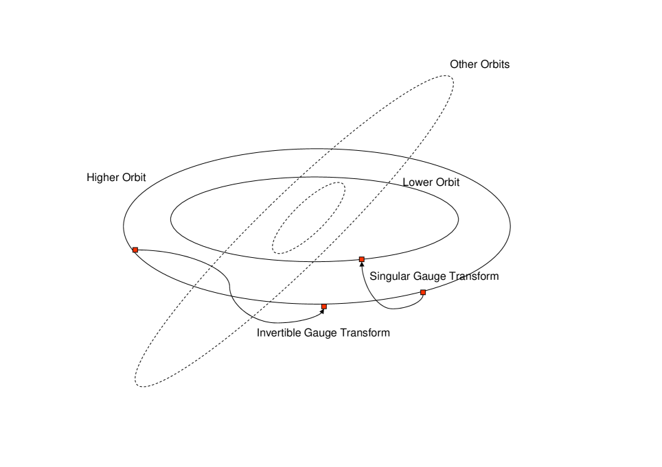
Figure 1: Gauge Transforms

Definition 17.

A gauge $(D,P)$ with term structure $P=(P_{t,s})_{t,s}$ satisfies the positive interest condition if and only if for all $t$ the function $s\mapsto P_{ts}$ is strictly monotone decreasing. Such a gauge is said to be positive. A gauge not satisfying this property is termed principal gauge. The term structure can be written as a functional of the instantaneous forward rate f defined as

$$\boxed{f_{t,s}:=-\frac{\partial}{\partial s}\log P_{t,s},\quad P_{t,s}=\exp\left(-\int_{t}^{s}dhf_{t,h}\right).}$$ (16)

and

$$\boxed{r_{t}:=\lim_{s\rightarrow t^{+}}f_{t,s}}$$ (17)

is termed short rate.

Remark 18.

Since $(P_{t,s})_{t,s}$ is a $t$-stochastic process (semimartingale) depending on a parameter $s\geq t$, the $s$-derivative can be defined deterministically, and the expressions above make sense pathwise in a both classical and generalized sense. In a generalized sense we will always have a $\mathcal{D}^{\prime}$ derivative for any $\omega\in\Omega$; this corresponds to a classic $s$-continuous derivative if $P_{t,s}(\omega)$ is a $C^{1}$-function of $s$ for any fixed $t\geq 0$ and $\omega\in\Omega$.

We see that the positive interest condition is satisfied if and only if $f_{t,s}>0$ for all $t,s$, $s\geq t$. The positive interest condition is associated with the storage requirement. Whenever it is always more valuable to get a piece of a financial object today than in the future, then it should be modelled with a gauge satisfying the positive interest condition. Examples are: non perishable goods, currencies, price indices for equities and real estates, total return indices. Examples of financial quantities not satisfying the positive interest condition and thus reflecting items which are not storable, are: inflation indices, short rates, dividend indices for equities, rental indices for real estates.

Definition 19.

The cash flow intensity $[-1]:=\delta^{\prime}$, first derivative of the Dirac delta generalized function, defines the short rate transform,

$$\begin{split}D_{t}^{[-1]}&=D_{t}\int_{0}^{+\infty}dh\,\delta^{\prime}_{h}P_{t,t+h}=D_{t}r_{t}\\ P_{t,s}^{[-1]}&=\frac{\int_{0}^{+\infty}dh\,\delta^{\prime}_{h}P_{t,s+h}}{\int_{0}^{+\infty}dh\,\delta^{\prime}_{h}P_{t,t+h}}=\frac{f_{t,s}}{r_{t}}P_{t,s}\end{split}$$ (18)

while the cash flow intensity $[+1]:=\Theta$, Heavyside function, defines the perpetuity transform

$$\begin{split}D_{t}^{[+1]}&=D_{t}\int_{0}^{+\infty}dh\,P_{t,t+h}\\ P_{t,s}^{[+1]}&=\frac{\int_{0}^{+\infty}dh\,P_{t,s+h}}{\int_{0}^{+\infty}dh\,P_{t,t+h}}.\end{split}$$ (19)

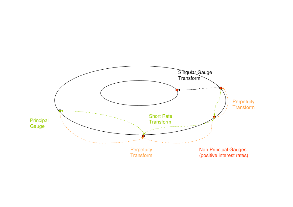
Figure 2: Short Rate and Perpetuity Transforms

Notation 20.

Repeated application of perpetuity and short rate transforms are given by:

$$\begin{split}[0]:&=\delta\text{: Dirac delta generalized function}\\ [+1]:&=\Theta\text{: Heavyside function}\\ [+k]_{t}:&=\frac{t^{k-1}}{(k-1)!}\quad(k\geq 2)\\ [-1]_{t}:&=\delta^{\prime}\text{: first derivative of Dirac delta}\\ [-k]_{t}:&=\delta^{(k)}\text{: k-th derivative of Dirac delta,}\,(k\geq 2)\end{split}$$ (20)

Thereby, for any integers $m,n$ one has $[k]\ast[l]=[k+l]$ (cf. [Hö03] Chapter IV).

The short rate and the perpetuity transform are inverse to another, as one can see from Proposition 15 and $[+1]\ast[-1]=[0]$. The short rate transform can be applied only to a positive gauge producing a gauge which possibly does not satisfy the positive interest rate condition. The perpetuity transform is a gauge transform that can be applied to any gauge producing always a positive gauge.

Proposition 21.

A gauge satisfies the positive interest condition if and only if it can be obtained as the perpetuity transform of some other gauge.

The positive interest condition is difficult to satisfy for a stochastic model of a gauge.

Example 22.

Fixed Income, Equity and Real Estate Gauges

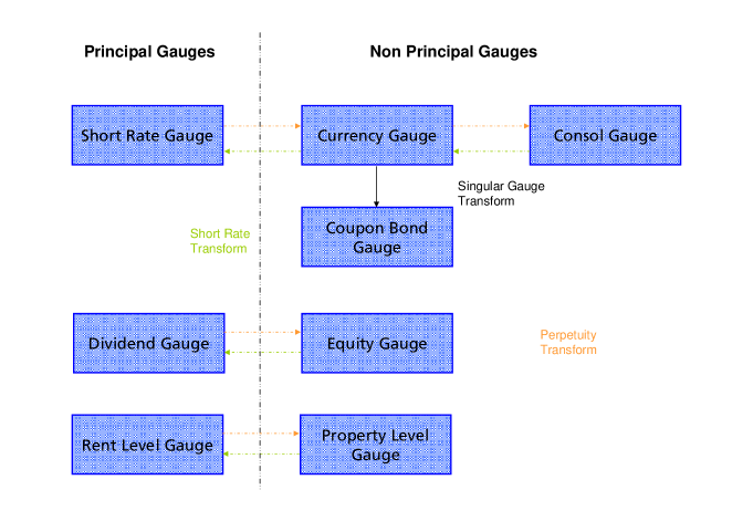
Figure 3: Gauges

Remark 23.

The special choice of vanishing interest rate $r\equiv 0$ or flat term structure $P\equiv 1$ for all assets corresponds to the classical model, where only asset prices and their dynamics are relevant. We will analyze this case in detail in the guiding example presented in section 4.

3 Arbitrage Theory in a Differential Geometric Framework

Now we are in the position to rephrase the asset model presented in subsection 2.1 in terms of a natural geometric language. That for, we will unify Smith’s and Ilinski’s ideas to model a simple market of $N$ base assets. In Smith and Speed ([SmSp98]) there is no explicit differential geometric modelling but the use of an allusive terminology (e.g. gauges, gauge transforms). In Ilinski ([Il01]) there is a construction of a principal fibre bundle allowing to express arbitrage in terms of curvature. Our construction of the principal fibre bundle will differ from Ilinski’s one in the choice of the group action and the bundle covering the base space. Our choice encodes Smith’s intuition in differential geometric language.

In this paper we explicitly model no derivatives of the base assets, that is, if derivative products have to be considered, then they have to be added to the set of base assets. The treatment of derivatives of base assets is tackled in ([FaVa12]). Given $N$ base assets we want to construct a portfolio theory and study arbitrage. Since arbitrage is explicitly allowed, we cannot a priori assume the existence of a risk neutral measure or of a state price deflator. In terms of differential geometry, we will adopt the mathematician’s and not the physicist’s approach. The market model is seen as a principal fibre bundle of the (deflator, term structure) pairs, discounting and foreign exchange as a parallel transport, numéraire as global section of the gauge bundle, arbitrage as curvature. The Ambrose-Singer Theorem allows to parameterize arbitrage strategies as element of the Lie algebra of the holonomy group. The no-free-lunch-with-vanishing-risk condition is proved to be equivalent to a zero curvature condition or to a continuity equation allowing for an hydrodynamics study of arbitrage flows.

3.1 Market Model as Principal Fibre Bundle

As a concise general reference for principle fibre bundles we refer to Bleecker’s book ([Bl81]). More extensive treatments can be found in Dubrovin, Fomenko and Novikov ([DuFoNo84]), and in the classical Kobayashi and Nomizu ([KoNo96]). Let us consider -in continuous time- a market with $N$ assets and a numéraire. A general portfolio at time $t$ is described by the vector of nominals $x\in X$, for an open set $X\subset\mathbf{R}^{N}$. Following Definition 7, the asset model induces for $j=1,\dots,N$ the gauge

$$(D^{j},P^{j})=((D_{t}^{j})_{t\in[0,+\infty[},(P_{t,s}^{j})_{s\geq t}),$$ (21)

where $D^{j}$ denotes the deflator and $P^{j}$ the term structure. This can be written as

$$P_{t,s}^{j}=\exp\left(-\int_{t}^{s}f^{j}_{t,u}du\right),$$ (22)

where $f^{j}$ is the instantaneous forward rate process for the $j$-th asset and the corresponding short rate is given by $r_{t}^{j}:=\lim_{u\rightarrow 0^{+}}f^{j}_{t,u}$. For a portfolio with nominals $x\in X\subset\mathbf{R}^{N}$ we define

$$\boxed{D_{t}^{x}:=\sum_{j=1}^{N}x_{j}D_{t}^{j}\quad f_{t,u}^{x}:=\sum_{j=1}^{N}\frac{x_{j}D_{t}^{j}}{\sum_{j=1}^{N}x_{j}D_{t}^{j}}f_{t,u}^{j}\quad P_{t,s}^{x}:=\exp\left(-\int_{t}^{s}f^{x}_{t,u}du\right).}$$ (23)

The short rate writes

$$r_{t}^{x}:=\lim_{u\rightarrow t^{+}}f^{x}_{t,u}=\sum_{j=1}^{N}\frac{x_{j}D_{t}^{j}}{\sum_{j=1}^{N}x_{j}D_{t}^{j}}r_{t}^{j}.$$ (24)

The image space of all possible strategies reads

$$\boxed{M:=\{(x,t)\in X\times[0,+\infty[\}.}$$ (25)

In subsection 2.3 cashflow intensities and the corresponding gauge transforms were introduced. They have the structure of an Abelian semigroup

$$\boxed{G:=\mathcal{E}^{\prime}([0,+\infty[,\mathbf{R})=\{F\in\mathcal{D}^{\prime}([0,+\infty[)\mid\text{supp}(F)\subset[0,+\infty[\text{ is compact}\},}$$ (26)

where the semigroup operation on distributions with compact support is the convolution (see [Hö03], Chapter IV), which extends the convolution of regular functions as defined by formula (15).

Definition 24.

The Market Fibre Bundle is defined as the fibre bundle of gauges

$$\boxed{\mathcal{B}:=\{({{D^{\pi}}_{t}}^{x},{{P^{\pi}}_{t,\,\cdot}}^{x})|(x,t)\in M,\pi\in G^{*}\}.}$$ (27)

The cashflow intensities defining invertible transforms constitute an Abelian group

$$\boxed{G^{*}:=\{\pi\in G|\text{ it exists }\nu\in G\text{ such that }\pi\ast\nu=[0]\}\subset\mathcal{E}^{\prime}([0,+\infty[,\mathbf{R}).}$$ (28)

From Proposition 15 we obtain

Theorem 25.

The market fibre bundle $\mathcal{B}$ has the structure of a $G^{*}$-principal fibre bundle given by the action

$$\begin{split}\mathcal{B}\times G^{*}&\longrightarrow\mathcal{B}\\ ((D,P),\pi)&\mapsto(D,P)^{\pi}=(D^{\pi},P^{\pi}).\end{split}$$ (29)

The group $G^{*}$ acts freely and differentiably on $\mathcal{B}$ to the right.

3.2 Numéraire as Global Section of the Bundle of Gauges

If we want to make an arbitrary portfolio of the given assets specified by the nominal vector $x^{\text{Num}}$ to our numéraire, we have to renormalize all deflators by an appropriate gauge transform $\pi^{\text{Num},x}$ so that:

• The portfolio value is constantly over time normalized to one:

  $$D_{t}^{x^{\text{Num}},\pi^{\text{Num}}}\equiv 1.$$ (30)

• All other assets’ and portfolios’ are expressed in terms of the numéraire:

  $$D_{t}^{x,\pi^{\text{Num}}}=\text{FX}_{t}^{x\rightarrow x^{\text{Num}}}:=\frac{D^{x}_{t}}{D^{x^{\text{Num}}}_{t}}.$$ (31)

It is easily seen that the appropriate choice for the gauge transform $\pi^{\text{Num}}$ making the portfolio $x^{\text{Num}}$ to the numéraire is given by the global section of the bundle of gauges defined by

$$\boxed{\pi^{\text{Num},x}_{t}:=\text{FX}_{t}^{x\rightarrow x^{\text{Num}}}.}$$ (32)

Of course such a gauge transform is well defined if and only if the numéraire deflator is a positive semimartingale.

3.3 Cashflows as Sections of the Associated Vector Bundle

By choosing the fiber $V:=\mathbf{R}^{[0,+\infty[}$ and the representation $\rho:G\rightarrow\text{GL}(V)$ induced by the gauge transform definition, and therefore satisfying the homomorphism relation $\rho(g_{1}\ast g_{2})=\rho(g_{1})\rho(g_{2})$, we obtain the associated vector bundle $\mathcal{V}$. Its sections represents cashflow streams - expressed in terms of the deflators - generated by portfolios of the base assets. If $v=(v^{x}_{t})_{(x,t)\in M}$ is the deterministic cashflow stream, then its value at time $t$ is equal to

• the deterministic quantity $v_{t}^{x}$, if the value is measured in terms of the deflator $D_{t}^{x}$,

• the stochastic quantity $v^{x}_{t}D^{x}_{t}$, if the value is measured in terms of the numéraire (e.g. the cash account for the choice $D_{t}^{j}:=\hat{S}_{t}^{j}$ for all $j=1,\dots,N$).

In the general theory of principal fibre bundles, gauge transforms are bundle automorphisms preserving the group action and equal to the identity on the base space. Gauge transforms of $\mathcal{B}$ are naturally isomorphic to the sections of the bundle $\mathcal{B}$ (See Theorem 3.2.2 in [Bl81]). Since $G^{*}$ is Abelian, right multiplications are gauge transforms. Hence, there is a bijective correspondence between gauge transforms and cashflow intensities admitting an inverse. This justifies the terminology introduced in Definition 12.

3.4 Derivatives of Stochastic Processes

One of the main contribution of this paper is to reformulate stochastic finance in a natural geometric language. In stochastic differential geometry one would like to lift the constructions of stochastic analysis from open subsets of $\mathbf{R}^{N}$ to $N$ dimensional differentiable manifolds. To that aim, chart invariant definitions are needed and hence a stochastic calculus satisfying the usual chain rule and not Itô’s Lemma is required. (cf. [HaTh94], Chapter 7, and the remark in Chapter 4 at the beginning of page 200). That is why we will be mainly concerned in the following by stochastic integrals and derivatives meant in the sense of Stratonovich and not of Itô. Following [Gl11] and [CrDa07] we introduce the following

Definition 26.

Let $I$ be a real interval and $Q=(Q_{t})_{t\in I}$ be a vector valued stochastic process on the probability space $(\Omega,\mathcal{A},P)$. The process $Q$ determines three families of $\sigma$-subalgebras of the $\sigma$-algebra $\mathcal{A}$:

• ”Past” $\mathcal{P}_{t}$, generated by the preimages of Borel sets in $\mathbf{R}^{N}$ by all mappings $Q_{s}:\Omega\rightarrow\mathbf{R}^{N}$ for $0<s<t$.

• ”Future” $\mathcal{F}_{t}$, generated by the preimages of Borel sets in $\mathbf{R}^{N}$ by all mappings $Q_{s}:\Omega\rightarrow\mathbf{R}^{N}$ for $0<t<s$.

• ”Present” $\mathcal{N}_{t}$, generated by the preimages of Borel sets in $\mathbf{R}^{N}$ by the mapping $Q_{t}:\Omega\rightarrow\mathbf{R}^{N}$.

Let $Q=(Q_{t})_{t\in I}$ be a $\mathcal{S}^{0}(I)$-process, i.e. a process with continuous sample paths and adapted to $\mathcal{P}$ and $\mathcal{F}$, so that $t\mapsto Q_{t}$ is a continuous mapping continuous mappings from $I$ to $L^{2}(\Omega,\mathcal{A})$. Assuming that the following limits exist, Nelson’s stochastic derivatives are defined as

$$\boxed{\begin{split}&\mathfrak{D}Q_{t}:=\lim_{h\rightarrow 0^{+}}\mathbb{E}\left[\left.\frac{Q_{t+h}-Q_{t}}{h}\right|\mathcal{P}_{t}\right]\text{: forward derivative,}\\ &\mathfrak{D}_{*}Q_{t}:=\lim_{h\rightarrow 0^{+}}\mathbb{E}\left[\left.\frac{Q_{t}-Q_{t-h}}{h}\right|\mathcal{F}_{t}\right]\text{: backward derivative,}\\ &\mathcal{D}Q_{t}:=\frac{\mathfrak{D}Q_{t}+\mathfrak{D}_{*}Q_{t}}{2}\text{: mean derivative}.\end{split}}$$ (33)

Let $\mathcal{S}^{1}(I)$ the set of all $\mathcal{S}^{0}(I)$-processes $Q$ such that $t\mapsto\mathfrak{D}Q_{t}$ and $t\mapsto\mathfrak{D}_{*}Q_{t}$ are continuous mappings from $I$ to $L^{2}(\Omega,\mathcal{A})$. Let $\mathcal{C}^{1}(I)$ the completion of $\mathcal{S}^{1}(I)$ with respect to the norm

$$\|Q\|:=\sup_{t\in I}\left(\|Q_{t}\|_{L^{2}(\Omega,\mathcal{A})}+\|\mathfrak{D}Q_{t}\|_{L^{2}(\Omega,\mathcal{A})}+\|\mathfrak{D}_{*}Q_{t}\|_{L^{2}(\Omega,\mathcal{A})}\right).$$ (34)

Remark 27.

The stochastic derivatives $\mathfrak{D}$, $\mathfrak{D}_{*}$ and $\mathcal{D}$ correspond to Itô’s, to the anticipative and, respectively, to Stratonovich’s integral (cf. [Gl11]). The process space $\mathcal{C}^{1}(I)$ contains all Itô processes. If $Q$ is a Markov process, then the sigma algebras $\mathcal{P}_{t}$ (”past”) and $\mathcal{F}_{t}$ (”future”) in the definitions of forward and backward derivatives can be substituted by the sigma algebra $\mathcal{N}_{t}$ (”present”), see Chapter 6.1 and 8.1 in ([Gl11]).

Stochastic derivatives can be defined pointwise in $\omega\in\Omega$ outside the class $\mathcal{C}^{1}$ in terms of generalized functions.

Definition 28.

Let $Q:I\times\Omega\rightarrow\mathbb{R}^{N}$ be a continuous linear functional in the test processes $\varphi:I\times\Omega\rightarrow\mathbb{R}^{N}$ for $\varphi(\cdot,\omega)\in C^{\infty}_{c}(I,\mathbb{R}^{N})$. We mean by this that for a fixed $\omega\in\Omega$ the functional $Q(\cdot,\omega)\in\mathcal{D}(I,\mathbb{R}^{N})$, the topological vector space of continuous distributions. We can then define Nelson’s generalized stochastic derivatives:

$$\boxed{\begin{split}&\mathfrak{D}Q(\varphi_{t}):=-Q(\mathfrak{D}\varphi_{t})\text{: forward generalized derivative,}\\ &\mathfrak{D}_{*}Q(\varphi_{t}):=-Q(\mathfrak{D}_{*}\varphi_{t})\text{: backward generalized derivative,}\\ &\mathcal{D}(\varphi_{t}):=-Q(\mathcal{D}\varphi_{t})\text{: mean generalized derivative}.\end{split}}$$ (35)

If the generalized derivative is regular, then the process has a derivative in the classic sense. This construction is nothing else than a straightforward pathwise lift of the theory of generalized functions to a wider class stochastic processes which do not a priori allow for Nelson’s derivatives in the strong sense. We will utilize this feature in the treatment of credit risk, where many processes with jumps occur.

3.5 Stochastic Parallel Transport and Holonomy

Let us consider the projection of $\mathcal{B}$ onto $M$

$$\begin{split}p:\mathcal{B}\cong M\times G^{*}&\longrightarrow M\\ (x,t,g)&\mapsto(x,t)\end{split}$$ (36)

and its tangential map

$$T_{(x,t,g)}p:\underbrace{T_{(x,t,g)}\mathcal{B}}_{\cong\mathbf{R}^{N}\times\mathbf{R}\times\mathbf{R}^{[0,+\infty[}}\longrightarrow\underbrace{T_{(x,t)}M}_{\cong\mathbf{R}^{N}\times\mathbf{R}.}$$ (37)

The vertical directions are

$$\mathcal{V}_{(x,t,g)}\mathcal{B}:=\ker\left(T_{(x,t,g)}p\right)\cong\mathbf{R}^{[0,+\infty[},$$ (38)

and the horizontal ones are

$$\mathcal{H}_{(x,t,g)}\mathcal{B}\cong\mathbf{R}^{N+1}.$$ (39)

A connection on $\mathcal{B}$ is a projection $T\mathcal{B}\rightarrow\mathcal{V}\mathcal{B}$. More precisely, the vertical projection must have the form

$$\begin{split}\Pi^{v}_{(x,t,g)}:T_{(x,t,g)}\mathcal{B}&\longrightarrow\mathcal{V}_{(x,t,g)}\mathcal{B}\\ (\delta x,\delta t,\delta g)&\mapsto(0,0,\delta g+\Gamma(x,t,g).(\delta x,\delta t)),\end{split}$$ (40)

and the horizontal one must read

$$\begin{split}\Pi^{h}_{(x,t,g)}:T_{(x,t,g)}\mathcal{B}&\longrightarrow\mathcal{H}_{(x,t,g)}\mathcal{B}\\ (\delta x,\delta t,\delta g)&\mapsto(\delta x,\delta t,-\Gamma(x,t,g).(\delta x,\delta t)),\end{split}$$ (41)

such that

$$\Pi^{v}+\Pi^{h}=\mathbf{1}_{\mathcal{B}}.$$ (42)

Stochastic parallel transport on a principal fibre bundle along a semimartingale is a well defined construction (cf. [HaTh94], Chapter 7.4 and [Hs02] Chapter 2.3 for the frame bundle case) in terms of Stratonovich’s integral. Existence and uniqueness can be proved analogously to the deterministic case by formally substituting the deterministic time derivative $\frac{d}{dt}$ with the stochastic one $\mathcal{D}$ corresponding to Stratonovich’s integral.

Following Ilinski’s idea ([Il01]), we motivate the choice of a particular connection by the fact that it allows to encode foreign exchange and discounting as parallel transport.

Theorem 29.

With the choice of connection

$$\boxed{\Gamma(x,t,g).(\delta x,\delta t):=g\left(\frac{D_{t}^{\delta x}}{D_{t}^{x}}-r_{t}^{x}\delta t\right),}$$ (43)

the parallel transport in $\mathcal{B}$ has the following financial interpretations:

• Parallel transport along the nominal directions ($x$-lines) corresponds to a multiplication by an exchange rate.

• Parallel transport along the time direction ($t$-line) corresponds to a division by a stochastic discount factor.

Recall that time derivatives needed to define the parallel transport along the time lines have to be understood in Stratonovich’s sense. We see that the bundle is trivial, because it has a global trivialization, but the connection is not trivial.

Proof.

Let us consider a curve $\gamma(\tau)=(x(\tau),t(\tau))$ in $M$ for $\tau\in[\tau_{1},\tau_{2}]$ and an element of the fiber over the starting point $g_{1}\in p^{-1}(\gamma(\tau_{1}))\cong G$. The parallel transport of $g_{1}$ along $\gamma$ is the solution $g=g(\tau)$ of the first order differential equation

$$\begin{cases}\Pi^{v}_{(x(\tau),t(\tau),g(\tau))}(\mathcal{D}x(\tau),\mathcal{D}t(\tau),\mathcal{D}g(\tau))=0\\ g(\tau_{1})=g_{1},\end{cases}$$ (44)

which in our case writes

$$\begin{cases}\mathcal{D}g(\tau)=-g(\tau)\left(\frac{D_{t(\tau)}^{\mathcal{D}x(\tau)}}{D_{t(\tau)}^{x(\tau)}}-r_{t(\tau)}^{x(\tau)}\mathcal{D}t(\tau)\right)\\ g(\tau_{1})=g_{1},\end{cases}$$ (45)

Recall that the time derivative $\mathcal{D}$ is Nelson’s derivative corresponding to Stratonovich’s integral, see subsection 3.4. Now, if $\gamma$ is a nominal direction, then $t(\tau)\equiv t$ and $\mathcal{D}t(\tau)\equiv 0$. Thus

$$\begin{cases}\mathcal{D}g(\tau)=-g(\tau)\frac{\sum_{j=1}^{N}\mathcal{D}x_{j}(\tau)D_{t}^{j}}{\sum_{j=1}^{N}x_{j}(\tau)D_{t}^{j}}\\ g(\tau_{1})=g_{1},\end{cases}$$ (46)

which means

$$g(\tau)=g_{1}\frac{\sum_{j=1}^{N}x_{j}(\tau_{1})D_{t}^{j}}{\sum_{j=1}^{N}x_{j}(\tau)D_{t}^{j}}$$ (47)

corresponding to a multiplication by an exchange rate at time $t$ from portfolio $x(\tau_{1})$ to portfolio $x(\tau)$.
If $\gamma$ is the time direction, then $x(\tau)\equiv x$, $t(\tau)=\tau$ and $\mathcal{D}x(\tau)\equiv 0$, $\mathcal{D}t(\tau)\equiv 1$ . Thus

$$\begin{cases}\mathcal{D}g(\tau)=g(\tau)r_{\tau}^{x}\\ g(\tau_{1})=g_{1},\end{cases}$$ (48)

which means

$$g(\tau)=g_{1}\exp\left(\int_{\tau_{1}}^{\tau}r^{x}_{u}du\right)$$ (49)

corresponding to a division by the stochastic discount rate for portfolio $x$ from time $\tau_{1}$ to time $\tau$. ∎

Remark 30.

Malaney and Weinstein ([Ma96]) already introduced a connection in the deterministic case in the context of self-financing basket of goods for divisa indices. Recently, [FaVa12] have elaborated a stochastic version of the Malaney-Weinstein connection proving its equivalence with the connection defined in (43).

Holonomy is the group generated by the parallel transport along closed curves. We distinguish the local from the global case.

Definition 31.

The holonomy group based at $b\in\mathcal{B}$ is defined as

$$\boxed{\operatorname{Hol}_{b}(\chi):=\{g\in G\mid\,b\text{ and }b.g\text{ can be joined by an horizontal curve in }\mathcal{B}\}.}$$ (50)

The local holonomy group based at $b\in\mathcal{B}$ is defined as

$$\boxed{\begin{split}\operatorname{Hol}_{b}^{0}(\chi):=&\left\{g\in G\mid\,b\text{ and }b.g\text{ can be joined by a contractible horizontal}\right.\\ &\left.\text{ curve in }\mathcal{B}\right\}.\end{split}}$$ (51)

If $M$ and $\mathcal{B}$ are connected, then holonomy and local holonomy depend on the base point $b$ only up to conjugation. In this paper we will always assume connectivity for both $M$ and $\mathcal{B}$ and therefore drop the reference to the basis point $b$, with the understanding that the definition is good up to conjugation.

3.6 Nelson $\mathcal{D}$ Differentiable Market Model

We continue to reformulate the classic asset model introduced in subsection 2.1 in terms of stochastic differential geometry.

Definition 32.

A Nelson $\mathcal{D}$ weak differentiable market model for $N$ assets is described by $N$ gauges which are Nelson $\mathcal{D}$ weak differentiable with respect to the time variable. More exactly, for all $t\in[0,+\infty[$ and $s\geq t$ there is an open time interval $I\ni t$ such that for the deflators $D_{t}:=[D_{t}^{1},\dots,D_{t}^{N}]^{\dagger}$ and the term structures $P_{t,s}:=[P_{t,s}^{1},\dots,P_{t,s}^{N}]^{\dagger}$, the latter seen as processes in $t$ and parameter $s$, there exist a $\mathcal{D}$ weak $t$-derivative. The short rates are defined by $r_{t}:=\lim_{s\rightarrow t^{+}}-\frac{\partial}{\partial s}\log P_{ts}$.

A strategy is a curve $\gamma:I\rightarrow X$ in the portfolio space parameterized by the time. This means that the allocation at time $t$ is given by the vector of nominals $x_{t}:=\gamma(t)$. We denote by $\bar{\gamma}$ the lift of $\gamma$ to $M$, that is $\bar{\gamma}(t):=(\gamma(t),t)$. A strategy is said to be closed if it represented by a closed curve. A weak $\mathcal{D}$-admissible strategy is predictable and $\mathcal{D}$- weak differentiable.

In general the allocation can depend on the state of the nature i.e. $x_{t}=x_{t}(\omega)$ for $\omega\in\Omega$. Unless otherwise specified strategies will always be weak $\mathcal{D}$-admissible for an appropriate time interval.

Proposition 33.

A weak $\mathcal{D}$-admissible strategy is self-financing if and only if

$$\mathcal{D}(x_{t}\cdot D_{t})=x_{t}\cdot\mathcal{D}D_{t}-\frac{1}{2}\mathfrak{D}_{*}\left<x,D\right>_{t}\quad\text{or}\qquad\mathcal{D}x_{t}\cdot D_{t}=-\frac{1}{2}\mathfrak{D}_{*}\left<x,D\right>_{t},$$ (52)

almost surely.

Proof.

The strategy is self-financing if and only if

$$x_{t}\cdot D_{t}=x_{0}\cdot D_{0}+\int_{0}^{t}x_{u}\cdot dD_{u},$$ (53)

which is, symbolizing $d$ Itô’s ”differential”, equivalent to

$$\mathfrak{D}(x_{t}\cdot D_{t})=x_{t}\cdot\mathfrak{D}D_{t}.$$ (54)

The selfinancing condition can be expressed by means of the anticipative ”differential” $d_{*}$ as

$$x_{t}\cdot D_{t}=x_{0}\cdot D_{0}+\int_{0}^{t}x_{u}\cdot d_{*}D_{u}-\int_{0}^{t}d\left<x,D\right>_{u},$$ (55)

which is equivalent to

$$\mathfrak{D}_{*}(x_{t}\cdot D_{t})=x_{t}\cdot\mathfrak{D}_{*}D_{t}-\mathfrak{D}_{*}\left<x,D\right>_{t}.$$ (56)

By summing equations (54) and (56) we obtain

$$\mathcal{D}(x_{t}\cdot D_{t})=\frac{1}{2}(\mathfrak{D}+\mathfrak{D}_{*})(x_{t}\cdot D_{t})=x_{t}\cdot\mathcal{D}D_{t}-\frac{1}{2}\mathfrak{D}_{*}\left<x,D\right>_{t}.$$ (57)

To prove the second statement in expression 52 we consider the integration by part formula for Itô’s integral

$$\int_{0}^{t}x_{u}\cdot dD_{u}+\int_{0}^{t}D_{u}\cdot dx_{u}=x_{t}\cdot D_{t}-x_{0}\cdot D_{0}-\left<x,D\right>_{t},$$ (58)

which, expressed in terms of Stratonovich’s integral, leads to

$$\int_{0}^{t}x_{u}\circ dD_{u}-\frac{1}{2}\left<x,D\right>_{t}+\int_{0}^{t}D_{u}\circ dx_{u}-\frac{1}{2}\left<x,D\right>_{t}=x_{t}\cdot D_{t}-x_{0}\cdot D_{0}-\left<x,D\right>_{t}.$$ (59)

By taking Stratonovich’s derivative $\mathcal{D}$ on both side we get

$$\mathcal{D}(x_{t}\cdot D_{t})=\mathcal{D}x_{t}\cdot D_{t}+x_{t}\cdot\mathcal{D}D_{t},$$ (60)

which, together with the first statement in expression (52) proves the second one. ∎

For the reminder of this paper unless otherwise stated we will deal only with weak $\mathcal{D}$ differentiable market models, weak $\mathcal{D}$ differentiable strategies, and, when necessary, with weak $\mathcal{D}$ differentiable state price deflators. All Itô processes are weak $\mathcal{D}$ differentiable, so that the class of considered admissible strategies is very large.

3.7 Arbitrage as Curvature

The Lie algebra of $G$ is

$$\mathfrak{g}=\mathbf{R}^{[0,+\infty[}$$ (61)

and therefore commutative. The $\mathfrak{g}$-valued connection $1$-form writes as

$$\chi(x,t,g)(\delta x,\delta t)=\left(\frac{D_{t}^{\delta x}}{D_{t}^{x}}-r_{t}^{x}\delta t\right)g,$$ (62)

or as a linear combination of basis differential forms as

$$\boxed{\chi(x,t,g)=\left(\frac{1}{D_{t}^{x}}\sum_{j=1}^{N}D_{t}^{j}dx_{j}-r_{t}^{x}dt\right)g.}$$ (63)

The $\mathfrak{g}$-valued curvature $2$-form is defined as

$$R:=d\chi+[\chi,\chi],$$ (64)

meaning by this, that for all $(x,t,g)\in\mathcal{B}$ and for all $\xi,\eta\in T_{(x,t)}M$

$$R(x,t,g)(\xi,\eta):=d\chi(x,t,g)(\xi,\eta)+[\chi(x,t,g)(\xi),\chi(x,t,g)(\eta)].$$ (65)

Remark that, being the Lie algebra commutative, the Lie bracket $[\cdot,\cdot]$ vanishes. After some calculations we obtain

$$\boxed{R(x,t,g)=\frac{g}{D_{t}^{x}}\sum_{j=1}^{N}D_{t}^{j}\left(r_{t}^{x}+\mathcal{D}\log(D_{t}^{x})-r_{t}^{j}-\mathcal{D}\log(D_{t}^{j})\right)dx_{j}\wedge dt,}$$ (66)

and can prove following results which characterizes arbitrage as curvature.

Theorem 34 (No Arbitrage).

The following assertions are equivalent:

• The market model satisfies the no-free-lunch-with-vanishing-risk condition.

• There exists a positive martingale $\beta=(\beta_{t})_{t}$ such that deflators and short rates satisfy for all portfolio nominals and all times the condition

  $$\boxed{r_{t}^{x}=-\mathcal{D}\log(\beta_{t}D_{t}^{x}).}$$ (67)

• There exists a positive martingale $\beta=(\beta_{t})_{t}$ such that deflators and term structures satisfy for all portfolio nominals and all times the condition

  $$\boxed{P^{x}_{t,s}=\frac{\mathbb{E}_{t}[\beta_{s}D^{x}_{s}]}{\beta_{t}D^{x}_{t}}.}$$ (68)

The following assertions are equivalent and follow from the above ones:

• The local holonomy group $\operatorname{Hol}^{0}(\chi)$ of the principal fibre bundle $\mathcal{B}$ is trivial.

• The curvature form $R$ vanishes everywhere on $\mathcal{B}$.

Proof.

• (i)$\Leftrightarrow$(iii): By Theorems 2 and 4 the no-free-lunch-with-vanishing-risk property is equivalent to the existence of a positive state price deflator, that is of a positive martingale $\beta=(\beta_{t})_{t}$ such that the market value at time $t$ of the any contingent claim at time $s>t$ of the form $D_{s}^{x}$ is

  $$\frac{1}{\beta_{t}}\mathbb{E}_{t}[\beta_{s}D_{s}^{x}],$$ (69)

  where $\mathbb{E}_{t}$ denotes conditional expectation. Since prices are expressed in units of the deflator to which they relate the formula writes

  $$D_{t}^{x}P_{t,s}^{x}=\frac{1}{\beta_{t}}\mathbb{E}_{t}[\beta_{s}D_{s}^{x}].$$ (70)

• (ii)$\Leftrightarrow$(iii): the first equation is the integral version of the second, which is the differential version of the first. This can be seen by the following reasoning. Differentiating equation (68) with respect to $\mathcal{D}_{s}$ on both sides leads to

  $$D^{x}_{t}\exp\left(\int_{t}^{s}f^{x}_{t,u}du\right)(-f_{t,s}^{x})=\frac{1}{\beta_{t}}\mathcal{D}_{s}\mathbb{E}_{t}[\beta_{s}D_{s}^{x}].$$ (71)

  By taking the limit for $s\rightarrow t^{+}$ on both sides, one obtains, by continuity,

  $$-D_{t}^{x}r_{t}^{x}=\frac{1}{\beta_{t}}\mathcal{D}_{t}(\beta_{t}D_{t}^{x}),$$ (72)

  which is equation (67). This proves the implication $(ii)\Rightarrow(iii)$.
  If we integrate (67), we obtain

  $$-\int_{t}^{s}du\,r_{u}^{x}=\log\left(\frac{\beta_{s}D_{s}^{x}}{\beta_{t}D_{t}^{x}}\right),$$ (73)

  which means

  $$D^{x}_{t}\exp\left(-\int_{t}^{s}du\,r_{u}^{x}\right)=\frac{1}{\beta_{t}}\beta_{s}D_{s}^{x}.$$ (74)

  Taking the conditional expectation $\mathbb{E}_{t}[\cdot]$ on both sides leads to

  $$D^{x}_{t}\mathbb{E}_{t}\left[\exp\left(-\int_{t}^{s}du\,r_{u}^{x}\right)\right]=\frac{1}{\beta_{t}}\mathbb{E}_{t}[\beta_{s}D_{s}^{x}],$$ (75)

  which is equivalent to equation(68). Therefore, the implication $(iii)\Rightarrow(ii)$ is proved.

• (ii)$\Rightarrow$(v):

  $$\mathcal{D}\log(D_{t}^{x})+r_{t}^{x}=-\mathcal{D}\log\beta_{t}=:\text{Const}_{t}\Rightarrow R\equiv 0,$$ (76)

  where $\text{Const}_{t}$ depends only on the time $t$ but not on the portfolio $x$.

• (iv)$\Leftrightarrow$(v): The bundle is trivial. The assertion is then a standard result in differential geometry (the Ambrose-Singer Theorem), see f.i. [KoNo96] Chapters II.4 and II.8.

∎

The preceding Theorem motivates the following definition

Definition 35.

The market model satisfies the zero curvature condition (ZC) if and only if the curvature vanishes a.s.

Therefore, we have following implications relying the three different definitions of no-arbitrage:

Corollary 36.

$$\boxed{\begin{split}&\text{(NFLVR)}\Rightarrow\text{(NA)}\\ &\text{(NFLVR)}\Rightarrow\text{(ZC)}\end{split}}$$ (77)

Proof.

The first implication is well known in mathematical finance (see Definition 1). That (NFLVR) implies (ZC) is a consequence of Theorem 34. ∎

3.8 No Arbitrage Condition, Flows and Continuity Equation

The geometric language introduced enlightens similarities between the asset model on one side and hydro- or electrodynamics on the other. The counterpart of a liquid or charge flow in physics is a value flow in mathematical finance. The associated continuity equation is satisfied if and only if the no-free-lunch-with-vanishing-risk condition is fulfilled.

Definition 37.

Let $M_{t}(x):=\{y|(y,t)\in M,\,y\leq x\}$ be the set of all possible portfolios at time $t$ bounded from above by the portfolio $y$, and $M_{t}^{j}(x)\subset]-\infty,x_{j}]$ its projection onto the $j$th axis. The log value current for the market model is defined as a vector field $J$ on $M$ by

$$\boxed{J^{j}(x,t):=\left(\int_{M_{t}^{j}(x)}dy_{j}\,\frac{y_{j}D_{t}^{j}}{D_{t}^{(y_{j}e_{j}+\sum_{i\neq j}x_{i}e_{i})}}\right)r_{t}^{j},}$$ (78)

where $r_{t}:=[r_{t}^{1},\dots,r_{t}^{N}]^{\dagger}$ and $r_{t}\,u$ the componentwise multiplication. Let $\beta=(\beta_{t})_{t}$ be a positive semimartingale. The $\beta$-scaled log value density for the market model is defined on $M$ as

$$\boxed{\rho^{\beta}(x,t):=\log(\beta_{t}D_{t}^{x}).}$$ (79)

The results of the preceding subsection can be reformulated in terms of a continuity equation analogously to classical electrodynamics (cf. [Ja98], 5.1, p. 175) or continuum mechanics (cf. [Ši02], 3.3.1, pp. 67-68).

Theorem 38 (Continuity Equation).

The market model satisfies the no-free-lunch-with-vanishing-risk-condition if and only if there exists a positive martingale $\beta$ such that one of following equations is satisfied:

$$\boxed{\begin{split}&\mathcal{D}\rho^{\beta}+\operatorname{div}_{x}J=0\\ &\mathcal{D}\int_{X_{t_{0}}}dx^{N}\rho^{\beta}=-\oint_{\partial X_{t_{0}}}dn\cdot J.\end{split}}$$ (80)

The first expression is the differential version of the continuity equation and the second the integral one, which must hold text for any $1-$codimensional submanifold $X_{t_{0}}$ lying in the hyperplane $t\equiv t_{0}$.

The integral version of the continuity equation has a beautiful financial interpretation: a market satisfies the no-free-lunch-with- vanishing-risk condition if and only if the log total value change of any submarket is due to the log value current flow through its boundary.

Proof.

It is an application of the vector field divergence definition:

$$\operatorname{div}_{x}J(x,t)=\sum_{j=1}^{N}\frac{\partial}{\partial x_{j}}J(x,t)=r_{t}^{x}=-\mathcal{D}\log(\beta_{t}D_{t}^{x}).$$ (81)

Gauss’ Theorem proves the integral version. ∎

The left hand side expression in the differential version of the continuity equation (80) is a natural candidate for a local arbitrage measure. The link with the definition of arbitrage given in the preceding section is given by

Proposition 39 (Curvature Formula).

Let $R$ be the curvature, $\rho^{\beta}$ the log value density and $J$ the log value current. Then, the following quality holds:

$$\boxed{R(x,t,g)=gdt\wedge d_{x}\left[\mathcal{D}\rho^{\beta}+\operatorname{div}_{x}J\right]=gdt\wedge d_{x}\left[\mathcal{D}\log(D_{t}^{x})+r_{t}^{x}\right].}$$ (82)

Proof.

We develop the expression for the curvature as:

$$\begin{split}R(x,t,g)&=\frac{g}{D_{t}^{x}}\sum_{j=1}^{N}D_{t}^{j}\left(r_{t}^{x}+\mathcal{D}\log(D_{t}^{x})-r_{t}^{j}-\mathcal{D}\log(D_{t}^{j})\right)dx_{j}\wedge dt=\\ &=g\sum_{j=1}^{N}\frac{\partial}{\partial x_{j}}\left(-\mathcal{D}\log(D_{t}^{x})-r_{t}^{x}\right)dx_{j}\wedge dt=\\ &=g\sum_{j=1}^{N}\frac{\partial}{\partial x_{j}}\left(-\mathcal{D}\log(\beta_{t}D_{t}^{x})-r_{t}^{x}\right)dx_{j}\wedge dt=\\ &=g\sum_{j=1}^{N}\frac{\partial}{\partial x_{j}}\left(\mathcal{D}\rho^{\beta}+\operatorname{div}_{x}(J)\right)dt\wedge dx_{j}=\\ &=gdt\wedge d_{x}\left[\mathcal{D}\rho^{\beta}+\operatorname{div}_{x}J\right]=\\ &=gdt\wedge d_{x}\left[\mathcal{D}\log(D_{t}^{x})+r_{t}^{x}\right].\end{split}$$ (83)

∎

Corollary 40 (No Arbitrage Revisited).

The following assertions are equivalent:

• The market model satisfies the no-free-lunch-with-vanishing-risk condition.

• There exist a positive martingale $\beta$ for which the continuity equation is satisfied.

4 A Guiding Example

We want now to construct an example to demonstrate how the most important geometric concepts of section 2 can be applied. Given a filtered probability space $(\Omega,\mathcal{A},P)$, where $P$ is the statistical (physical) probability measure, we assume that all processes introduced in this example are adapted to the filtration $\mathcal{A}=(\mathcal{A}_{t})_{t\in[0,+\infty[}$ satisfying the usual conditions. Let us consider a market consisting of $N+1$ assets labeled by $j=0,1,\dots,N$, where the $0$-th asset is the cash account utilized as a numéraire. Therefore, as explained in the introductory subsection 2.1, it suffices to model the price dynamics of the other assets $j=1,\dots,N$ expressed in terms of the $0$-th asset. As vector valued semimartingale for the discounted price process $\hat{S}:[0,+\infty[\times\Omega\rightarrow\mathbf{R}^{N}$, we chose the multidimensional Itô-process given by

$$d\hat{S}_{t}=\hat{S}_{t}(\alpha_{t}dt+\sigma_{t}dW_{t}),$$ (84)

where

• $(W_{t})_{t\in[0,+\infty[}$ is a standard $P$-Brownian motion in $\mathbb{R}^{K}$, for some $K\in\mathbb{N}$, and,

• $(\sigma_{t})_{t\in[0,+\infty[}$, $(\alpha_{t})_{t\in[0,+\infty[}$ are $\mathbb{R}^{N\times K}$-, and respectively, $\mathbb{R}^{N}$- valued stochastic processes, $\sigma_{t}$ as maximal rank, i.e. $\text{rank}(\sigma_{t})=K$,

The processes $\alpha$ and $\sigma$ generalize drift and volatility of a multidimensional geometric Brownian motion. Therefore, we have modelled assets satisfying the zero liability assumptions like stocks, bonds and commodities. The solution of the SDE (84) can be obtained by means of Itô’s Lemma and reads

$$\hat{S}_{t}=\hat{S}_{0}\exp\left(\int_{0}^{t}\left(\alpha_{u}-\frac{1}{2}\operatorname{diag}(\sigma_{u}\sigma_{u}^{\dagger})\right)du+\int_{0}^{t}\sigma_{u}dW_{u}\right),$$ (85)

where integration and exponentiation are meant componentwise. To define the corresponding deflators to meet Definition 7, we can just set

$$D:=\hat{S}.$$ (86)

In order to construct term structures representing future contracts on the assets, we pass by the definition of their short rates as in Definition 17, assuming that they follow the multidimensional Itô-process

$$dr_{t}=a_{t}dt+b_{t}dW_{t},$$ (87)

where $W$ is the multidimensional $P$-Brownian motion introduced above and $(b_{t})_{t\in[0,+\infty[}$, $(a_{t})_{t\in[0,+\infty[}$ are $\mathbf{R}^{N\times K}$-, and respectively, $\mathbf{R}^{N}$- valued locally bounded predictable stochastic processes, the drift and the instantaneous volatility of the multidimensional short rate. The solution of the SDE (87) writes

$$r_{t}=r_{0}+\int_{0}^{t}a_{u}du+\int_{0}^{t}b_{u}dW_{u}.$$ (88)

Term structures are defined via

$$P_{t,s}:=\mathbb{E}_{t}\left[\exp\left(-\int_{t}^{s}r_{u}du\right)\right].$$ (89)

At time $t$, the price of synthetic zero bonds delivering at time $s$ one unit of the base asset $j$ is

$$\bar{S}_{t}^{j}:=\hat{S}_{t}P^{j}_{t,s}.$$ (90)

This means that we have constructed $N$ gauges

$$(D^{j},P^{j})\quad j=1,\dots,N,$$ (91)

satisfying Definition 7. Moreover, if drifts $\alpha,a$ and volatilities $\sigma,b$ satisfy appropriate regularity assumptions, then we have a Nelson $\mathcal{D}$ differentiable market model as in Definition 32 with nominal space $X=\mathbf{R}^{N}$ and base manifold $M=\mathbf{R}^{N}\times[0,+\infty[$. The dynamics of asset prices, short rates and term structures read

$$\begin{split}\hat{S}_{t}^{x}&=x^{\dagger}\hat{S}_{0}\exp\left(\int_{0}^{t}(\alpha_{u}-\frac{1}{2}\operatorname{diag}({\sigma_{u}}\sigma_{u}^{\dagger}))du+\int_{0}^{t}\sigma_{u}dW_{u}\right)\\ r_{t}^{x}&=\frac{x^{\dagger}}{\hat{S}_{t}^{x}}\hat{S}_{t}(r_{0}+\int_{0}^{t}a_{u}du+\int_{0}^{t}b_{u}dW_{u})\\ P_{t,s}^{x}&=\mathbb{E}_{t}\left[\exp\left(-\int_{t}^{s}r_{u}^{x}du\right)\right],\end{split}$$ (92)

for any nominals $x\in\mathbf{R}^{N}$. The curvature of the market principal fibre bundle $\mathcal{B}$ can be computed with Proposition 39:

$$R(x,t,g)=gdt\wedge d_{x}\left(\mathcal{D}\log\hat{S}_{t}^{x}+r_{t}^{x}\right)$$ (93)

The zero curvature condition is equivalent to

$$\mathcal{D}\log\hat{S}_{t}^{x}+r_{t}^{x}=C_{t},$$ (94)

where $C$ is a stochastic processes which does not depend on $x$. Inserting equation (94) into the expression for the short rate in equation (92) allows us to compute the term structure as

$$P_{t,s}^{x}=\mathbb{E}_{t}\left[\exp\left(-\int_{t}^{s}r_{u}^{x}du\right)\right]=\mathbb{E}_{t}\left[\frac{\hat{S}_{s}^{x}}{\hat{S}^{x}_{t}}\frac{\beta_{s}}{\beta_{t}}\right],$$ (95)

where we have introduced the positive stochastic process

$$\beta_{t}:=\exp\left(-\int_{0}^{t}C_{u}du\right).$$ (96)

Equation (95) can be rewritten as

$$\beta_{t}\hat{S}^{x}_{t}P_{t,s}^{x}=\mathbb{E}_{t}\left[\beta_{s}\hat{S}_{s}^{x}P_{s,s}^{x}\right],$$ (97)

meaning that for the price of the synthetic zero bond

$$\bar{S}_{t}^{x,T}:=\hat{S}_{t}^{x}P^{x}_{t,T},$$ (98)

the process $(\beta_{t}\bar{S}_{t}^{x,T})_{t\in[0,T[}$ is a $P$-martingale for all maturities $T\in[0,+\infty[$. Therefore, if the positive stochastic process $\beta$ is a martingale, then it is a pricing kernel and the no-free-lunch-with-vanishing-risk condition is satisfied. here below we will investigate under what conditions this is the case. Conversely, from (NFLVR) one can infer the vanishing of the curvature. We have thus rediscovered Theorem 34.

Proposition 41.

Let the dynamics of a market model be specified by following Itô’s processes as in (84, 87), where we additionally assume that the coefficients

• $(\alpha_{t})_{t},(\sigma_{t})_{t}$, and $(r_{t})_{t}$ satisfy

  $$\lim_{s\rightarrow t^{+}}\mathbb{E}_{s}[\alpha_{t}]=\alpha_{t},\quad\lim_{s\rightarrow t^{+}}\mathbb{E}_{s}[r_{t}]=r_{t},\quad\lim_{s\rightarrow t^{+}}\mathbb{E}_{s}[\sigma_{t}]=\sigma_{t},$$ (99)

• $(\sigma_{t})_{t}$ is an Itô’s process,

• $(\sigma_{t})_{t}$ and $(W_{t})_{t}$ are independent processes.

Then, the market model satisfies the (ZC) condition if and only if

$$\alpha_{t}+r_{t}\in{\rm Range}(\sigma_{t}).$$ (100)

Remark 42.

In the case of the classical model, where there are no term structures (i.e. $r\equiv 0$), the condition (100) reads as $\alpha_{t}\in{\rm Range}(\sigma_{t})$.

Proof.

Let us consider the expression for Itô’s integral with respect to Stratonovich’s

$$\int_{0}^{t}\sigma_{u}dW_{u}=\int_{0}^{t}\sigma_{u}\circ dW_{u}-\frac{1}{2}\int_{0}^{t}d\left<\sigma,W\right>_{u},$$ (101)

and take Nelson’s derivative corresponding to the Stratonovich’s integral:

$$\mathcal{D}\int_{0}^{t}\sigma_{u}dW_{u}=\sigma_{t}\mathcal{D}W_{t}-\frac{1}{2}\mathcal{D}\left<\sigma,W\right>_{t}.$$ (102)

Since

$$\mathcal{D}W_{t}=\frac{W_{t}}{2t}$$ (103)

and, because of the independence assumption for the two Itôs processes $(\sigma_{t})_{t}$ and $(W_{t})_{t}$,

$$\left<\sigma,W\right>_{t}\equiv 0,$$ (104)

we obtain

$$\mathcal{D}\int_{0}^{t}\sigma_{u}dW_{u}=\sigma_{t}\frac{W_{t}}{2t},$$ (105)

which, inserted into the asset dynamics

$$\hat{S}_{t}=\hat{S}_{0}\exp\left(\int_{0}^{t}(\alpha_{u}-\frac{1}{2}{\rm diag}({\sigma_{u}}\sigma_{u}^{\dagger}))du+\int_{0}^{t}\sigma_{u}dW_{u}\right),$$ (106)

leads to

$$\mathcal{D}\log\hat{S}_{t}=\alpha_{t}-\frac{1}{2}{\rm diag}({\sigma_{t}}\sigma_{t}^{\dagger})+\sigma_{t}\frac{W_{t}}{2t}.$$ (107)

By Proposition 39 the curvature vanishes if and only if for all $x\in\mathbb{R}^{N}$

$$\mathcal{D}\log\hat{S}_{t}^{x}+r_{t}^{x}=C_{t},$$ (108)

for a real valued stochastic process $(C_{t})_{t\geq 0}$, or, equivalently

$$\mathcal{D}\log\hat{S}_{t}+r_{t}=C_{t}e,$$ (109)

where $e:=[1,\dots,1]^{\dagger}$ or

$$\alpha_{t}+r_{t}-\frac{1}{2}{\rm diag}(\sigma_{t}{\sigma_{t}}^{\dagger})+\sigma_{t}\frac{W_{t}}{2t}=C_{t}e.$$ (110)

Equation (110) is the formulation of the (ZC) condition for the market model (84). By taking on both sides of (110) $\lim_{h\rightarrow 0^{+}}\mathbb{E}_{t-h}[\cdot]$, and utilizing the independence assumption, from which

$$\mathbb{E}_{t-h}\left[\sigma_{t}\frac{W_{t}}{2t}\right]=\mathbb{E}_{t-h}\left[\sigma_{t}\right]\underbrace{\mathbb{E}_{t-h}\left[\frac{W_{t}}{2t}\right]}_{=0}=0$$ (111)

follows, we obtain, using the continuity assumption for $(\alpha_{t})_{t},(\sigma_{t})_{t}$, and $(r_{t})_{t}$,

$$\alpha_{t}+r_{t}-\frac{1}{2}{\rm diag}(\sigma_{t}{\sigma_{t}}^{\dagger})=\beta_{t}e,$$ (112)

where $\beta_{t}:=\lim_{h\rightarrow 0^{+}}\mathbb{E}_{t-h}[C_{t}]$ is a predictable process. Therefore, equation (110) becomes

$$\sigma_{t}\frac{W_{t}}{2t}=(C_{t}-\beta_{t})e,$$ (113)

and, thus

$$\ e\in{\rm Range}(\sigma_{t}),$$ (114)

the space spanned by the column vectors of $\sigma_{t}$. Since $\sigma_{t}$ has maximal rank, the $K$column vectors of $\sigma_{t}$ are linearly independent and $C_{t}-\beta_{t}\neq 0$.

Let $P_{\sigma_{t}}$, $P_{\sigma_{t}^{\bot}}$ denote the orthogonal projections onto ${\rm Range}(\sigma_{t})$ and its orthogonal complement ${\rm Range}(\sigma_{t})^{\bot}$, respectively. Then, we can decompose

$$\alpha_{t}+r_{t}=P_{\sigma_{t}}(\alpha_{t}+r_{t})+P_{\sigma_{t}^{\bot}}(\alpha_{t}+r_{t}),$$ (115)

and

$$P_{\sigma_{t}^{\bot}}(\alpha_{t}+r_{t})=P_{\sigma_{t}^{\bot}}\left(C_{t}e\right)-P_{\sigma_{t}^{\bot}}\left(\sigma_{t}\frac{W_{t}}{2t}\right)+P_{\sigma_{t}^{\bot}}\left(\frac{1}{2}{\rm diag}(\sigma_{t}{\sigma_{t}}^{\dagger})\right).$$ (116)

Since $e$ and $\sigma_{t}W_{t}$ lie in ${\rm Range}(\sigma_{t})$, the first two addenda on the right hand side of (116) vanish. By Lemmata 43 and 44 the third one vanishes as well, so that $P_{\sigma_{t}^{\bot}}(\alpha_{t}+r_{t})=0$, i.e. $\alpha_{t}+r_{t}\in{\rm Range}(\sigma_{t})$. Conversely, if $\alpha_{t}+r_{t}\in{\rm Range}(\sigma_{t})$, then equation (110) holds true, and the proof of the equivalence between the (ZC) condition and (100) is completed. ∎

Lemma 43.

Let $A$ be a linear operator on the euclidean $\mathbf{R}^{N}$. The vector

$$\operatorname{diag}(A):=\sum_{j=1}^{N}(Ae_{j}\cdot e_{j})e_{j}$$ (117)

does not depend on the choice of the o.n.B $\{e_{1},\dots,e_{n}\}$ of $\mathbf{R}^{N}$ and defines the diagonal of $A$.

Proof.

The coordinates of $\operatorname{diag}(A)$ with respect to the o.n.B $\{e_{1},\dots,e_{N}\}$ can be written as

$$[\operatorname{diag}(A)]_{\{e\}}=\sum_{j=1}^{N}([e_{j}]_{\{e\}}^{\dagger}[A]_{\{e\}}[e_{j}]_{\{e\}})[e_{j}]_{\{e\}}$$ (118)

Let us consider another o.n.B $\{f_{1},\dots,f_{n}\}$ of $\mathbf{R}^{N}$. This means that there exists an orthogonal linear operator $U$ on $\mathbf{R}^{N}$ such that $Ue_{j}=f_{j}$ for all $j=1,\dots,N$. Therefore we can write

$$\begin{split}[\operatorname{diag}(A)]_{\{e\}}&=\sum_{j=1}^{N}\left(([U]_{\{f\}}^{\dagger}[f_{j}]_{\{f\}})^{\dagger}[A]_{\{e\}}[U]_{\{f\}}^{\dagger}[f_{j}]_{\{f\}}\right)[U]_{\{f\}}^{\dagger}[f_{j}]_{\{f\}}=\\ &=\sum_{j=1}^{N}\left([f_{j}]_{\{f\}}^{\dagger}\left([U]_{\{f\}}[A]_{\{e\}}[U]_{\{f\}}^{\dagger}\right)[f_{j}]_{\{f\}}\right)[U]_{\{f\}}^{\dagger}[f_{j}]_{\{f\}}=\\ &=[U]_{\{f\}}^{\dagger}\left(\sum_{j=1}^{N}[f_{j}]_{\{f\}}^{\dagger}[A]_{\{f\}}[f_{j}]_{\{f\}}\right)=\\ &=[U]_{\{f\}}^{\dagger}[\operatorname{diag}(A)]_{\{f\}}.\end{split}$$ (119)

Therefore, the coordinates of the diagonal transforms like a vector during a change of basis, and hence the diagonal is well defined.
∎

Lemma 44.

Let $\sigma$ be a $\mathbf{R}^{N\times K}$ real matrix of rank $K$ and $P$ the orthogonal projection onto the orthogonal complement to the subspace generated by the column vectors of $\sigma$. Then,

$$P\operatorname{diag}(\sigma\sigma^{\dagger})=0\in\mathbf{R}^{N}.$$ (120)

Proof.

The real symmetric matrix $\sigma\sigma^{\dagger}\in\mathbf{R}^{N\times N}$ induces via standard o.n.b a selfadjoint linear operator on $\mathbf{R}^{N}$, which by Lemma 43 has a well defined diagonal. Let us enlarge $\sigma$ to an $\mathbf{R}^{N\times N}$ matrix, by adding $N-K$ zero column vectors. The matrix $\sigma\sigma^{\dagger}\in\mathbf{R}^{N\times N}$ remains the same. Let us consider an o.n.b of $\mathbf{R}^{N}$, $\{f_{1},\dots,f_{N}\}$, where $\{f_{1},\dots,f_{K}\}$ is a basis of $\text{Range}(\sigma)$ and $\{f_{K+1},\dots,f_{N}\}$ is a basis of its orthogonal complement, $\text{Range}(\sigma)^{\bot}$. The diagonal of $\sigma\sigma^{\dagger}$ reads

$$\operatorname{diag}(\sigma\sigma^{\dagger})=\sum_{j=1}^{N}(\sigma\sigma^{\dagger}f_{j}\cdot f_{j})f_{j}=\sum_{j=1}^{N}(\sigma^{\dagger}f_{j}\cdot\sigma^{\dagger}f_{j})f_{j}=\sum_{j=1}^{K}(\sigma^{\dagger}f_{j}\cdot\sigma^{\dagger}f_{j})f_{j},$$ (121)

because $\sigma^{\dagger}f_{j}=0$ for $j=K+1,\dots,N$, being $f_{j}$ in the orthogonal complement of $\text{Range}(\sigma)$. Therefore,

$$P\operatorname{diag}(\sigma\sigma^{\dagger})=\sum_{j=1}^{K}(\sigma^{\dagger}f_{j}\cdot\sigma^{\dagger}f_{j})Pf_{j}=0,$$ (122)

because $f_{j}$ is in $\text{Range}(\sigma)$ for $j=1,\dots,K$ and $P$ is the projection onto $\text{Range}(\sigma)^{\bot}$ . ∎

Next, we show the equivalence of the (ZC) condition with (NFLVR) in the case of Itô’s dynamics.

Proposition 45.

Under the same assumptions as Proposition 41, the zero curvature condition for the market model specified by (84, 87) , that is

$$\mathcal{D}\log\hat{S}_{t}+r_{t}=C_{t}e,$$ (123)

is equivalent to the no-free-lunch-with-vanishing-risk condition if the positive stochastic process $(\beta_{t})_{t\geq 0}$, defined as

$$\beta_{t}:=\exp\left(-\int_{0}^{t}C_{u}du\right)$$ (124)

is a martingale.

Proof.

By Proposition 39 the zero curvature (ZC) condition $R=0$ is equivalent with the existence of a stochastic process $(C_{t})_{t\geq 0}$ such that for all $i=1,\dots,N$ the equation

$$\mathcal{D}\log\hat{S}_{t}^{i}+r_{t}^{i}=C_{t}$$ (125)

holds. This means that

$$\begin{split}&\mathcal{D}\log\hat{S}_{t}^{i}=C_{t}-r_{t}^{i}\\ &\log\frac{S_{t}^{i}}{S_{0}^{i}}=\int_{0}^{t}(C_{u}-r_{u}^{i})du\\ &S_{t}^{i}=S_{0}^{i}\exp\left(\int_{0}^{t}C_{u}du\right)\exp\left(-\int_{0}^{t}r_{u}^{i}du\right).\end{split}$$ (126)

Therefore,

$$\mathcal{D}\log(\beta_{t}D_{t}^{i})+r_{t}^{i}=0$$ (127)

for all $i=1,\dots,N$. By Theorem 34, if $(\beta_{t})_{t\geq 0}$ is a martingale, then we have proved (NFLVR). ∎

Proposition 46.

For the market model whose dynamics is specified by the SDEs

$$\begin{split}d\hat{S}_{t}&=\hat{S}_{t}(\alpha_{t}dt+\sigma_{t}dW_{t})\\ dr_{t}&=a_{t}dt+b_{t}dW_{t},\end{split}$$ (128)

the no-free-lunch-with-vanishing risk condition (NFLVR) is satisfied if Novikov’s condition

$$\mathbb{E}_{0}\left[\exp\left(\int_{0}^{T}\frac{1}{2}\left|{\sigma_{t}}^{\dagger}(\sigma_{t}{\sigma_{t}}^{\dagger})^{-1}(\alpha_{t}+r_{t})\right|^{2}du\right)\right]<+\infty,$$ (129)

is fulfilled.

Proof.

The asset price dynamics reads

$$d\log\hat{S}_{t}=\alpha_{t}dt+\sigma_{t}dW_{t}.$$ (130)

Since

$$P_{t,s}=\exp\left(-\int_{t}^{s}f_{t,u}du\right),$$ (131)

the term structure dynamics reads

$$d_{t}\log P_{t,s}=f_{t,t}dt=r_{t}dt,$$ (132)

where we consider $s$ as a parameter. Putting (133) and (132) together leads to

$$d\log\left(\hat{S}_{t}P_{t,s}\right)=(\alpha_{t}+r_{t})dt+\sigma_{t}dW_{t}=\sigma_{t}\left(\underbrace{{\sigma_{t}}^{\dagger}(\sigma_{t}{\sigma_{t}}^{\dagger})^{-1}(\alpha_{t}+r_{T})}_{:=\gamma_{t}}dt+dW_{t}\right)$$ (133)

If the Novikov condition (129) is satisfied then, by Girsanov’s Theorem, the process

$$m_{t}^{*}:=\exp\left(-\int_{0}^{t}\frac{1}{2}\left|\gamma_{u}\right|^{2}du+\int_{0}^{t}\gamma_{u}^{\dagger}dW_{u}\right)$$ (134)

is a martingale and the Radon-Nykodym derivative of a probability measure $\mathbb{P}^{*}$ equivalent to the statistical probability measure $\mathbb{P}$:

$$\mathbb{E}_{t}\left[\frac{d\mathbb{P}^{*}}{d\mathbb{P}}\right]=m_{t}^{*}.$$ (135)

Therefore

$$W_{t}=W^{*}_{t}+\int_{0}^{t}\gamma_{u}du,$$ (136)

where $(W_{t}^{*})_{t\geq 0}$ is a $\mathbb{P}^{*}$ standard multivariate Brownian motion, and

$$dW_{t}=dW^{*}_{t}+\gamma_{t}dt,$$ (137)

which leads to

$$d\log(\hat{S}_{t}P_{t,s})=\sigma_{t}dW_{t}^{*}.$$ (138)

We conclude that $(\hat{S}_{t}P_{t,s})_{t\geq 0}$ is an exponential $\mathbb{P}^{*}$-martingale and hence that the market satisfies

$$\hat{S}_{t}P_{t,s}=\mathbb{E}_{t}^{*}[\hat{S}_{s}\underbrace{P_{s,s}}_{=1}]=\mathbb{E}_{t}\left[\frac{m_{s}^{*}}{m_{t}^{*}}\hat{S}_{s}\right],$$ (139)

which, by Theorem 34 is equivalent, being $(m_{t}^{*})_{t}$ a positive martingale, to the no free-lunch-with-vanishing-risk. ∎

5 Market Model and Differential Topology

Till now we have not considered any concrete asset dynamics for the market model. In our differential geometric framework a market dynamics should be specified as an infinite dimensional stochastic process for deflators $D_{t}:=[D^{1}_{t},\dots,D^{N}_{t}]^{\dagger}$ and term structures $P_{ts}:=[P_{ts}^{1},\dots,P_{ts}^{N}]^{\dagger}$ or equivalently as $2N-$dimensional stochastic process for deflators and short rates $r_{t}:=[r^{1}_{t},\dots,r^{N}_{t}]^{\dagger}$. Inspired by [Il01], we modify Ilinski’s five principles characterizing the market dynamics to obtain

Definition 47 (Principles of Market Dynamics).

• (A1) Intrinsic Uncertainty: Deflators, term structures and short rates are random variables:

  $$D=D(\omega),\quad P=P(\omega),\quad r=r(\omega),$$ (140)

  where $\omega\in\Omega$ represents a state of nature and $(\Omega,\mathcal{A},P)$ is a probability space.

• (A2) Causality : Time dynamics of deflators, term structures and short rates depend on their history such that future events can be influenced by past events only. Formally, we assume the existence of a filtration $(\mathcal{A}_{t})_{t\geq 0}$ of the $\sigma$-algebra $\mathcal{A}_{\infty}$ such that $D_{t}$, $r_{t}$ and $(P_{t,s})_{s\geq t}$ are $\mathcal{A}_{t}$-measurable.

• (A3) Gauge Invariance: Assume that deflator-term-structure stochastic process for $(D,P)=((D_{t},P_{t,s}))_{t\geq 0,s\geq t}$ satisfies the equation

  $$f(D,P)=0$$ (141)

  almost surely. Thereby, $f$ denotes a possibly stochastic function, that is $f=f(\omega,D,P)$. Then, for every invertible gauge transform $\pi$ the equation

  $$f(D^{\pi},P^{\pi})=0$$ (142)

  must hold almost surely as well.

• (A4) Minimal Arbitrage: The most likely configurations of the random connections among deflators and term structures (or short rates) are those minimizing the arbitrage for the market portfolio strategy for almost every state of the nature $\omega\in\Omega$.

• (A5) Extension Consistency : The theory has to contain stochastic finance theory.

We will try to realize this program in the rest of this paper. We remark that our framework already fulfills principles $(A1)$ and $(A2)$. In section 6 we will obtain $(A3)$, $(A4)$ and $(A5)$ .

5.1 Arbitrage Action as Homotopic Invariant

We will investigate what happens to arbitrage properties of self-financing strategies in case of smooth deformations. We will assume for the remaining of this paper that the space of allocations $X$ is connected.

Definition 48.

Two $\mathcal{D}$-admissible self-financing strategies $\gamma_{1,2}:[0,T]\rightarrow X$ with the same start and end points (i.e. $\gamma_{1}(0)=\gamma_{2}(0)$ and $\gamma_{1}(T)=\gamma_{2}(T)$)are said to be homotopic if and only if one is a smooth deformation of the other. This means that there exists a $\mathcal{D}$-differentiable function $\Gamma:[0,1]\times[0,T]\rightarrow X$ such that $\gamma_{1}=\Gamma(0,\cdot)$ and $\gamma_{2}=\Gamma(1,\cdot)$. A $\mathcal{D}$-admissible self-financing strategy is said to be contractible if it is null-homotopic that is homotopic to a point. The relation homotopy is an equivalence relation in the set of self-financing strategies and its quotient space, that is the set of all equivalence classes, is called the first self-financing differentiable fundamental group of the portfolio space and denoted by $\Pi_{1}(X,D)$. The market is said to be simply connected in the case of a trivial first fundamental group or equivalently if and only if every closed self-financing strategy is contractible.

Figure 4: Homotopy

The intuition behind this definition is that homotopic equivalent strategies generate the same quantity of arbitrage. To see it, we introduce the following

Definition 49.

Let $\beta$ be a positive martingale. The arbitrage action of the $\mathcal{D}$-differentiable strategy $\gamma$ is defined as

$$A^{\beta}(\gamma;D,r):=\int_{\gamma}dt\left\{\mathcal{D}\rho^{\beta}+\operatorname{div}_{x}J\right\}=\int_{0}^{1}dt\left\{\mathcal{D}\log(\beta_{t}D_{t}^{x_{t}})+r_{t}^{x_{t}}\right\}.$$ (143)

Theorem 50 (Arbitrage Action Formula for Self-financing Strategies).

Let $\gamma:[0,T]\rightarrow X$ be a $\mathcal{D}$-admissible self-financing strategy and $d_{0T}^{\gamma}:=\exp(-\int_{0}^{T}\,r_{u}^{x_{u}}du)$ the stochastic discount factor. Then

$$A^{\beta}(\gamma;D,r)=\log\left(\frac{\beta_{T}D_{T}^{x_{T}}}{\beta_{0}D_{0}^{x_{0}}d_{0T}^{\gamma}}\right)$$ (144)

almost surely.

Proof.

We rewrite the arbitrage action as

$$\begin{split}A^{\beta}(\gamma;D,r)&=\int_{\gamma}dt\left\{\mathcal{D}\log(\beta_{t}D_{t}^{x_{t}})+r_{t}^{x_{t}}\right\}=\\ &=\int_{\gamma}dt\,\mathcal{D}\log(\beta_{t}D_{t}^{x_{t}})+\int_{\gamma}ds\,r_{t}^{x_{t}}=\\ &=\log\left(\frac{D_{T}^{x_{T}}\beta_{T}}{D_{0}^{x_{0}}\beta_{0}}\right)-\log(d_{0T}^{\gamma})=\log\left(\frac{\beta_{T}D_{T}^{x_{T}}}{\beta_{0}D_{0}^{x_{0}}d_{0T}^{\gamma}}\right)\end{split}$$ (145)

and the proof is completed. ∎

Lemma 51 (Homotopy Invariance Property of Stochastic Discount Factor for Self-financing Strategies).

The stochastic discount factor satisfies $d_{0T}^{\gamma}\equiv 1$ for any contractible self-financing strategy $\gamma$. The stochastic discount factor is a homotopy invariant, that is for any homotopy class of $\mathcal{D}$-admissible self-financing strategies $[\gamma]\in\Pi_{1}(X,D)$ the following statement holds a.s.

$$\gamma_{1,2}\in[\gamma]\Rightarrow d_{0T}^{\gamma_{1}}=d_{0T}^{\gamma_{2}}=d_{0T}^{\gamma}.$$ (146)

Proof.

Let $\gamma$ be a closed strategy. Then, for the stochastic discount factor we have:

$$-\log(d_{0T}^{\gamma})=\int_{0}^{T}du\,r_{u}^{x_{u}}=\int_{\gamma}dt\,r_{t}^{x}=\int_{\gamma}dt\,\operatorname{div}_{x}J=\int_{\partial\gamma}\,dn\cdot J=0,$$ (147)

since $\partial\gamma=\emptyset$. The Lemma follows. ∎

Corollary 52 (Homotopy Invariance Property of Action for Self-financing Strategies).

The arbitrage action $A^{\beta}(\gamma)$ vanishes for any contractible self-financing strategy $\gamma$. The arbitrage action is a homotopy invariant, that is for any homotopy class of self-financing strategies $[\gamma]\in\Pi_{1}(X,D)$ the following statement holds a.s.

$$\gamma_{1,2}\in[\gamma]\Rightarrow A^{\beta}(\gamma_{1};D,r)=A^{\beta}(\gamma_{2};D,r)=A^{\beta}(\gamma;D,r).$$ (148)

We can now give an alternative definition of arbitrage strategy end extend it to positive and negative arbitrage.

Definition 53.

A $\mathcal{D}$-admissible self-financing strategy $\gamma$ is said to be a positive, zero, negative $\beta$-arbitrage strategy if and only if the arbitrage action $A^{\beta}(\gamma)$ is a.s. positive, zero, negative, respectively.

A zero arbitrage strategy is of course a no-arbitrage strategy in the usual sense. A strategy $x$ is a negative $\beta$-arbitrage strategy if and only if $-x$ is a positive $\beta$-arbitrage strategy.

Corollary 54 (Arbitrage Strategies).

A $\mathcal{D}$-admissible self-financing strategy $\gamma:[0,T]\rightarrow X$ is a positive, zero, negative $\beta$-arbitrage strategy if and only if

$$\beta_{T}D_{T}^{x_{T}}(\omega)\left\{\begin{array}[]{ll}>\\ =\\ <\end{array}\right\}\beta_{0}D_{0}^{x_{0}}(\omega)d_{0T}^{\gamma}(\omega)\quad\text{ a.s.}$$ (149)

5.2 Parametrization of Strategies and Differential-Topological Version of the Fundamental Arbitrage Pricing Theorem

Now we will investigate the relationships between homotopy for self-financing strategies and holonomy of the connection for the principal fibre bundle describing the market model. Let us assume that we have fixed a numéraire by choosing an appropriate global cross section $g^{\text{Num}}$ of the gauge bundle $\mathcal{B}$. From the Ambrose-Singer Theorem (see [St82], Theorem VII.1.2.) we now that the Lie algebra $\operatorname{\mathfrak{hol}}(\chi)$ of the holonomy group $\operatorname{Hol}(\chi)$ is spanned by the values of the curvature form. More exactly, assuming that both $M$ and $\mathcal{B}$ are connected, for any $b\in\mathcal{B}$

$$\begin{split}\operatorname{\mathfrak{hol}}(\chi)&=\operatorname{Span}\left(\left\{R(c)(\eta,\xi)\mid\eta,\xi\in T_{c}\mathcal{B},\text{ for an horizontal curve}\right.\right.\\ &\qquad\qquad\left.\left.\text{$\gamma$ joining $b$ to $c$}\right\}\right).\end{split}$$ (150)

Theorem 55 (Holonomic Parametrization of Self-financing Strategies).

Let $M$ and $\mathcal{B}$ be connected. The Lie algebra $\operatorname{\mathfrak{hol}}(\chi)$ parameterizes all homotopic self-financing strategies in the market model in the following sense: it exists a group isomorphism

$$\phi:\operatorname{\mathfrak{hol}}(\chi)\rightarrow\Pi_{1}(X,D)$$ (151)

mapping

• $0\in\operatorname{\mathfrak{hol}}(\chi)$ to the equivalence class of no arbitrage strategies which are null-contractible.

• Non trivial elements of $\operatorname{\mathfrak{hol}}(\chi)$ to different equivalence classes of $\mathcal{D}$-admissible self-financing arbitrage strategies with the same start and end points.

This Theorem allows us to count the different $\mathcal{D}$-admissible self-financing strategies which are equivalent in terms of arbitrage. In fact the Lie algebra $\operatorname{\mathfrak{hol}}(\chi)$ is mapped iso- and diffeomeorphically to the holonomy Lie group $\operatorname{Hol}(\chi)$ by the exponential map. Therefore it follows

Corollary 56 (Number of Different Equivalent Self-Financing Strategies).

The maps

$$\begin{CD}\operatorname{Hol}(\chi)@>{\text{Exp}^{-1}}>{}>\operatorname{\mathfrak{hol}}(\chi)@>{\phi}>{}>\Pi_{1}(X,D)\end{CD}$$ (152)

are group isomorphisms and manifold diffeomorphisms. In particular

$$\left|\Pi_{1}(X,D)\right|=\left|\operatorname{Hol}(\chi)\right|.$$ (153)

This Corollary can be rephrased by saying that the foliation by holonomy leaves of the market principal fiber bundle $\mathcal{B}$ are in bijective correspondence with the equivalence classes of $\mathcal{D}$-admissible self-financing arbitrage strategies with the same start and end points.

The results seen so far in this section corroborate the belief that there is a deep relationship between the market topology and the no-free-lunch-with-vanishing-risk condition. As a matter of fact we can complete Theorem 34 to

Theorem 57.

The following assertions are equivalent:

• The market model satisfies the no-free-lunch-with-vanishing-risk condition.

• The market homotopy group is trivial.

• The market global holonomy group is trivial.

• There exists a positive martingale and every point in the market has a neighborhood such that the arbitrage action vanishes for all closed strategies lying in that neighborhood.

The interpretation of this result is that for a market an arbitrage possibility can only exist, if the market topology is not trivial. That is true if and only if there are restrictions in the nominal space acting as a topological obstruction, preventing every $\mathcal{D}$-admissible self-financing closed strategy from being contractible.

Example 58 (Pension Funds’ Market).

Let us consider a market whose agents are all pension funds in the world. The asset side of a pension fund is subject to several regulatory constraints. Beside the usual no short sales constraints, there are mixed linear constraints limiting the part of allocation in specific currencies, in regional markets, in the fixed-income or equity market and so on. These restrictions translate into hyperplanes cutting the nominal space $X$ and the market $M$. A situation as in Figure 5 can occur, where the pension fund restrictions determine a ”hole”, that is, a non-trivial first fundamental group: the strategy $\alpha$ is contractible but strategy $\gamma$ not.

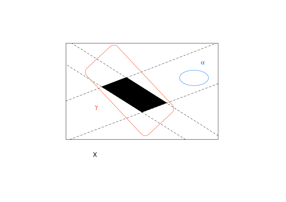
Figure 5: Pension Funds’ Market

6 Lagrangian Theory of a Closed Market

6.1 Hamilton Principle and Lagrange Equations

We will now enforce the minimal arbitrage principle $(A4)$ for the market portfolio strategy to derive the market dynamics for deflators and short rates. There exists an interaction between market portfolio and market dynamics: the market portfolio allocation is determined by the choices of all market participants and influence therefore the asset values. These -on their part- will influence the choices of the market participants and therefore the market portfolio. Everything happens simultaneously in time. Summarizing:

$$\boxed{\begin{array}[]{c}\text{Market dynamics for deflators and short rates }(D,r)=(D_{t},r_{t})\\ \upharpoonleft\downharpoonright\\ \text{Market Portfolio Strategy }x=x_{t}\end{array}}$$ (154)

If the market is closed, that is, if there is no external leverage, the market strategy must be self-financing. We denote by $x_{t}$ the dynamics of the market portfolio and by $(D_{t},r_{t})$ that of the deflators and short rates. By principle $(A4)$ these dynamics are characterized by the fact that they must be a. s. minimizer of the arbitrage action on the set of all self-financing strategies which are candidates for the market portfolio. Remark that we do not make any assumptions whether the market portfolio strategy allows for arbitrage or not, we just assume that it is a minimizer. The problem is intrinsically stochastic, but to tackle its solution by leveraging on the techniques developed by Cresson and Darses ([CrDa07]), we first analyze the deterministic case in order to later construct a solution for the stochastic case. To perform formal calculations we first introduce the Hamilton-Lagrange formalism of classical mechanics and follow Chapter $3$ of the beautiful [Ar89]. We first treat the deterministic case and embed the market portfolio strategy, deflators and short rate dynamics into one parameter family strategies, deflators and short rates. Then, we pass to stochastic processes following the results of [CrDa07], that we extend here to account for constraints to which the Lagrangian system is subject to.

Definition 59.

Let $\gamma$ be the market $\mathcal{D}$-admissible strategy, and $\delta\gamma$, $\delta D$, $\delta r$ be perturbations of the market strategy, deflators’ and short rates’ dynamics. The variation of $(\gamma,D,r)$ with respect to the given perturbations is the following one parameter family:

$$\epsilon\longmapsto(\gamma^{\epsilon},D^{\epsilon},r^{\epsilon}):=(\gamma,D,r)+\epsilon(\delta\gamma,\delta D,\delta r).$$ (155)

Thereby, the parameter $\epsilon$ belongs to some open neighborhood of $0\in\mathbf{R}$. The arbitrage action with respect to a positive martingale $\beta$ can be consistently defined by

$$\begin{split}A^{\beta}(\gamma;D,r)&:=\int_{\gamma}dt\left\{\mathcal{D}\rho^{\beta}+\operatorname{div}_{x}J\right\}=\\ &=\int_{\gamma}dt\left\{\mathcal{D}\log(\beta_{t}D_{t}^{x_{t}})+r_{t}^{x}\right\}=\\ &=\int_{0}^{T}dt\frac{x_{t}\cdot\mathcal{D}D_{t}+x_{t}\cdot(r_{t}D_{t})}{x_{t}\cdot D_{t}}+\log\frac{\beta_{T}}{\beta_{0}}.\end{split}$$ (156)

and the first variation of the arbitrage action as

$$\delta A^{\beta}(\gamma;D,r):=\frac{d}{d\epsilon}A^{\beta}(\gamma^{\epsilon};D^{\epsilon},r^{\epsilon})\mid_{\epsilon:=0}.$$ (157)

This leads to the following

Definition 60.

Let us introduce the notation $q:=(x,D,r)$ and $q^{\prime}:=(x^{\prime},D^{\prime},r^{\prime})$ for two vectors in $\mathbf{R}^{3N}$. The Lagrangian (or Lagrange function) is defined as

$$L(q,q^{\prime}):=L(x,D,r,x^{\prime},D^{\prime},r^{\prime}):=\frac{x\cdot(D^{\prime}+rD)}{x\cdot D}.$$ (158)

Lemma 61.

The arbitrage action for a self-financing strategy $\gamma$ is the integral of the Lagrange function along the $\mathcal{D}$-admissible strategy:

$$\begin{split}A^{\beta}(\gamma;D,r)&=\int_{\gamma}dt\,L(q_{t},q_{t}^{\prime})+\log\frac{\beta_{1}}{\beta_{0}}=\\ &=\int_{\gamma}dt\,L(x_{t},D_{t},r_{t},x_{t}^{\prime},D_{t}^{\prime},r_{t}^{\prime})+\log\frac{\beta_{1}}{\beta_{0}}.\end{split}$$ (159)

A fundamental result of classical mechanics allows to compute the extrema of the arbitrage action in the deterministic case as the solution of a system of ordinary differential equations.

Theorem 62 (Hamilton Principle).

Let us denote the derivative with respect to time as $\frac{d}{dt}=:\prime$ and assume that all quantities observed are deterministic. The local extrema of the arbitrage action satisfy the Lagrange equations under the self-financing constraints

$${\begin{split}&{\delta A^{\beta}(\gamma;D,r)=0\text{ for all }(\delta\gamma,\delta D,\delta r)}\\ &\text{such that }{x_{t}^{\prime}}^{\epsilon}\cdot D^{\epsilon}_{t}=0\text{ for all }\epsilon\end{split}}\Leftrightarrow\left\{\begin{array}[]{ll}\frac{d}{dt}\frac{\partial L}{\partial x^{\prime}}-\frac{\partial L}{\partial x}=+2\lambda D^{\prime}\\ \frac{d}{dt}\frac{\partial L}{\partial D^{\prime}}-\frac{\partial L}{\partial D}=-2\lambda x^{\prime}\\ \frac{d}{dt}\frac{\partial L}{\partial r^{\prime}}-\frac{\partial L}{\partial r}=0\\ x^{\prime}\cdot D=0,\end{array}\right.\\$$ (160)

where $\lambda\in\mathbf{R}$ denotes the constraint Lagrange multiplier.

Remark 63.

By Corollary 52, if the variation does not include deflators and short rates, the arbitrage action is constant on every homotopic equivalence class. Since we are looking for the optimal market strategy and asset market dynamics which minimizes the arbitrage, we have to vary over $\gamma$, $D$ and $r$ at the same time. This means that the integral of Lagrangian function takes values over a continuum and not over a discrete set as in the case of a fixed dynamics $D$ and $r$.

6.2 Stochastic Lagrangian Systems

In this subsection we briefly summarize and extend those contents of Cresson and Darses ([CrDa07]) needed in this paper. Cresson and Darses follow previous works of Yasue ([Ya81]) and Nelson ([Ne01]).

Definition 64.

Let $L=L(q,q^{\prime})$ be the Lagrange function of a deterministic Lagrangian system with the non holonomic constraint $C(q,q^{\prime})=0$. Setting $L_{\lambda}:=L-\lambda C$ for the constraint Lagrange multipliers the dynamics is given by the extended Euler-Lagrange equations

$$\boxed{\text{(EL)}\quad\left\{\begin{array}[]{l}\frac{d}{dt}\frac{\partial L_{\lambda}}{\partial q^{\prime}}(q,q^{\prime})-\frac{\partial L_{\lambda}}{\partial q}(q,q^{\prime})=0\\ C(q,q^{\prime})=0\end{array}\right.}$$ (161)

meaning by this that the deterministic solution $q=q_{t}$ and $\lambda\in\mathbf{R}$ satisfy the constraint and

$$\frac{d}{dt}\frac{\partial L_{\lambda}}{\partial q^{\prime}}\left(q_{t},\frac{dq_{t}}{dt}\right)-\frac{\partial L_{\lambda}}{\partial q}\left(q_{t},\frac{dq_{t}}{dt}\right)=0.$$ (162)

The formal stochastic embedding of the Euler-Lagrange equations is obtained by the formal substitution

$$S:\frac{d}{dt}\longmapsto\mathcal{D},$$ (163)

and allowing the coordinates of the tangent bundle to be stochastic

$$\boxed{\text{(SEL)}\quad\left\{\begin{array}[]{l}\mathcal{D}\frac{\partial L_{\lambda}}{\partial q^{\prime}}(q,q^{\prime})-\frac{\partial L_{\lambda}}{\partial q}(q,q^{\prime})=0\\ C(q,q^{\prime})=0\end{array}\right.}$$ (164)

meaning by this that the stochastic solution $Q=Q_{t}$ and the stochastic process $\lambda=\lambda_{t}$ satisfy the constraint and

$$\mathcal{D}\frac{\partial L_{\lambda}}{\partial q^{\prime}}\left(Q_{t},\mathcal{D}Q_{t}\right)-\frac{\partial L_{\lambda}}{\partial q}\left(Q_{t},\mathcal{D}Q_{t}\right)=0.$$ (165)

Definition 65.

Let $L=L(q,q^{\prime})$ be the Lagrange function of a deterministic Lagrangian system on a time interval $I$ with constraint $C=0$. Set

$$\Xi:=\left\{Q\in\mathcal{C}^{1}(I)\mid\mathbb{E}\left[\int_{I}|L_{\lambda}(Q_{t},\mathcal{D}Q_{t})|dt\right]<+\infty\right\}.$$ (166)

The action functional associated to $L_{\lambda}$ defined by

$$\boxed{\begin{aligned} &F:&\Xi\longrightarrow&\mathbf{R}\\ &&Q\longmapsto&\mathbb{E}\left[\int_{I}L_{\lambda}(Q_{t},\mathcal{D}Q_{t})dt\right]\end{aligned}}$$ (167)

is called stochastic analogue of the classic action under the constraint $C=0$.

For a sufficiently smooth extended Lagrangian $L_{\lambda}$ a necessary and sufficient condition for a stochastic process to be a critical point of the action functional $F$ is the fulfillment of the stochastic Euler-Lagrange equations (SEL): see Theorem 7.1 page 54 in [CrDa07]. Moreover we have the following

Lemma 66 (Coherence).

The following diagram commutes

$$\boxed{\lx@xy@svg{\hbox{\raise 0.0pt\hbox{\kern 81.38617pt\hbox{\ignorespaces\ignorespaces\ignorespaces\hbox{\vtop{\kern 0.0pt\offinterlineskip\halign{\entry@#!@&&\entry@@#!@\cr&\\&\crcr}}}\ignorespaces{\hbox{\kern-20.99237pt\raise 0.0pt\hbox{\hbox{\kern 0.0pt\raise 0.0pt\hbox{\hbox{\kern 3.0pt\raise 0.0pt\hbox{$\textstyle{L_{\lambda}(q_{t},q_{t}^{\prime})\ignorespaces\ignorespaces\ignorespaces\ignorespaces\ignorespaces\ignorespaces\ignorespaces\ignorespaces}$}}}}}}}\ignorespaces\ignorespaces\ignorespaces\ignorespaces{}{\hbox{\lx@xy@droprule}}\ignorespaces\ignorespaces\ignorespaces{\hbox{\kern 30.67885pt\raise 5.39166pt\hbox{{}\hbox{\kern 0.0pt\raise 0.0pt\hbox{\hbox{\kern 3.0pt\hbox{\hbox{\kern 0.0pt\raise-2.39166pt\hbox{$\scriptstyle{S}$}}}\kern 3.0pt}}}}}}\ignorespaces{\hbox{\kern 44.99237pt\raise 0.0pt\hbox{\hbox{\kern 0.0pt\raise 0.0pt\hbox{\lx@xy@tip{1}\lx@xy@tip{-1}}}}}}{\hbox{\lx@xy@droprule}}{\hbox{\lx@xy@droprule}}\ignorespaces\ignorespaces\ignorespaces\ignorespaces{}{\hbox{\lx@xy@droprule}}\ignorespaces\ignorespaces\ignorespaces{\hbox{\kern-81.38617pt\raise-20.0pt\hbox{{}\hbox{\kern 0.0pt\raise 0.0pt\hbox{\hbox{\kern 3.0pt\hbox{\hbox{\kern 0.0pt\raise-1.75pt\hbox{$\scriptstyle{\text{Critical Action Principle}}$}}}\kern 3.0pt}}}}}}\ignorespaces{\hbox{\kern 0.0pt\raise-29.5pt\hbox{\hbox{\kern 0.0pt\raise 0.0pt\hbox{\lx@xy@tip{1}\lx@xy@tip{-1}}}}}}{\hbox{\lx@xy@droprule}}{\hbox{\lx@xy@droprule}}{\hbox{\kern 44.99237pt\raise 0.0pt\hbox{\hbox{\kern 0.0pt\raise 0.0pt\hbox{\hbox{\kern 3.0pt\raise 0.0pt\hbox{$\textstyle{L_{\lambda}(Q_{t},\mathcal{D}Q_{t})\ignorespaces\ignorespaces\ignorespaces\ignorespaces}$}}}}}}}\ignorespaces\ignorespaces\ignorespaces\ignorespaces{}{\hbox{\lx@xy@droprule}}\ignorespaces\ignorespaces\ignorespaces{\hbox{\kern 72.05351pt\raise-20.0pt\hbox{{}\hbox{\kern 0.0pt\raise 0.0pt\hbox{\hbox{\kern 3.0pt\hbox{\hbox{\kern 0.0pt\raise-1.75pt\hbox{$\scriptstyle{\text{Stochastic Critical Action Principle}}$}}}\kern 3.0pt}}}}}}\ignorespaces{\hbox{\kern 72.05351pt\raise-29.5pt\hbox{\hbox{\kern 0.0pt\raise 0.0pt\hbox{\lx@xy@tip{1}\lx@xy@tip{-1}}}}}}{\hbox{\lx@xy@droprule}}{\hbox{\lx@xy@droprule}}{\hbox{\kern-14.27084pt\raise-40.0pt\hbox{\hbox{\kern 0.0pt\raise 0.0pt\hbox{\hbox{\kern 3.0pt\raise 0.0pt\hbox{$\textstyle{(EL)\ignorespaces\ignorespaces\ignorespaces\ignorespaces}$}}}}}}}\ignorespaces\ignorespaces\ignorespaces\ignorespaces{}{\hbox{\lx@xy@droprule}}\ignorespaces\ignorespaces\ignorespaces{\hbox{\kern 30.67885pt\raise-45.39166pt\hbox{{}\hbox{\kern 0.0pt\raise 0.0pt\hbox{\hbox{\kern 3.0pt\hbox{\hbox{\kern 0.0pt\raise-2.39166pt\hbox{$\scriptstyle{S}$}}}\kern 3.0pt}}}}}}\ignorespaces{\hbox{\kern 54.42851pt\raise-40.0pt\hbox{\hbox{\kern 0.0pt\raise 0.0pt\hbox{\lx@xy@tip{1}\lx@xy@tip{-1}}}}}}{\hbox{\lx@xy@droprule}}{\hbox{\lx@xy@droprule}}{\hbox{\kern 54.42851pt\raise-40.0pt\hbox{\hbox{\kern 0.0pt\raise 0.0pt\hbox{\hbox{\kern 3.0pt\raise 0.0pt\hbox{$\textstyle{(SEL)}$}}}}}}}\ignorespaces}}}}\ignorespaces} \textstyle{L_{\lambda}(q_{t},q_{t}^{\prime})\ignorespaces\ignorespaces\ignorespaces\ignorespaces\ignorespaces\ignorespaces\ignorespaces\ignorespaces} \scriptstyle{S} \textstyle{L_{\lambda}(Q_{t},\mathcal{D}Q_{t})\ignorespaces\ignorespaces\ignorespaces\ignorespaces} \textstyle{(EL)\ignorespaces\ignorespaces\ignorespaces\ignorespaces} \scriptstyle{S} \textstyle{(SEL)} \textstyle{L_{\lambda}(q_{t},q_{t}^{\prime})\ignorespaces\ignorespaces\ignorespaces\ignorespaces\ignorespaces\ignorespaces\ignorespaces\ignorespaces} \scriptstyle{S} \textstyle{L_{\lambda}(Q_{t},\mathcal{D}Q_{t})\ignorespaces\ignorespaces\ignorespaces\ignorespaces} \textstyle{(EL)\ignorespaces\ignorespaces\ignorespaces\ignorespaces} \scriptstyle{S} \textstyle{(SEL)}$$ (168)

6.3 Arbitrage Dynamics For Deflators, Short Rates And Market Portfolio

By means of the stochastization procedure (see subsection 6.2) we can extend Theorem 62 to the stochastic case:

Theorem 67 (Stochastic Hamilton Principle).

Let all quantities observed be stochastic and denote Nelson’s stochastic derivative with respect to time as $\mathcal{D}$. The local extrema of the expected arbitrage action satisfy the Lagrange equations under the self-financing constraints

$${\begin{split}&\delta\mathbb{E}_{0}[A^{\beta}(\gamma,D,r)]=0\text{ for all }(\delta\gamma,\delta D,\delta r)\\ &\text{such that }\mathcal{D}x_{t}^{\epsilon}\cdot D^{\epsilon}_{t}=-\frac{1}{2}\mathfrak{D}_{*}\left<x^{\epsilon},D^{\epsilon}\right>_{t}\text{ for all }\epsilon\end{split}}\Leftrightarrow\left\{\begin{array}[]{ll}\mathcal{D}\frac{\partial L}{\partial x^{\prime}}-\frac{\partial L}{\partial x}=+\mathcal{D}(\lambda D)\\ \mathcal{D}\frac{\partial L}{\partial D^{\prime}}-\frac{\partial L}{\partial D}=-\lambda\mathcal{D}x\\ \mathcal{D}\frac{\partial L}{\partial r^{\prime}}-\frac{\partial L}{\partial r}=0\\ (\mathcal{D}x)\cdot D=-\frac{1}{2}\mathfrak{D}_{*}{\left<x,D\right>},\end{array}\right.\\$$ (169)

almost surely.

Before we tackle the problem of solving the stochastic Euler-Lagrange equations, we remark that they satisfy the gauge invariance principle $(A3)$. As a matter of fact the Lagrange function definition is invariant with respect to a coordinate change in the tangent bundle $T\Upsilon$, where $\Upsilon:=j^{*}(\mathcal{B})$ is the pullback of the market bundle with respect to the embedding $j:X\rightarrow M,x\mapsto(x,0)$ (i.e. the market bundle without time component). In other words we can write

$$L:T\Upsilon\rightarrow\mathbf{R}.$$ (170)

We will first solve the deterministic Euler-Lagrange equations and then construct a stochastic solution by adding appropriate perturbations with zero mean. More exactly, we write the stochastic optimal solution as the sum of the deterministic one and a zero mean perturbation $\delta x,\delta D,\delta r\in\mathcal{C}^{1}$ (see Subsection 6.2) satisfying the conditions given by (172).

$$\begin{split}x_{t}&=\mathbb{E}_{0}[x_{t}]+\delta x_{t}\\ D_{t}&=\mathbb{E}_{0}[D_{t}]+\delta D_{t}\\ r_{t}&=\mathbb{E}_{0}[r_{t}]+\delta r_{t},\end{split}$$ (171)

whereas

$$\begin{matrix}&\mathbb{E}_{0}[\delta x_{t}]=0,&\mathcal{D}\delta x_{t}=0,&\delta x_{t}\cdot\delta D_{t}=0,&\mathbb{E}_{0}[x_{t}]\cdot\delta r_{t}\delta D_{t}=0\\ &\mathbb{E}_{0}[\delta D_{t}]=0,&\mathcal{D}\delta D_{t}=0,&\mathbb{E}_{0}[x_{t}]\cdot\delta D_{t}=0,&(\mathbb{E}_{0}[r_{t}]\mathbb{E}_{0}[D_{t}])\cdot\delta x_{t}=0\\ &\mathbb{E}_{0}[\delta r_{t}]=0,&\mathcal{D}\delta r_{t}=0,&\mathbb{E}_{0}[D_{t}]\cdot\delta x_{t}=0,&\delta x_{t}\cdot(\delta r_{t}\delta D_{t})=0\\ &\left<\delta x_{t},\delta D_{t}\right>=0.&&&\end{matrix}$$ (172)

We remark the Lagrange function satisfies $L(q,q^{\prime})=L(\mathbb{E}_{0}[q],\mathbb{E}_{0}[q^{\prime}])$ for any $q=(x,D,r)$ satisfying conditions (171) and(172). Now we will compute for the arbitrage case the deterministic solution of the Lagrange equations under the self-financing constraints, which explicitly written out read

$$\left\{\begin{split}&\left[\lambda_{t}(x_{t}\cdot D_{t})^{2}+(x_{t}\cdot D_{t})\right]D_{t}^{\prime}-\left[x_{t}\cdot D_{t}^{\prime}+x_{t}\cdot(r_{t}D_{t})-\lambda_{t}^{\prime}(x_{t}\cdot D_{t})^{2}\right]D_{t}+\\ &\quad+(x_{t}\cdot D_{t})(r_{t}D_{t})=0\\ &\left[\lambda_{t}(x_{t}\cdot D_{t})^{2}-(x_{t}\cdot D_{t})\right]x_{t}^{\prime}+\left[(x_{t}^{\prime}\cdot D_{t})-x_{t}\cdot(r_{t}D_{t})\right]x_{t}+\\ &\quad+(x_{t}\cdot D_{t})(x_{t}r_{t})=0\\ &x_{t}D_{t}=0\qquad\text{(this equation disappears if }r=0)\\ &x_{t}^{\prime}\cdot D_{t}=0.\end{split}\right.$$ (173)

This system of ODE can be solved and we obtain the following result in the case of the classic model model without futures.

Theorem 68 (Arbitrage Market Dynamics).

Let $r\equiv 0$. Then, the minimal arbitrage dynamics reads

$$\left\{\begin{split}x_{t}&=x_{0}+\delta x_{t}\\ D_{t}&=D_{0}+\delta D_{t}\\ \end{split}\right.$$ (174)

where $\delta x,\delta D$ and $\delta r$ are processes satisfying condition (172). In particular, the expectationat time $0$ of the portfolio market nominals and the asset deflators are constant over time and equal to their initial values.

Proof.

In the case $r\equiv 0$ the system of ODEs (173) becomes

$$\left\{\begin{split}&\left[\lambda_{t}(x_{t}\cdot D_{t})^{2}+(x_{t}\cdot D_{t})\right]D_{t}^{\prime}-\left[x_{t}\cdot D_{t}^{\prime}-\lambda_{t}^{\prime}(x_{t}\cdot D_{t})^{2}\right]D_{t}=0\\ &\left[\lambda_{t}(x_{t}\cdot D_{t})^{2}-(x_{t}\cdot D_{t})\right]x_{t}^{\prime}+\left[(x_{t}^{\prime}\cdot D_{t})\right]x_{t}=0\\ &x_{t}^{\prime}\cdot D_{t}=0.\end{split}\right.$$ (175)

It is a system of $2N+1$ first order ODEs in $2N+1$ unknown real values functions $(x,D,\lambda)$ of time. We see that

$$\left\{\begin{split}x_{t}&\equiv x_{0}\\ D_{t}&\equiv D_{0}\\ \lambda_{t}&\equiv\lambda_{0}\end{split}\right.$$ (176)

Since (175) is not a DAE system, by the Picard-Lindelöf theorem we conclude that this solution is unique. ∎

6.4 Symmetries, Conservation Laws and No-Arbitrage Dynamics

In this subsection we continue the study of the analogies between finance and classical mechanics with the Hamilton-Lagrange formalism and introduce the concept of symmetries of the asset model described by a Lagrangian on the principle fibre bundle. By Chapter $4$ of [Ar89] we will derive from symmetries conservation laws which hold true in the general case of an asset model allowing arbitrage or not. The short rates follow by the no-arbitrage principle by deriving the logarithm of the solution for deflators.

Definition 69 (Market Symmetry).

A bundle map $h:\Upsilon\rightarrow\Upsilon$ is called a symmetry of the market described by $(\Upsilon,L_{\lambda})$ if and only if there exists a real $\tilde{\lambda}$ such that

$$L_{\lambda}(T_{b}h.B)=L_{\tilde{\lambda}}(B)\quad\text{ for all }B\in T_{b}\Upsilon\,,\text{ for all }b\in\Upsilon.$$ (177)

Example 70 (Market Symmetries).

We represent term structures by their short rate, so that $b=(x,D,r)$ and $h=h(x,D,r)$.

• Rotation: $h(x,D,r):=[Sx;SD;S(rD)/(rD)]$, where $S$ is a orthogonal matrix, i.e. $S\in O(N)$. The division of two vectors is meant componentwise.

• Nominal Dilation: $h(x,D,r):=[sx;D;r]$, where $s$ is a non vanishing real number, i.e. $s\in\mathbf{R}^{*}$.

• Deflator Dilation: $h(x,D,r):=[x;sD;r]$, where $s$ is a non vanishing real number, i.e. $s\in\mathbf{R}^{*}$.

These examples all fulfill the definition of market symmetry, as one can see from the Lagrange function

$$L_{\lambda}(\underbrace{x,D,r}_{=q},\underbrace{x^{\prime},D^{\prime},r^{\prime}}_{=q^{\prime}})=\frac{x\cdot(D^{\prime}+rD)}{x\cdot D}-\lambda(x^{\prime}\cdot D).$$ (178)

The connection between symmetries and conservation laws in classical mechanics can be restated for our market model.

Theorem 71 (Noether).

Assume that all quantities observed are deterministic. Let $\{h_{\epsilon}\}_{\epsilon}$ be a one-parameter group of market symmetries $h_{\epsilon}:\Upsilon\rightarrow\Upsilon$ for the market described by $(\Upsilon,L_{\lambda})$. Then, the dynamics of market the portfolio, deflators and short rates have a first integral $I:T\Upsilon\rightarrow\mathbf{R}$. This means that there is a function, which writes

$$I(q,q^{\prime})=\frac{\partial L_{\lambda}}{\partial q^{\prime}}\frac{dh_{\epsilon}(q)}{d\epsilon}\mid_{\epsilon=0},$$ (179)

such that

$$\frac{d}{dt}I(q_{t},q^{\prime}_{t})=0$$ (180)

where $q=q_{t}$ is the solution of the deterministic Euler-Lagrange equations.

By means of the stochastization procedure as explained in Subsection 6.2, we can extend the preceding Theorem to the stochastic case (see [CrDa07] page 60):

Theorem 72 (Stochastic Version of Noether’s Result).

Let all quantities observed be stochastic and $\{h_{\epsilon}\}_{\epsilon}$ be a one-parameter group of market symmetries $h_{\epsilon}:\Upsilon\rightarrow\Upsilon$ for the market described by $(\Upsilon,L_{\lambda})$. Then, the dynamics of market the portfolio, deflators and short rates have a first integral $I:T\Upsilon\rightarrow\mathbf{R}$. This means that there is a function, which writes

$$I(q,q^{\prime})=\mathbb{E}_{0}\left[\frac{\partial L_{\lambda}}{\partial q^{\prime}}\frac{dh_{\epsilon}(q)}{d\epsilon}\mid_{\epsilon=0}\right],$$ (181)

such that

$$\frac{d}{dt}I(Q_{t},\mathcal{D}Q_{t})=0$$ (182)

where $Q=Q_{t}$ is the solution of the stochastic Euler-Lagrange equations.

In classical mechanics Noether’s Theorem is applied to a $N$ point particle system to derive the so called $10$ conservation laws for energy, momentum, angular momentum, and center of mass of an isolated system, i.e. with no external forces acting on its particles. Now we will derive conservation laws from the symmetries of a market with $N$ assets and no external leverage. That for, we have to extend the symmetries of our example to one parameter groups.

Example 73 (One Parameter Group of Market Symmetries).

• Rotations’ Group: $h_{\epsilon}(x,D,r):=[S_{\epsilon}x;S_{\epsilon}D;S_{\epsilon}(rD)/(rD))]$, where $S_{\epsilon}$ is a one parameter group of orthogonal matrices, i.e. $S_{\epsilon}\in O(N)$, and $S_{0}=I_{N}$, the identity matrix in $N$ dimensions. Therefore, $h_{0}(x,D,r)=[x;D;r]$. The first integral is

  $$I=\mathbb{E}_{0}\left[\frac{\partial L_{\lambda}}{\partial q^{\prime}}\Xi[x;D;e]\right],$$ (183)

  where $\Xi:=\operatorname{diag}(\xi,\xi,\xi)$ is a $3N\times 3N$ matrix, $\xi$ is a $N\times N$ antisymmetric matrix and $e=[1,\dots,1]^{\dagger}$. By Theorem (72) we obtain $(N-1)N/2$ non-trivial first integrals:

  $$\mathbb{E}_{0}\left[-\lambda_{t}D_{t}\cdot\xi x_{t}+\frac{x_{t}}{x_{t}\cdot D_{t}}\cdot\xi x_{t}\right]\equiv\text{ Time Constant.}$$ (184)

• Nominal Dilations’ Group: $h_{\epsilon}(x,D,r):=[(1+\epsilon)x;D;r]$, where $\epsilon$ is real number, so that $h_{0}(x,D,r)=[x;D;r]$. The first integral is

  $$I=\mathbb{E}_{0}\left[\frac{\partial L_{\lambda}}{\partial q^{\prime}}[x;0;0]\right],$$ (185)

  By Theorem (72) we obtain one non-trivial first integral:

  $$\mathbb{E}_{0}\left[-\lambda_{t}(x_{t}\cdot D_{t})\right]\equiv\text{ Time Constant.}$$ (186)

• Deflator Dilations’ Group: $h_{\epsilon}(x,D,r):=[x;(1+\epsilon)D;r]$, where $\epsilon$ is real number, so that $h_{0}(x,D,r)=[x;D;r]$. The first integral is

  $$I=\mathbb{E}_{0}\left[\frac{\partial L_{\lambda}}{\partial q^{\prime}}[0;D;0]\right].$$ (187)

  By Theorem (72) we obtain one trivial first integral, the $1$-constant function:

  $$\mathbb{E}_{0}\left[\frac{x_{t}\cdot D_{t}}{x_{t}\cdot D_{t}}\right]\equiv 1.$$ (188)

• Time Translations’ Group: since the time has been excluded by construction from the bundle $\Upsilon$, we cannot utilize Nöther’s result as depicted in Theorems 71 and 72. Therefore, we compute, for the deterministic case

  $$\begin{split}\frac{dL_{\lambda}}{dt}&=\frac{\partial L_{\lambda}}{\partial q}\cdot q^{\prime}+\frac{\partial L_{\lambda}}{\partial q^{\prime}}\cdot q^{\prime\prime}+\frac{\partial L_{\lambda}}{\partial t}=\\ &=\frac{\partial L_{\lambda}}{\partial q}\cdot q^{\prime}+\frac{d}{dt}\left[\frac{\partial L_{\lambda}}{\partial q^{\prime}}\cdot q^{\prime}\right]-\frac{d}{dt}\left[\frac{\partial L_{\lambda}}{\partial q^{\prime}}\right]\cdot q^{\prime}+\frac{\partial L_{\lambda}}{\partial t}.\end{split}$$ (189)

  Since the Euler-Lagrange equations are fulfilled, we obtain

  $$\frac{d}{dt}\left[\frac{\partial L_{\lambda}}{\partial q^{\prime}}\cdot q^{\prime}-L_{\lambda}\right]=-\frac{\partial L_{\lambda}}{\partial t}.$$ (190)

  Time translation invariance of $L_{\lambda}$ means $\frac{\partial L_{\lambda}}{\partial t}=0$, and, therefore

  $$\frac{\partial L_{\lambda}}{\partial q^{\prime}}\cdot q^{\prime}-L_{\lambda}\equiv\text{ Time Constant,}$$ (191)

  and in the stochastic case

  $$\mathbb{E}_{0}\left[\frac{\partial L_{\lambda}}{\partial q^{\prime}}\cdot q^{\prime}-L_{\lambda}\right]\equiv\text{ Time Constant,}$$ (192)

  which in our case reads

  $$\mathbb{E}_{0}\left[-\frac{x_{t}\cdot(r_{t}D_{t})}{(x_{t}\cdot D_{t})}\right]\equiv\text{ Time Constant.}$$ (193)

We can now utilize the results from the preceding example to complete Theorem 68 for the general case, where forwards are allowed as assets.

Theorem 74 (No Arbitrage Market Dynamics).

In a closed market satisfying the no-free-lunch-with-vanishing-risk condition, the dynamics for market portfolio strategy, deflators and term structures have constant expectations over time. More exactly the following identity holds a.s.

$$\begin{split}x_{t}&=x_{0}+\delta x_{t}\\ D_{t}&=D_{0}+\delta D_{t}\\ r_{t}&=r_{0}+\delta r_{t}\end{split}$$ (194)

where $\delta x,\delta D$ are processes satisfying condition (172).

Proof.

Let us consider the deterministic case and enrich the system of ODEs 173 with the equations obtained by Example 73. After some computations we obtain

$$\left\{\begin{split}&x_{t}\cdot(D_{t}^{\prime}+r_{t}D_{t})=0\\ &x_{t}\cdot(\lambda_{t}r_{t}D_{t}-\lambda_{t}^{\prime}D)=0\\ &x_{t}^{\prime}\cdot D_{t}=0\\ &\lambda_{t}(x_{t}\cdot D_{t})\equiv\text{const}\\ &\frac{x_{t}\cdot(r_{t}D_{t})}{(x_{t}\cdot D_{t})}\equiv\text{const}\\ &-\lambda_{t}D_{t}\xi x_{t}+\frac{x_{t}\cdot\xi x_{t}}{(x_{t}\cdot D_{t})}\equiv\text{const},\end{split}\right.$$ (195)

where $\xi$ is an arbitrary antisymmetric $N\times N$ matrix. By differentiating the equations where on the r.h.s. there is an unknown constant we get

$$\left\{\begin{split}&x_{t}\cdot(D_{t}^{\prime}+r_{t}D_{t})=0\\ &x_{t}\cdot(\lambda_{t}r_{t}D_{t}-\lambda_{t}^{\prime}D)=0\\ &x^{\prime}\cdot D_{t}=0\\ &\lambda_{t}^{\prime}(x_{t}\cdot D_{t})+\lambda_{t}(x_{t}^{\prime}\cdot D_{t})+\lambda_{t}(x_{t}\cdot D_{t}^{\prime})=0\\ &\left[x_{t}^{\prime}\cdot(r_{t}D_{t})+x_{t}\cdot(r_{t}^{\prime}D_{t})+x_{t}\cdot(r_{t}D_{t}^{\prime})\right](x_{t}\cdot D_{t})+\\ &\qquad-x_{t}\cdot(r_{t}D_{t})\left[(x_{t}^{\prime}\cdot D_{t})+(x_{t}\cdot D_{t}^{\prime})\right]=0\\ &(\lambda_{t}^{\prime}D_{t}\cdot\xi x_{t}-\lambda_{t}D_{t}^{\prime}\xi x_{t})(x_{t}\cdot D_{t})^{2}+(x_{t}^{\prime}\cdot\xi x_{t}+x_{t}\cdot\xi x^{\prime})(x_{t}\cdot D_{t})+\\ &\qquad-(x_{t}\cdot\xi x_{t})(x_{t}\cdot D_{t}^{\prime})=0,\end{split}\right.$$ (196)

By an appropriate choice of $\xi$ the system (196) becomes a system of $3N+1$ first order ODEs in $3N+1$ unknown real values functions $(x,D,r,\lambda)$ of time. We see that

$$\left\{\begin{split}x_{t}&\equiv x_{0}\\ D_{t}&\equiv D_{0}\\ r_{t}&\equiv r_{0}\\ \lambda_{t}&\equiv\lambda_{0}\end{split}\right.$$ (197)

Since (196) is not a DAE system, by the Picard-Lindelöf theorem we conclude that this solution is unique. Moreover, it fullfills the last equation of (196) for any $\xi$. The proof is completed.
∎

7 Conclusion

By introducing an appropriate stochastic differential geometric formalism the classical theory of stochastic finance can be embedded into a conceptual framework called Geometric Arbitrage Theory, where the market is modelled with a principal fibre bundle, arbitrage corresponds to its curvature and arbitrage strategies to its holonomy. The Fundamental Theorem of Asset Pricing is given a differential homotopic characterization. The market dynamics is seen to be the solution of stochastic Euler-Lagrange equations for a choice of the Lagrangian allowing to express Hamilton’s principle of minimal action as the minimal expected arbitrage principle, an extension of the no-arbitrage principle. Explicit are provided for a closed market.

References

- [Ar89] V. I. Arnold, Mathematical Methods of Classical Mechanics, Graduate Texts in Mathematics, Second Edition, Springer 1989.
- [BeFr02] F. Bellini and M. Frittelli, On the Existence of Minimax Martingale Measures, Mathematical Finance, 12/1, (1-21), 2002.
- [Bj04] T. Björk, Arbitrage Theory in Continuous Time, Oxford Finance, Second Edition, 2004.
- [BjHu05] T. Björk and H. Hult, A Note on Wick Products and the Fractional Black-Scholes Model, Finance & Stochastics, 9, No.2, (197-209), 2005.
- [Bl81] D. Bleecker, Gauge Theory and Variational Principles, Addison-Wesley Publishing, 1981, (republished by Dover 2005).
- [CrDa07] J. Cresson and S. Darses, Stochastic Embedding of Dynamical Systems, J. Math. Phys. 48, 2007.
- [DeSc08] F. Delbaen and W. Schachermayer, The Mathematics of Arbitrage, Springer 2008.
- [DuFoNo84] B. A. Dubrovin, A. T. Fomenko and S. P. Novikov, Modern Geometry-Methods and Applications: Part II. The Geometry and Topology of Manifolds, Springer GTM, 1984.
- [DuFiMu00] B. Dupoyet, H. R. Fiebig and D. P. Musgrov, Gauge Invariant Lattice Quantum Field Theory: Implications for Statistical Properties of High Frequency Financial Markets, Physica A 389 (107-116), 2010.
- [DeMe80] C. Dellachérie and P. A. Meyer, Probabilité et potentiel II - Théorie des martingales - Chapitres 5 à 8, Hermann, 1980.
- [El82] K. D. Elworthy, Stochastic Differential Equations on Manifolds, London Mathematical Society Lecture Notes Series, 1982.
- [Em89] M. Eméry, Stochastic Calculus on Manifolds-With an Appendix by P. A. Meyer, Springer, 1989.
- [Fa15] S. Farinelli, Geometric Arbitrage Theory and Market Dynamics, Journal of Geometric Mechanics, 7 (4), (431-471), 2015.
- [FaVa12] S. Farinelli and S. Vazquez, Gauge Invariance, Geometry and Arbitrage, The Journal of Investment Strategies, Volume 1/Number 2, Wiley, (23-66), Spring 2012.
- [FeJi07] M. Fei-Te and M. Jin-Long, Solitary Wave Solutions of Nonlinear Financial Markets: Data-Modeling-Concept-Practicing, Front. Phys. China, 2(3),(368-374), 2007.
- [FlHu96] B. Flesaker and L. Hughston, Positive Interest, Risk 9 (1), (115-124), 1996.
- [FöSc04] H. Föllmer and A. Schied, Stochastic Finance: An Introduction In Discrete Time, Second Edition, De Gruyter Studies in Mathematics, 2004.
- [Gl11] Y. E. Gliklikh, Global and Stochastic Analysis with Applications to Mathematical Physics, Theoretical and Mathemtical Physics, Springer, 2011.
- [HaTh94] W. Hackenbroch and A. Thalmaier, Stochastische Analysis. Eine Einführung in die Theorie der stetigen Semimartingale, Teubner Verlag, 1994.
- [Hö03] L. Hörmander, The Analysis of Linear Partial Differential Operators I: Distribution Theory and Fourier Analysis, Springer, 2003.
- [Hs02] E. P. Hsu, Stochastic Analysis on Manifolds, Graduate Studies in Mathematics, 38, AMS, 2002.
- [HuKe04] P. J. Hunt and J. E. Kennedy, Financial Derivatives in Theory and Practice, Wiley Series in Probability and Statistics, 2004.
- [Il00] K. Ilinski, Gauge Geometry of Financial Markets, J. Phys. A: Math. Gen. 33, (L5-L14), 2000.
- [Il01] K. Ilinski, Physics of Finance: Gauge Modelling in Non-Equilibrium Pricing, Wiley, 2001.
- [Ja98] J. D. Jackson, Classical Electrodynamics, Third Edition, Wiley, 1998.
- [KoNo96] S. Kobayashi and K. Nomizu, Foundations of Differential Geometry, Volume I, Wiley, 1996.
- [Ma96] P. N. Malaney, The Index Number Problem: A Differential Geometric Approach, PhD Thesis, Harvard University Economics Department, 1996.
- [Mo09] Y. Morisawa, Toward a Geometric Formulation of Triangular Arbitrage: An Introduction to Gauge Theory of Arbitrage, Progress of Theoretical Physics Supplement 179, (209-214), 2009.
- [Ne01] E. Nelson, Dynamical Theories of Brownian Motion, Second Edition, Princeton, 2001.
- [Pr10] Ph. E. Protter, Stochastic Integration and Differential Equations: Version 2.1, Stochastic Modelling and Applied Probability, Springer, 2010.
- [Ro94] L. C. G. Rogers, Equivalent Martingale Measures and No-Arbitrage, Stochastics, Stochastics Rep. 51, (41-49), 1994.
- [Scha01] W. Schachermayer, Optimal Investment in Incomplete Markets When Wealth May Become Negative, Annals of Applied Probability, 11, No. 3, (694-734), 2001.
- [Schw80] L. Schwartz, Semi-martingales sur des variétés et martingales conformes sur des variétés analytiques complexes, Springer Lecture Notes in Mathematics, 1980.
- [Sh00] S. E. Shreve, Stochastic Calculus for Finance, Vol. II, Springer, 2000.
- [Ši02] M. Šilhavý, The Mechanics and Thermodynamics of Continuous Media, Theoretical and Mathematical Physics, Springer, 2002.
- [SmSp98] A. Smith and C. Speed, Gauge Transforms in Stochastic Investment, Proceedings of the 1998 AFIR Colloquim, Cambridge, England, 1998.
- [St82] S. Sternberg, Lectures On Differential Geometry, Second Edition, Chelsea Pub. Co., 1982.
- [St00] D. W. Stroock, An Introduction to the Analysis of Paths on a Riemannian Manifold, Mathematical Surveys and Monographs, 74, AMS, 2000.
- [We06] E. Weinstein, Gauge Theory and Inflation: Enlarging the Wu-Yang Dictionary to a unifying Rosetta Stone for Geometry in Application, Talk given at Perimeter Institute, 2006.
- [Ya81] K. Yasue, Stochastic Calculus of Variations, Journal of Functional Analysis 41, (327-340), 1981.
- [Yo99] K. Young, Foreign Exchange Market as a Lattice Gauge Theory, Am. J. Phys. 67, (862-868), 1999.