Triplets of supermassive black holes:
Astrophysics, Gravitational Waves and Detection

Abstract

Supermassive black holes (SMBHs) found in the centers of many galaxies are understood to play a fundamental, active role in the cosmological structure formation process. In hierarchical formation scenarios, SMBHs are expected to form binaries following the merger of their host galaxies. If these binaries do not coalesce before the merger with a third galaxy, the formation of a black hole triple system is possible. Numerical simulations of the dynamics of triples within galaxy cores exhibit phases of very high eccentricity (as high as $e\sim 0.99$). During these phases, intense bursts of gravitational radiation can be emitted at orbital periapsis, which produces a gravitational wave signal at frequencies substantially higher than the orbital frequency. The likelihood of detection of these bursts with pulsar timing and the Laser Interferometer Space Antenna (LISA) is estimated using several population models of SMBHs with masses $\gtrsim 10^{7}~{}{\rm M_{\odot}}$. Assuming 10% or more of binaries are in triple systems, we find that up to a few dozen of these bursts will produce residuals $>1$ ns, within the sensitivity range of forthcoming pulsar timing arrays (PTAs). However, most of such bursts will be washed out in the underlying confusion noise produced by all the other ’standard’ SMBH binaries emitting in the same frequency window. A detailed data analysis study would be required to assess resolvability of such sources. Implementing a basic resolvability criterion, we find that the chance of catching a resolvable burst at a one nanosecond precision level is $2-50$%, depending on the adopted SMBH evolution model. On the other hand, the probability of detecting bursts produced by massive binaries (masses $\gtrsim 10^{7}{\rm M}_{\odot}$) with LISA is negligible.

1 Introduction

It is well established that most galaxies host supermassive black holes (SMBHs) in their centers (Richstone et al., 1998). In the past decade, compelling evidence of the correlation between the mass of the central SMBH and the bulge velocity dispersion and luminosity has been collected  (Ferrarese & Merritt, 2000; Gebhardt, et al., 2000; Merritt & Ferrarese, 2001; Tremaine et al., 2002), indicating a coevolutionary scenario for SMBHs and their hosts. On a cosmological scale, galaxy formation and evolution can be understood by semi-analytic modeling, where properties of the baryonic matter are followed in the evolving dark matter halos obtained from large-scale models of hierarchical gravitational structure formation. A simple model of galaxy and central SMBH evolution in which every merger of galaxies leads quickly to coalescence of their central black holes can quantitatively reproduce both the SMBH mass-bulge luminosity relation (Kauffmann & Haehnelt, 2000) and the SMBH mass-velocity dispersion relation (Haehnelt & Kauffmann, 2000).

In this general picture, if both of the galaxies involved in a merger host a SMBH, then the formation of a SMBH binary is an inevitable stage of the merging process. Following the merger, the two black holes sink to the center of the merger remnant because of dynamical friction  (Begelman, Blandford & Rees, 1980). When the mass (either in gas or stars) enclosed in their orbit is of the order of their own mass, they start to feel the gravitational pull of each other, forming a bound binary. The subsequent binary evolution is, however, still unclear. In order to coalesce, the binary must shed its binding energy and angular momentum; a dynamical process known in literature as ‘hardening’. A crucial point in assessing the fate of the binary is the efficiency with which it transfers energy and angular momentum to the surrounding gas and stars.

The case of SMBH binaries in stellar environments has received a lot of attention in the last decade. The system is usually modeled as a massive binary embedded in a stellar background with a given phase space distribution. The region of phase space containing stars that can interact with the SMBH binary in one orbital period is known as the loss cone (Frank & Rees, 1976; Amaro-Seoane & Spurzem, 2001; Milosavljević & Merritt, 2003). As the binary evolves, it ejects stars on intersecting orbits via the so called ‘slingshot mechanism’, causing a progressive emptying of the loss cone, which ultimately increases the hardening time scale. Without an efficient physical mechanism for repopulating the loss cone, the binary will never proceed to small separations where coalescence induced by gravitational radiation takes place within a Hubble time. This is known as the stalling or ‘last parsec’ problem (Milosavljević & Merritt, 2001).

In the last decade, several solutions to the stalling issue have been proposed. Axisymmetric or triaxial stellar distributions may significantly shorten the coalescence timescale (Yu, 2002; Merritt & Poon, 2004; Berczik, et al., 2006). This is bacause the presence of deviations from spherical symmetry can produce “boxy” orbits, as seen by Berczik, et al. (2006). These orbits produce centrophilic stellar orbits and, therefore, replenish the loss-cone. However, more recent calculations by Amaro-Seoane & Santamaria (2009) of the outcome of the merger of two clusters initially in parabolic orbits (Amaro-Seoane & Freitag, 2006) have not been able to reproduce the rotation necessary to create the unstable bar structure. Other studies have invoked eccentricities of the binary to refill the loss cone, since this effect could alter the cross section for super-elastic scatterings (thus altering the state of the loss cone) and shorten the gap to the onset of gravitational radiation effects (e.g.: Hemsendorf, Sigurdsson, & Spurzem 2002; Aarseth 2003a; Berczik, et al. 2006; Amaro-Seoane & Freitag 2006; Amaro-Seoane, Miller & Freitag 2009). The presence of massive perturbers may also help replenishing the loss cone, boosting the binary hardening rate (Perets et al., 2007). On the other hand, in smooth particle hydrodynamics simulations of SMBH binaries in gas-rich environments, efficient hardening induced by the tidal interaction between the binary and the gas medium has been observed, indicating a possible quick coalescence (Escala et al., 2005; Dotti et al., 2006a). However, current simulations do not have the resolution to follow the binary fate down to the gravitational wave (GW) emission regime, and robust conclusions about its late inspiral and coalescence can not be drawn. In any case, very massive low redshift systems, which are the major focus of our study, are more likely to reside in massive gas poor galaxies and their dynamics is probably dominated by stellar interactions.

When scaled to very massive binaries (masses $>10^{8}{\rm M}_{\odot}$), the inferred coalescence timescales in a stellar dominated environment are of the order of few Gyrs, indicating that SMBH binaries may be relatively long living systems. If the typical timescale between two subsequent mergers is comparable the SMBH binary lifetime, then a third black hole may reach the nucleus when the binary is still in place, and the formation of SMBH triplets might be a common step in the galaxy formation process. Recent studies of galaxy pairs lead to the conclusion that $30-70$% of present day massive galaxies have undergone a major merger since redshift one (Bell et al., 2006; Lin et al., 2008), where ’major’ means with baryonic mass ratio of the two components larger than $1/3$ or $1/4$ (depending on the study), which is a quite conservative threshold. This means that, on average, all massive galaxies have experienced a merger event in the last ten billion years. Assuming uncorrelated events, and a typical binary lifetime of one billion years, then 10% of SMBH binaries may form a triplet. With increasing redshift (and decreasing masses), dynamical timescales become shorter and shorter, implying that triplets may have been more common in the high redshift Universe.

In this paper we focus on SMBH triplets, studying their dynamical evolution, GW emission, and detectability. Employing sophisticated three body scattering experiments calibrated on direct-summation Nbody simulations, we study the dynamical evolution of the system, finding surprisingly high eccentricities of the inner SMBH binary (up to $e>0.99$). Even though the triple interaction would possibly lead to an ejection of one or even all SMBHs (Valtonen, et al., 1994), most of the systems are long living ($\sim 10^{9}$ yrs, Hoffman & Loeb (2007)), and final coalescence is more common than ejection, confirming analytical results by Makino & Ebisuzaki (1996). We model at the leading quadrupole order (Peters & Mathews, 1963) the bursts of gravitational radiation emitted in the highly eccentric phase, assessing detectability with future GW experiments. Adopting cosmologically and astrophysically motivated models for SMBH formation and evolution, we estimate reliable event rates.

In order to cover the low frequencies generated by the expected cosmological population of coalescing SMBH binaries (e.g., Wyithe & Loeb, 2003; Sesana et al., 2004, 2005; Sesana, Volonteri & Haardt, 2007) or plunges of compact objects such as stellar black holes on to supermassive ones (see e.g. Amaro-Seoane et al., 2007, for a review and references therein), the space-born observatory LISA (Bender et al., 1998) has been planned to be covering the range of frequencies of $\sim 10^{-4}-10^{-1}~{}{\rm Hz}$. Moving to even lower frequencies, the Parkes Pulsar Timing Array (PPTA,  Manchester, 2006, 2008), the European Pulsar Timing Array (EPTA,  Janssen et al., 2008) and the North American Nanohertz Observatory for Gravitational Waves (NANOGrav,  Jenet et al., 2009) are already collecting data and improving their sensitivity in the frequency range of $\sim 10^{-8}-10^{-6}$ Hz, and in the next decade the planned Square Kilometer Array (SKA,  Lazio, 2009) will provide a major leap in sensitivity.

Throughout this paper we consider only very massive systems, with total mass $\sim 10^{8}{\rm M}_{\odot}$. Our goal is to investigate if the high frequency nature of eccentric bursts can provide information about systems which would otherwise emit outside the frequency windows of the planned GW experiments quoted above, by shifting wide (separation $\gtrsim 0.1$ pc) SMBH binaries into the PTA window or by boosting relatively massive (masses $>10^{7}{\rm M}_{\odot}$) systems into the LISA domain. We note that the bursts analyzed here are different from the ‘bursts with memory’, which arise during the actual coalescence of SMBH binaries and are discussed in Pshirkov, Baskaran & Postnov (2009) and van Haasteren & Levin (2009).

The structure of the paper is as follows. In Section 2, we describe our comprehensive study of the dynamics of triple systems and investigate the eccentricity evolution of the inner binary by using direct-summation $N-$body techniques and a statistical 3-body sample calibrated on the $N-$body results. In Section 3, we model the GW signal produced by eccentric bursts and we introduce observable quantities for PTAs and LISA. In Section 4 we construct detailed populations of emitting SMBH binaries and triplets, and we discuss our results in terms of signal observability and detection rates in Section 5. Lastly, we briefly summarize our results in Section 6.

2 Dynamics of triple systems

In modeling the dynamics of black hole triple systems within the centres of galaxy merger remnants, direct $N$-body integrations provide the most accuracy but are the most computationally expensive. We performed eight direct $N$-body calculations and used these to test the validity of an approximation scheme involving three-body SMBH dynamics embedded in a smoothed galactic potential with dynamical friction and gravitational radiation modeled by drag forces.

2.1 Direct $N-$body calculations

The direct-summation Nbody method we employed for all the calculations includes the KS regularisation. Thus, when two particles are tightly bound to each other or the separation between them becomes very small during a hyperbolic encounter, the system becomes a candidate to be regularised in order to avoid problematical small individual time steps (Kustaanheimo & Stiefel, 1965). This procedure was later exported to systems involving more than two particles. In particular, the KS regularisation has been adapted to isolated and perturbed 3– and 4–body systems—the so-called triple (unperturbed 3-body subsystems), quad (unperturbed 4-body subsystems) and the chain regularisation. The latter is invoked in our simulations whenever a regularised pair has a close encounter with another single star or another pair (Aarseth, 2003b).

The basis of direct Nbody codes relies on an improved Hermite integrator scheme (Aarseth, 1999) for which we need not only the accelerations but also their time derivative. The computational effort translates into accuracy so that we can reliably keep track of the orbital evolution of every particle in our system. In order to make a highly accurate estimate of the eccentricity evolution of the SMBH system, we do not employ a softening to the gravitational force (i.e. substituting the $1/r^{2}$ factor with $1/(r^{2}+\epsilon^{2})$, where $r$ is the separation and $\epsilon$ the softening parameter) that weakens the interaction at small separations.

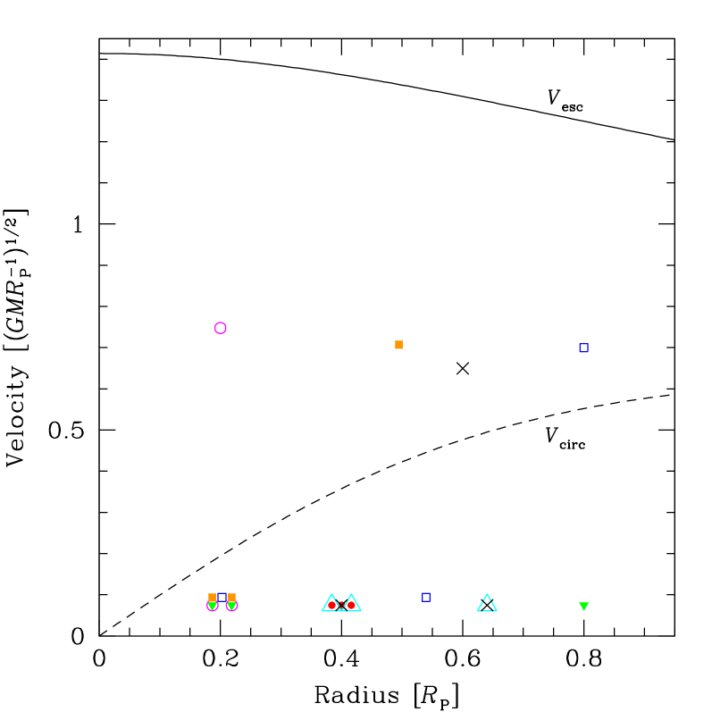
Figure 1: Initial conditions for the different direct $N$-body simulations in the $R_{\rm P}$, $V$ plane. For each simulation we choose the separation between two SMBHs to be substantially smaller than the distance to the third SMBH. The initial parameters are selected in such a way that they are random but with an initial velocity smaller than the escape velocity $V_{\rm esc}$ and with a radius $r<R_{\rm P}$. We also show the circular velocity in the figure, $V_{\rm circ}$. Initially The set of 3 SMBHs of simulation A is represented with red solid bullets; for simulation B with green solid triangles; for simulation C with cyan open triangles; for simulation D with blue open squares; for simulation E with pink open circles; for simulation H with solid orange squares and for simulations F and G with black crosses. In the case of simulations A, B, C, D, E, F and G the three SMBHs are set initially in a planar configuration. In the case of simulation H they have a z component different from zero in both the coordinates and velocities. In the cases of simulations A, B, C, E and H we slightly modified the positions of the symbols in order to avoid an overlap

Model	A	B	C	D	E	F	G	H
${\cal N}_{\star}$	64,000	64,000	64,000	64,000	64,000	64,000	512,000	256,000
$R/{R}_{\rm P}$	0.40012	0.80006	0.40012	0.80006	0.20025	0.60017	0.60017	0.49497
	0.40012	0.20303	0.64031	0.53956	0.20303	0.64031	0.64031	0.20278
	0.40012	0.20303	0.40012	0.20303	0.20303	0.40012	0.40012	0.20278
$V/{V}_{\rm esc}$	0.07476	0.07476	0.07476	0.70000	0.74762	0.64991	0.64991	0.70711
	0.07476	0.07476	0.07476	0.09345	0.07476	0.07476	0.07476	0.09345
	0.07476	0.07476	0.07476	0.09345	0.07476	0.07476	0.07476	0.09345
$V/{V}_{\rm circ}$	0.20886	0.13543	0.20886	1.26802	3.84516	1.36391	1.36391	1.68376
	0.20886	0.37956	0.15108	0.20886	0.37956	0.15108	0.15108	0.47496
	0.20886	0.37956	0.20886	0.47442	0.37956	0.20886	0.20886	0.47496

Table 1: Initial conditions for the set of three SMBHs in each of the eight direct $N$-body simulations. ${\cal N}_{\star}$ is the total number of stars employed in the simulation, ${V}$ their velocity, $R$ their position, ${R}_{\rm P}$ the position of the SMBHs in terms of the Plummer radius, ${V}_{\rm esc}$ their escape velocity and ${V}_{\rm circ}$ is their circular velocity. The mass of the SMBHs in $N-$body units is $1\cdot 10^{-2}$, they are equal-mass and the mass of a star $1.15\cdot 10^{-5}$

The initial conditions for the set of three SMBHs, used to conduct an exploration of the initial parameter space are shown in Table 1. For the stellar system, we use a Plummer model (Plummer, 1911), which is an $n=5$ polytrope with a compact core and an extended outer envelope. In this model the density is approximately constant in the centre and drops to zero in the outskirts, $\phi=-{GM_{\star}}/{\sqrt{r^{2}+R_{\rm P}^{2}}}$, with $M_{\star}$ the total stellar mass. This defines the Plummer radius $R_{\rm P}$. We depict the initial conditions in Figure 1, relative to the circular and escape velocity of the Plummer potential. We present results from eight direct numerical simulations, one using 512,000 stars using the special-purpose GRAPE6 system and the remaining simulations using Beowulf PC clusters and the AEI mini-PCI GRAPE cluster Tuffstein.

2.2 Three-body improved statistics

While direct $N$-body simulations yield a very accurate result, they should be seen as a way to calibrate and test faster, more approximate simulations which can exhaustively cover the parameter space and provide good statistics. We note that the SMBHs in the $N-$body simulations are equal-mass and (with the exception of simulation H), all of the systems studied with this method are coplanar. This was done because setting all SMBHs on a single plane accelerates the dynamics, shortening the integration time.

In general, one wants to explore the whole parameter space, including non coplanar systems with different SMBH masses. For this purpose, we performed an ensemble of 1000 three-body experiments, with the three Euler angles of the outer orbit sampled uniformly and a distribution of mass ratios motivated by Extended Press-Schechter theory (with typical mass ratios ${\rm m_{1}:m_{2}:m_{3}}$ around 3.5:1). In each experiment we computed the Newtonian orbits of three SMBHs embedded in a smooth galactic potential and added drag forces to account for gravitational radiation and dynamical friction. We also included coalescence conditions when either of the two SMBHs pass within three Schwarzschild radii of each other, or the gravitational radiation timescale becomes short relative to the orbital period of the binary. Close triple encounters were treated using a KS-regularised few-body code provided by Sverre Aarseth (Mikkola & Aarseth, 1990, 1993), while the two-body motion in between close encounters was followed with a simple 4th-order Runge-Kutta integrator. See Hoffman & Loeb (2007) for further details on the code. The initial conditions are those for the canonical ICs as in Hoffman & Loeb (2007). We performed each run twice—once with gravitational radiation drag and the coalescence conditions, and once without.

The 3-body experiments are divided into two computational regimes based upon a dimensionless parameter, $\alpha$, that measures the relative tidal perturbation to the inner binary by the interloper at apoapsis:

$$\alpha=2\frac{R_{\rm apo}^{3}\,M_{\rm single}}{M_{\rm bin,\,smaller}\,D_{\rm single}^{3}},$$ (1)

where $R_{\rm apo}$ is the apoapsis separation of the two inner binary members, $M_{\rm single}$ is mass of the single SMBH, $M_{\rm bin,\,smaller}$ is mass of the smaller inner binary member and $D_{\rm single}$ is the distance of the interloper (single SMBH) from the inner binary centre-of-mass. In the limit $\alpha\rightarrow$ 0, we know that the period of the inner binary is perfectly Keplerian (plus gravitational radiation), since the perturbation to the force from the third body is negligible, and thus we can do orbit-averaged integration instead of precisely integrating the trajectories of all three bodies. The two regimes are defined as follows:

1. The first regime corresponds to when a 3-body interaction is taking place (defined by $\alpha>10^{-5}$), an extremely conservative criterion for when we need to do the full three-body integration.

2. The second regime corresponds to when the single SMBH and binary are wandering separately through the galaxy ($\alpha<10^{-5}$), often on the order of a Hubble time.

In regime (i) the 3-SMBH dynamics is integrated using Sverre Aarseth’s high-precision, regularised CHAIN code. Gravitational radiation and stellar-dynamical friction are treated as perturbing, velocity-dependent forces on the three separate bodies. In regime (ii) the separate orbits of the single and binary centre-of-mass are followed using a simple 4th-order Runge-Kutta integrator and the evolution of the binary semi-major axis and eccentricity are evolved using orbit-averaged equations.

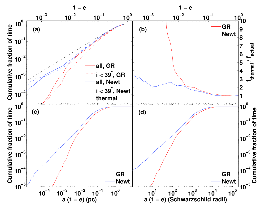
Figure 2: Cumulative fraction of time for the set of 1000 three-body simulations. The red, solid line corresponds to all simulations with the 2.5 post-Newtonian correction term; the blue, solid line corresponds to the same simulations but without it (i.e. purely Newtonian); the dot-dashed red curve is like the first case but taking into account only systems in which the third SMBH had an inclination below the critical Kozai angle of $39^{\circ}$, to compare with the direct $N$-body simulations of Fig.(4); the dot-dashed blue curve is the same, but for the Newtonian cases and the dot-dashed black curve corresponds to the thermal distribution, since the direct $N$-body simulations do not have relativistic correction terms. The top left panel shows the eccentricity computed from the instantaneous positions and velocities of the two binary members, and the top right panel shows the ratio of the actual to the thermal distribution. For the Newtonian runs, the distribution is within a factor of 2 of thermal down to $1-e=0.01$ and within a factor of 3 of thermal down to $\sim 1-e=0.001$. The bottom two panels show the pericenter distances of the binary in pc and in units of the sum of the Schwarzschild radii of the two binary members. No coalescence was allowed during close encounters for the Newtonian runs. We can see that the distributions converge, with respect to the statistics, from the fact that they are substantially the same as the lower-number experiments and that the Newtonian and gravitational radiation distributions match at low eccentricities

Figure 3: Time spent at different locations in the $t_{\rm gr}$ - (1-e) plane in the Newtonian simulations (blue lines) of Figure 2. $P=t/t_{\rm close}$ is the probability of finding the binary in a given bin at a randomly chosen time, where $t_{\rm close}$ is the total simulation time spent in close 3-body encounters. The simulation being presented here is the same as the Newtonian simulation (blue lines) in Figure 2. The purpose of this figure is to understand whether gravitational radiation is the main reason for the fall-off in the eccentricity distribution, since the highest eccentricity systems have short coalescence times and quickly disappear. $t_{\rm gr}$ is in years in the upper panel and in orbital periods in the lower panel (the typical resonant encounter takes on order $10^{5}$ yrs). Note that 1-e = 0.002 is about where $t_{\rm gr}$ falls to less than an orbital period

In computational regime (ii) (between 3-body encounters), the stellar interactions are treated using the hard binary prescription of Quinlan (1996). The eccentricity evolution of the inner binary under stellar interactions for near equal-mass hard binaries is quite weak so it is neglected entirely and only the binary semi-major axis is evolved under stellar interactions. The eccentricity is evolved under gravitational radiation as given by Peters (1964). Dynamical friction tends to increase the eccentricity of a binary in the supersonic regime (where the orbital speed exceeds the stellar velocity dispersion), and to circularize it in the subsonic regime. Since the triple SMBH system starts out supersonic in these 3-body experiments, this effect produces a slight increase in the outer binary eccentricity during the initial inspiral of the third SMBH. Although we neglect the eccentricity evolution of the inner binary during this phase, we find that its eccentricity is thermalized by the first resonant 3-body encounter. The timescale of the chaotic 3-body interactions ($\sim 10^{5}$ yr) is much shorter than the stellar-dynamical timescale ($~{}10^{7}-10^{10}$ yr), so any effect of stellar interactions during these encounters is completely negligible. Thus, stellar interactions play only two roles in our 3-body simulations:

1. They bring the third BH in to interact with the inner binary from an initial marginally stable hierarchical triple configuration;

2. During phase (ii), stellar-dynamical interactions gradually decrease the binary semi-major axis, so that it enters the next three-body encounter harder than it left the last one if the time between encounters is long ( $>~{}10^{7}$ yrs). The binary may even coalesce between encounters due to this gradual shrinking.

Consequently, the distribution in eccentricities is best estimated using the fraction of time that binaries spend at a given eccentricity while in computational regime (i) since there is minimal evolution of the eccentricity while in regime (ii). We note that the overwhelming majority of the time spent in regime (i) is still spent with $\alpha$ small enough that the system can be though of as a separate inner and outer binary, and so the instantaneous inner binary semi-major axis and eccentricity are well-defined.

2.3 Distribution of Eccentricities

Figure 2a shows the fraction of the time that the binary (closest SMBH pair) spends above a given eccentricity during close encounters, averaged over 1000 three-body experiments. The red solid curves are the results of the standard runs including gravitational radiation drag and coalescence conditions while the blue solid curves are the “Newtonian” case with these effects neglected. The dashed red and blue curves are averaged over only those experiments where the initial BH configuration has inclination $<39^{\circ}$, the critical angle for Kozai oscillations, for comparison with the direct $N$-body simulations that use coplanar initial conditions. The black (dot-dashed) line shows the thermal distribution of eccentricities for reference purposes. Three-body interactions result in a thermal distribution of eccentricities, truncated at very high eccentricities by coalescence in collisions when gravitational radiation is included. The similarity of the dashed and solid curves shows that once the initial secular evolution is over, the system quickly thermalizes and little memory of the initial configuration is maintained. Figure 2b shows the ratio of the thermal to the actual distribution as a function of eccentricity. The first close encounter in each experiment has been excluded from these plots, since it begins from a stable hierarchical triple configuration and includes a long period of secular evolution, whereas chaotic three-body encounters are the focus of this work.

The runs with and without gravitational radiation closely follow each other and the thermal distribution up to eccentricities $e\sim 0.99$. At higher eccentricities, the Newtonian distribution remains within a factor of 2 to 3 of the thermal distribution, but the gravitational radiation curve falls off sharply, since these high-eccentricity systems coalesce quickly through emission of gravitational waves. To verify this interpretation of Figure 2, we plot the time spent at different locations in the $t_{gr}$-$(1-e)$ plane in Figure 3, where the gravitational radiation timescale is computed from the instantaneous $(a,e)$ of the binary. The eccentricity where the red and blue curves diverge in Figure 2b ($1-e\sim 0.01$) is the value where the typical $t_{gr}$ falls to just a few orbital periods, so that the binary can coalesce quickly by gravitational radiation before the third body scatters it on to a lower-eccentricity orbit. Figures 2c-d show the time spent by the binary at various pericenter separations, in pc and in Schwarzschild radii. Note that the gravitational radiation curve diverges sharply from the Newtonian one when the pericenter separation reaches $\sim$100 Schwarzschild radii. We show the fraction of time spent at different eccentricities and the fraction of time spent at different pericenter separations for the $N-$body simulations in Figure 4. The qualitative features are retained.

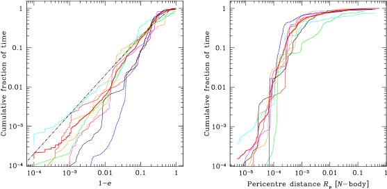
Figure 4: Left panel: Fraction of time for the direct $N$-body simulations at which the binary black hole has eccentricity in the range $1-e$ for the 512,000 stars simulation (thin green curve) and for the lower-resolution simulations. The thick red curve corresponds to the average of these lower-resolution computations and the dashed curve to the thermal distribution. Right panel: Cumulative fraction of time spent on a certain periapsis distance for all direct $N$-body simulations following the same colour labelling. One $N-$body unit of distance is ${\cal U}|_{\rm R}=1.1$ pc

3 Gravitational waves: analysis of the signal

In this section we make use of the leading Newtonian order derivation of the GW radiation from eccentric binaries, as described in Peters & Mathews (1963). We also use of geometric units, with $G=c=1$. Consider a system with masses $M_{2}<M_{1}$ orbiting with an orbital rest frame frequency $f_{r}=\omega/2\pi$, and with eccentricity $e$; at the quadrupole leading order, the luminosity $\dot{E}$ emitted by the system averaged over one complete orbit is:

$$\dot{E}=\frac{32}{5}{\cal M}^{10/3}(2\pi f_{r})^{10/3}F(e)=\dot{E}_{c}F(e)$$ (2)

where

$$F(e)=\sum_{n=0}^{\infty}g(n,e)=\frac{1+\frac{73}{24}e^{2}+\frac{37}{96}e^{4}}{(1-e^{2})^{7/2}},$$ (3)

and ${\cal M}=M_{1}^{3/5}M_{2}^{3/5}/(M_{1}+M_{2})^{1/5}$ is the chirp mass of the system. $\dot{E}_{c}$, defined by the right-hand side in equation (2), is the luminosity emitted by a circular binary orbiting at the same frequency $f_{r}$. The binary radiates GWs in the whole spectrum of harmonics $f_{r,n}=nf_{r}\,\,\,(n=1,2,...)$, and the relative power radiated in each single harmonic is described by the function $g(n,e)$, defined as:

$$g(n,e)=\frac{n^{4}}{32}\left(B_{n}^{2}+\left(1-e^{2}\right)A_{n}^{2}+\frac{4}{3n^{2}}J_{n}(ne)^{2}\right),$$ (4)

where $J_{n}(x)$ are the Bessel functions and $A_{n}$ and $B_{n}$ are also defined in terms of the $J_{n}$ as:

$$B_{n} = J_{n-2}(ne)-2eJ_{n-1}(ne)+\frac{2}{n}J_{n}(ne)$$ (5)

$$+2eJ_{n+1}(ne)-J_{n+2}(ne)$$

$$A_{n} = J_{n-2}(ne)-2J_{n}(ne)+J_{n+2}(ne).$$ (6)

The total luminosity of the source can then be written, using equations (2) and (3), as the sum of the component radiated at each single harmonic:

$$\dot{E}=\sum_{n=0}^{\infty}\dot{E}_{n}=\sum_{n=0}^{\infty}\dot{E}_{c}g(n,e).$$ (7)

Given a general GW characterised by the two polarised component waves $h_{+}$ and $h_{\times}$, the rms amplitude of the wave is defined as $h=\sqrt{\langle h_{+}^{2}+h_{\times}^{2}\rangle}$, where $\langle\ \ \rangle$ denotes the average over directions and over time. The flux radiated in the GW field is related to the derivatives of its amplitude components by the relation (Thorne, 1987)

$$\frac{dE}{dtdA}=\frac{1}{16\pi}\left(\dot{h}_{+}^{2}+\dot{h}_{\times}^{2}\right).$$ (8)

The sinusoidal nature of the waves implies $\langle\dot{h}_{+}^{2}+\dot{h}_{\times}^{2}\rangle=4\pi^{2}f_{r}^{2}\langle h_{+}^{2}+h_{\times}^{2}\rangle$. So that integrating equation (8) over a spherical surface of radius $d_{L}$ (the luminosity distance from the source) centered at the source and averaging over an orbital period, directly relates $\dot{E}$ to the wave rms amplitude. We can then infer that the rms amplitude and the energy radiated in the n-th harmonic are related as (Finn & Thorne, 2000)

$$h_{n}=\frac{1}{\pi d}\frac{\sqrt{\dot{E}_{n}}}{f_{r,n}}=2\sqrt{\frac{32}{5}}\frac{{\cal M}^{5/3}}{nd_{L}}(2\pi f_{r})^{2/3}\sqrt{g(n,e)},$$ (9)

where $d=d_{L}/(1+z)$. In the limit of a circular orbit (i.e., $g(n,e)=\delta_{n,2}$ in the Kronecker-$\delta$ notation), equation (9) returns the usual sky-polarization averaged amplitude (Thorne, 1987).

3.1 Observed quantities

Since we are interested in an estimate of the detectability of extremely eccentric binaries (induced by triple interactions) by means of pulsar timing (and possibly LISA) observations, we first introduce an extension of the characteristic amplitude to include eccentric binaries. Eccentric binaries emit pulses of GWs at their periapsis passages, and the rms amplitude of each harmonic is given by equation (9). However, $h_{n}$ is an average amplitude related to the average luminosity along the orbit. The actual relevant time for the burst is the periapsis passage timescale $T_{p}=(1-e)^{3/2}T_{\rm orb}$ ($T_{\rm orb}$ is the binary orbital period), and if the burst is detected, almost all the energy radiated along the whole orbit is seen on the timescale $T_{p}$. This means that the relevant detectable amplitude of each harmonic during the burst is

$$h_{\rm obs,n}=h_{n}\sqrt{{\cal T}f_{r,n}},$$ (10)

where the factor ${\cal T}={\rm max}(T_{\rm orb},T_{\rm obs})$ takes into account the fact that, if $T_{\rm orb}<T_{\rm obs}$, multiple bursts are visible during the observation. Equation (10) is a crude approximation, nevertheless it catches the basic features of the observed signal: this is given by the rms amplitude of each single n-th harmonic multiplied by the square root of the cycles completed by the harmonic in an orbital period, assuming that the binary orbit is a fixed ellipse and GW emission does not change the orbital parameters.

The search for GWs using pulsar timing data exploits the effect of gravitational radiation on the propagation of the radio waves from one (or more) pulsar(s). A passing GW would imprint a characteristic signature on the time of arrival of radio pulses (e.g. Sazhin 1978; Detweiler 1979; Bertotti, Carr & Rees 1983), producing a so called timing residual. We refer the reader to Jenet et al. (2004) and Sesana, Vecchio & Volonteri (2009), (hereinafter SVV09) for a detailed mathematical description of the GW induced residuals. The residuals are defined as integrals of the GW during the observation time. For a collection of harmonics, the residuals are given by:

$$R(T)=\int_{0}^{T}{\sum_{n=0}^{\infty}\left(\frac{\alpha^{2}-\beta^{2}}{2(1+\gamma)}h_{+,n}+\frac{\alpha\beta}{(1+\gamma)}h_{\times,n}\right)dt},$$ (11)

where $\alpha$, $\beta$, and $\gamma$ are the direction cosines of the pulsar relative to a Cartesian coordinate system defined with the $z$-axis along the direction of propagation of the gravitational wave and the $x$ and $y$ axes defining the $+$ polarization. The harmonics of the two polarizations, $h_{+,n}$ and $h_{\times,n}$, can be found in Section 3.2 of Pierro, et al. (2001). The rms residual $\delta t_{\mathrm{gw}}$ is then formally defined as $\sqrt{\langle R(T)^{2}\rangle}$.

A simple derivation of the average timing residual $\delta t_{\mathrm{gw}}$ generated by a circular binary is given by SVV09. With the notations adopted above, their equation (20) reads:

$$\delta t_{\mathrm{gw}}(f)=\sqrt{\frac{8}{15}}\frac{h_{2}}{2\pi f_{r}}\sqrt{fT_{\rm obs}}\,,$$ (12)

where the observed frequency $f$ is related to $f_{r}$ as $f=f_{r}/(1+z)$ (being $z$ the redshift of the source), the factor $\sqrt{fT_{\rm obs}}$ takes into account for the signal ’build-up’ with the square root of the number of cycles, and $\sqrt{8/15}$ comes from the angle average of the amplitude of the signal (cf. equation (17)-(21) of SVV09). We can generalise this derivation to the case of bursts produced by eccentric binaries, relating the $h_{\rm obs,n}$ of each harmonic to the induced residual residual at its peculiar frequency via:

$$\delta t_{\mathrm{gw}}(f_{n})=\sqrt{\frac{8}{15}}\frac{h_{\rm obs,n}}{2\pi f_{r,n}},$$ (13)

The total residual can then be assumed to be of the order:

$$\delta t_{\mathrm{gw}}=\left(\sum_{n=0}^{\infty}\delta t_{\mathrm{gw}}^{2}(f_{n})\right)^{1/2}.$$ (14)

The estimation given in equations (13) and (14) is justified because the integral in equation (11) gives products of sines and cosines of different harmonics, that drop to zero when averaged over the observation, leaving only a sum of the square signals produced by each single harmonic (those terms including ${\rm cos}^{2}(2\pi f_{n}t)$ and ${\rm sin}^{2}(2\pi f_{n}t)$). We shall plot, in Section 4, $R(T)$ for selected eccentric bursts, and we will see that $\delta t_{\mathrm{gw}}$ as defined by equations (13) and (14) gives a good estimate of the amplitude of the induced residual.

For inferring LISA detectability, given $h_{\rm obs,n}$, an estimate of the signal to noise ratio (SNR) in the LISA detector is straightforwardly computed as:

$${\rm SNR}^{2}=4\sum_{n=0}^{\infty}\frac{h_{\rm obs,n}^{2}}{5fS_{f}},$$ (15)

where $S_{f}$ is the one-side noise spectral density of the detector. We adopted the $S_{f}$ given in equation (48) of Barack & Cutler (2004), based on the LISA Pre-Phase A Report. We extended the sensitivity down to $10^{-5}$Hz and we considered detection with two independent TDI interferometers (which implies a gain of a factor of two in $S_{f}$). The SNR computed in this way may seem a poor approximation. However, we have checked the SNRs against those obtained following the procedure given in Section V-B of Barack & Cutler (2004), where the binary is consistently evolved with orbit averaged post-Newtonian equations, and found agreement at a 20-30% level, which is acceptable since we are interested in a preliminary estimation of source detectability .

3.2 Some heuristic considerations

The previous derivation can be use to achieve a heuristic understanding of what we may expect to actually detect. Let us consider two binaries ‘1’ and ‘2’ with the same masses, and semimajor axes related as $a_{2}=a_{1}(1-e)$ (suppose ‘2’ is in circular orbit and ‘1’ on a very eccentric orbit, i.e. $1-e\ll 1$). Equations (2) and (3) provide the luminosity averaged over an orbital period. The eccentric binary ‘1’ has an orbital period $T_{1}\propto a_{1}^{3/2}$ . But, it emits GWs in a short burst of duration of the order of its periapsis passage that is $T_{p}\propto[a_{1}(1-e)]^{3/2}$. The mean luminosity of the eccentric binary during the periapsis burst is then

$$\dot{E}_{1,p}=\dot{E}_{1}\frac{T_{1}}{T_{p}}\propto\frac{F(e)}{a_{1}^{5}}(1-e)^{-3/2},$$ (16)

where we used the Newtonian relation to switch from $f$ to $a$ in equation (2), and we ignored the source redshift. According to equations (8) and (9), we can write $h_{1}\approx\sqrt{\dot{E}_{1,p}}/f_{p}$, where we make the assumption that $f_{p}$ is the ‘dominant frequency of the burst’, which corresponds to the ‘periapsis frequency’, $f_{p}\sim f_{1}(1-e)^{-3/2}$. A circular binary with semimajor $a_{2}$ simply emits a periodic wave with amplitude $h_{2}\approx\sqrt{\dot{E}_{2}}/f_{2}$, where $\dot{E}_{2}\propto 1/a_{2}^{5}$. Remembering that $a_{2}=a_{1}(1-e)$ and, consequently, $f_{p}\approx f$, the $h_{1}/h_{2}$ ratio reads:

$$\frac{h_{1}}{h_{2}}\sim\left[\frac{1+\frac{73}{24}e^{2}+\frac{37}{96}e^{4}}{(1+e)^{7/2}}\right]^{1/2}={\cal O}(1).$$ (17)

Since PTAs detect a timing residual that is $\delta t\sim h/f$, it follows that $\delta t_{1}/\delta t_{2}\sim h_{1}/h_{2}$. The timing residual caused by a burst that happens to be at the right frequency for PTA ($\sim 10^{-8}$Hz), generated by a very eccentric binary with an orbital frequency $f\ll 10^{-8}$, is then of the same order of the residual caused by a circular binary emitting at $f=10^{-8}$. The signal is, however, quite different and it is spread over a broad frequency band. This heuristic consideration suggests that PTA detection of such extreme events may be rather difficult, because their signal may be overwhelmed by GW emitted by ’conventional’ binaries with shorter periods. On the other hand, we might expect some interesting effect for LISA, since this mechanism can boost the GW frequency by more than three order of magnitudes and signals from systems that would emit at much lower frequencies, may be shifted into the LISA domain.

4 Constructing the signal from binary and triplet population models

4.1 Hierarchical models for SMBH evolution

To draw sensible predictions about the number of expected detectable GW bursts, we need to model the population of triple systems that form during the SMBH hierarchical build up. We start by considering the SMBH binary, population. We are mainly interested here in probing massive systems $M=M_{1}+M_{2}>10^{7}{\rm M}_{\odot}$, so that we can use catalogs of systems extracted from the Millennium Run (Springel et al., 2005). We employ the very same catalogs used in SVV09; the reader is referred to Section 2 of that paper for details, here we merely summarise the basics of the procedure. We compile catalogs of galaxy mergers from the semi-analytical model of Bertone, De Lucia & Thomas (2007) applied to the Millennium Run. We then associate a pair of merging SMBHs to each merging pair of spheroids (elliptical galaxies or bulges of spirals) according to four different SMBH-host prescriptions (Section 2.2 of SVV09). Here we consider the three Tu models presented in SVV09, in which SMBHs correlate with the spheroid masses according to the relation given by Tundo et al. (2007), and differ from each other in the adopted accretion prescription: the Tu-SA model (accretion triggered on to the more massive black hole before the final coalescence), the Tu-DA model (accretion triggered before the merger on to both black holes) and the Tu-NA model (accretion triggered after the coalescence). We also investigate the dependence on the adopted SMBH binary population by considering the La-SA and Tr-SA models (see SVV09 for details). The catalogs of coalescing binaries obtained in this way are then properly weighted over the observable volume shell at each redshift to obtain the differential distribution $d^{3}N/d{\cal M}dzdt_{r}$, i.e. the coalescence rate (the number of coalescences $N$ per unit proper time $dt_{r}$) in the chirp mass and redshift interval $[{\cal M},{\cal M}+d{\cal M}]$ and $[z,z+dz]$, respectively.

4.2 Signal from SMBH binaries and triplets

The GW signal can be divided into two contributions—one from the binaries, and one from the triplets. We will refer to the latter as bursting sources, since we consider the GW bursts they emit at the periastron in their eccentric phase. In this study, we consider the binary population emitting in the PTA domain to be composed of circular systems dynamically driven by GW emission only. The GW signal is then given by (Sesana, Vecchio & Colacino, 2008):

$$h_{c}^{2}(f)=\int_{0}^{\infty}dz\int_{0}^{\infty}d{\cal M}\,\frac{d^{3}N}{dzd{\cal M}d{\rm ln}f_{r}}\,h^{2}(f_{r}),$$ (18)

where $h$ is the sky-polarization average of each single source (Thorne, 1987), and $d^{3}N/dzd{\cal M}d{\rm ln}f_{r}$ is the instantaneous population of comoving systems emitting in a given logarithmic frequency interval with chirp mass and redshift in the range $[{\cal M},{\cal M}+d{\cal M}]$ and $[z,z+dz]$, and is given by:

$$\frac{d^{3}N}{dzd{\cal M}d{\rm ln}f_{r}}=(1-{\cal F}_{t})\frac{d^{3}N}{dzd{\cal M}dt_{r}}\frac{dt_{r}}{d{\rm ln}f_{r}},$$ (19)

where

$$\frac{dt_{r}}{d{\rm ln}f_{r}}=\frac{5}{64\pi^{8/3}}{\cal M}^{-5/3}f_{r}^{-8/3}.$$ (20)

In equation (19), ${\cal F}_{t}$ is the fraction of coalescing binaries that have experienced a triple interaction. This can be estimated simply by knowing the likelihood of forming triple systems because of two subsequent mergers. The galaxy merger rate drops dramatically at low redshift, and the typical timescale between two subsequent major merger could be as long as $\sim 10^{10}$ yr. This means that massive galaxies may have experienced, on average, just one major merger since $z=1$ (see, e.g. Bell et al. 2006). If we assume survival time of a binary is $\sim 10^{9}$ yrs, adopting the simplifying assumptions of uncorrelated mergers with a Poissonian delay distribution with a characteristic time of $10^{10}$ yr, the probability of having two subsequent mergers in a $10^{9}$ yr time interval is $\sim 0.1$. We will consider two different situations, choosing the fraction of SMBH binaries experiencing a triple interaction to be ${\cal F}_{t}=0.1$ or ${\cal F}_{t}=0.5$.

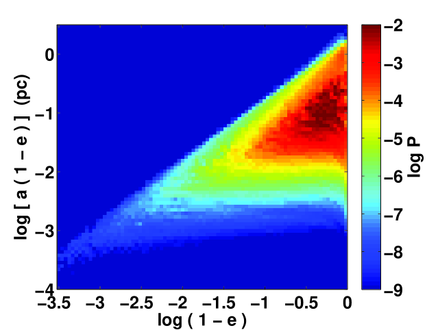
Figure 5: Two dimensional joint probability distribution ${\cal P}(r_{p},e)$ for the inner binary in the $[r_{p},e]$ plane (where $r_{p}=a(1-e)$). The distribution is obtained averaging over the 1000 3-body experiments described in Section 2.2

By knowing ${\cal F}_{t}$, we can write the coalescence rate of binaries that have experienced a triple interactions as ${\cal F}_{t}\times{d^{3}N/dzd{\cal M}dt_{r}}$. From the 3-body scattering presented in Section 2.2, we derive the joint probability distribution for the inner binary of having a certain periastron and a certain eccentricity, ${\cal P}(r_{p},e)$. This quantity is plotted in figure 5 for our set of the 1000 3-body realizations. This probability distribution refers to systems with mean total mass $\sim 4\times 10^{8}{\rm M}_{\odot}$. To extend it to a wider range of masses, we assume a triplet lifetime ${\cal T}=10^{9}$ yrs independently of the masses (which are in a narrow range peaked around $10^{8}{\rm M}_{\odot}$ in our case) and we rescale ${\cal P}(r_{p},e)$ so that, in the GW dominated regime, elements in the $(r_{p},e)$ space having the same coalescence timescale $T_{\rm gw}(r_{p},e)$, have the same probability value ${\cal P}(r_{p},e)$. Since $T_{\rm gw}\propto a^{4}/[M_{1}M_{2}(M_{1}+M_{2})]$, assuming an invariant binary mass ratio distribution in the relevant mass range (which is a good approximation given the narrow mass range we are dealing with), the $y$ axis in figure 5 is rescaled for any given total mass of the binary $M$ according to $(M/4\times 10^{8}{\rm M}_{\odot})^{3/4}$. We then compute the distribution of eccentric binaries emitting an observable burst as:

$$N({\cal M},z,r_{p},e) = \frac{d^{3}N}{dzd{\cal M}dt_{r}}\times{\cal F}_{t}\times{\cal T}\times{\cal P}(r_{p},e)\times$$

$$\times{\rm min}[1,(T_{\rm obs}/T_{\rm orb})].$$ (21)

Where the factor ${\rm min}[1,(T_{\rm obs}/T_{\rm orb})]$ takes into account the fact that if the binary period is longer than the observation time, only a fraction $T_{\rm obs}/T_{\rm orb}$ of the systems is actually bursting during the observation.

4.3 Practical computation of the signal

The relevant frequency band for pulsar timing observations is between $1/T_{\rm obs}$ and the Nyquist frequency $1/(2\Delta t)$ – where $\Delta t$ is the time between two adjacent observations–, corresponding to $3\times 10^{-9}$ Hz - $10^{-7}$ Hz. The frequency resolution bin is $\Delta f=1/T_{\rm obs}$, and we assume $T_{\rm obs}=10$ yr throughout the paper. Every realistic frequency–domain computation of the signal has to take into account the frequency resolution bin $\Delta f$ of the observation. The signal is therefore evaluated for discrete frequency bins $\Delta f_{j}$ centered at discrete values of the frequency $f_{j}$, where $f_{(j+1)}=f_{j}+\Delta f$. What we actually collect in our code is the numerical distribution $\Delta^{3}N/\Delta z\Delta{\cal M}\Delta f_{r}$, where $\Delta f_{r}=(1+z)\Delta f$. The integral in equation (18) is then replaced as a sum over redshift and chirp mass, and the value of the characteristic strain at each discrete frequency $f_{j}$ is computed as

$$h_{c}^{2}(f_{j})=\sum_{z}\sum_{{\cal M}}\,\frac{\Delta^{3}N}{\Delta z\Delta{\cal M}\Delta f_{r,j}}f_{r}\,h^{2}(z,{\cal M},f_{r}){\Delta z}{\Delta{\cal M}},$$ (22)

where $\Delta f_{r,j}=(1+z)\Delta f_{j}$ is the $j$th frequency bin shifted according to the cosmological redshift of the sources. Equation (22) is simply read as the sum of the squares of the characteristic strains of all the sources emitting in the observed frequency bin $\Delta f_{j}$. If we produce a family of $\alpha=1,...,K$ sources by performing a Monte Carlo sampling of the numerical distribution $\Delta^{3}N/\Delta z\Delta{\cal M}\Delta f_{r}$ of the emitting binary population, the characteristic strain is computed as

$$h_{c}^{2}(f_{j})=\sum_{\alpha=1}^{K}h_{c,\alpha}(z,{\cal M},f_{\alpha,r})^{2}\Theta[f_{\alpha,r},\Delta f_{j}(1+z)]$$ (23)

where $\Theta[f_{\alpha,r},\Delta f_{j}(1+z)]=1$ if $f_{\alpha,r}\in\Delta f_{j}(1+z)$ and is null elsewhere. To recover equation (22), the characteristic amplitude of the individual source is given by: $h_{c,\alpha}^{2}=h_{\alpha}^{2}f_{\alpha,r}/\Delta f_{r,j}\approx h_{\alpha}^{2}f_{j}/\Delta f_{j}=h_{\alpha}^{2}f_{j}T_{\rm obs}$; ı.e., the sky and polarization averaged amplitude square, multiplied by the number of cycles completed in the observation time. The induced rms residual of each individual source is then given by equation (12). Note that in the limit of large $K$ (formally, $K\rightarrow\infty$), $h_{c}(f_{j})$ computed according to equation (23) is independent of $T_{\rm obs}$ (because the increment of the contribution of each single source according to the number of cycles completed during $T_{\rm obs}$ is balanced by the fact that we sum over a frequency bin that is proportional to $1/T_{\rm obs}$), and its value coincides with the one obtained from the standard energy based definition of $h_{c}(f)$ (Sesana, Vecchio & Colacino, 2008). On the other hand, when $K$ is small (i.e. we sum over a small number of sources), fluctuations become important in the computation of the signal in each frequency bin. Numerical computation according to equation (23) allows us to account for signal fluctuations, which are missing in the analytical definition of the characteristic amplitude of the GW spectrum (e.g. Phinney, 2001), but are important in the actual computation of the observed signal. Given $h_{c}$, the induced rms timing residual produced by the whole emitting population is simply given by $h_{c}(f_{i})/(2\pi f_{i})$.

We generate a population of emitting binaries according to the numerical distribution $\Delta^{3}N/\Delta z\Delta{\cal M}\Delta f_{r}$, and we sum all the $h_{c,\alpha}$ contributions in every frequency bin to obtain the characteristic strain of the signal. We then generate, again using a Monte–Carlo sampling, a population of emitting eccentric binaries in triple systems from the distribution given in equation (21) and we compute their GW bursts and the induced rms residuals according to equations (9, 10, 13, 14). For the few systems reaching $10^{-5}$ Hz with their higher harmonics, we also compute the SNR produced in the LISA detector using equation (15), adopting the $S_{f}$ given in equation (48) of Barack & Cutler (2004), extended downward to $10^{-5}$ Hz as described in Section 3.1. We consider five different SMBH binary populations presented in SSV09 (Tu-SA, Tu-DA, Tu-NA, La-SA, Tr-SA) with two different fractions of triplets ${\cal F}_{t}=0.1,0.5$, for a grand total of 10 different models. We run 50 (when ${\cal F}_{t}=0.5$; 100 if ${\cal F}_{t}=0.1$) independent Monte–Carlo realizations of each single model, which allows us to perform a statistical study of the properties of the bursting sources. We consider only systems with $e>0.66$, because highly eccentric systems are those expected to burst at high frequencies, where the contribution of the overall circular binary population declines. And also because high eccentricities result in a well defined burst shape which may be essential to distinguish it from periodic sources.

5 Results

5.1 description of the signal

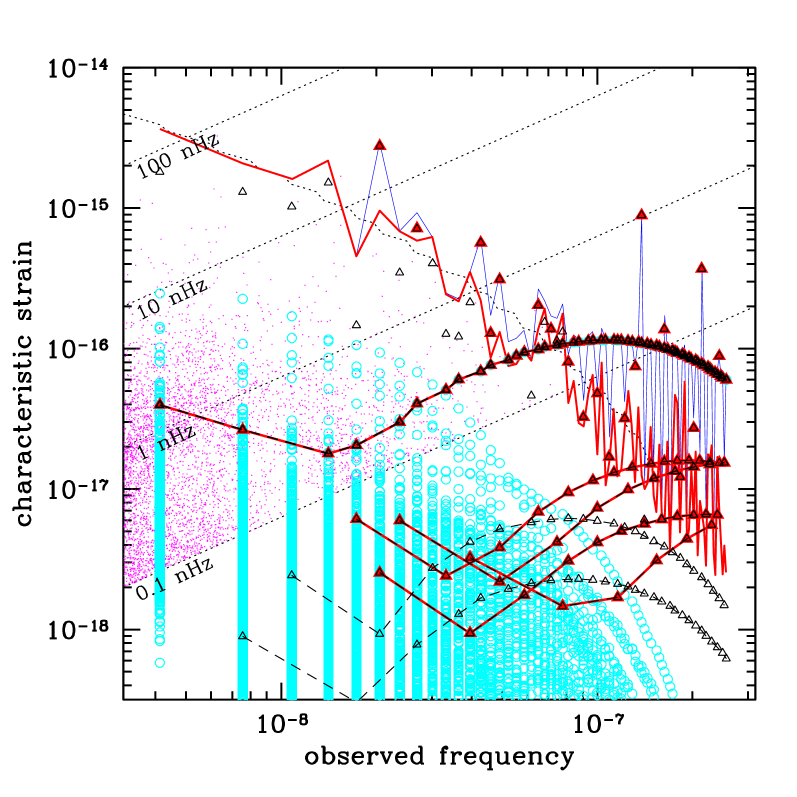
Figure 6: Representation of all the relevant features of a Monte–Carlo generated signal. The Tu-DA model with ${\cal F}=0.5$ is assumed. The jagged blue line is an individual Monte–Carlo realization of the signal. The small black triangles label the characteristic strain of the brightest source in each frequency bin. If the source is resolvable, it is also labeled with a big red triangle. The jagged red line is the stochastic level of the signal, i.e., once the resolvable sources in each frequency bin are subtracted. The magenta points label all the systems producing an rms residual (computed through equation (12)) larger than 0.1ns over 10 years. The cyan ’arcs’ of dots, represent the contribution to the signal coming from eccentric binaries in triple systems (bursting sources), again assuming that their total rms residual is larger than 0.1ns (equation (14)). The arc-like black (red) tracks represent the spectrum of the more luminous (resolvable) bursting systems in the realization, and have the only purpose of guiding the reader eye. The dotted oblique lines mark different rms residual levels as a function of the frequency.

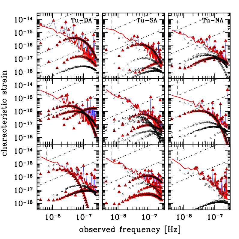
Figure 7: Sample of individual Monte–Carlo realizations of the signal generated using Tu-DA (left panels), Tu-SA (central panels) and Tu-NA (right panels) models (${\cal F}=0.5$). Line and point style as in figure 6. The two dashed lines in each panel represent the sensitivity of the PPTA (upper) survey and an indicative sensitivity of 1ns for SKA (lower).

All the relevant features of the signal are plotted in figure 6 for a realization of the Tu-DA model with ${\cal F}_{t}=0.5$. A Monte–Carlo generated signal is depicted as a blue jagged line. The magenta points represent all the binary systems producing a $\delta t_{\mathrm{gw}}>0.1$ ns; there are $\sim 4000$ sources in this particular realization. The cyan ’arcs’ of dots, represent the contribution to the signal coming from eccentric binaries in triple systems (bursting sources), where contributions from all harmonics falling in the same frequency bin were added in quadrature. The black triangles correspond to the brightest source in each frequency bin. And if a source is brighter than the sum of all the contributions coming from the other sources emitting in the same bin, we consider that source resolvable and we mark it with a superposed red triangle. The red jagged line is the resulting stochastic level of the signal, after the contribution from the resolvable sources has been subtracted. The arc-like black (red) tracks represent the more luminous (resolvable) bursting systems in the realization. In this particular case there were five resolvable bursts with rms residual $\delta t_{\rm gw}=3.5,0.07,0.04,0.01,0.002$ ns. However, considering realistic PTA sensitivities achievable in the near future ($\sim 1$ns, with the SKA), only the brightest one would have a good chance of being detected.

We note that we introduced the concept of resolvable source in the frequency domain, assuming that a source is resolvable if its strain is larger than the sum of the strains of all the other sources in that frequency bin. This definition is, however, only appropriate for monochromatic sources. A very eccentric burst, emitting a whole spectrum of harmonics, may not be the brightest source in any of the frequency bins, however, it may produce a significantly larger rms residuals with respect to other individual circular binaries. Moreover, in the time domain, the signature of these bursts is quite different with respect to periodic circular binaries, resulting in long bumps or narrow well localized bursts (see figure 10). Given these caveats, we will also present results in terms of total number of sources, independent of their resolvability according to our definition.

A sample of different realizations of the signal is collected in figure 7, for individual realizations of the three different Tu models. Only the brightest sources are plotted in this case. Given the small number of systems involved, their phenomenology is quite variable. For example, the realization illustrated in the left-middle panel, shows three resolvable bursts with $\delta t_{\rm gw}\gtrsim 3$ns; the one in the lower- left panel, does not show any individually resolvable bursts.

5.2 Statistic of bursting sources

Figure 8: Cumulative number $N(\delta t_{\mathrm{gw}})$ of circular binaries (thin lines) and bursting triplets (thick lines) emitting over a given $\delta{t_{\rm GW}}$ threshold as a function of $\delta{t_{\rm GW}}$. In each panels the different linestyles refer to the Tu-SA (solid), Tu-DA (long–dashed) and Tu-NA (short–dashed) models. The fraction of triplets assumed is labeled in each panel.

Figure 9: Same as figure 8, but considering only the resolvable sources in the computation of $N(\delta t_{\mathrm{gw}})$ according to equation (24). Linestyle as in figure 8.

To quantify the statistics of the bursting sources, we cast the results in terms of the cumulative number of sources as a function of the timing residuals:

$$N(\delta t_{\mathrm{gw}})=\int_{\delta t_{\mathrm{gw}}}^{\infty}\frac{dN}{d(\delta t_{\mathrm{gw}}^{\prime})}d(\delta t_{\mathrm{gw}}^{\prime})\,,$$ (24)

where the distribution $dN/d(\delta t_{\mathrm{gw}}^{\prime})$ is the average over the 50 (100) Monte–Carlo realizations of each model. We compute this average both considering all the sources emitting over a given $\delta t_{\mathrm{gw}}$ threshold (obtaining the total distribution of bursting sources), as well as considering only resolvable sources as defined in the previous section (obtaining the distribution of bursting resolvable sources). In figure 8, $N(\delta t_{\mathrm{gw}})$ for all the sources is shown. Depending on the adopted model, and on the fraction of triplets assumed, there are few hundred to few thousand binaries contributing to the signal at a level $\gtrsim 1$ns. The number of triplets over this threshold is between 20 and 60 assuming ${\cal F}=0.5$, and, not surprisingly, a factor of 5 lower if we assume ${\cal F}=0.1$. If triple interactions of SMBHs are common (say, ${\cal F}>0.1$), we may therefore expect 1-to-100 bursts from eccentric sources contributing to the GW signal at a residual level of $>1$ns. The eccentricity distribution of these bursts is basically flat in the considered eccentricity range $(0.66,1)$. If we consider resolvable sources only, the figures are not as promising. As shown in figure 9, a timing precision of 0.1 ns is needed to guarantee the detectability of a resolvable burst if ${\cal F}=0.5$. At a 1 ns level, we have less than one resolvable burst, we can then interpret the results in terms of the probability of having such bursts in our observable Universe. This probability ranges from 2% to 50% depending on the adopted model, and the eccentricity distribution of these resolvable events is biased towards high values, peaking around $e=0.9$. La-SA and Tr-SA give similar results both qualitatively and quantitatively, therefore we don’t plot them in the figures in order to keep them clear. Again, we stress the fact that our definition of resolvable source is rather arbitrary, and does not take into account for the peculiar shape of the burst, we then consider these figures as lower limits to the actual detectability of these bursts.

5.3 Signal samples in the time domain

To give a feeling of how the actual signals would appear, we also computed residuals in the time domain for selected sources. To this purpose, we evolved the system using equations (27)-(31) of Barack & Cutler (2004) assuming non spinning SMBHs. We then computed all the components $h_{+,n}$ and $h_{\times,n}$ (following Pierro, et al. 2001) and we finally evaluated the residuals $R(T)$ integrating equation (11). The actual shape of the residuals is rather complex and depends on the geometry of the system: the relative orientation of the source to the pulsars (encoded in the direction cosines $\alpha$, $\beta$, and $\gamma$ in equation (11)); the polarization angle of the source $\Psi$; the inclination $i$; the initial phase of the orbit $\Phi_{0}$; and an angle $\phi_{p}$ describing the orientation of the periastron in the orbital plane (see, e.g., Barack & Cutler 2004 for a definition of all these quantities).

Examples of the phenomenology of bursting sources are given in figure 10 for a sample of eccentric systems found in one selected realisation of the model Tu-DA. In the left panels we show the three brightest resolvable sources, while in the right panels we show three of the brightest bursts which would be unresolvable according to our definition, because their power spectra would be overwhelmed by the signal produced by the standard circular binaries found in the realization. Parameters of the binaries are given in table 2. Bursts can be generated by very eccentric-long period binaries (as in the two lower panels), or by relatively short-period systems (e.g., central left panel), in which case multiple bursts are visible in the observation times. The width of the burst depends on the periastron passage timescale: systems with $T_{p}\ll T_{\rm obs}$ produce narrow features in the data stream (e.g., lower left panel), while systems with $T_{p}\approx T_{\rm obs}$ give a characteristic bump shaping all over the data span (e.g. upper right panel). Given the integral nature of the signal (equation (11)), its shape is also heavily dependent on $\Phi_{0}$ (e.g. the cumulative residual can be positive or negative depending on the binary orbital phase at the beginning of the detection), on $\phi_{p}$ and on $\Psi$. The inclination of the source $i$ and its aperture angle to the pulsar, determine the amplitude of the signal.

Figure 10: Examples of timing residual, found in a particular realization of the model Tu-DA, computed according to equation (11). Different linestyles correspond to different aperture angle $\theta$ between the pulsar and the source; $\theta=\pi/2$ (dotted), $\pi/3$ (short–dashed), $\pi/6$ (long–dashed). In all the cases $\Psi=\pi/4$ and $i=\pi/3$. $\phi_{p}$ is random and $\Phi_{0}$ is chosen so that the burst occurs during the observation. The rms residual computed according to equation (14) are also shown. Parameters of the sources are listed in table 2.

$M_{1}$ [M⊙]	$M_{2}$ [M⊙]	$f_{r}$ [Hz]	$z$	$e$	$\delta t_{\rm gw}$[ns]
$1.4\times 10^{9}$	$4.4\times 10^{8}$	$1.92\times 10^{-10}$	0.965	0.232	6.82
$9.9\times 10^{8}$	$4.2\times 10^{7}$	$7.5\times 10^{-9}$	0.88	0.082	1.57
$9.8\times 10^{8}$	$3.9\times 10^{8}$	$1.38\times 10^{-10}$	0.979	0.775	2.11
$6.8\times 10^{8}$	$4.1\times 10^{8}$	$2.31\times 10^{-11}$	0.973	0.922	2.66
$1.2\times 10^{9}$	$4.1\times 10^{8}$	$4.03\times 10^{-10}$	0.84	0.239	9.84
$5.6\times 10^{9}$	$2.7\times 10^{8}$	$2.11\times 10^{-10}$	0.75	0.086	15.2

Table 2: Parameters of the sources plotted in figure 10. Rows in the table (from the top to the bottom), correspond to panels of figure 10 considered counterclockwise, starting from the upper left panel.

5.4 A note for LISA

We also collected catalogs of systems bursting in the LISA window, to check for detectability. Unfortunately, prospects for detection with LISA are not as promising as for PTAs. In a total of 750 realization of the ten different models, we found $\sim 50$ sources bursting in the LISA window producing an SNR$>0.1$. Unfortunately, none of them produced a SNR$>8$, necessary for a confident detection. We then conclude, that even with a consistent population of SMBH triplets forming during the cosmic history, burst from massive (say, ${\cal M}\sim 10^{8}{\rm M}_{\odot}$) eccentric binaries are unlikely to be produced at a significant rate for LISA. On the other hand, if formation of triple systems was common in the past, for system in the LISA mass range ($\sim 10^{5}-10^{7}{\rm M}_{\odot}$), very peculiar signals from coalescing eccentric binaries may be common in the data stream. However, this is beyond the scope of the present paper, where we focused on massive binaries (${\cal M}>10^{7}{\rm M}_{\odot}$) only.

6 Conclusions

We have addressed in this work three different points in the evolution of triplets of SMBHs in the Universe: The Astrodynamics of the system, the potential GW signature and the detectability.

We have performed eight different direct-summation $N-$body simulations, one including more than half a million of particles, to calibrate 1,000 3-body scattering experiments, which include post-Newtonian corrections, in order to have a statistical description of the system. Both numerical tools agree that the inner binary of SMBHs will go through a phase of extremely high eccentricity, which is the motivation for the rest of the work.

These three-body excitations of episodic high eccentricity configurations of the close SMBH binary produce interesting GW bursts that may be detectable with forthcoming experiments such as PTAs and LISA. The extreme eccentricities of such bursts on one hand would leave a very distinctive signature, but on the other require the development of appropriate analysis techniques.

To compute likely event rates, we extracted catalogues of merging galaxies from the Millennium Run, and we populated them with SMBHs following the known MBH-bulges relations. We then estimated the fractions of triplets and their eccentricity distribution and we computed the induced signals in both PTAs and the LISA detector.

We found that, depending on the details of the SMBH population model, if the fraction of triplets is $\geq 0.1$, few to a hundred of GW bursts would be produced at a $>1$ ns level in the PTA frequency domain. Most of the signals will be washed out in the confusion noise due to the emission of ‘ordinary’ low eccentric binaries. However, their peculiar features may guide the development of targeted data analysis techniques, that may help to recognize them even if overwhelmed by the confusion noise. Employing a minimal criterion for source resolvability (which provides a strict lower limit), we found that less than one system may be actually pinned down at ns precisions. By running several dozens of Monte Carlo realization of the signal from the cosmological population of SMBH binaries and triplets we quantified a statistical $2-50$% chance of having a resolvable burst in the Universe (assuming 10 yrs of observation). The probability for detection with LISA is essentially nil. However, we stress the fact that we focused on systems with ${\cal M}>10^{7}{\rm M}_{\odot}$; our results then simply imply that it is extremely unlikely that a system which would normally emit outside the LISA range will produce a burst in the LISA window because of resonant three body interactions. On the other hand, if a consistent fraction of light binaries (${\cal M}<10^{7}{\rm M}_{\odot}$) is involved in triple systems, we may expect several eccentricity-driven coalescences to be observed by LISA. This eventuality would call for the development of extremely eccentric templates ($e>0.9$) for merging SMBHs, and of adequate analysis techniques to extract the signal.

References

- Aarseth (1999) Aarseth, S. J., PASP 111, 1333, 1999
- Aarseth (2003a) Aarseth, S. J. 2003a, AAS, 285, 367
- Aarseth (2003b) Aarseth, S. J. 2003b, Gravitational N-Body Simulations, pp. 430. ISBN 0521432723. Cambridge, UK: Cambridge University Press, November 2003
- Amaro-Seoane & Spurzem (2001) Amaro-Seoane, P., & Spurzem, R. 2001, MNRAS, 327
- Amaro-Seoane & Freitag (2006) Amaro-Seoane, P.; Freitag, M., ApJ, 653, Issue 1, pp. L53-L56 (2006)
- Amaro-Seoane et al. (2007) Amaro-Seoane P., Gair J. R., Freitag M., Miller M. C., Mandel I., Cutler C. J., Babak S., 2007, Classical and Quantum Gravity, 24, 113
- Amaro-Seoane, Miller & Freitag (2009) Amaro-Seoane, P.; Miller, M. C.; Freitag, M., ApJ, 692, Issue 1, pp. L50-L53 (2009)
- Amaro-Seoane et al. (2009) Amaro-Seoane, P. and Eichhorn, C. and Porter, E. and Spurzem, R., 2009, accepted for publication in MNRAS, 2009
- Amaro-Seoane & Santamaria (2009) Amaro-Seoane, Pau; Santamaria, Lucia, ArXiv e-prints arXiv:0910.0254
- Barack & Cutler (2004) Barack L. & Cutler C., 2004, PhRvD, 082005
- Begelman, Blandford & Rees (1980) Begelman, M.C., Blandford, R.D., Rees, M.J. 1980, Nature 287, 307
- Bell et al. (2006) Bell E. F., Phleps S., Somerville R. S., Wolf C., Borch A. & Meisenheimer K., 2006, ApJ, 652, 270
- Bender et al. (1998) Bender P. L. et al., 1998 LISA Pre-Phase A Report; Second Edition, MPQ 233
- Berczik, et al. (2006) Berczik, P.; Merritt, D.; Spurzem, R.; Bischof, H.-P., 2006, ApJ, 642, L21
- Bertone, De Lucia & Thomas (2007) Bertone S., De Lucia G. & Thomas P. A., 2007, MNRAS, 379, 1143
- Bertotti, Carr & Rees (1983) Bertotti B., Carr B. J. & Rees M. J., 1983, MNRAS, 203, 945
- Detweiler (1979) Detweiler, S.L. 1979, ApJ, 234, 1100–1104
- Dotti et al. (2006a) Dotti, M., Colpi, M., & Haardt, F., 2006, MNRAS, 367, 103
- Escala et al. (2005) Escala, A., Larson, R. B., Coppi, P. S., & Mardones, D., 2005, ApJ, 630, 152
- Ferrarese & Merritt (2000) Ferrarese, L., Merritt, D. 2000, ApJ 539, L9
- Finn & Thorne (2000) Finn L. S. & Thorne K. S., 2000, PhRvD, 124021
- Frank & Rees (1976) Frank, J. & Rees, M. J. 1976, MNRAS, 176, 633
- Gebhardt, et al. (2000) Gebhardt, K., Richstone, D., Kormendy, J., Lauer, T.R., Ajhar, E.A., Bender, R., Dressler, A., Faber, S.M., Grillmair, C., Magorrian, J., Tremaine, S. 2000b, AJ 119, 1157
- Haehnelt & Kauffmann (2000) Haehnelt, M.G.; Kauffmann, G.: 2000, MNRAS, 318, L35.
- Hemsendorf, Sigurdsson, & Spurzem (2002) Hemsendorf, M., Sigurdsson, S., & Spurzem, R. 2002, ApJ, 581, 1256
- Hoffman & Loeb (2007) Hoffman, L. & Loeb, A., 2007, MNRAS, 377, 957
- Janssen et al. (2008) Janssen G.H. et al., 2008, in 40 YEARS OF PULSARS: Millisecond Pulsars, Magnetars and More. AIP, Conference Proceedings, Volume 983, 633
- Jenet et al. (2004) Jenet, F. A., Lommen, A., Larson, S. L., & Wen, L. 2004, ApJ, 606, 799
- Jenet et al. (2009) Jenet, F. A. et al., 2009, preprint (arXiv:0909.1058)
- Kauffmann & Haehnelt (2000) Kauffmann, G. & Haehnelt, M.G. 2000, MNRAS, 311, 576
- Kustaanheimo & Stiefel (1965) Kustaanheimo, P.E. & Stiefel, E. L. 1965, Publ. Astron. Obs. Helsinki 110, 204-219, J. Reine Angew. Math. 218, 204
- Lazio (2009) Lazio, J., 2009, arXiv:0910.0632
- Lin et al. (2008) Lin, L. et al., 2008, ApJ, 681, 232
- Makino & Ebisuzaki (1996) Makino, J. & Ebisuzaki, T. 1996, ApJ, 436, 607
- Manchester (2006) Manchester, R.N., 2006, Chin. J. Astron. Astrophys., 6, 139
- Manchester (2008) Manchester R.N., 2008, in 40 YEARS OF PULSARS: Millisecond Pulsars, Magnetars and More. AIP, Conference Proceedings, Volume 983, 584
- Merritt & Ferrarese (2001) Merritt, D. & Ferrarese, L. 2001, MNRAS, 320, L30
- Merritt & Poon (2004) Merritt, D. & Poon, M. Y., 2004, ApJ, 606, 788
- Mikkola & Aarseth (1990) Mikkola S. & Aarseth S., 1990, Celest. Mech. Dyn. Astron., 47, 375
- Mikkola & Aarseth (1993) Mikkola S. & Aarseth S., 1993, Celest. Mech. Dyn. Astron., 57, 439
- Milosavljević & Merritt (2001) Milosavljević, M. & Merritt, D. 2001, ApJ, 563, 34
- Milosavljević & Merritt (2003) Milosavljević, M. & Merritt, D. 2003, ApJ, 596, 860
- Peters & Mathews (1963) Peters, P.C. and Mathews, J. 1963, Phys. Rev., 131, 434–440
- Peters (1964) Peters, P.C., 1964, Phys. Rev., 136, 1224-1232
- Perets et al. (2007) Perets, H. B., Hopman, C., & Alexander, T., 2007, ApJ, 656, 709
- Phinney (2001) Phinney E. S., 2001, arXiv:astro-ph/0108028
- Pierro, et al. (2001) Pierro, V., Pinto, I.M., Spallicci, A.D., Laserra, E., & Recano, F. 2001, MNRAS, 325, 358–372
- Plummer (1911) Plummer H. C., 1911, MNRAS, 71, 460
- Pshirkov, Baskaran & Postnov (2009) Pshirkov M.S., Baskaran, D. & Postnov, K.A., 2009, arXiv:0909.0742
- Quinlan (1996) Quinlan, G. 1996, NewA, 1, 35.
- Richstone et al. (1998) Richstone, D. et al., 1998, Nature, 395, 14
- Sazhin (1978) Sazhin M. V., 1978, Soviet Astron., 22, 36
- Sesana et al. (2004) Sesana, A., Haardt, F., Madau, P., & Volonteri, M. 2004, ApJ, 611, 623.
- Sesana et al. (2005) Sesana A., Haardt F., Madau P. & Volonteri M., 2005, ApJ, 623, 23
- Sesana, Volonteri & Haardt (2007) Sesana A., Volonteri M. & Haardt F., 2007, MNRAS, 377, 1711
- Sesana, Vecchio & Colacino (2008) Sesana A., Vecchio A. & Colacino C. N., 2008, MNRAS, 390, 192
- Sesana, Vecchio & Volonteri (2009) Sesana A., Vecchio A. & Volonteri M., 2009, MNRAS, 394, 2255
- Springel et al. (2005) Springel V. et al., 2005, Nature, 435, 629
- Thorne (1987) Thorne, K. S. 1987, in 300 Years of Gravitation, ed. S. Hawking & W. Israel (Cambridge: Cambridge Univ. Press), 330
- Tremaine et al. (2002) Tremaine, S., et al. 2002, ApJ, 574, 740
- Tundo et al. (2007) Tundo E., Bernardi M., Hyde J. B., Sheth R. K. & Pizzella A., 2007, ApJ, 663, 57
- Valtonen, et al. (1994) Valtonen, M.J., Mikkola, S., Heinamaki, P., Valtonen, H. 1994, ApJS, 95, 69
- van Haasteren & Levin (2009) van Haasteren, R. & Levin, Y., 2009, arXiv:0909.0954
- Wyithe & Loeb (2003) Wyithe J. S. B. & Loeb A., 2003, ApJ, 590, 691
- Yu (2002) Yu, Q., 2002, MNRAS, 331, 935