Flavor-twisted boundary condition for simulations of quantum many-body systems

Abstract

We present an approximative simulation method for quantum many-body systems based on coarse graining the space of the momentum transferred between interacting particles, which leads to effective Hamiltonians of reduced size with the flavor-twisted boundary condition. A rapid, accurate, and fast convergent computation of the ground-state energy is demonstrated on the spin-$\frac{1}{2}$ quantum antiferromagnet of any dimension by employing only two sites. The method is expected to be useful for future simulations and quick estimates on other strongly correlated systems.

Understanding a quantum many-body system is fundamentally challenging because of the exponential growth of the number of states with the system size. To estimate the physical properties of an intractably large system, a common practice is to extrapolate the results for several significantly reduced sizes,Dagotto (1994) together with the periodic boundary condition (PBC).Ashcroft and Mermin (1976) A different yet complementary approach is to continuously twist the boundary conditions for one solvable size. The typical flavor-independent version of the latter has been seen in solid state physics,Poilblanc (1991); Tohyama (2004) while the flavor version has been used in quantum chromodynamics.de Divitiis et al. (2004); Sachrajda and Villadoro (2005); Tiburzi (2005) Here we apply the flavor-twisted boundary conditions (FTBC)de Divitiis et al. (2004); Sachrajda and Villadoro (2005); Tiburzi (2005) to the spin-$\frac{1}{2}$ quantum antiferromagnet, one of the basic models in solid state physics. We show that the ground-state energy can be accurately calculated using only two sites.

We begin with an explicit derivation of FTBC, which is necessary for systematical studies of this and related methods. Let us consider the connection between a large system of size $L$ and a small one of size $l$, both with PBC. (To distinguish them, the upper-case and lower-case letters are used thoroughly for the large and small lattices, respectively.) The large system is described by the following general Hamiltonian in the second quantized language and in the real space representation,

$$H_{L}=\sum_{\mathbf{I},\mathbf{J},\sigma}{(t_{\mathbf{I}\mathbf{J}}^{\sigma}C_{\mathbf{I}\sigma}^{\dagger}C_{\mathbf{J}\sigma}+h.c.})+\sum_{\begin{subarray}{c}\mathbf{I},\mathbf{J},\sigma\\ \mathbf{J}^{\prime},\mathbf{I}^{\prime},\sigma^{\prime}\end{subarray}}{U^{\sigma,\sigma^{\prime}}_{\mathbf{I}\mathbf{J}^{\prime}\mathbf{J}\mathbf{I}^{\prime}}C_{\mathbf{I}\sigma}^{\dagger}C_{\mathbf{J}^{\prime}\sigma^{\prime}}^{\dagger}C_{\mathbf{I}^{\prime}\sigma^{\prime}}C_{\mathbf{J}\sigma}},$$ (1)

where $C_{\mathbf{I}\sigma}$ denote the quantum operator that annihilates a particle with flavor $\sigma$ at site $\mathbf{I}$. $L=\prod_{\alpha=1}^{d}{L_{\alpha}}$ is the total number of the lattice sites in a $d$-dimensional space with $L_{\alpha}$ being the site number in the $\alpha$-dimension. The thermodynamic limit is reached when all $L_{\alpha}\to\infty$.

There also exists a reciprocal space where the counterpart of the site $\mathbf{I}$ is the momentum point $\mathbf{K}$. Imposing PBC to the real space discretizes the $\mathbf{K}$ space as follows Ashcroft and Mermin (1976)

$$K_{\alpha}=\frac{2\pi}{L_{\alpha}}M,\;\;\;M=0,1,2,\dots,L_{\alpha}-1$$ (2)

where all the lattice constants have been scaled to unit. Eq. (2) translates the concepts of large and small in the real space to those of fine and coarse in the $\mathbf{K}$ grid, respectively. In the reciprocal space,

$$H_{L}=\sum_{\mathbf{K}\sigma}{\varepsilon_{\mathbf{K}}^{\sigma}C_{\mathbf{K}\sigma}^{\dagger}C_{\mathbf{K}\sigma}}+\frac{1}{L}\sum_{\mathbf{Q}}\{\sum_{\mathbf{K}\sigma,\mathbf{K}^{\prime}\sigma^{\prime}}{U^{\sigma,\sigma^{\prime}}_{\mathbf{K},\mathbf{K}^{\prime},\mathbf{Q}}C_{\mathbf{K}+\mathbf{Q},\sigma}^{\dagger}C_{\mathbf{K}^{\prime}-\mathbf{Q},\sigma^{\prime}}^{\dagger}C_{\mathbf{K}^{\prime},\sigma^{\prime}}C_{\mathbf{K},\sigma}}\}$$ (3)

where $C_{\mathbf{K}\sigma}$ annihilates a particle with momentum $\mathbf{K}$ and spin $\sigma$ and is given by

$$C_{\mathbf{K}\sigma}=\frac{1}{\sqrt{L}}\sum_{\mathbf{I}}{e^{-i\mathbf{K}\cdot\mathbf{R}_{\mathbf{I}}}C_{\mathbf{I}\sigma}},$$ (4)

where $\mathbf{R}_{\mathbf{I}}$ is the coordinates of the $\mathbf{I}$-th site. The bare energy dispersion and the interaction function are

$$\varepsilon_{\mathbf{K}}^{\sigma} = \sum_{\mathbf{R}_{\mathbf{J}}-\mathbf{R}_{\mathbf{I}}}t_{\mathbf{I}\mathbf{J}}^{\sigma}e^{i\mathbf{K}\cdot(\mathbf{R}_{\mathbf{J}}-\mathbf{R}_{\mathbf{I}})}.$$ (5)

$$U^{\sigma,\sigma^{\prime}}_{\mathbf{K},\mathbf{K}^{\prime},\mathbf{Q}} = \sum_{\begin{subarray}{c}\mathbf{R}_{\mathbf{J}}-\mathbf{R}_{\mathbf{I}}\\ \mathbf{R}_{\mathbf{I}^{\prime}}-\mathbf{R}_{\mathbf{J}^{\prime}}\\ \mathbf{R}_{\mathbf{J}^{\prime}}-\mathbf{R}_{\mathbf{I}}\end{subarray}}U^{\sigma,\sigma^{\prime}}_{\mathbf{I}\mathbf{J}^{\prime}\mathbf{J}\mathbf{I}^{\prime}}e^{i\mathbf{K}\cdot(\mathbf{R}_{\mathbf{J}}-\mathbf{R}_{\mathbf{I}})}e^{i\mathbf{K}^{\prime}\cdot(\mathbf{R}_{\mathbf{I}^{\prime}}-\mathbf{R}_{\mathbf{J}^{\prime}})}e^{i\mathbf{Q}\cdot(\mathbf{R}_{\mathbf{J}^{\prime}}-\mathbf{R}_{\mathbf{I}})}.$$ (6)

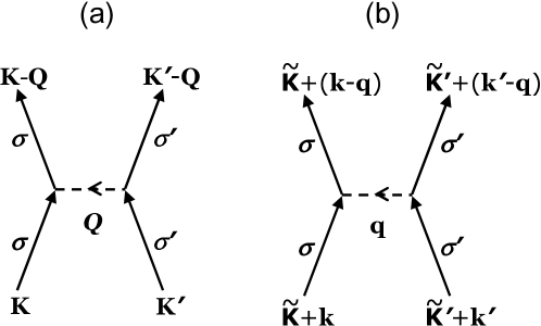
Figure 1: Illustration of the momentum transfer due to the particle-particle interaction: (a) original and (b) coarsened.

Eq. (3) appears to describe two particles with $\mathbf{K}$ and $\mathbf{K}^{\prime}$, respectively, interact with internal momentum transfer $\mathbf{Q}$, as diagrammed in Fig. 1(a). Since the $\mathbf{Q}$ points are to be integrated [c.f. $\sum_{\mathbf{Q}}\{\cdots\}$ in Eq. (3)], here comes a well-known numerical trick: the summation (integration) over a fine grid may be well approximated by that over a rather coarse grid. This numerical recipe receives particular support in the quantum many-body systems of interest, where a small number of $\mathbf{Q}$ are far more important than the others, the so-called $\mathbf{Q}$-mode resonance, e.g., $\mathbf{Q}=(\pi,\pi,\cdots,\pi)$ in antiferromagnetic correlation. The $\mathbf{Q}$-mode resonance implies dramatic response to small stimuli such as changing temperature, applied fields, pressure, doping, etc, which is important to determining the functionalities of the system. Therefore, it may be a good approximation to coarsen the $\mathbf{Q}$ grid as long as the important $\mathbf{Q}$ points are included.

To find a way to coarsen the $\mathbf{Q}$ grid such that the resulting Hamiltonian can be readily transformed back to the real space (where the parameters are often short-ranged, meriting for numerical computation), we consider the small system of size $l$ with PBC whose momenta $\mathbf{k}$ are given by:

$$k_{\alpha}=\frac{2\pi}{l_{\alpha}}m,\;\;\;m=0,1,2,\dots,l_{\alpha}-1.$$ (7)

where $l=\Pi_{\alpha=1}^{d}{l_{\alpha}}\ll L$ is the total site number of the smaller lattice. Let the small system be commensurate with the large one, that is, all the $\mathbf{k}$ points can be found in the $\mathbf{K}$ grid of the large system. Then, any momentum in the fine $\mathbf{K}$ grid can be rewritten as,

$$\mathbf{K}=\tilde{\mathbf{K}}+\mathbf{k},\;\;\;\;\mathbf{K}^{\prime}=\tilde{\mathbf{K}}^{\prime}+\mathbf{k}^{\prime},\;\;\;\;\mathbf{Q}=\tilde{\mathbf{Q}}+\mathbf{q},$$ (8)

where $\mathbf{k}^{\prime}$ and $\mathbf{q}$ are in the $\mathbf{k}$ grid defined in Eq. (7); the $L/l$ ‘twists’ $\tilde{\mathbf{K}}$ (likewise $\tilde{\mathbf{K}}^{\prime}$ or $\tilde{\mathbf{Q}}$) consist of a subset of the original $\mathbf{K}$ points that fill the interstitial region of the $\mathbf{k}$ points nearby the origin. For example, for $d=1$,

$$\tilde{K}_{\alpha}\in(-\frac{\pi}{l_{\alpha}},\frac{\pi}{l_{\alpha}}].$$ (9)

As another example, $l=2$ for the square lattice means that $\mathbf{k}=(0,0)$ and $(\pi,\pi)$, and that $\tilde{\mathbf{K}}$ cover half of the original $\mathbf{K}$ space satisfying $\cos(\tilde{K}_{x})+\cos(\tilde{K}_{y})\geq 0$.

One can explicitly rewrite $H_{L}$ in terms of the real-space $l$-site lattice by introducing a new set of particle annihilation operators,

$$d_{\mathbf{k}\sigma;\tilde{\mathbf{K}}}=C_{\tilde{\mathbf{K}}+\mathbf{k}\sigma}=C_{\mathbf{K}\sigma},$$ (10)

$$d_{\mathbf{i}\sigma;\tilde{\mathbf{K}}}=\frac{1}{\sqrt{l}}\sum_{\mathbf{k}}{e^{i\mathbf{k}\cdot\mathbf{r}_{i}}d_{\mathbf{k}\sigma;\tilde{\mathbf{K}}}},$$ (11)

where $\mathbf{r}_{i}$ is the coordinates of the $i$-th site of this $l$-site lattice, satisfying

$$\sum_{\mathbf{k}}e^{i\mathbf{k}\cdot(\mathbf{r}_{\mathbf{j}}-\mathbf{r}_{\mathbf{i}})}=l\delta_{\mathbf{i},\mathbf{j}}.$$ (12)

By using Eqs. (7-12), the original Hamiltonian for the $L$-site system, Eq. (1) or Eq. (3), can be transformed to a set of $l$-site subsystems described by the following new Hamiltonian in the real space representation

$$H_{L} = \sum_{\tilde{\mathbf{K}}\sigma}\sum_{\mathbf{i},\mathbf{j}}[e^{i\tilde{\mathbf{K}}\cdot(\mathbf{r}_{j}-\mathbf{r}_{i})}t_{\mathbf{ij}}^{\sigma}d_{\mathbf{i}\sigma;\tilde{\mathbf{K}}}^{\dagger}d_{\mathbf{j}\sigma;\tilde{\mathbf{K}}}+h.c.]+\frac{l}{L}\sum_{\tilde{\mathbf{Q}}}\;\sum_{\tilde{\mathbf{K}}\sigma,\tilde{\mathbf{K}}^{\prime}\sigma^{\prime}}\;\sum_{\mathbf{i},\mathbf{i}^{\prime},\mathbf{j},\mathbf{j}^{\prime}}$$ (13)

$${\left\{e^{i\tilde{\mathbf{K}}\cdot(\mathbf{r}_{j}-\mathbf{r}_{i})}e^{i\tilde{\mathbf{K}}^{\prime}\cdot(\mathbf{r}_{i^{\prime}}-\mathbf{r}_{j^{\prime}})}e^{i\tilde{\mathbf{Q}}\cdot(\mathbf{r}_{j^{\prime}}-\mathbf{r}_{i})}U_{\mathbf{i}\mathbf{j}^{\prime}\mathbf{j}\mathbf{i}^{\prime}}^{\sigma,\sigma^{\prime}}d_{\mathbf{i}\sigma;\tilde{\mathbf{K}}+\tilde{\mathbf{Q}}}^{\dagger}d_{\mathbf{j}^{\prime}\sigma^{\prime};\tilde{\mathbf{K}}^{\prime}-\tilde{\mathbf{Q}}}^{\dagger}d_{\mathbf{i}^{\prime}\sigma^{\prime};\tilde{\mathbf{K}}^{\prime}}d_{\mathbf{j}\sigma;\tilde{\mathbf{K}}}\right\}}.$$

This establishes the exact transformation between the large and the small, subject to the linear size of the small system being not shorter than the range of any Hamiltonian parameters of Eq. (1).

Approximation 1.—Now we coarse the $\mathbf{Q}$ grid with

$$\tilde{\mathbf{Q}}\equiv 0.$$ (14)

This means that only the $\mathbf{q}$ points, whose total number is $l$, are retained as the internal momentum transfer. Then, $\mathbf{K}+\mathbf{q}=\tilde{\mathbf{K}}+\mathbf{k}+\mathbf{q}=\tilde{\mathbf{K}}+\mathbf{k}^{\prime}$. That is, any $\mathbf{K}$ point is scattered to the sum of the same twist and another point in $\{\mathbf{q}\}$. Thus, a particle with a given $\tilde{\mathbf{K}}$ can be scattered by the particle-particle interaction into only $l$ points in the $\mathbf{K}$ momentum space, instead of $L$ points, as illustrated in Fig. 1(b). Eq. (13) is rewritten as

$$H_{L}\simeq\frac{l}{L}\sum_{\tilde{\mathbf{K}}\sigma,\tilde{\mathbf{K}}^{\prime}\sigma^{\prime}}H_{l}({\tilde{\mathbf{K}}\sigma,\tilde{\mathbf{K}}^{\prime}\sigma^{\prime}}),$$ (15)

where the subsystems are

$$H_{l}({\tilde{\mathbf{K}}\sigma,\tilde{\mathbf{K}}^{\prime}\sigma^{\prime}}) = \sum_{\mathbf{i},\mathbf{j}}[e^{i\tilde{\mathbf{K}}\cdot(\mathbf{r}_{j}-\mathbf{r}_{i})}t_{\mathbf{ij}}^{\sigma}d_{\mathbf{i}\sigma;\tilde{\mathbf{K}}}^{\dagger}d_{\mathbf{j}\sigma;\tilde{\mathbf{K}}}+h.c.]+$$ (16)

$$+\sum_{\mathbf{i},\mathbf{j}}[e^{i\tilde{\mathbf{K}}^{\prime}\cdot(\mathbf{r}_{j}-\mathbf{r}_{i})}t_{\mathbf{ij}}^{\sigma^{\prime}}d_{\mathbf{i}\sigma^{\prime};\tilde{\mathbf{K}}^{\prime}}^{\dagger}d_{\mathbf{j}\sigma^{\prime};\tilde{\mathbf{K}}^{\prime}}+h.c.]+$$

$$+\sum_{\mathbf{i},\mathbf{j},\mathbf{j}^{\prime},\mathbf{i}^{\prime}}{e^{i\tilde{\mathbf{K}}\cdot(\mathbf{r}_{j}-\mathbf{r}_{i})}e^{i\tilde{\mathbf{K}}^{\prime}\cdot(\mathbf{r}_{i^{\prime}}-\mathbf{r}_{j^{\prime}})}U_{\mathbf{i}\mathbf{j}^{\prime}\mathbf{j}\mathbf{i}^{\prime}}^{\sigma,\sigma^{\prime}}d_{\mathbf{i}\sigma;\tilde{\mathbf{K}}}^{\dagger}d_{\mathbf{j}^{\prime}\sigma^{\prime};\tilde{\mathbf{K}}^{\prime}}^{\dagger}d_{\mathbf{i}^{\prime}\sigma^{\prime};\tilde{\mathbf{K}}^{\prime}}d_{\mathbf{j}\sigma;\tilde{\mathbf{K}}}}.$$

Combined with Eq. (15), Eq. (16) for each pair of $\tilde{\mathbf{K}}$ and $\tilde{\mathbf{K}}^{\prime}$ is not independent of another pair. For example, the {$\tilde{\mathbf{K}}$, $\tilde{\mathbf{K}}^{\prime}$} subsystem and the {$\tilde{\mathbf{K}}$, $\tilde{\mathbf{K}}^{\prime\prime}$} subsystem share the same momentum points with $\tilde{\mathbf{K}}$. Therefore, all the $(L/l)^{2}$ subsystems of size $l$ are connected and one still has to deal with a case of size $L$. To simplify the calculations to size $l$, a further approximation is needed.

Approximation 2 (FTBC).—A simple approximation is to treat $H_{l}({\tilde{\mathbf{K}}\sigma,\tilde{\mathbf{K}}^{\prime}\sigma^{\prime}})$ independently. Thus, to estimate the expectation value of an observable $\hat{O}_{L}$ in the large system is to calculate

$$\mathrm{trace}(\hat{\rho}_{L}\,\hat{O}_{L})\simeq\sum_{\tilde{\mathbf{K}}\sigma,\tilde{\mathbf{K}}^{\prime}\sigma^{\prime}}\mathrm{trace}(\hat{\rho}_{l;{\tilde{\mathbf{K}}\sigma,\tilde{\mathbf{K}}^{\prime}\sigma^{\prime}}}\,\hat{O}_{l;{\tilde{\mathbf{K}}\sigma,\tilde{\mathbf{K}}^{\prime}\sigma^{\prime}}}),$$ (17)

where $\hat{\rho}_{L}$ denotes the density matrix for the large system and $\hat{\rho}_{l;{\tilde{\mathbf{K}}\sigma,\tilde{\mathbf{K}}^{\prime}\sigma^{\prime}}}$ denotes the density matrix for the isolated small system with the twists $\tilde{\mathbf{K}}$ and $\tilde{\mathbf{K}}^{\prime}$, as determined by Eq. (16). $\hat{O}_{l;{\tilde{\mathbf{K}}\sigma,\tilde{\mathbf{K}}^{\prime}\sigma^{\prime}}}$ is the transformed observable following Eqs. (10)-(12) and Eq. (14). For example, the ground state energy is approximated by

$$\langle\Phi_{L}|\sum_{\tilde{\mathbf{K}}\sigma,\tilde{\mathbf{K}}^{\prime}\sigma^{\prime}}H_{l}({\tilde{\mathbf{K}}\sigma,\tilde{\mathbf{K}}^{\prime}\sigma^{\prime}})|\Phi_{L}\rangle\simeq\sum_{\tilde{\mathbf{K}}\sigma,\tilde{\mathbf{K}}^{\prime}\sigma^{\prime}}\langle\phi_{l;{\tilde{\mathbf{K}}\sigma,\tilde{\mathbf{K}}^{\prime}\sigma^{\prime}}}|H_{l}({\tilde{\mathbf{K}}\sigma,\tilde{\mathbf{K}}^{\prime}\sigma^{\prime}})|\phi_{l;{\tilde{\mathbf{K}}\sigma,\tilde{\mathbf{K}}^{\prime}\sigma^{\prime}}}\rangle,$$ (18)

where $|\Phi_{L}\rangle$ denotes the ground-state wave function for the large system and $|\phi_{l;{\tilde{\mathbf{K}}\sigma,\tilde{\mathbf{K}}^{\prime}\sigma^{\prime}}}\rangle$ denotes a wave function for the isolated small system with the twists $\tilde{\mathbf{K}}$ and $\tilde{\mathbf{K}}^{\prime}$.

This approximation is actually equivalent to FTBC (Ref. Tiburzi, 2005) as explained below. Comparing Eq. (16) with Eq. (1), one finds that they are very similar in form—only differ in the parameters by a phase factor $e^{i\tilde{\mathbf{K}}\cdot(\mathbf{r}_{i}-\mathbf{r}_{j})}$ associated with the momentum twist $\tilde{\mathbf{K}}$. Actually, solving Eq. (16) is equivalent to solving the following Hamiltonian for the $l$-site lattice

$$H_{l}({\tilde{\mathbf{K}}\sigma,\tilde{\mathbf{K}}^{\prime}\sigma^{\prime}}) = \sum_{\mathbf{i},\mathbf{j}}{(t_{\mathbf{ij}}^{\sigma}d_{\mathbf{i}\sigma;\tilde{\mathbf{K}}}^{\dagger}d_{\mathbf{j}\sigma;\tilde{\mathbf{K}}}+h.c.)}+\sum_{\mathbf{i},\mathbf{j}}{(t_{\mathbf{ij}}^{\sigma^{\prime}}d_{\mathbf{i}\sigma^{\prime};\tilde{\mathbf{K}}^{\prime}}^{\dagger}d_{\mathbf{j}\sigma^{\prime};\tilde{\mathbf{K}}^{\prime}}+h.c.)}$$ (19)

$$+\sum_{\mathbf{i},\mathbf{j},\mathbf{j}^{\prime},\mathbf{i}^{\prime}}{U_{\mathbf{i}\mathbf{i}^{\prime}\mathbf{j}\mathbf{j}^{\prime}}^{\sigma,\sigma^{\prime}}d_{\mathbf{i}\sigma;\tilde{\mathbf{K}}}^{\dagger}d_{\mathbf{i}^{\prime}\sigma^{\prime};\tilde{\mathbf{K}}^{\prime}}^{\dagger}d_{\mathbf{j}^{\prime}\sigma^{\prime};\tilde{\mathbf{K}}^{\prime}}d_{\mathbf{j}\sigma;\tilde{\mathbf{K}}}}$$

together with the boundary conditions such that translating its many-body wavefunction $|\Psi_{l}\rangle$ along the $\alpha$-th dimension $l_{\alpha}$ steps yield $e^{i(N_{1}\tilde{K}_{\alpha}+N_{2}\tilde{K}^{\prime}_{\alpha})l_{\alpha}}|\Psi_{l}\rangle$ where $N_{1}$ and $N_{2}$ are the numbers of the two flavors of particles associated with the two twists $\tilde{\mathbf{K}}$ and $\tilde{\mathbf{K}}^{\prime}$, respectively.

With FTBC, the problem of solving the original Hamiltonian for a $L$-site system is reduced to solving $(L/l)^{2}$ Hamiltonians for $l$-site subsystems, each corresponding to a given pair of $\tilde{\mathbf{K}}$ and $\tilde{\mathbf{K}}^{\prime}$. The computational benefit is substantial, since the number of states grows exponentially with the system size. For the Hubbard model as an example, the calculation load is reduced from $O(4^{L}4^{L})$ to $O[(L/l)^{2}\times 4^{l}4^{l}]$. In addition, the $(L/l)^{2}$ prefactor is fully parallelizable and it can be readily handled by using the same integration trick of replacing a fine-grid sum with a coarse-grid sum. Since FTBC is reached at the level of Hamiltonian and interpreted as boundary conditions, it has least limitation and fully compatible with other many-body approaches, e.g., Lanczos exact diagonalization and quantum Monte Carlo methods.Dagotto (1994)

Approximation 3.—The typical twisted boundary conditionsPoilblanc (1991); Tohyama (2004) (TBC) can be reached from Eqs. (15) and (16) by further taking the $\tilde{\mathbf{K}}=\tilde{\mathbf{K}}^{\prime}$ approximation,

$$\frac{l}{L}\sum_{{\tilde{\mathbf{K}}\sigma,\tilde{\mathbf{K}}^{\prime}\sigma^{\prime}}}H_{l}({\tilde{\mathbf{K}}\sigma,\tilde{\mathbf{K}}^{\prime}}\sigma^{\prime})\approx\sum_{{\tilde{\mathbf{K}}\sigma,\sigma^{\prime}}}H_{l}(\tilde{\mathbf{K}}\sigma,\tilde{\mathbf{K}}\sigma^{\prime}).$$ (20)

With TBC, each subsystem has only one momentum twist $\tilde{\mathbf{K}}$. Commonly, the one-site or two-site ($\mathbf{r}_{i^{\prime}}=\mathbf{r}_{i}$ and $\mathbf{r}_{j^{\prime}}=\mathbf{r}_{j}$) interactions are the leading interaction terms. Then, the twisted phases of the interaction terms in Eq. (16) cancel, which renders the interaction terms for $l$ to be of the same form as those for $L$. Thus, the approximation by TBC allows the continuous sampling of the momentum space for one-particle excitations, but it prohibits the same for two-particle excitations. To compare, FTBC allows both in principle. It could be expected that FTBC is more accurate, as illustrated below.

To complete, PBC is an additional approximation of TBC ($\tilde{\mathbf{K}}=\tilde{\mathbf{K}}^{\prime}=0$). FTBC with one twist zero fixed ($\tilde{\mathbf{K}}^{\prime}=0$, referred to as FTBC0)de Divitiis et al. (2004); Sachrajda and Villadoro (2005) was studied before.

To illustrate all the above points, we use FTBC to estimate the ground state energy of the spin-1/2 Heisenberg quantum antiferromagnet of any dimension. Here the flavor is the spin of electrons, consisting of $\uparrow$ and $\downarrow$.spi The results are compared with those obtained from using the other boundary conditions and linear spin-wave theory (LSW).Anderson (1952)

The spin-1/2 antiferromagnetic Heisenberg model is given by

$$H_{L}=J\sum_{\langle\mathbf{I},\mathbf{J}\rangle}{[S_{\mathbf{I}}^{z}S_{\mathbf{J}}^{z}+\frac{1}{2}(S_{\mathbf{I}}^{+}S_{\mathbf{J}}^{-}+S_{\mathbf{I}}^{-}S_{\mathbf{J}}^{+})]},$$ (21)

where the spin operator $S_{\mathbf{I}}^{+,-,z}=\sum_{\mu\nu}{C_{\mathbf{I}\mu}^{\dagger}\sigma^{+,-,z}_{\mu\nu}C_{\mathbf{I}\nu}}$ with $\sigma^{+,-,z}_{\mu\nu}$ being the Pauli matrix elements. $\sum_{\langle\mathbf{I},\mathbf{J}\rangle}$ runs over nearest neighbors. It is not only the basic account of antiferromagnetism Mattis (1981) but also the ground zero of understanding high-temperature superconductivity in copper oxides.Manousakis (1991); Anderson (1987) Two interesting states have been intensively considered in the literature: the long-range ordered Néel state and the resonating-valence-bond (RVB) state.Anderson (1987, 1973) The concept of RVB is based on the fact that the minimum bond energy ($-0.75J$) is realized in a two-site system, much lower than the bond energy ($-0.25J$) of the classic Néel state; the valence-bond between two nearest-neighbor spins is arguably key to understanding low-dimensional quantum antiferromagnets.Anderson (1973) However, the 2-site dimer breaks bonding to spins on the other sites in an extended system. For example, the total energy from the dimers is $-0.375J$ per bond for $d=1$ and $-0.1875J$ per bond for $d=2$, much higher than the exact result Bethe (1931); Hulthén (1938) $-0.443J$ for $d=1$ and the numerical result Huse (1988) $-0.334J$ for $d=2$, respectively. It is argued that the resonating (i.e., superposition of the degenerate states of different dimer configurations) could lower the energy substantially.Anderson (1973) But an accurate estimation of the ground state energy was achieved only when long-distance spin dimers were also included.Liang et al. (1988)

With FTBC, after coarsening the $\mathbf{Q}$ mesh, one obtains

$$H_{l}({\tilde{\mathbf{K}}_{\uparrow},\tilde{\mathbf{K}}_{\downarrow}})=J\sum_{\langle\mathbf{i},\mathbf{j}\rangle}\{{s_{\mathbf{i}}^{z}s_{\mathbf{j}}^{z}}+\frac{1}{2}[e^{i(\tilde{\mathbf{K}}_{\uparrow}-\tilde{\mathbf{K}}_{\downarrow})\cdot(\mathbf{r}_{j}-\mathbf{r}_{i})}s_{\mathbf{i}}^{+}s_{\mathbf{j}}^{-}+h.c.]\},$$ (22)

where $s_{\mathbf{i}}^{+}=d_{\mathbf{i}\uparrow;\tilde{\mathbf{K}}\uparrow}^{\dagger}d_{\mathbf{i}\downarrow;\tilde{\mathbf{K}}\downarrow}$, $s_{\mathbf{i}}^{-}=d_{\mathbf{i}\downarrow;\tilde{\mathbf{K}}\downarrow}^{{\dagger}}d_{\mathbf{i}\uparrow;\tilde{\mathbf{K}}\uparrow}$ and $s_{\mathbf{i}}^{z}=\frac{1}{2}(d_{\mathbf{i}\uparrow;\tilde{\mathbf{K}}\uparrow}^{\dagger}d_{\mathbf{i}\uparrow;\tilde{\mathbf{K}}\uparrow}-d_{\mathbf{i}\downarrow;\tilde{\mathbf{K}}\downarrow}^{\dagger}d_{\mathbf{i}\downarrow;\tilde{\mathbf{K}}\downarrow})$. The spin-exchange terms strongly depend on the double twists, $\tilde{\mathbf{K}}_{\uparrow}$ and $\tilde{\mathbf{K}}_{\downarrow}$, for the spin-up and spin-down electrons, respectively. In comparison, the result with TBC is

$$H_{l}(\tilde{\mathbf{K}}_{\uparrow},\tilde{\mathbf{K}}_{\downarrow})=J\sum_{\mathbf{i},\mathbf{j}}\{{s_{\mathbf{i}}^{z}s_{\mathbf{j}}^{z}}+\frac{1}{2}(s_{\mathbf{i}}^{+}s_{\mathbf{j}}^{-}+s_{\mathbf{i}}^{-}s_{\mathbf{j}}^{+})\},$$ (23)

independent of twists, the same as with PBC in this case.

The accuracy and convergency of FTBC are tested with the bond energy

$$E({L;l})=\frac{1}{n_{\mathrm{bond}}}\left(\frac{l}{L}\right)^{2}\sum_{\tilde{\mathbf{K}}_{\uparrow},\tilde{\mathbf{K}}_{\downarrow}}\langle H_{l}(\tilde{\mathbf{K}}_{\uparrow},\tilde{\mathbf{K}}_{\downarrow})\rangle,$$ (24)

where $n_{\mathrm{bond}}$ is the number of the nearest-neighbor AF bonds in the small system. Let us first take the most dramatic approximation, viz: $l=2$ (note $n_{\mathrm{bond}}=1$), the fundamental of the RVB state. With PBC, the $\mathbf{q}$ mesh contains only two points: $(0,0,\dots,0)$ and $(\pi,\pi,\dots,\pi)$ corresponding to a spin singlet and a triplet, respectively; the energy of the $\mathbf{q}=0$ state is $-0.75J$. By using FTBC to continuously and smoothly twist the energies of the subsystems, the bond energy becomes

$$E(L;l=2) = J\left(\frac{2}{L}\right)^{2}\sum_{\tilde{\mathbf{K}}_{\uparrow},\tilde{\mathbf{K}}_{\downarrow}}{[-\frac{1}{4}-\frac{1}{2}e^{i(\tilde{\mathbf{K}}_{\uparrow}-\tilde{\mathbf{K}}_{\downarrow})\cdot(\mathbf{r}_{1}-\mathbf{r}_{0})}]}$$ (25)

$$= -\frac{J}{4}-\frac{J}{2}\prod_{\alpha=1}^{d}\frac{1}{(2\pi)^{2}}\int_{-\pi}^{\pi}\mathrm{d}\tilde{K}^{\alpha}_{\uparrow}\int_{-\pi}^{\pi}\mathrm{d}\tilde{K}^{\alpha}_{\downarrow}{\cos(\tilde{K}^{\alpha}_{\uparrow}/2)\cos(\tilde{K}^{\alpha}_{\downarrow}/2)}$$

$$= -\frac{J}{4}-\frac{J}{2}\left(\frac{2}{\pi}\right)^{2d}\;\;\mathrm{for}\;L\to\infty.$$

The results are listed in Table 1, together with those obtained from using FTBC0, TBC, and PBC as well as the LSW results. The bond energy in the thermodynamic limit and for any dimension is accurately reproduced using the simple Eq. (25) for $l=2$.

Table 1: The ground-state energy per bond (in unit of $J$) of the spin-1/2 Heisenberg quantum antiferromagnet in the thermodynamic limit for the linear chain ($d=1$), the square lattice ($d=2$), and the body-centered-cubic lattice ($d=3$). The results from using FTBC, FTBC0, TBC or PBC are calculated with $l=2$.

Methods	$d=1$	$d=2$	$d=3$	$d=\infty$
exact/best known	$-0.443$	$-0.334$	$-0.288$	$-0.250$
LSW	$-0.432$	$-0.329$	$-0.287$	$-0.250$
FTBC	$-0.453$	$-0.332$	$-0.283$	$-0.250$
FTBC0	$-0.568$	$-0.453$	$-0.379$	$-0.250$
TBC (=PBC)	$-0.750$	$-0.750$	$-0.750$	$-0.750$

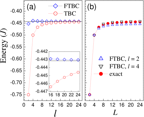
Figure 2: (a) Bond energy of the one-dimensional spin-1/2 Heisenberg antiferromagnet for $L\to\infty$ estimated from using FTBC (diamonds) and TBC or PBC (circles) for a number of $l$. The horizontal solid line denotes the exact solution ($-J\ln 2+J/4$). The dotted lines are guide to eyes. (b) Bond energy of the one-dimensional spin-1/2 Heisenberg antiferromagnet for a number of $L$ estimated from using FTBC for $l=2$ and $4$ (triangles), respectively, compared with the exact solutions (circles).

Next, the convergency of the bond energy $E(L\to\infty;l)$ with respect to $l$ is presented in Fig. 2(a). The energy of each subsystem is calculated with the Lanczos exact diagonalization method and a 5-point Gaussian integration in the twist momentum space, which is enough for the 6-digit accuracy. It is obvious that the estimate from FTBC converges to the exact solution $-J\ln 2+J/4$ (Refs. Bethe, 1931 and Hulthén, 1938) much faster than the extrapolation to $L\to\infty$ from finite-size scaling of the PBC or TBC results. Finally, $E(L;2)$ and $E(L;4)$ for a number of $L$ are plotted in Fig.  2(b) and compared with the exact solutions for $L$ in order to show the fast convergence of FTBC with respect to the size of the simulated system. Overall, the errors for $l=4$ are smaller than for $l=2$ ($0.003$ versus $0.009$ for $L=24$). For $l=2$, the small deviations from the exact solutions for $L\geq 4$ follow a power law $-0.009510(5)+0.152(2)/L^{1.976(6)}$ with $\chi^{2}=1.7326\times 10^{-11}$. This means that the error grows rather slowly as $L$ increases away from $l$. These results indicate that a large-scale feature of a quantum antiferromagnet could be captured at the length scale of one lattice constant with FTBC.

Finally, it is worth mentioning that in the above derivation of FTBC, we have revealed a less approximated approach, i.e., Eq. (14) alone. It is interesting to explore this approach and compare it with FTBC. Also, the explicit formulation of FTBC could facilitate to devise other approximations with lighter computational load. These studies are beyond the scope of the present work and will be published elsewhere.

Summarizing, based on coarse graining the space of the momentum transferred between interacting particles, we have derived the flavor-twisted boundary condition for simulating quantum many-body systems with effective Hamiltonians of reduced size. A rapid, accurate, and fast convergent computation of the ground-state energy is demonstrated on the spin-$\frac{1}{2}$ quantum antiferromagnet of any dimension by employing only two sites. The method is expected to be useful for future simulations and quick estimates on other strongly correlated systems.

W.Y. is grateful to P. D. Johnson and T. Valla for collaborations valla that stimulated this work. This research utilized resources at the New York Center for Computational Sciences at Stony Brook University/Brookhaven National Laboratory which is supported by the U.S. Department of Energy under Contract No. DE-AC02-98CH10886 and by the State of New York.

References

• Dagotto (1994) E. Dagotto, Rev. Mod. Phys. 66, 763 (1994).
• Ashcroft and Mermin (1976) N. W. Ashcroft and N. D. Mermin, Solid State Physics (Harcourt Brace, New York, 1976), p. 135.
• Poilblanc (1991) D. Poilblanc, Phys. Rev. B 44, 9562 (1991).
• Tohyama (2004) T. Tohyama, Phys. Rev. B 70, 174517 (2004).
• de Divitiis et al. (2004) G. de Divitiis, R. Petronzio, and N. Tantalo, Phys. Lett. B 595, 408 (2004).
• Sachrajda and Villadoro (2005) C. Sachrajda and G. Villadoro, Phys. Lett. B 609, 73 (2005).
• Tiburzi (2005) B. C. Tiburzi, Phys. Lett. B 617, 40 (2005).
• (8) The standard models with interaction between electrons of different spins also include the Hubbard, $t$-$J$, Anderson, and Kondo models.
• Anderson (1952) P. W. Anderson, Phys. Rev. 86, 694 (1952).
• Mattis (1981) D. C. Mattis, The Theory of Magnetism I (Springer-Verlag, Berlin, 1981).
• Manousakis (1991) E. Manousakis, Rev. Mod. Phys. 63, 1 (1991).
• Anderson (1987) P. W. Anderson, Science 235, 1196 (1987).
• Anderson (1973) P. W. Anderson, Mat. Res. Bull. 8, 153 (1973).
• Bethe (1931) H. Bethe, Z. Phys. 71, 205 (1931).
• Hulthén (1938) L. Hulthén, Ark. Met. Astron. Fysik 26A, Na. 11 (1938).
• Huse (1988) D. A. Huse, Phys. Rev. B 37, 2380 (1988).
• Liang et al. (1988) S. Liang, B. Doucot, and P. W. Anderson, Phys. Rev. Lett. 61, 365 (1988).
• Betts et al. (1998) D. D. Betts, J. Schulenburg, G. E. Stewart, J. Richter, and J. S. Flynn, J. Phys. A: Math. Gen. 31, 7685 (1998).
• (19) T. Valla, T. E. Kidd, W.-G. Yin, G. D. Gu, P. D. Johnson, Z.-H. Pan, and A.V. Fedorov, Phys. Rev. Lett. 98, 167003 (2007).