The landscape of quantum transitions driven by single-qubit unitary transformations with implications for entanglement

Abstract

This paper considers the control landscape of quantum transitions in multi-qubit systems driven by unitary transformations with single-qubit interaction terms. The two-qubit case is fully analyzed to reveal the features of the landscape including the nature of the absolute maximum and minimum, the saddle points, and the absence of traps. The results permit calculating the Schmidt state starting from an arbitrary two-qubit state following the local gradient flow. The analysis of multi-qubit systems is more challenging, but the generalized Schmidt states also may be located by following the local gradient flow. Finally, we show the relation between the generalized Schmidt states and the entanglement measure based on the Bures distance.

This is an author-created, un-copyedited version of an article accepted for publication in J. Phys. A: Math. Theor. IOP Publishing Ltd is not responsible for any errors or omissions in this version of the manuscript or any version derived from it. The definitive publisher authenticated version is available online at 10.1088/1751-8113/42/27/275303

1 Introduction

The topology of quantum control landscapes is important because it establishes the general features of the control behavior generated by applying external fields [1, 2]. The landscape for quantum transitions, assuming complete controllability, was analysed with the conclusion that there are no traps [3, 4, 5, 6] that could hinder achieving the highest possible control outcome. This paper studies the problem of describing the landscape of quantum transitions driven by local unitary operators, i.e., those acting on one qubit at a time, for multi-qubit systems [7].

The Schmidt states, defined for pure bi-partite systems, are important because of the insight they can provide about entanglement. The Schmidt states were generalized in [8, 9], in order to treat multipartite systems. This paper will show how to obtain the canonical form of the generalized Schmidt states by following the local gradient flow. This technique ultimately leads to a method to measure the entanglement of pure systems based on the optimal implementation of local unitary operations as a subset of the more general classical operations and classical communication protocols as it was pursued with other methods [10, 11].

It is convenient to define the following bracket operation

$$\langle X\rangle_{0} = \frac{1}{2N}Tr[X+X^{\dagger}]$$ (1)

The comparative fidelity between two density matrices, when at least one of them is pure is $\langle\rho_{0}\rho_{T}\rangle_{0}$. If one of the states is driven by a unitary operator, then the cost function can be written as

$$F=\langle U^{\dagger}\rho_{0}U\rho_{T}\rangle_{0},$$ (2)

This expression has the same form as the cost function for the optimization of the expectation value of an observable $\mathcal{O}$ [5],

$$\mathcal{J}_{1}=\langle U\rho_{0}U^{\dagger}\mathcal{O}\rangle_{0},$$ (3)

which was the subject of prior landscape studies [2]. The fidelity function for the state transfer can be rewritten as

$$F=\langle\rho_{0}U\rho_{T}U^{\dagger}\rangle_{0}.$$ (4)

An infinitesimal transformation of the unitary operator can be expressed as

$$U\rightarrow U^{\prime}=Ue^{\delta A}=U(1+\delta A),$$ (5)

with $\delta A$ being an anti-Hermitian element that lies in the corresponding Lie algebra, so that an infinitesimal variation of $U$ becomes

$$\delta U=U\delta A,$$ (6)

which can be used to calculate the first order variation of the fidelity as

$$\delta F=\langle\rho_{0}U[\delta A,\rho_{T}]U^{\dagger}\rangle_{0}.$$ (7)

A subsequent manipulation results in

$$\delta F=\langle[\rho_{T},U^{\dagger}\rho_{0}U]\delta A\rangle_{0}=\langle[\rho_{T},U^{\dagger}\rho_{0}U]U^{\dagger}\delta U\rangle_{0}$$ (8)

thereby identifying the gradient as

$$Grad_{1}=U[U^{\dagger}\rho_{0}U,\rho_{T}],$$ (9)

with the corresponding gradient flow equation

$$\frac{dU}{ds}=U[U^{\dagger}\rho_{0}U,\rho_{T}].$$ (10)

The fidelity can be expanded up to second order to obtain the quadratic form for the Hessian

$$\delta^{2}F=\langle\{\rho_{T},U^{\dagger}\rho_{0}U\}(\delta A)^{2}\rangle_{0}-2\langle U^{\dagger}\rho_{0}U\delta A\rho_{T}\delta A\rangle_{0},$$ (11)

where $\{,\}$ stands for the anti-commutator. This quadratic form is simplified at the critical points where the gradient (10) is zero

$$\delta^{2}F|_{c}=2(\langle\rho_{T}U^{\dagger}\rho_{0}U(\delta A)^{2}\rangle_{0}-\langle U^{\dagger}\rho_{0}U\delta A\rho_{T}\delta A\rangle_{0}).$$ (12)

The local gradient flow is found by eliminating multi-qubit terms in $\delta A$, such as $\sigma_{3}\otimes\sigma_{3}$ and leaving single qubit terms, such as $\sigma_{3}\otimes\mathbf{1}_{2\times 2}$ or $\mathbf{1}_{2\times 2}\otimes\sigma_{3}$. In this way, only strictly localized interactions are involved as happens in classical mechanics. Defining $\mathcal{P}$ as the projector that eliminates multi-qubit terms, the variation of the unitary operator with the corresponding local flow is

$$\delta U=U\mathcal{P}\delta A.$$ (13)

The projector $\mathcal{P}$ is easily calculated by tracing one-qubit terms. For example, the two-qubit projector is

$$\mathcal{P}=\frac{1}{4}\sum_{j=1}^{3}Tr[\,\cdot\,\,\sigma_{0}\otimes\sigma_{j}]\sigma_{0}\otimes\sigma_{j}+Tr[\,\cdot\,\,\sigma_{j}\otimes\sigma_{0}]\sigma_{j}\otimes\sigma_{0},$$ (14)

with $\sigma_{0}=\mathbf{1}_{2\times 2}$, so that $\mathcal{P}\delta A$ is constrained to the six-dimensional Lie algebra $su(2)\times su(2)\subset su(4)$. The first order variation subject to the local flow becomes

$$\delta F=\langle[\rho_{T},U^{\dagger}\rho_{0}U]\mathcal{P}U^{\dagger}\delta U\rangle_{0}=\langle\mathcal{P}\left([\rho_{T},U^{\dagger}\rho_{0}U]\right)U^{\dagger}\delta U\rangle_{0},$$ (15)

which results in the following local gradient

$$Grad_{1}^{local}=U\mathcal{P}[U^{\dagger}\rho_{0}U,\rho_{T}].$$ (16)

2 Two-Qubit Systems

The Schmidt states play an important role in the quantification of the entanglement of two-qubit systems. We will show their importance in describing the quantum landscape characterized by the local gradient flow and then calculate the Schmidt state of a given entangled state by following the local gradient flow (excepting the maximally entangled state).

Consider the landscape where the target state is a Schmidt state denoted as $\rho_{T}=\rho_{S}(\theta)$. The Schmidt states for two-qubit systems can be parametrized with a single variable as

$$|\psi_{\rho_{S}}\rangle=\cos(\theta/2)|\uparrow\uparrow\,\rangle+\sin(\theta/2)|\downarrow\downarrow\,\rangle,$$ (17)

whose corresponding density matrix reads

$$\rho_{S}(\theta)=\begin{pmatrix}\cos^{2}(\theta/2)&0&0&\frac{1}{2}\sin\theta\\ 0&0&0&0\\ 0&0&0&0\\ \frac{1}{2}\sin\theta&0&0&\sin^{2}(\theta/2)\end{pmatrix},$$ (18)

with $0\leq\theta\leq\pi$, in the standard basis $\{|\uparrow\uparrow\,\rangle,|\uparrow\downarrow\,\rangle,|\downarrow\uparrow\,\rangle,|\downarrow\downarrow\,\rangle\}$.

The critical states $\rho_{c}=U_{c}^{\dagger}\rho_{0}U_{c}$ obey the following equation

$$\mathcal{P}[\rho_{c},\rho_{S}(\theta)]=0$$ (19)

It can be shown that this equation is satisfied by critical states that fall into one of the following two cases

• Another Schmidt state $\rho_{c}=\rho_{S}(\phi)$. In this case, the eigenvalues of the Hessian around the critical points are either negative or mixed, with the following explicit form

  $$h(\theta,\phi)=\begin{pmatrix}0\\ -1-\cos(\theta-\phi)-\sin\theta-\sin\phi\\ -1-\cos(\theta-\phi)-\sin\theta-\sin\phi\\ -4\sin\theta\sin\phi\\ -1-\cos(\theta-\phi)+\sin\theta+\sin\phi\\ -1-\cos(\theta-\phi)+\sin\theta+\sin\phi\end{pmatrix},$$ (20)

  For each critical state with a negative spectrum $h(\theta_{0},\phi_{0})$, there is another one with a mixed spectrum $h(\theta_{0},\pi-\phi_{0})$. Conversely, for each critical state with a mixed spectrum $h(\theta_{0},\phi_{0})$, there is another one with a negative spectrum $h(\theta_{0},\pi-\phi_{0})$. So, for each initial state there is a pair of critical states that can be reached by following the local gradient flow, such that one of them is a saddle point and the other is an stable maximal point. If the initial state is separable, the two possible critical states are given by $\rho_{S}(0)$ or $\rho_{S}(\pi)$.

• The critical sub-manifold spanned by the basis $\{|\uparrow\downarrow\,\rangle,|\downarrow\uparrow\,\rangle\}$ with the following explicit form of the critical state

  $$\rho_{c}=x|\downarrow\uparrow\,\rangle\langle\downarrow\uparrow|+(1-x)|\uparrow\downarrow\,\rangle\langle\uparrow\downarrow|,$$ (21)

  where the eigenvalues of the Hessian are

  $$\begin{pmatrix}1-\sqrt{(1-2x)^{2}\cos^{2}\theta+\sin^{2}\theta}\\ 1-\sqrt{(1-2x)^{2}\cos^{2}\theta+\sin^{2}\theta}\\ 0\\ 1+\sqrt{(1-2x)^{2}\cos^{2}\theta+\sin^{2}\theta}\\ 1+\sqrt{(1-2x)^{2}\cos^{2}\theta+\sin^{2}\theta}\\ 0\end{pmatrix},$$ (22)

  which corresponds to a positive spectrum, associated with the minimum.

Based on the features of the critical points we can state the following theorem

Theorem 1

The fidelity landscape between a pure separable state $\rho_{0}$ and a target Schmidt state $\rho_{S}(\theta)$ (with $\theta\neq\pi/2$) has saddle points but no traps. Moreover, the separable states that maximize the fidelity converge to either $|\uparrow\uparrow\,\rangle$ or $|\downarrow\downarrow\,\rangle$ depending on the target state as they follow the local gradient flow, according to the following formula

$$\lim_{U\rightarrow U_{c}}{U^{\dagger}\rho_{0}U}=\begin{cases}|\uparrow\uparrow\,\rangle\langle\uparrow\uparrow|&0<\theta<\pi/2\\ |\downarrow\downarrow\,\rangle\langle\downarrow\downarrow|&\pi/2<\theta<\pi\end{cases},$$ (23)

This theorem is a direct result of the fact that those limiting states are the only Schmidt states with zero entanglement. Moreover, we can also say that

Corollary 1

For pure states, the maximum fidelity between an entangled state and a separable state can be calculated from the corresponding Schmidt state $|\psi_{S}\rangle=\cos(\theta/2)|\uparrow\uparrow\,\rangle+\sin(\theta/2)|\downarrow\downarrow\,\rangle$ as

$$\mathcal{F}(\theta)=\max F=\begin{cases}\cos^{2}(\theta/2)&\theta\leq\pi/2\\ \sin^{2}(\theta/2)&\pi/2<\theta\leq\pi\end{cases}$$ (24)

The maximum fidelity $\mathcal{F}(\theta)$ can be used to calculate the Bures distance as the entanglement measure, which satisfies all the features required for a good entanglement monotone [12, 13]. In the present case of pure two-qubit systems the entanglement formula is

$$E_{B}(\rho)=2\left(1-\sqrt{\mathcal{F}(\theta}\right).$$ (25)

As a first example, Figure 1 shows the fidelity of the states following the local gradient flow for the initial separable state described by

$$\rho_{0}=e^{\frac{i}{4\pi}\sigma_{0}\otimes\sigma_{1}}|\uparrow\uparrow\,\rangle\langle\uparrow\uparrow|e^{-\frac{i}{4\pi}\sigma_{0}\otimes\sigma_{1}}$$ (26)

with $\rho_{S}(\pi/4)$ as the target state and $|\uparrow\uparrow\,\rangle$ as the limiting state.

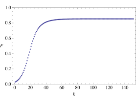
Figure 1: Fidelity curve of the states following the local gradient flow for the initial separable state (26) with $\rho_{S}(\pi/4)$ as the target state. The fidelity never reaches 1 but attains the global maximum associated with the limiting state $|\uparrow\uparrow\,\rangle$.

The next example considers the following entangled initial state

$$\rho_{0}=e^{\frac{i}{\pi/4}\sigma_{2}\otimes\sigma_{0}}e^{\frac{7i}{10\pi}\sigma_{2}\otimes\sigma_{2}}|\uparrow\uparrow\,\rangle\langle\uparrow\uparrow|e^{-\frac{7i}{10\pi}\sigma_{2}\otimes\sigma_{2}}e^{-\frac{i}{\pi/4}\sigma_{2}\otimes\sigma_{0}}$$ (27)

driven by the local unitary flow with $\rho_{S}(\pi/4)$ as the target state, and the following limiting Schmidt state

$$\lim_{U\rightarrow U_{c}}{U^{\dagger}\rho_{0}U}=\begin{pmatrix}0.793893&0&0&0.404508\\ 0&0&0&0\\ 0&0&0&0\\ 0.404508&0&0&0.206107\end{pmatrix}.$$ (28)

Almost any Schmidt state can be used as the target state in order to drive the local gradient flow, excepting those with $\theta=\{0,\pi/2,\pi\}$, because of convergence issues. For example, Figure 2 shows how the arbitrary state (27) approaches its Schmidt state for the range of target Schmidt states.

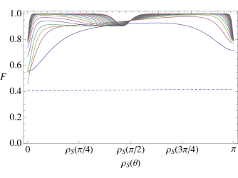
Figure 2: Fidelity of a random entangled state moving towards its Schmidt state as a function of the target Schmidt state $\rho_{S}(\theta)$ employed to drive the local gradient flow. The dashed line represents the fidelity of the initial random state with respect to its Schmidt state and each subsequent curve corresponds to another step in the approach by following the local gradient flow. The figure suggests that the arbitrary state never reaches its corresponding Schmidt state when the gradient employs the target states $\rho_{S}(0)$, $\rho_{S}(\pi/2)$ and $\rho_{S}(\pi)$.

The local gradient flow was driven by employing target Schmidt states, but the landscape is invariant under the application of local unitary operations on both the initial and target state. The local unitary transformations include local phases, that are able to change the phase of the Schmidt states. This means that the general stable critical states are Schmidt states with the possibility of extra phases. For example, consider the following arbitrary entangled state made from a Schmidt state and local unitary transformations

$$\rho_{E}=e^{\frac{i\pi}{4}\sigma_{2}\otimes\sigma_{0}}e^{\frac{i\pi}{4}\sigma_{0}\otimes\sigma_{1}}\rho_{S}(\pi/4)e^{-\frac{i\pi}{4}\sigma_{0}\otimes\sigma_{1}}e^{-\frac{i\pi}{4}\sigma_{2}\otimes\sigma_{0}}.$$ (29)

The initial separable state is taken as $\rho_{i}=|\uparrow\uparrow\,\rangle\langle\uparrow\uparrow|$. The local gradient flow converges to a separable unitary operator $U_{c}$ with the following corresponding separable state

$$\rho_{c}=U_{c}^{\dagger}\rho_{i}U_{c}=\begin{pmatrix}1/2&-1/2\\ -1/2&1/2\end{pmatrix}\otimes\begin{pmatrix}1/2&-i/2\\ i/2&1/2\end{pmatrix}.$$ (30)

This state can be diagonalized by the following local unitary operator

$$T=\begin{pmatrix}1/\sqrt{2}&1/\sqrt{2}\\ -1/\sqrt{2}&1/\sqrt{2}\end{pmatrix}\otimes\begin{pmatrix}i/\sqrt{2}&i/\sqrt{2}\\ -1/\sqrt{2}&1/\sqrt{2}\end{pmatrix},$$ (31)

such that $T^{\dagger}\rho_{c}T=|\uparrow\uparrow\,\rangle\langle\uparrow\uparrow|$. This suggests that $T$ could be used to reduce $\rho_{E}$ to its expected Schmidt state $\rho_{S}(\pi/4)$, but instead we obtain a Schmidt state with an extra phase $-i$

$$T^{\dagger}\rho_{E}T=\begin{pmatrix}\cos^{2}\left(\frac{\pi}{8}\right)&0&0&-i\cos\left(\frac{\pi}{8}\right)\sin\left(\frac{\pi}{8}\right)\\ 0&0&0&0\\ 0&0&0&0\\ i\cos\left(\frac{\pi}{8}\right)\sin\left(\frac{\pi}{8}\right)&0&0&\sin^{2}\left(\frac{\pi}{8}\right)\end{pmatrix}.$$ (32)

This extra phase can be eliminated by the use of local phase transformations, which otherwise leave the absolute value of the components of the density matrix invariant.

3 Three or More Qubit Systems

The entanglement in a two-qubit system can be minimally characterized by a single variable as shown in the Schmidt state. The number of variables needed to parametrize a n-qubit system is $2^{n+1}-2$ up to a global phase, and the number of variables to parametrize a single qubit is $3n$, thus, the minimum number of variables needed to parametrize the entanglement of an n-qubit system is

$$N_{E}=2^{n+1}-2-3n,$$ (33)

which is five for three-qubit systems. The canonical form of the generalized Schmidt states is important because of the information that can be obtained about entanglement [14, 15, 16, 14]. A canonical form of the generalized Schmidt state for three-qubits was introduced in [8] as

$$|\psi_{S}\rangle=\lambda_{1}|\uparrow\uparrow\uparrow\rangle+\lambda_{2}e^{i\phi}|\uparrow\downarrow\downarrow\rangle+\lambda_{3}|\downarrow\uparrow\downarrow\rangle+\lambda_{4}|\downarrow\downarrow\uparrow\rangle+\lambda_{5}|\downarrow\downarrow\downarrow\rangle,$$ (34)

with $\lambda_{i}\geq 0$, $\phi\geq 0$ and $\sum|\lambda_{i}|^{2}=1$. The canonical form of the generalized Schmidt state for n-qubit systems was given in [9] indicating that the missing basis elements in the generalized Schmidt state are

$$|\downarrow\uparrow\uparrow...\uparrow\rangle,|\uparrow\downarrow\uparrow...\uparrow\rangle,|\uparrow\uparrow\downarrow...\uparrow\rangle,...|\uparrow\uparrow\uparrow...\downarrow\rangle.$$ (35)

The landscape of multi-qubit systems is richer and more complex than the two-qubit case. Considering the case where the initial state is separable and following the reasoning in [9], we can always demand that $\lambda_{1}\geq\lambda_{k}$. However, the analysis is simpler if we relax some generality and demand that $\lambda_{1}>\lambda_{k}$, for $k>1$. The variation of the fidelity can be written as

$$\delta F=\delta\langle\Psi|\psi_{S}\rangle\langle\psi_{S}|\Psi\rangle=2Re[\langle\Psi|\psi_{S}\rangle\langle\psi_{S}|\delta|\Psi\rangle]$$ (36)

The canonical form in (34) indicates that if we start with a generic separable state $|\Psi\rangle=|\psi_{1}\rangle\otimes|\psi_{2}\rangle\otimes|\psi_{3}\rangle$ and allow local unitary transformations, the isolated maximum fidelity is achieved at the critical state $|\Psi_{c}\rangle=|\uparrow\uparrow\uparrow\,\rangle$. The first order variation under local unitary transformations is made of a linear combination of basis elements with at most one qubit reversed,

$$\delta|\uparrow\uparrow\uparrow\rangle=(1+i\delta_{1})|\uparrow\uparrow\uparrow\rangle+\delta_{2}|\downarrow\uparrow\uparrow\rangle+\delta_{3}|\uparrow\downarrow\uparrow\rangle+\delta_{5}|\uparrow\uparrow\downarrow\rangle,$$ (37)

with $\delta_{1}\in\mathbb{R}$, $\delta_{2}\in\mathbb{C}$, $\delta_{3}\in\mathbb{C}$, $\delta_{5}\in\mathbb{C}$. We can use this variation in order to evaluate $\delta F$ given by (36) at the critical state $|\Psi_{c}\rangle$ and verify that it is a stationary point, thus justifying the canonical form of the generalized Schmidt state. The missing basis elements (35) form a critical sub-manifold associated with the fidelity minimum of zero value. The generic identification of the remaining critical states is difficult and depends on the specific $\lambda_{j}$ values. However, if $\lambda_{j}>0$, then there are no additional critical states because the aforementioned critical states exhaust all the possibilities to obtain $\delta F=0$.

As a concrete example, consider calculating the generalized Schmidt state of the following arbitrary state

$$|\psi_{T}\rangle=\begin{pmatrix}0.3+0.1i\\ 0.2\\ 0.3\\ 0.3\\ 0.4\\ 0.2\\ 0.5\\ \sqrt{1-0.77}\end{pmatrix}.$$ (38)

Following the same procedure used in the two-qubit case, we use the local gradient flow to calculate the optimized separable state $|\psi_{c}\rangle$ that maximizes the fidelity $|\langle\psi_{T}|\psi_{c}\rangle|^{2}$, starting form an initial separable state (e.g. $|\uparrow\uparrow\uparrow\,\rangle$). The optimized state $|\psi_{c}\rangle$ can be diagonalized using a local unitary transformation. Applying the same local unitary transformation to the target state $|\psi_{T}\rangle\langle\psi_{T}|$ we obtain

$$|\hat{\psi}_{S}\rangle=\begin{pmatrix}0.986657\\ 0\\ 0\\ -0.125609-0.0245643i\\ 0\\ 0.0151643-0.0312796i\\ 0.0703562+0.0477398i\\ -0.0138602+0.0387071i\end{pmatrix},$$ (39)

which is almost in the canonical form (34). The first component can always be put in real form by choosing a suitable global phase. The remaining procedure is to employ the three available local phase transformations in order to eliminate the phase of last three components to finally obtain

$$|\psi_{S}\rangle=\begin{pmatrix}0.986657\\ 0\\ 0\\ -0.125609-0.0245643i\\ 0\\ 0.0347616\\ 0.085024\\ 0.0411138\end{pmatrix},$$ (40)

which we ascertain to be the global maximum because $|\lambda_{1}|$ is greater than the rest of the components. The local phase transformations do not change the absolute value of the components of the column spinor, so, it is easy to verify that, for example, in the last component $|-0.0138602+0.0387071i|=0.0411138$.

The procedure to calculate the Schmidt state can be used to calculate the Bures distance as an entanglement measure if $|\lambda_{1}|$ is greater than the rest of the components. In this case the formula of the Bures distance as a measure of entanglement is simply

$$E_{B}(\rho)=2(1-|\lambda_{1}|).$$ (41)

The study of higher multi-qubit states follows along the same general lines of the three-qubit state. Thus, we are able to calculate the generalized Schmidt state as well as the Bures distance as a measure of entanglement for most of the cases where $\lambda_{1}$ results in a value greater than the rest of the components.

4 Conclusions

The landscape of local quantum transitions for two-qubit systems is well suited for optimization through the gradient flow because of the lack of traps. We showed how to extend these results to muli-qubit systems and presented an example on how to calculate the generalized Schmidt state for three-qubits. The local gradient flow can be easily applied to higher multi-qubit systems and even though we could not give a complete analysis of the landscape, a criteria was presented to establish if the global maximum was attained. A generalization of this analysis to mixed multi-qubits is desireable, but this is a much more challenging problem because of the severe limitations that unitary transformations present.

References

References

- [1] Anthony P. Peirce, Mohammed A. Dahleh, and Herschel Rabitz. Optimal control of quantum-mechanical systems: Existence, numerical approximation, and applications. Phys. Rev. A, 37(12):4950–4964, Jun 1988.
- [2] Raj Chakrabarti and Herschel Rabitz. Quantum control landscapes. International Reviews in Physical Chemistry, 26(4):671–735, 2007.
- [3] H. Rabitz, M.M. Hsieh, and C.M. Rosenthal. Quantum Optimally Controlled Transition Landscapes. Science, 303(5666):1998–2001, 2004.
- [4] H. Rabitz. Controlling quantum phenomena: Why does it appear easy to achieve? Journal of Modern Optics, 51(16):2469–2475, 2004.
- [5] H. Rabitz, M. Hsieh, and C. Rosenthal. Optimal control landscapes for quantum observables. The Journal of Chemical Physics, 124:204107, 2006.
- [6] H. Rabitz, T.S. Ho, M. Hsieh, R. Kosut, and M. Demiralp. Topology of optimally controlled quantum mechanical transition probability landscapes. Physical Review A, 74(1):12721, 2006.
- [7] T. Schulte-Herbrueggen, SJ Glaser, G. Dirr, and U. Helmke. Gradient Flows for Optimisation and Quantum Control: Foundations and Applications. eprint arXiv: 0802.4195, 2008.
- [8] A. Acín, A. Andrianov, L. Costa, E. Jané, J. I. Latorre, and R. Tarrach. Generalized schmidt decomposition and classification of three-quantum-bit states. Phys. Rev. Lett., 85(7):1560–1563, Aug 2000.
- [9] H. A. Carteret, A. Higuchi, and A. Sudbery. Multipartite generalization of the schmidt decomposition. Journal of Mathematical Physics, 41(12):7932–7939, 2000.
- [10] M. A. Nielsen. Conditions for a class of entanglement transformations. Phys. Rev. Lett., 83(2):436–439, Jul 1999.
- [11] Aikaterini Mandilara, Vladimir M. Akulin, Andrei V. Smilga, and Lorenza Viola. Quantum entanglement via nilpotent polynomials. Physical Review A (Atomic, Molecular, and Optical Physics), 74(2):022331, 2006.
- [12] V. Vedral, MB Plenio, MA Rippin, and PL Knight. Quantifying Entanglement. Physical Review Letters, 78(12):2275–2279, 1997.
- [13] V. Vedral and M. B. Plenio. Entanglement measures and purification procedures. Phys. Rev. A, 57(3):1619–1633, Mar 1998.
- [14] R. M. Gingrich. Properties of entanglement monotones for three-qubit pure states. Phys. Rev. A, 65(5):052302, Apr 2002.
- [15] A. Acın, A. Andrianov, E. Jane, and R. Tarrach. Three-qubit pure-state canonical forms. J. Phys. A: Math. Gen, 34:6725, 2001.
- [16] F. Pan, D. Liu, G. Lu, and JP Draayer. Extremal entanglement for triqubit pure states. Physics Letters A, 336(4-5):384–389, 2005.