2cm2.5cm1.5cm2cm

A note on Verhulst’s logistic equation and related logistic maps

Abstract

We consider the Verhulst logistic equation and a couple of forms of the corresponding logistic maps. For the case of the logistic equation we show that using the general Riccati solution only changes the initial conditions of the equation. Next, we consider two forms of corresponding logistic maps reporting the following results. For the map $x_{n+1}=rx_{n}(1-x_{n})$ we propose a new way to write the solution for $r=-2$ which allows better precision of the iterative terms, while for the map $x_{n+1}-x_{n}=rx_{n}(1-x_{n+1})$ we show that it behaves identically to the logistic equation from the standpoint of the general Riccati solution, which is also provided herein for any value of the parameter $r$.

PACS 02.60.Cb - Numerical simulation; solution of equations
PACS 05.45.Ac - Low-dimensional chaos
PACS 05.45.Pq - Numerical simulations of chaotic systems

Introduction. - Verhulst’s equation, first discussed by P.-F. Verhulst in 1845 and 1847 and rediscovered during the 1920s, is also known more recently as the logistic equation

$$\dot{x}=rx(1-x)~{}.$$ (1)

It is a Riccati equation of constant coefficients that has been applied in very different areas of science, like biology, demography, economy, chemistry, and probability and statistics [1]. The solution to this equation can be obtained after multiplying by the integrating factor $e^{rt}/x^{2}$ that allows to write it as $\frac{d}{dt}\left(\frac{e^{rt}}{x}\right)=re^{rt}$ which is readily integrated leading to the solution

$$x_{1}(t)=\frac{1}{1+(x_{0}^{-1}-1)e^{-rt}}~{},$$ (2)

where $x_{0}=x(0)$. After the influential results of A.J. Lotka in 1925, eq. (1) is considered as the basic equation for understanding population growth. The discrete equations derived from it are known as logistic maps and have been thoroughly investigated in the literature [2]. The most renowned of these maps is

$$x_{n+1}=rx_{n}(1-x_{n})$$ (3)

since it is known that for $r\geq 4$ it describes chaos of discrete type for almost all initial values [3], and can therefore be used as a random number generator. There are very few known solutions to this equation, namely for $r=-2,\,2,\,4$, which might be the only possible solutions in closed form. On the other hand, a different discrete form which keeps closer resemblance to eq. (1) is the following logistic map

$$x_{n+1}-x_{n}=rx_{n}(1-x_{n+1})$$ (4)

since its solution is

$$x_{n,1}=\frac{1}{1+(x_{0}^{-1}-1)(1+r)^{-n}}~{},$$ (5)

in analogy to solution (2) of eq. (1). In this brief work we shall deal with exact solutions of eqs. (1), (3), and (4).

Logistic equation. - We first consider the logistic equation (1). Since it is a Riccati equation, and we already know one particular solution to this equation, we can try finding the general solution in the form $x_{g}(t)=x_{1}(t)+v(t)$, where $x_{1}(t)$ is given in eq. (2). With the change $v(t)=1/y(t)$, $y$ has to satisfy the linear equation

$$\dot{y}+r(1-2x_{1})y=r~{}.$$ (6)

Integrating this equation using $y(0)=\gamma$, we find that

$$x_{g}(t)=x_{1}(t)\left(1+\frac{1}{\gamma\left(e^{rt}+(x_{0}^{-1}-1)\right)-1}\right)~{}.$$ (7)

The latter equation can also be written in the following form

$$x_{g}(t)=\frac{1}{1+\left(\frac{\gamma-x_{0}}{\gamma x_{0}}-1\right)e^{-rt}}~{},$$ (8)

which is just the solution (2) with the initial condition $x_{\gamma}=\frac{\gamma x_{0}}{\gamma-x_{0}}$. Therefore, the parameter $\gamma$ has to be in the range $\frac{x_{0}}{1-x_{0}}<\gamma<\infty$. In Fig. (1) plots of the solution (8) are displayed for several values of the parameter $\gamma$.

Fig. 1: Solutions of the logistic equation for the initial condition $x_{0}=0.11$ and $r=1.7$ and increasing values of the parameter $\gamma=0.14,0.15,0.17,0.25$ from top to $x_{1}(t)$, respectively.

Logistic maps. - Now let us deal with the aforementioned logistic maps:

(a) $x_{n+1}=rx_{n}(1-x_{n})$
For this map, Wolfram postulated that there are only three known solutions, for $r=-2,\,2\,{\rm and}\,4$ that can be derived from the form [4]

$$x_{n}=\frac{1}{2}\left[1-f\left(r^{n}f^{-1}(1-2x_{0})\right)\right]~{}.$$ (9)

The three known solutions and the corresponding $f$ are given in Table 1.

In fact, the solution for $r=4$ was first introduced by Ulam and von Neumann [5]: proposing $x_{n}=\sin^{2}(\pi z(n))$ we get that $z(n)=2^{n}z(0)$, leading to the solution in Table 1.

Actually, we shall show here that the three solutions in Table 1 can easily be obtained in the following way. Beginning with eq. (3) written as $x_{n+1}=-r(x^{2}_{n}-x_{n})$, let us complete squares and define $y_{n}=x_{n}-1/2$. Then $y_{n}$ obeys the equation

$$y_{n+1}=-r\,y_{n}^{2}+\left(\frac{r}{4}-\frac{1}{2}\right)$$ (10)

$r=2$. We can see that if $r=2$, $y_{n+1}=-2\,y_{n}^{2}$ and then

$$x_{n}=\frac{1}{2}\left(1-(1-2\,x_{0})^{2^{n}}\right)$$ (11)

which is the solution in Table 1.

If $r\neq 2$, we can use the Ulam-von Neumann ansatz and propose $y_{n}=a\,\cos z_{n}$, and $z_{n+1}=2\,z_{n}$. To complete the trigonometric identity $\cos 2\theta=2\,\cos^{2}\theta-1$ we must have that $a=-2/r$ and that $r$ satisfies $r^{2}-2r-8=0$, whose solutions are $r=4$ and $r=-2$.

$r=4$. In this case, $x_{n}$ is given by

$$x_{n}=\frac{1}{2}\left(1-\cos(2^{n}\,\cos^{-1}(1-2\,x_{0}))\right)$$ (12)

$r=-2$. In this case, $x_{n}$ is given by

$$x_{n}=\frac{1}{2}+\cos(2^{n}\,\cos^{-1}(1-2\,x_{0}))~{}.$$ (13)

One can see that the latter result appears to be different from that in Table 1 for $r=-2$. However, one can show that these two solutions can be transformed from one to the other using trigonometric identities. Nonetheless, it is well known that the logistic map (3) is very dependent on small fluctuations and on numerical exactness of the computing device used to calculate it. Therefore eq. (13), which is a simpler form of the solution, can be used more accurately than the solution given in Table 1, as can be seen in fig. (2), where the three alternatives discussed herein are displayed.

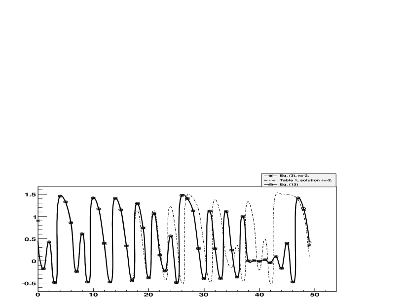
Fig. 2: Three plots of the logistic map (3) for $r=-2$ and the same initial condition $x_{0}=0.9$. With stars we plot the numerical iterations of the map; the line-dot curve corresponds to the values calculated with the solutions in the form given in Table 1 and the continuous curve shows the values from solution (13), which behaves just like the iterative points.

(b) $x_{n+1}-x_{n}=rx_{n}(1-x_{n+1})$
Contrary to the previous logistic map, this one has the exact solution (5). Even more, it is possible to develop the general Riccati solution for this difference equation, as has been done before for the three site master equation [6]. By defining $x_{n,1}$ as given by solution (5), the general Riccati solution turns out to be

$$x_{n,g}=x_{n,1}+\frac{\prod_{k=0}^{n-1}g_{k}^{-1}}{\gamma+\sum_{k=0}^{n-1}\left(\prod_{j=0}^{k}g_{j}^{-1}\right)h_{k}}$$ (14)

where

$$g_{n}=\frac{r\,x_{n,1}+1}{r(1-x_{n+1,1})+1}\ \ \ \ \mbox{and}\ \ \ \ h_{n}=\frac{r}{r(1-x_{n+1,1})+1}~{}.$$

Even when this solution is difficult to interpret as the different-initial-condition form of the difference equation (4), it behaves just like in the continuum case, as can be seen in Fig. (3), where different values of the parameter $\gamma$ lead to different initial conditions.

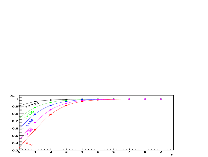
Fig. 3: The general Riccati solution for the map (4) with $x_{0}=0.333$ and $r=1.73$ for different values of the parameter $\gamma$. These solutions behave exactly as the solutions of the logistic equation (the continuous case).

Conclusion. - In this short note we have dealt with exact solutions of the logistic equation and logistic maps. After presenting the general Riccati solution for the logistic equation, we introduce a simpler form of the solution of the standard logistic map (3) which is more accurate than the solution cited in the literature. We also show that the slightly modified logistic map (4) is the closest difference representation of the logistic equation from the point of view of its general Riccati solution. Moreover, in the latter case, the general solution (14) that we provide here is valid for any value of the parameter $r$ whereas in the first case the analytic solution is restricted to only three values so far. For a different argument in favor of the form (4), the reader is directed to the recent work of Takenouchi and Ota [7].

***

We acknowledge support from CONACYT of Mexico, through a scholarship for M. Ranferi Gutiérrez.

References

-
[1]
May R H 1976
Simple mathematical models with very complicated dynamics
Nature 261 459 -
[2]
Morishita F 1965
The fitting of the logistic equation equation to the rate of increase of population density
Res. Population Ecol. 7 52
Hirota R 1979
Nonlinear partial difference equations. V. Nonlinear equations reducible to linear equations
J. Phys. Soc. Japan 46 312 -
[3]
Elaydi S N 2000
Discrete Chaos (Boca Raton: Chapman and Hall/CRC) -
[4]
Wolfram S 2002
A New Kind of Science (Champaign: Wolfram Media) p 918 -
[5]
Ulam S M and Von Neumann J 1947
On combination of stochastic and deterministic processes
Bull. Math. Soc. 53 1120 -
[6]
Rosu H C, Reyes M A and Valencia F 2005
Three-step master equation: parametric stationary solution
Int. J. Theor. Phys. 44 1565 -
[7]
Takenouchi Y and Ota Y 2009
Effect of the time delay on the stability and instability of the logistic map
arXiv:0908.3970