Synchronization of spatio-temporal chaos as an absorbing phase transition: a study in $2+1$ dimensions

Abstract

The synchronization transition between two coupled replicas of spatio-temporal chaotic systems in 2+1 dimensions is studied as a phase transition into an absorbing state — the synchronized state. Confirming the scenario drawn in 1+1 dimensional systems, the transition is found to belong to two different universality classes — Multiplicative Noise (MN) and Directed Percolation (DP) — depending on the linear or nonlinear character of damage spreading occurring in the coupled systems. By comparing coupled map lattice with two different stochastic models, accurate numerical estimates for MN in $2+1$ dimensions are obtained. Finally, aiming to pave the way for future experimental studies, slightly non-identical replicas have been considered. It is shown that the presence of small differences between the dynamics of the two replicas acts as an external field in the context of absorbing phase transitions, and can be characterized in terms of a suitable critical exponent.

Keywords: Phase-transitions into absorbing states (Theory), percolation problems (Theory), non-equilibrium wetting (Theory).

1 Introduction

Synchronization of low dimensional chaotic oscillators, which have been intensively investigated in the last two decades [1], can be essentially regarded as a bifurcation from an uncorrelated to an entrained state. When single low dimensional oscillators are replaced by spatially extended systems exhibiting spatio-temporal chaos, however, synchronization becomes a genuine, fluctuation driven, phase transition which separates the uncorrelated and the completely synchronized states [2, 3]. The synchronization transition (ST) between two identical coupled replicas (starting from different, generic initial conditions) of the same spatio-temporal chaotic dynamics is thus a non-equilibrium critical phenomenon originating from deterministic dynamics. Chaotic fluctuations on the synchronized trajectory play the role of intrinsic stochastic terms, leading to diverging fluctuations as the critical point is approached [4].

Numerical studies in one dimensional dissipative extended systems have shown that the ST is essentially a phase transition into an absorbing state [5], i.e. the completely synchronized state, in which the two replicas of the extended system evolve on the same chaotic trajectory [2, 3], similarly to low dimensional chaotic systems [6]. Noticeably, the observed continuous STs can be distinguished in two universality classes depending on the spatio-temporal propagation properties of the system close to criticality [2]. Consider a localized and finite perturbation (or synchronization error) to one of two otherwise identical (and thus synchronized) coupled replicas. At low coupling it will spread with a well defined propagation velocity $v_{F}$ [7], implying a desynchronization of the two replicas. By definition, ST takes place at the critical coupling value for which $v_{F}$ vanishes, i.e. the synchronization error does not propagate anymore in space and time. On the other hand, the evolution of “infinitesimal” synchronization errors is well described by the linearized dynamics and can be characterized in terms of the asymptotic exponential growth rate, i.e. the so-called transverse Lyapunov exponent $\lambda_{T}$ [1, 6]: a positive (resp. negative) $\lambda_{T}$ implies exponential growth (resp. contraction) of infinitesimal perturbations. Whenever the local dynamics is sufficiently smooth, i.e. the linearization captures the essential features of the full dynamics, $\lambda_{T}$ vanishes together with $v_{F}$ at the critical coupling for the synchronization. When this happens ST belongs to the Multiplicative Noise (MN) universality class [9]. When strong nonlinear effects make finite amplitude perturbations more unstable than infinitesimal ones [10], the transverse Lyapunov exponent vanishes before the error propagation velocity, so that at the ST transition one has $\lambda_{T}<0$ and $v_{F}=0$. In this second case, which is closely related to the Stable Chaos phenomenon [11], ST belongs to the Directed Percolation (DP) universality class [5]. In the framework of one dimensional coupled map lattices (CMLs) – a common prototype of spatio-temporal chaotic systems – the critical behavior belongs to the DP universality class for (almost-)discontinuous local maps, and to the MN class for smoother maps [2, 3]. Remarkably, in the context of CMLs models, it is possible to pass from DP to MN by varying a unique parameter, which controls the strength of nonlinear instabilities of the local map [12].

Analytical arguments (coarse-graining techniques combined with linearization or finite-size analysis) show that these two STs can be mapped into the Langevin equations describing the MN or DP universality classes, respectively [3, 7]. It is worth noticing that these two universality classes have been originally identified in completely different contexts, such as epidemics spreading in reaction diffusion dynamics (DP) or the depinning of a fluctuating Kardar-Parisi-Zhang (KPZ) [13] interface (with a negative nonlinear term) from an underlying substrate (MN). Interestingly, while it is not possible to define a simple reaction diffusion system with a Markov dynamics belonging to the MN class, DP critical depinning can be observed when a short ranged attraction force is imposed between a KPZ interface and the underlying substrate [14]. Therefore, ST can be described in terms of a single Langevin equation [15]. Although it is yet unclear how the empirical Langevin equation for ST may eventually flow – as a control parameter is varied from the MN to the DP region – to the same DP fixed point as the Langevin equation for Reggeon field theory, these results strongly suggest that both universality classes may be described within a unique field-theoretic framework.

In the last few years, ST has been object of intensive numerical investigations [2, 3, 7, 12, 17, 16, 18, 19]; the analysis has also been extended to stochastic coupling [2], cellular automata [20, 21], systems with long-range interactions [22, 23] and delayed dynamical systems [24, 25], exploiting the analogy between the latter and spatially extended dynamics. So far, however, ST critical behavior has been investigated in 1+1 dimensions only. In this respect, it should be also remarked that while DP critical exponents are known with great accuracy in any dimension, and MN exponents have been accurately measured in 1+1 dimensions [26], the only known estimates of the MN critical indexes in 2+1 dimensions comes from direct numerical simulations of the Langevin dynamics [27]. Moreover, it is worth recalling that, for $d\leq 2$ the MN critical behavior is completely governed by a strong coupling fixed point [28], so that no field theoretical estimates of critical exponents are currently available.

The above situation is particularly unsatisfactory, especially considering that two dimensional spatio-temporal chaotic systems – such as chemical turbulence in quasi-two dimensional reactions [29, 30] or turbulent nematic liquid crystals [31] – are the most promising ones for studying ST in experiments. In this perspective, it is worth stressing that no experimental realization of the MN class has been so far realized, and it is only recently that the DP critical exponents have been measured in experiments: in 1+1 [32] and 2+1 dimensions [31]. Therefore, besides the potential interest of experimentally realizing synchronization of chaotic extended systems, such an experiment would be the perfect ground for testing MN critical behavior in a physical framework.

A major difficulty in devising a synchronization experiment is the assemblage of two perfectly identical replicas of the same system. In practice, it would be unavoidable to experience very small differences, e.g., in the physical parameters entering the dynamics of the two systems. It is therefore of practical interest to quantify the influence of a small mismatch in the copies of the two systems. Another difficulty could lie in producing a suitable local coupling between the two replicas. However, this can be also realized through a stochastic forcing, for instance exposing two excitable chemical samples to the same random illumination (see, e.g., [30]), or by applying the same random external voltage to two replicas of the intermittent electrohydrodynamic convection regimes of Ref.[31]. As far as the critical properties of ST are concerned, deterministic or stochastic couplings are expected to share the same properties [2, 3].

This paper focuses on the synchronization transition in two spatial dimensions, within the framework of CMLs, with a twofold scope. First, we aim at verifying whether the scenario drawn in one dimensional systems for ST applies also to two dimensions. This requires accurate estimates of the MN critical exponents. For such reason we also investigate two stochastic models which are expected to belong to MN universality class. Second, mimicking what could happen in an experiment, we study ST in the presence of a small parameter mismatch between the two replicas.

The paper is organized as follows. In Sect. 2, after presenting the CMLs models and recalling the definition and basic tools for measuring the critical exponents, we discuss the results of accurate numerical simulations for two different classes of maps, which in 1+1 dimensions have been proved to belong to the DP and MN universality classes. Sect. 3 focuses on accurate estimation of critical exponents for MN class in $2+1$ dimensions by means of two stochastic models. The section ends with a critical comparison between the computed exponents for the MN universality class and some scaling relations which have been put forward by previous studies. In Sect.4, mimicking what would typically be an experimental setting, we reconsider ST in the presence of a parameter mismatch and, accordingly, we introduce a new critical exponent for its characterization. Sect. 5 is devoted to final remarks and discussions.

2 Synchronization transition in two spatial dimensions

In the following we investigate the dynamics of two coupled replicas of two dimensional CMLs, defined on a $L\times L$ square lattice with periodic boundary conditions, evolving according to the dynamics:

$$u_{t+1}(x,y) = (1-\gamma)F(\tilde{u}_{t}(x,y))+\gamma F(\tilde{v}_{t}(x,y))$$

$$v_{t+1}(x,y) = (1-\gamma)F(\tilde{v}_{t}(x,y))+\gamma F(\tilde{u}_{t}(x,y))$$ (1)

with $x,y=1,2,\ldots,L$. The variable

$$\tilde{z}_{t}(x,y) = \nabla^{2}_{\varepsilon}z_{t}(x,y)\equiv(1-\varepsilon)z_{t}(x,y)$$

$$+ \frac{\varepsilon}{4}[z_{t}(x+1,y)+z_{t}(x-1,y)+z_{t}(x,y+1)+z_{t}(x,y-1)]\,,$$

(with ${z}={u},{v}$) represents the nearest-neighbour diffusive coupling within each replica. Through this work, we set the diffusive coupling constant $\varepsilon$ equal to the democratic value $\varepsilon=4/5$, that gives same weight to all neighbors. As from studies in the one dimensional version of Eq. (1), the DP or MN character of the ST relates to the functional form of the local map $F(u)$ [2, 3]. In particular, we have that if $F(u)$ is continuous (such as the logistic or the tent map) the transition is in the MN universality class. Conversely, for discontinuous (or quasi-discontinuous [34]) maps, such as the generalized shift map

$$F(u)=au\quad\mathrm{mod}\;1\,,$$ (3)

the ST belongs to the DP-class. The strength of the “transverse” coupling between the replicas is controlled by $\gamma$: for $\gamma=0$ they are completely uncorrelated, while setting $\gamma=1/2$ induces trivial complete synchronization in one time step, i.e. $u_{t}(x,y)=v_{t}(x,y)$ for any $t\geq 1$ and for all $x,y$. Nontrivial ST, if present, is expected for a critical coupling value $\gamma_{c}\in\,]0:1/2[$ at which the synchronized state, $u_{t}(x,y)=v_{t}(x,y)$, becomes stable (or, at least, marginally stable). For any $\gamma\geq\gamma_{c}$, the two replicas (starting from different, generic initial conditions) converge toward the same spatio-temporal chaotic trajectory. In other terms, the synchronization error field $w_{t}(x,y)=|u_{t}(x,y)-v_{t}(x,y)|$ tends towards zero for any $x,y$. The linear stability properties of the synchronized state are ruled by the transverse Lyapunov exponent $\lambda_{T}$. For $\gamma\geq\gamma_{c}$, $\lambda_{T}$ can be directly computed from the maximum Lyapunov exponent $\lambda$ of an uncoupled replica according to the relation [6]

$$\lambda_{T}=\lambda+\ln(1-2\gamma)\,.$$ (4)

The request $\lambda_{T}=0$ thus determines the coupling $\bar{\gamma}=(1-\exp(-\lambda))/2$, which coincides with the critical coupling for ST, i.e. $\bar{\gamma}=\gamma_{c}$, for maps belonging to the MN class. However, this result, based on the linear analysis, does not hold for systems belonging to the DP universality class.

The suitable order parameter to characterize ST is the spatial average of the synchronization error $w_{t}(x,y)=|u_{t}(x,y)-v_{t}(x,y)|$, i.e.

$$\rho(t)=\frac{1}{L^{2}}\sum_{x,y=1}^{L}w_{t}(x,y)\,.$$ (5)

Note that $\rho(t)=0$ if and only if $w_{t}(x,y)=0$ for all $x,y$. If two replicas are identical (i.e. synchronized) at time $t_{0}$, they will remain so at all times $t\geq t_{0}$, implying that the synchronized state is absorbing, i.e. the dynamics cannot escape from it.

Interestingly, the MN and DP absorbing states differ in their measure [33] which, for any finite system size $L$, is vanishing or finite, respectively. As a consequence any finite system belonging to the DP class falls into the absorbing state in a finite time. In CMLs, whose state variables are continuous, the synchronized state $w_{t}(x,y)=0$ can only be reached asymptotically in time (barring computer round-offs), apparently at odd with the nature of the DP absorbing state. In Ref. [7], however, it has been shown that whenever the ST transition takes place at $v_{F}=0$ and $\lambda_{T}<0$ (the DP case), all perturbations smaller than a certain finite (but vanishing for $L\to 0$) threshold are exponentially contracted towards zero, thus defining an effective finite measure for the absorbing state.

We now consider the scaling theory for phase transitions into an absorbing state [5], which allows for defining the universal critical exponents, only depending on properties such as system symmetries and spatial dimensions, in terms of which we can characterize the ST. In the thermodynamic limit and at $\gamma=\gamma_{c}$, one expects the order parameter to follow the asymptotic power law decay

$$\rho(t)\sim t^{-\theta}\,,$$ (6)

where $\theta$ is a critical exponent. Close to the critical point, but slightly within the unsynchronized phase, i.e. for $\gamma<\gamma_{c}$ and $\gamma_{c}-\gamma\ll 1$, the asymptotic value of the order parameter $\rho_{\infty}\equiv\lim_{T\to\infty}\frac{1}{T}\sum_{t=1}^{T}\rho(t)$ is characterized by the scaling relation

$$\rho_{\infty}\sim(\gamma_{c}-\gamma)^{\beta}\,,$$ (7)

which defines a second critical exponent. Out of equilibrium critical phenomena are also characterized by the divergence of space and time correlations close to the critical point, in particular one expects

$$\xi_{\parallel}\sim|\gamma-\gamma_{c}|^{\nu_{\parallel}}\,,\qquad\quad\xi_{\perp}\sim|\gamma-\gamma_{c}|^{\nu_{\perp}}$$ (8)

where $\xi_{\parallel}$ (resp. $\xi_{\perp}$) is the temporal (resp. spatial) correlation length, where for simplicity we considered the system to be spatially isotropic. It can be shown [5] that only three exponents are independent, and in particular that the following relation holds

$$\theta=\beta\nu_{\parallel}\,.$$ (9)

Furthermore, the ratio $z=\nu_{\parallel}/\nu_{\perp}$, i.e. the so-called dynamical exponent, determines the relation between time and space correlations. The dynamical exponent can be measured exploiting the finite-size scaling relation

$$\rho(t)=L^{-\theta z}f(t/L^{z})\,,$$ (10)

which holds at the critical point ($f$ being a universal scaling function).

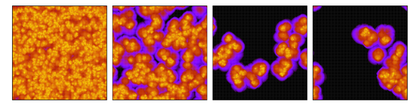
Figure 1: Snapshots of the synchronization error field $w_{t}(x,y)$ at four successive times (increasing from left to right) for a $2d$-lattice of $256\times 256$ coupled Bernoulli shift maps. The two replicas are transversely coupled with $\gamma=0.32824$, slightly above the critical point. Color code goes from light toward black indicating decreasing intensity of the field (in logarithmic scale).

2.1 Discontinuous Maps and Directed Percolation universality class

We start analyzing the synchronization transition of two different replicas of the same CML (1) whose local dynamics is given by a discontinuous map. In particular, we consider the Bernoulli map (3) with $a=2$. Fig. 1 displays the typical spatial structure of the difference field $w_{t}(x,y)$, as obtained iterating two replicas starting from (independent) random initial conditions, at successive times, for $\gamma$ slightly larger than the critical coupling value. The figure reveals typical DP patterns in proximity of the synchronization threshold. In order to make quantitative such observation, we need to measure the critical exponents. To this aim, we preliminarily determined the critical point by a careful finite-size analysis of the order parameter time decay. In particular, considering systems’ sizes up to $L=4096$, we obtained $\gamma_{c}=0.32817(2)$. Being the maximum Lyapunov exponent of the single CML $\lambda=\ln 2$, from Eq. (4) one can derive $\lambda(\gamma_{c})=-0.3749$. Thus the ST takes place at a definitely negative Lyapunov exponent and the synchronized state is truly absorbing [7].

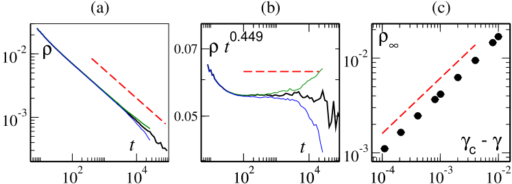
Figure 2: Critical behaviors of ST for CMLs of Bernoulli maps, data refer to a $1024\times 1024$ lattice. (a) Order parameter as a function of time at criticality $\gamma_{c}=0.32817$ (black line) and slightly below ($\gamma=0.32815$) and above ($\gamma=0.32819$) the critical point (coloured thin lines). Data are averaged over $200$ initial conditions. The dashed red line marks the $t^{-\theta}$ behavior with $\theta=0.449$. (b) The compensated order parameter $\rho(t)t^{\theta}$ reveals a satisfactory plateau over about two decades. (c) Asymptotic order parameter $\rho_{\infty}$ as a function of the distance from the critical point. The dashed red line shows the best fit with $\beta=0.584(9)$. For each $\gamma$, $\rho_{\infty}$ is obtained averaging over $100$ initial conditions.

We evaluate the exponent $\theta$ at criticality by averaging the instantaneous order parameter over about $200$ independent initial conditions in systems of size $L=1024$, obtaining a convincing straight line in a doubly logarithmic plot (Fig. 2a). The best fit provides $\theta=0.449(4)$, which is perfectly compatible with the best DP numerical estimates in $2+1$ dimensions, that is $\theta_{DP}=0.451(6)$ [5]. The quality of such a scaling law is tested by multiplying the order parameter $\rho(t)$ by $t^{\theta}$, as shown in in Fig. 2b we obtain an almost two decades long plateau.

We next compute $\rho_{\infty}$ for several $\gamma$ below the critical point at $L=1024$. By averaging over $\approx 100$ different initial conditions we estimate $\beta=0.584(9)$ (Fig. 2c), to be compared with the DP estimate $\beta_{DP}=0.584(4)$. The larger error is mainly due to the uncertainty on the location of the critical point.

Finally, we determine the dynamical exponent $z$ through the finite-size scaling relation (10). Our best data collapse (shown in Fig. 3a) suggests $z=1.77(3)$. All together, the three critical exponents $\theta$, $\beta$ and $z$ completely identify the DP universality class.

In Table 1 the results are summarized together with the exponent for DP in $d=2$ as obtained from the best known numerical estimates reported in Ref. [5]. The agreement is very good and we can safely affirm that the ST of map with discontinuities in $d=2$ is in the DP universality class, confirming the one dimensional findings.

	$\theta$	$\beta$	$z$
Bernoulli	0.449(4)	0.584(9)	1.77(3)
DP [5]	0.451(6)	0.584(4)	1.76(3)

Table 1: Critical exponents for coupled Bernoulli maps in $2+1$ dimensions together with the best estimations of the critical indexes for DP in $d=2$. For DP $\theta$ and $z$ have been derived by employing $\nu_{\parallel}=1.295(8)$ and $\nu_{\perp}=0.733(6)$ [5].

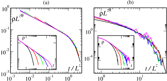
Figure 3: The finite size scaling collapse for ST in CMLs according to Eq. (10) is employed to estimate the exponent $z$. (a) Collapse for CMLs of Bernoulli maps obtained using $\theta=0.449$ and $z=1.77$. Inset: non rescaled data for $L=16,32,64,128,256$ (from left to right). (b) Collapse for skewed tent maps (see Sec. 2.2) obtained using $\theta=1.81$, $z=1.55$. Inset as in (a). Data have been averaged from $10^{2}$ up to $10^{4}$ realizations depending on the system size

2.2 Continuous Maps and Multiplicative Noise universality class

We now study the synchronization transition in CMLs with continuous local maps. In particular, we consider the system (1) with local dynamics given by the skewed tent map on the unit interval, namely

$$F(x)=\left\{\begin{array}[]{ll}ax&\mbox{if}\,\,x\leq 1/a\\ a(x-1)/(1-a)&\mbox{if}\,\,x>1/a\\ \end{array}\right.\,$$ (11)

where we set $a=2.2$. The skewed tent map is the simplest generic continuous map; the skewness ensures the fluctuation of the multipliers (first derivatives of the map) in tangent space, which is the generic behavior [6]. Similarly to Fig. 1, Fig. 4 illustrates the spatio-temporal evolution of the synchronization error field $w_{t}(x,y)$ for $\gamma$ slightly larger than the critical coupling value. Already at first glance, comparing the two figures one can argue that the two STs should belong to different universality classes. It is also apparent the different nature of the absorbing state (in black).

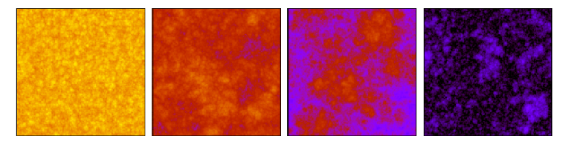
Figure 4: Same as Fig.1 for coupled skewed tent maps. The transversal coupling is $\gamma=0.132$, slightly above the critical point. The color coding and the scale are the same as Fig.1.

To make quantitative the above statement, as for the previous case, we first identified the critical coupling $\gamma_{c}$ at which ST takes place.

From the time decay of the order parameter $\rho(t)$ we estimated $\gamma_{c}=0.131760(5)$. This value appears to be compatible with the requirement that the transverse Lyapunov exponent $\lambda_{T}$ vanishes at the MN synchronization transition. Indeed, from an independent numerical simulation of a single replica, we found that the largest Lyapunov exponent is $\lambda=0.30588(6)$, which through Eq. (4) yields $\lambda_{T}=0.00001(6)$. Thus the ST now takes place at a zero transverse Lyapunov exponent. It should be mentioned that to minimize finite size effects, which are rather severe in this case (as discussed in the following) we have considered lattice up to size L=8192.

Once the critical point is known, we can estimate the critical exponents. In Fig. 5a-b we report the results on the time decay of the order parameter at criticality. The critical exponent $\theta$ is estimated by multiplying $\rho(t)$ by $t^{\theta}$ and varying $\theta$ as to maximize the size of the flat plateau. However, it is worth stressing that, at variance with the case of discontinuous maps, here finite-size effects are more severe and numerical artifacts may be present. In particular, the asymptotic power law decay sets in at later times with respect to discontinuous maps. Moreover, the critical exponent is larger than the corresponding DP value, so that lack of statistics tends to plague late time data. Therefore, it is necessary to explore large lattice sizes to obtain reasonable scaling and rule out finite-size effects. We performed numerical simulations in systems of size $L=8192$, averaging over three independent realizations, obtaining slightly more than a decade of convincing scaling behavior. We estimate $\theta=1.81(5)$.

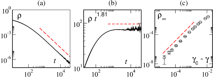
Figure 5: Critical behavior of ST for CML’s of skewed tent maps (11) with $a=2.2$. (a) Power law decay of the order parameter at $\gamma_{c}$, the dashed line marks the $t^{-\theta}$ power law with $\theta=1.81$. Data have been obtained by averaging over three realizations with system size $L=8192$ and by a further logarithmic-window average in time. (b) The order parameter is multiplied by $t^{1.81}$ to obtain an asymptotically flat curve. (c) Subcritical behavior computed from simulations at system size $L=4096$. The dashed red line marks a slope of $2.19$.

As it is shown in Fig. 5c, the behavior of the saturated order parameter $\rho_{\infty}$ in the subcritical regime ($\gamma<\gamma_{c}$), allows us to measure the second critical exponent. Our best estimates, in systems of linear size $L=4096$ give us $\beta=2.19(9)$.

For phase transitions in the MN universality class, the dynamical exponent $z$ has been conjectured (and confirmed by numerical simulations in 1+1 dimensions) to coincide with the one associated to the KPZ equation [35]. Indeed, as it will become clearer in Sect. 3, the MN synchronization problem can be mapped in the depinning transition of a bounded KPZ surface. From this mapping one deduces that at the critical point, where the interface asymptotically depins, MN systems should exhibit the same space and time correlations as free KPZ ones. Thus they are also characterized by the same $z$ exponent. By rescaling finite size data averaged over many realizations with $\theta=1.81$ by means of relation (10), we obtained $z=1.55(8)$ (see Fig. 3b), which is compatible with the known best estimates of KPZ dynamical exponent in 2+1 dimensions, $z_{KPZ}=1.607(3)$ as reported in Ref. [36].

3 Stochastic Models and Scaling Arguments

As far as we know, the only measurement of MN critical exponents in two spatial dimensions reported in literature [27] was obtained by numerically investigating the associated Langevin equation. In order to obtain independent and accurate estimations of the critical indexes, we studied two stochastic models which are known, in 1+1 dimensions, to belong to the MN universality class.

3.1 Single Step model plus a hard wall (SSW)

The MN universality class is closely related to the depinning of a KPZ surface from a hard substrate. Indeed the MN Langevin equation [9]

$$\partial_{t}\phi=b\phi-c\phi^{2}+D\nabla^{2}\phi+\phi\eta$$ (12)

can be formally mapped, via the Cole-Hopf transformation $\psi({\bf r},t)=-\ln\phi({\bf r},t)$, onto the KPZ equation with negative nonlinear term and bounded from below [15]

$$\partial_{t}\psi=v_{0}-ce^{-\psi}+D\nabla^{2}\psi-D\left(\nabla\psi\right)^{2}+\eta\,.$$ (13)

Here, $\psi({\bf r},t)\geq 0$ and $\phi({\bf r},t)\in[0,1]$ are the coarse-grained height and difference field, respectively, while $\eta({\bf r},t)$ is a spatio-temporal Gaussian white noise, and $D>0$. Note that the $\phi({\bf r},t)=0$ absorbing state of the Langevin dynamics corresponds to an infinite height (i.e. a completely depinned) interface in the bounded KPZ representation.

The above link suggests us to consider a simple solid-on-solid stochastic deposition model, belonging to the KPZ universality class, such as the well known single step model (SSM), which in one spatial dimension can be exactly mapped onto the KPZ equation (see, e.g., Ref. [37], see also Ref.[38] for a study in two spatial dimensions). Equipped with a hard substrate, the so-called SSM-plus-wall (SSW) provides an example of MN phase transition. In 1+1 dimension, the critical point is analytically known and very accurate numerical estimates of MN critical exponents have been obtained [14, 26]. The SSW time-depinning exponent $\theta$ has also been computed in one spatial dimension via a mean field-like approximation in Ref. [39].

Here, we numerically investigate the following two dimensional generalization of the SSW model. A fluctuating interface with an integer height field $h_{t}(x,y)$ is defined on a square lattice ($x,y=1,2,\ldots,L$) with periodic boundary conditions. The dynamics of the interface is subjected to the following restrictions: the heights on nearest neighbours sites cannot be equal and must differ by one, i.e. $|h_{t}(x,y)-h_{t}(x\pm 1,y)|=|h_{t}(x,y)-h_{t}(x,y\pm 1)|=1$, moreover a hard lower wall at height $H_{t}$ moving upward with velocity $V_{w}$ is imposed requiring that $h_{t}(x,y)>H_{t}$, with $H_{t}=V_{w}t$. The dynamics is asynchronous: at each sub-time step $dt=1/L^{2}$ a site $(x,y)$ is chosen at random and its height is increased by two, $h_{t+dt}(x,y)=h_{t}(x,y)+2$, if $h_{t}(x,y)$ is a local minima. Finally, the wall moves up by one unit every $L^{2}/V_{w}$ time steps pushing up the interface: every site whose height is less than $H_{t}$ is raised by two units. The density $\rho$ of interface sites attached to the interface (i.e. $h_{t}(x,y)=H_{t}$) immediately after a wall movement is the proper order parameter, while the wall velocity $V_{w}$ is the control parameter.

Unfortunately, the critical velocity $V_{w,c}$ of the two dimensional SSW is not known analytically. Careful finite-size analysis up to $L=4096$ has been used to locate the critical depinning velocity, which is estimated to be $V_{w,c}=0.34135(10)$. Numerical simulations start from a completely pinned interface: $h_{0}(x,y)=0$ for $x+y$ odd and $h_{0}(x,y)=1$ otherwise. Our results for the time decay critical exponent $\theta$, shown in Fig 6a-b, yield $\theta=1.80(5)$. By slightly increasing the wall velocity above the critical value we can estimate the magnetization exponent, corresponding to the behavior of the ST for subcritical couplings, obtaining $\beta=2.36(9)$, as shown in Fig 6c. Summarizing, $\theta$ is in fairly good agreement with the estimate for the CML with skewed tent maps, and $\beta$, while still compatible if error bars are considered, appears to be slightly larger. Finally, the dynamical exponent $z$ is estimated via the finite-size scaling relation (10) with $\theta=1.8$. A satisfactory data collapse can be obtained with $z=1.63(5)$ (not shown), which is compatible with the value obtained for the tent map.

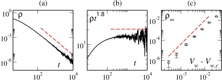
Figure 6: Critical behavior of the depinning transition in the $d=2$ SSW model with $L=4096$. (a) Power law decay of the order parameter at criticality, the dashed line marks the power law $t^{-1.8}$. Data are obtained by averaging three different realizations and by a further logarithmic-window average in time. (b) Order parameter multiplied by $t^{1.8}$ to demonstrate the quality of scaling. (c) The subcritical behavior is characterized by a power law with exponent $\beta=2.36$, as indicated by the dashed line.

It is worth concluding by remarking that in Ref. [26] it has been shown that the probability distribution of the first depinning time (i.e. the first time at which an initially flat and pinned surface depins) does not follow a standard finite scaling relations in the MN case. The numerical simulations of the SSW model, however, show that other quantities of interest, as the density of pinned sites, follow the typical scaling of absorbing phase transitions. This peculiarity can be probably ascribed to the “weakly absorbing” nature of the MN absorbing state [33].

3.2 Random Multiplier model

We now consider the Random Multiplier (RM) defined by the dynamics [7]

$$w_{t+1}(x,y)=\left\{\begin{array}[]{ll}1,&\mbox{w.p.}\quad\alpha\tilde{w}_{t}(x,y)\\ \alpha\tilde{w}_{t}(x,y),&\mbox{w.p.}\quad 1-\alpha\tilde{w}_{t}(x,y)\end{array}\right.\;\;{\rm if}\;\tilde{w}_{t}(x,y)>\Delta$$ (14)

$$w_{t+1}(x,y)=\left\{\begin{array}[]{ll}\tilde{w}_{t}(x,y)/\Delta,&\mbox{w.p.}\quad\alpha\Delta\\ \alpha\tilde{w}_{t}(x,y),&\mbox{w.p.}\quad 1-\alpha\Delta\end{array}\right.\qquad\,{\rm if}\;\tilde{w}_{t}(x,y)\leq\Delta$$ (15)

where “w.p.” is the shorthand notation for “with probability”, $w_{t}(x,y)\in[0:1]$ and $\tilde{w}_{t}(x,y)=\nabla^{2}_{\varepsilon}w_{t}(x,y)$ is the discrete diffusive operator, as in Eq. (1), with $\varepsilon=4/5$, on a square lattice ($x,y=1,2,\ldots,L$) with periodic boundary condition.

Before discussing the results of the model, it is worth briefly reviewing its properties and its meaning. The model (14)-(15) was originally introduced in Ref. [7] to describe the synchronization error evolution in proximity of the synchronization transition of both continuous and discontinuous maps. Essentially the value of parameter $\Delta$ discriminates between discontinuous or continuous character of the local dynamics, switching the behavior from the DP to the MN universality class. To better understand the origin of the model, first consider Eq. (1) equipped with the Bernoulli map (3). One can formally compute the linearized evolution equation for the synchronization error, which reads

$$w_{t+1}(x,y)=\tilde{w}_{t}(x,y)(1-2\gamma)\partial_{u}F(\tilde{u}_{t}(x,y))\,.$$ (16)

Such an equation holds locally for any finite synchronization error $w_{t}(x,y)$ such that $\tilde{u}_{t}(x,y)$ and $\tilde{v}_{t}(x,y)$ fall on the same branch of the Bernoulli map. In this case one simply has $w_{t+1}(x,y)=\tilde{w}_{t}(x,y)\,a\,(1-2\gamma)$. However, whenever $\tilde{u}_{t}(x,y)$ and $\tilde{v}_{t}(x,y)$ fall on the two different branches of the Bernoulli map, the synchronization error is typically expanded to order $1$ values, a fact overlooked by the linearization. This latter situation can occur with a probability proportional to $\tilde{w}_{t}(x,y)$ [7]. Setting $\Delta=0$, so that only Eq. (14) is relevant, reproduces the Bernoulli map dynamics with $\alpha=a(1-2\gamma)$.

On the other hand, for the skewed tent map (11) — as well as any continuous map — the full dynamics is well captured by linearized dynamics. For the local map (11) the local multiplier assumes one of the two values $\partial_{u}F(a,u)=a$ or $\partial_{u}F(a,u)=a/(1-a)$ according to the chaotic dynamics. By approximating the chaotic signal with randomly chosen multipliers, the RM model with finite $\Delta$ mimics exactly this latter situations, cfr. Eq. (15); while Eq. (14) simply provides a nonlinear saturation effect. Interestingly, in Ref. [7] it has been shown that there exist a threshold $\bar{\Delta}>0$ below which the transition still belongs to the DP class. This corresponds to the case of almost-discontinuous piecewise linear maps on the unit interval, characterized by a very steep branch (with slope $1/\Delta$ and width of order $\Delta$); for a complete discussion see Ref. [7] and [12].

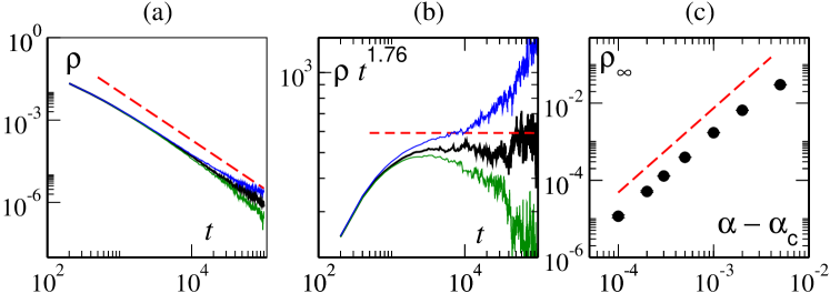
Figure 7: Critical behavior of the RM model in 2+1 dimensions with size $L=2000$. (a) Power law decay of the order parameter at criticality. Data have been obtained by averaging over $100$ realizations. The dashed line marks the power law $t^{-1.76}$. (b) Order parameter multiplied by $t^{1.76}$; notice the asymptotic plateau at large times. (c) Subcritical behavior computed from up to $400$ independent realizations, from which $\beta$ is estimated to be $2.18$ (dashed line).

In the following, being interested to the MN transition, we investigate the RM model for $\Delta=0.2$, which is a sufficiently large parameter value to drive the system into its “linear” regime. The parameter $\alpha$ is the control parameter of the transition; indeed, from Eq. (16) it follows that $\alpha$ is essentially equivalent to $(1-2\gamma)\partial_{u}F(a,u)$ so that to increase the coupling $\gamma$ in the deterministic model amounts to decrease $\alpha$ in the stochastic one. The synchronized regime is thus obtained for $\alpha$ smaller than the critical value $\alpha_{c}$.

The critical coupling $\alpha_{c}$ implies a zero transverse Lyapunov exponent; it can be estimated evaluating the value of $\alpha$ for which $\langle\ln w_{t}\rangle$ grows at most logarithmically in the linear regime [7]. This estimation is in agreement with the usual analysis performed to evaluate the critical point from the scaling of the order parameter in time (Fig. 7a). In particular, by considering lattices of linear sizes $L=2\times 10^{3}$ and $L=4\times 10^{3}$ the best scaling of $\rho(t)$ is observed at $\alpha_{c}=0.529825(5)$, in agreement with the Lyapunov estimate which gives $\alpha_{c}=0.52981(1)$. Moreover, the critical exponent is found to be $\theta=1.76(5)$, as shown in Fig. 7a-b. For $\alpha$ slightly above $\alpha_{c}$, from the saturated value of the asymptotic density we also find $\beta=2.18(8)$ (see Fig. 7c). Finally, finite size scaling via Eq. (10) gives $z=1.7(1)$ (not shown).

3.3 Scaling arguments and comparison among the critical exponents

This subsection is devoted to a discussion of the results obtained so far for the MN universality class. Our three independent estimates of the critical exponents for the MN class in 2+1 dimensions are reported in Table 2 For $\theta$ and $\beta$, ST in CMLs, the SSW and RM model are in remarkable agreement, the exponents are essentially coincident within error bars. In particular, $\theta$ also coincides with the early estimates of Ref. [27], while a remarkable difference (by a factor two) is observed for $\beta$. This is most likely due to the preliminary nature of the $d=2$ Langevin dynamics simulations [40]. It should be noted that typically a fairly small lack of accuracy in the estimation of the critical point can result in a quite large error in evaluating the exponent $\beta$. Also the dynamical exponent $z$ measured from finite size scaling essentially agrees with the expected KPZ value, see Table 2.

	$\theta$	$\beta$	z	$\nu_{\parallel}$
CML (skewed tent maps)	1.81(5)	2.19(9)	1.55(8)	1.21(8)
RM	1.76(5)	2.18(8)	1.63(5)	1.25(8)
SSW	1.80(4)	2.36(9)	1.7(1)	1.31(4)
KPZ [36] and scaling relation [35]			1.607(3)	1.32(1)

Table 2: Critical exponents for CMLs of skewed tent maps, random multipliers model (RM) and single step model with a wall (SSW). Also the values that can be deduced from scaling arguments and the KPZ numerical estimates are reported.

Exploiting the relation with free (without walls) KPZ scaling, it has also been conjectured that [35]

$$\nu_{\perp}=\frac{1}{2(z-1)}$$ (17)

which, from $z_{KPZ}=1.607(3)$ as obtained in Ref. [36], implies $\nu_{\perp}=0.824(5)$ and $\nu_{\parallel}=z\nu_{\perp}=1.32(1)$. This latter exponent can be compared with the ratio $\nu_{\parallel}=\beta/\theta$ as obtained for the models here analyzed: as reported in Table 2, there is an agreement within error bars with the KPZ estimate, as far as the RM and SSW are concerned. On the other hand, $\nu_{\parallel}$ is slightly underestimated when CMLs of skewed tent maps are considered. Altogether, KPZ estimates and the derived (via Eq. (17) temporal correlation exponent, well agree with our results in $2+1$ dimensions for both the dynamical exponent $z$ and the ratio $\beta/\theta$.

4 Synchronization in the presence of mismatch

As discussed in the introduction, in typical experimental settings it is impossible to produce two exact replicas of the same system. Systematic errors, slight differences in the preparation of the system, or inhomogeneous external influence should always be taken into account. Such small differences can be mimicked at the level of the CMLs model as a quenched random mismatch between the dynamical parameters of two otherwise identical systems (this idea was introduced in Ref. [6] in the context of low dimensional maps). In practice, we consider the following model, written in generic spatial dimension $d$:

$$u^{(1)}_{t+1}(\bm{r}) = (1-\gamma)F(a_{1}({\bm{r}}),\tilde{u}^{(1)}_{t}(\bm{r}))+\gamma F(a_{2}({\bm{r}}),\tilde{u}^{(2)}_{t}(\bm{r}))$$

$$u^{(2)}_{t+1}(\bm{r}) = (1-\gamma)F(a_{2}({\bm{r}}),\tilde{u}^{(2)}_{t}(\bm{r}))+\gamma F(a_{1}({\bm{r}}),\tilde{u}^{(1)}_{t}(\bm{r}))$$ (18)

where ${\bm{r}}$ is a $d$ dimensional vector and

$$\tilde{u}^{(i)}(\bm{r})=(1-\varepsilon)u^{(i)}(\bm{r})+\frac{\varepsilon}{2d}\sum_{\bm{r}^{\prime}\in NN\{\bm{r}\}}u^{(i)}(\bm{r}^{\prime})\,,$$ (19)

where the sum runs over the nearest neighbours of ${\bm{r}}$, denoted as $NN\{\bm{r}\}$. The local map $F(a,u)$ depends both on the dynamical variable $u\equiv\tilde{u}^{(i)}_{t}({\bm{r}})$ and on the quenched parameter $a\equiv a_{i}({\bm{r}}$) (where $i=1,2$ labels the replica). Periodic boundary conditions are considered as usual in a $d$-cube of linear dimension $L$. We consider two cases, the skewed tent map defined in Eq. (11) and the Bernoulli one (Eq. (3)). Without loss of generality, we can write the map parameter $a$ as

$$a_{i}({\bm{r}})=a_{0}+\omega_{i}({\bm{r}}),$$ (20)

with $\omega_{i}({\bm{r}})$ being a quenched random variable uniformly distributed in $[-h,h]$.

Let us now consider the linearized dynamics for the synchronization error $w_{t}(\bm{r})=u^{(1)}_{t}(\bm{r})-u^{(2)}_{t}(\bm{r})$, which reads as (see also [6])

$$w_{t+1}(\bm{r})=\tilde{w}_{t}(\bm{r})(1-2\gamma)\partial_{u}F(a_{1}({\bm{r}}),\tilde{u}^{(1)}_{t}(\bm{r}))+(1-2\gamma)\delta a(\bm{r})\partial_{a}F(a_{1}({\bm{r}}),\tilde{u}^{(1)}_{t}(\bm{r}))\,,$$ (21)

where $\delta a(\bm{r})\equiv a_{1}(\bm{r})-a_{2}(\bm{r})$ is the parameter mismatch. Obviously, $||\delta a(\bm{r})||\sim h$ (regardless of the chosen norm). The first term on the r.h.s. of Eq. (21) — i.e. the fluctuating “field derivative” $(1-2\gamma)\partial_{u}F(a,u)$ — leads as usual to a stochastic term proportional to the amplitude of the synchronization error itself. While the second term — i.e. the “parameter derivative” $(1-2\gamma)\partial_{a}F(a,u)$ —, also typically fluctuates according to local dynamics, but it depends only on the parameter mismatch amplitude and thus acts as an effective “external field” which locally prevent the complete synchronization of two replicas. At a field theoretical level, this suggests to describe the parameter mismatch as an external driving field with amplitude $h$. For instance, considering the MN class, one can add an additive Gaussian white noise $\zeta$ to the Langevin equation (12)

$$\partial_{t}\phi=b\phi-c\phi^{2}+D\nabla^{2}\phi+\phi\eta+h\zeta\,.$$ (22)

Implicit in the above formulation is the assumption that the noise terms $\eta$ and $\zeta$ are completely decorrelated. Of course, the statistical independence between the second and the first term in the r.h.s. of Eq. (21) has to be tested a posteriori. Unfortunately, we are not able to solve analytically Eq. (22). While efficient numerical methods [41] are known to directly simulate multiplicative noise Langevin equations, we choose instead to focus on microscopic models. We consider the RM model (23-24). The external field then can be described as an extra additive white noise $\chi(\bm{r})$ uniformly distributed in $[0,h]$, so that

$$w_{t+1}({\bm{r}})=\left\{\begin{array}[]{ll}1+\chi_{t}({\bm{r}}),&\mbox{w.p.}\quad\alpha\tilde{w}_{t}({\bm{r}})\\ \alpha\tilde{w}_{t}({\bm{r}})+\chi_{t}({\bm{r}}),&\mbox{w.p.}\quad 1-\alpha\tilde{w}_{t}({\bm{r}})\end{array}\right.\;\;{\rm if}\;\tilde{w}_{t}({\bm{r}})>\Delta$$ (23)

$$w_{t+1}({\bm{r}})=\left\{\begin{array}[]{ll}\tilde{w}_{t}({\bm{r}})/\Delta+\chi_{t}({\bm{r}}),&\mbox{w.p.}\quad\alpha\Delta\\ \alpha\tilde{w}_{t}({\bm{r}})+\chi_{t}({\bm{r}}),&\mbox{w.p.}\quad 1-\alpha\Delta\end{array}\right.\qquad\,{\rm if}\;\tilde{w}_{t}({\bm{r}})\leq\Delta$$ (24)

Indeed, the additive noise term $\chi({\bm{r}})$ creates local activity with an amplitude proportional to $h$, thus preventing complete synchronization between the two replicas.
In the following we compare direct numerical simulations of the modified RM model (23-24) with the ones of the coupled CMLs (18) with skewed tent maps with a quenched mismatch. We expect the asymptotic order parameter $\rho_{\infty}$ to saturate to an $h$-dependent value, that at criticality should scale as

$$\rho_{\infty}\sim h^{\kappa}$$ (25)

where $\kappa$ is a new critical index (associated to the external field in the field theoretical treatment).

Choosing $\langle a_{i}({\bm{r}})\rangle=a_{0}=2.2$, the critical point estimated in Sec. 2 ($\gamma_{c}=0.13176$) remains unchanged for $h>0$. Equally, we set $\Delta=0.2$ for the RM model so that $\alpha_{c}=0.52981$.

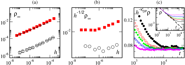
Figure 8: Critical dependence on the mismatch in CMLs in 2+1 dimensions. (a) Mismatch amplitude dependence of the saturated order parameter at criticality for skewed maps CMLs (black circles) and RM with an additive noise (red squares). The dashed red line marks the $h^{1/2}$ power law. (b) Same data as (a) rescaled by a factor $h^{-1/2}$ to highlight critical behavior. System size is $L=2048$. (c) For Bernoulli maps we check the DP expectation $\kappa_{DP}=\beta/\sigma$ by plotting $\rho(t)h^{-\kappa_{DP}}$ (see text): notice the collapse on a single plateau at large times. From top to bottom $h=10^{-7}$, $2.5\times 10^{-7}$, $6.25\times 10^{-7}$, $10^{-6}$, $2\times 10^{-6}$. System sizes is $L=1024$ and data have been averaged over $50$ initial conditions. Inset: non rescaled data compared with the $h=0$ behavior (dashed black line).

Starting from random initial conditions, we measure $\rho_{\infty}$ as a function of $h$ in both one and two spatial dimensions. The results in two spatial dimensions, reported in Fig. 8a-b, show a remarkable agreement between CMLs and the modified RM model, thus confirming that the correlations between the additive and the multiplicative terms in Eq. (21) are irrelevant. In particular, we found $\kappa=0.50(5)$ for the RM and $\kappa=0.46(7)$ for the CMLs. In one spatial dimension (not shown) we have $\kappa=0.21(2)$ (RM) and $\kappa=0.23(2)$ (CMLs). This is in rough agreement with the $d=1$ early estimates obtained by direct simulation of the Langevin equation (22) in Ref. [35]. In Ref. [28] a zero dimensional version of Eq. (22) has been exactly solved via a Fokker-Planck approach to yield a logarithmic increase with the field $h$. While we have not been able to put forward any analytical argument in $d>0$, these results lead us to conjecture $\kappa=d/4$ for MN in an external field.

We finally consider the case of Bernoulli map with $\langle a_{i}({\bm{r}})\rangle=a_{0}=2$. Here, we can exploit the fact that the scaling theory for Directed Percolation in an external field is well known (see [5] and references therein), and thus test if the dependence of $\rho_{\infty}$ on $h$ follows the DP prediction. In particular, at criticality, the order parameter should saturates to an asymptotic value $\rho_{\infty}(h)\sim h^{\kappa}$ with $\kappa=\beta/\sigma$, where $\beta$ links to the behavior of the density close to the critical point and $\sigma$ controls the mean size of inactive clusters close to the critical point, and is related to the other exponents by the formula [5]

$$\sigma=\nu_{\parallel}(d/z+1-\theta)=\nu_{\parallel}+d\nu_{\perp}-\beta\,.$$

By means of the best available DP numerical estimates [5], we have $\kappa_{DP}=0.108247(4)$ in $d=1$ and $\kappa_{DP}=0.268(4)$ in $d=2$. As shown in Fig. 8c direct numerical simulations of $2+1$ dimensional CMLs with mismatched Bernoulli maps are in very good agreement with this prediction. This is also true in $1+1$ dimensions (not shown).

5 Conclusions

The synchronization transition between spatially extended systems exhibiting spatio-temporal chaos is a prototypical example of a fluctuation driven phase transition induced by microscopic chaos. The present numerical study in 2+1 dimensions has clearly confirmed that, analogously to the 1+1 dimensional case, the synchronization transitions can been described in the framework of continuous out-of-equilibrium critical phenomena towards an absorbing phase. In particular, depending on the perturbation propagation properties of the spatio-temporal dynamics, the synchronization transition belongs to two possible universality classes, namely Directed Percolation and Multiplicative Noise. The above results confirm that the ST belongs to the DP universality class whenever the transverse Lyapunov exponent is negative at the critical point. Differently, MN behavior sets in when a zero transverse Lyapunov exponent characterize the critical point. As for the latter universality class, we have produced the best available numerical estimates of the critical exponents in two spatial dimensions. Furthermore, by analyzing different deterministic and stochastic models, we have been able to confirm universality in the MN class and its link with deposition processes.

We have also addressed the effect of a small difference in the dynamics of the two replicas, an experimentally relevant question given the practical impossibility to produce two exactly identical systems in any experimental setup. By modeling this difference as a quenched parametric mismatch in the local dynamics, we have shown that it amounts to the action of an external field within the Langevin description. Numerical simulations in one and two spatial dimensions for discontinuous local maps confirm DP scaling theory, which predicts a power law dependence of the saturated density from the external field with an exponent $\kappa$ depending from the usual zero field critical ones. Finally, we obtained an estimate for this exponent also for MN in en external field (smooth maps).

Before concluding, a comment on the behavior in higher dimensions is in order. In $d>2$ naive power counting in the MN Langevin Eq. (12) predicts the coexistence of two different fixed points in the Renormalization Group flow, a mean field one acting at small but finite noise amplitude and a strong coupling one at large noise amplitudes [28]. Estimates obtained from numerical simulations of Eq. (12) for MN in 3+1 dimensions can be found in Ref. [42].

We conclude expressing our hope that these results will stimulate experimental studies on the synchronization of extended systems exhibiting spatio-temporal chaos.

References

References

- [1] Pikovsky A S, Rosenblum M and Kurths J, Synchronization: A Universal Concept in Nonlinear Sciences, 2001 (Cambridge: Cambridge University Press)
- [2] Baroni L, Livi R, and Torcini A, in Dynamical Systems:from Cristal to Chaos, Gambaudo J M, Hubert P, Tisseur P and Vaienti S eds., 2000 (Singapore: World Scientific) p. 23; Baroni L, Livi R and Torcini A, 2001 Phys. Rev. E 63 036226
- [3] Ahlers V and Pikovsky A S, 2002 Phys. Rev. Lett.88 254101
- [4] Pikovsky A S and Kurths J, 1994 Phys. Rev. Lett.49 898; Pikovsky A S and Politi A, 1998 Nonlinearity 11 1049
- [5] Hinrichsen H, 2000 Adv. Phys. 49 815
- [6] Pikovsky A S and Grassberger P, 1991 J. Phys. A: Math. Gen.24 4587
- [7] Ginelli F, Livi R, Politi A and Torcini A, 2003 Phys. Rev. E 67 046217
- [8] Muñoz M A, de los Santos F and Achahbar A, 2003 Braz. J. Phys. 33 443.
- [9] Muñoz M A, in Advances in Condensed Matter and Statistical Mechanics, Korutcheva E, et al. eds., 2004 (New York: Nova Science Publishers)
- [10] Torcini A, Grassberger P and Politi A, 1995 J. Phys. A: Math. Gen.28 4533; Cencini M and Torcini A, 2001 Phys. Rev. E 63 056201
- [11] Politi A, Livi R, Oppo G L and Kapral R, 1993 Europhys. Lett. 22 571; Politi A and Torcini A, 2009 arXiv:0902.2545
- [12] Bagnoli F, and Rechtman R, 2006 Phys. Rev. E 73 026202
- [13] Kardar M, Parisi G, and Zhang Y C, 1986 Phys. Rev. Lett.56 889
- [14] Ginelli F, Ahlers V, Livi R, Mukamel D, Pikovsky A S, Politi A and Torcini A, 2003 Phys. Rev. E 68 065102
- [15] Muñoz M A and Pastor-Satorras R, 2003 Phys. Rev. Lett.90 204101
- [16] Bagnoli F, Baroni L, and Palmerini P, 1999 Phys. Rev. E 59 409; Bagnoli F and Cecconi F, 2001 Phys. Lett. A 282 9
- [17] Droz M and Lipowski A, 2003 Phys. Rev. E 67 056204; 2003 ibidem 68 056119
- [18] Gade P M and Hu C-K, 2006 Phys. Rev. E 73 036212
- [19] Szendro I G, Rodriguez M A, and López J M, 2009 Europhys. Lett. 86 20008
- [20] Bagnoli, F and Rechtman R, 1999 Phys. Rev. E 59 R1307
- [21] Rouquier J B, and Morvan M, 2009 J. Cell. Auto. 4 55
- [22] Tessone C J, Cencini M and Torcini A, 2006 Phys. Rev. Lett.97 224101
- [23] Cencini M, Tessone C J and Torcini A, 2008 Chaos 18 037125
- [24] Mohanty P K, 2004 Phys. Rev. E 70 045202(R)
- [25] Szendro I G and López J M, 2005 Phys. Rev. E 71 055203(R)
- [26] Kissinger T, Kotowicz A, Kurz O, Ginelli F and Hinrichsen H, 2005 JSTAT P06002
- [27] Genovese W, Muñoz M A and Sancho J M, 1998 Phys. Rev. E 57 R2495
- [28] Grinstein G, Muñoz M A and Tu Y, 1996 Phys. Rev. Lett.76 4376
- [29] Kuramoto Y, Chemical Oscillations, Waves and Turbulence, 1984 (Berlin: Springer-Verlag)
- [30] Hildebrand M, Cui J, Mihaliuk E, Wang J and Showalter K, 2003 Phys. Rev. E 68 026205
- [31] Takeuchi K A, Kuroda M, Chaté H and Sano M, 2007 Phys. Rev. Lett.99 234503; and preprint arXiv:0907.4297v1
- [32] Rupp P, Richter R, and Rehberg I, 2003 Phys. Rev. E 67 036209
- [33] Muñoz M A, 1998. Phys. Rev. E 57, 1377
- [34] Politi A and Torcini A, 1994 Europhys. Lett. 28 545
- [35] Tu Y, Grinstein G and Muñoz M A, 1997 Phys. Rev. Lett.78 274
- [36] Marinari E, Pagnani A and Parisi G, 2000 J. Phys. A: Math. Gen.33 8181
- [37] Barabási A L and Stanley H E, Fractal Concepts in Surface Growth, 1995 (Cambridge: Cambridge University Press)
- [38] Odor G, Liedke B and Heinig K-H, 2009 Phys. Rev. E 79 021125
- [39] Ginelli F, and Hinrichsen H, 2004 J. Phys. A: Math. Gen.37 11085
- [40] Muñoz M A, private communication.
- [41] Dornic I, Chaté H, and Muñoz M A, 2005 Phys. Rev. Lett.94 100601
- [42] Genovese W and Muñoz M A, 1997 Phys. Rev. E 60 69