Integrating Conflict Driven Clause Learning to Local Search

Abstract

This article introduces SatHyS (SAT HYbrid Solver), a novel hybrid approach for propositional satisfiability. It combines local search and conflict driven clause learning (CDCL) scheme. Each time the local search part reaches a local minimum, the CDCL is launched. For SAT problems it behaves like a tabu list, whereas for UNSAT ones, the CDCL part tries to focus on minimum unsatisfiable sub-formula (MUS). Experimental results show good performances on many classes of SAT instances from the last SAT competitions.

1 Introduction

The SAT problem, namely the issue of checking whether a set of Boolean clauses is satisfiable or not, is a central issue in many computer science and artificial intelligence domains, like theorem proving, planning, non-monotonic reasoning, VLSI correctness checking. These last two decades, many approaches have been proposed to solve large SAT instances, based on logically complete or incomplete algorithms. Both local-search techniques [30, 29, 19] and elaborate variants of the Davis-Putnam-Loveland-Logemann DPLL procedure [7] [28, 9], called modern SAT solvers, can now solve many families of hard SAT instances. These two kinds of approaches present complementary features and performances. Modern SAT solvers are particularly efficient on the industrial SAT category while local search performs better on random SAT instances.

Consequently, combining stochastic local search (SLS) and conflict driven clause learning (CDCL) solvers seems promising. Note that it was pointed as a challenge by Selman et al. [31] in 1997. Such methods should exploit the quality and differences of both approaches. Furthermore, the perfect hybrid method has to outperform both local search and CDCL solvers. A lot of attempts have been done last decade [5]. These different attempts will be discussed in section 3.

In this paper, we propose another hybridization of local search and modern SAT solver, named SatHyS (SAT HYbrid Solver). The local search solver is the main one. Each time it reaches a local minimum, the CDCL part is called and assigns some variables. This part of our solver is expected to have different behaviours depending on the kind of formula to solve. In case of a satisfiable one, the CDCL part can be seen as a tabu list [13] in order to protect good variables and avoid to reach the same minimum quickly. On the other hand, for unsatisfiable formulas, it tries to focus the search on minimum unsatisfiable sub-formulas (MUS) [10, 15, 16], allowing to concentrate on a small part of the whole formula. Like this, the CDCL component of SatHyS is used as a strategy to escape from local minimum.

The rest of the paper is organized as follows. Section 2 introduces different notions necessary for understanding the rest of the paper. Section 3 discusses different hybrid methods. Section 4 gives the insights of our method. In section 5, we give the details and algorithms of SatHyS. Before a conclusion, section 6 provides different experiments.

2 Preliminary definitions and technical background

2.1 Definitions

Let us give some necessary definitions and notations. Let $V=\{x_{1}...x_{n}\}$ be a set of boolean variables, a literal $\ell$ is a variable $x_{i}$ or its negation $\bar{x_{i}}$. A clause is a disjunction of literals $c_{i}=(\ell_{1}\vee\ell_{2}...\vee\ell_{n_{i}})$. A unit clause is a clause with only one literal. A formula $\Sigma$ is in conjunctive normal form (CNF) if it is a conjunction of clauses $\Sigma=(c_{1}\wedge c_{2}...\wedge c_{m})$. The set of literals appearing in $\Sigma$ is denoted $\mathcal{V}_{\Sigma}$. An interpretation $\mathcal{I}$ of a formula $\Sigma$ associates a value $\mathcal{I}(x)$ to variables in the formula. An interpretation is complete if it gives a value to each variable $x\in\mathcal{V}_{\Sigma}$, otherwise it is said partial. A clause, a CNF formula and an interpretation can be conveniently represented as sets. A model of a formula $\Sigma$, denoted $\mathcal{I}\models\Sigma$, is an interpretation $\mathcal{I}$ which satisfies the formula $\Sigma$ i.e. satisfies each clause of $\Sigma$. Then, we can define the SAT decision problem as follows: is there an assignment of values to the variables so that the CNF formula $\Sigma$ is satisfied?

Let us introduce some additional notations.

• The negation of a formula $\Gamma$ is denoted $\bar{\Gamma}$

• $\Sigma_{|_{\ell}}$ denotes the formula $\Sigma$ simplified by the assignment of the literal $\ell$ to true. This notation is extended to interpretations: Let $\mathcal{P}=\{\ell_{1},...,\ell_{n}\}$ be an interpretation, $\Sigma_{|_{\mathcal{P}}}=(...(\Sigma|_{\ell_{1}})...|_{\ell_{n}})$ ;

• $\Sigma^{*}$ denotes the formula $\Sigma$ simplified by unit propagation;

• $\models_{*}$ denotes logic deduction by unit propagation: $\Sigma\models_{*}l$ means that the literal $x$ is deducted by unit propagation from $\Sigma$ i.e. $(\Sigma\wedge\bar{\ell})^{*}=\bot$ . One notes $\Sigma\models_{*}\bot$ if the formula is unsatisfiable by unit propagation.

• $\eta[x,c_{i},c_{j}]$ denotes the resolvent between a clause $c_{i}$ containing the literal $x$ and $c_{j}$ a clause containing the opposite literal $\neg x$. In other words $\eta[x,c_{i},c_{j}]=c_{i}\cup c_{j}\backslash\{x,\neg x\}$. A resolvent is called tautological when it contains opposite literals.

2.2 Local Search Algorithms

Local search algorithms for SAT problems use a stochastic walk over complete interpretations of $\Sigma$. At each step (or flip), they try to reduce the number of unsatisfiable clauses (usually called a descent). The next complete interpretation is chosen among the neighbours of the current one (they differ only on one literal value). A local minimum is reached when no descent is possible. One of the key point of stochastic local search algorithms is the method used to escape from local minimum. For lack of space, we can not provide a general algorithm of local search solver. For more details, the reader will refer to [20].

2.3 CDCL solvers

Input: a CNF formula $\Sigma$

Output: SAT or UNSAT

$I=\emptyset$ ;  /* interpretation */

$dl=0$ ;  /* decision level */

$x_{c}=0$ ;  /* number of conflicts */

while (true) do  $\gamma=$ BCP($\Sigma$,$I$); AlgoLine0.1

if ($\gamma$!=null) then  $x_{c}=x_{c}+1$; AlgoLine0.2

$\beta=$conflictAnalysis($\Sigma$,$I$,$c$);AlgoLine0.3

$bl=$ computeBackjumpingLevel($\gamma$,$I$);AlgoLine0.4

if ($bl<0$) then return UNSAT;AlgoLine0.5

$\Sigma=\Sigma\cup\{\gamma\}$;AlgoLine0.6

if (restart()) then $bl=0$;AlgoLine0.7

backjump($\Sigma$,$I$,$bl$);AlgoLine0.8

$dl=bl$;AlgoLine0.9

else  if (all variables are instanciated) then  return SAT; AlgoLine0.10

$\ell$ = chooseDecisionLiteral($\Sigma$);AlgoLine0.11

$dl=dl+1$;AlgoLine0.12

$I=I\cup\{\ell\}$;AlgoLine0.13

end AlgoLine0.14

Algorithm 1 CDCL solver

14

14

14

14

14

14

14

14

14

14

14

14

14

14

Algorithm 1 shows the general scheme of a CDCL solver (due to lack of space, we can not provide details for all subroutines). A typical branch of a CDCL solver is a sequence of decisions, followed by propagations, repeated until a conflict is reached. Each decision literal (lines 18–20) is assigned at a given decision level ($dl$), deducted literals (by unit propagation) have the same decision level. If all variables are assigned, then $\mathcal{I}$ is a model of $\Sigma$ (lines 16–17). Each time a conflict is reached by unit propagation (then $\gamma$ is the conflict clause) A nogood $\beta$ is computed (line 8) using a given scheme, usually the first-UIP (Unique Implication Point) one [32] and a backjump level is computed. At this point, It may have proved the unsatisfiability of the formula $\Sigma$. If it is not the case, the nogood $\beta$ is added to the clause database and backjump is done (lines 11–14). Finally, sometimes CDCL solvers enforce restarts (different strategies are possible [21]). In this case, one backjump in the top of the search tree.

2.4 Muses

Minimum unsatisfiable sub-formulas (MUS) of a CNF formula represent the smallest explanations for the inconsistency in term of the number of clauses. MUS are very important in order to circumscribe and highlight the source of contradiction of a given formula. Formally, one has:

Definition 1

Let $\Sigma$ be a CNF formula. A MUS $\Gamma$ of $\Sigma$ is a set of clauses such that:

1. $\Gamma\subseteq\Sigma$;

2. $\Gamma$ is unsatisfiable;

3. $\forall\Delta\subset\Gamma,\Delta$ is satisfiable.

Example 1

Let $\Sigma=\{\bar{d}\vee e,~{}b\vee\bar{c},~{}\bar{d},~{}\bar{a}\vee b,~{}a,~{}a\vee\bar{c}\vee e,~{}\bar{a}\vee c\vee d,~{}\bar{b}\}$ be a CNF formula. Figure 1 represents all MUS of $\Sigma$.

Figure 1: All MUS of the formula $\Sigma$ (example 1)

Due to unsatisfiability of MUS, one has the following property:

Proposition 1

Let $\Sigma$ be an unsatisfiable CNF formula, $\Gamma$ a MUS of $\Sigma$.

$\forall\mathcal{I}$ an interpretation over $\mathcal{V}_{\Sigma}$, $\exists c\in\Gamma$ such that $\mathcal{I}\not\models c$

Let us consider a CNF formula $\Sigma$ and a complete interpretation $\mathcal{I}_{c}$. We say that the literal $\ell$ satisfies (resp. falsifies) a clause $\beta\in\Sigma$ if $\ell\in\mathcal{I}_{c}\cap\beta$ (resp. $\ell\in\mathcal{I}_{c}\cap\bar{\beta}$). We note $\mathcal{L}^{+}_{\mathcal{I}_{c}}(\beta)$ (resp. $\mathcal{L}^{-}_{\mathcal{I}_{c}}(\beta)$), the set of literals satisfying (resp. falsifying) a clause $\beta$. The following definitions were introduced in [14].

Definition 2 (once-satisfied clause)

A clause $\beta$ is said once-satisfied by an interpretation $\mathcal{I}_{c}$ on literal $z$ if $\mathcal{L}^{+}_{\mathcal{I}_{c}}(\beta)=\{z\}$.

Definition 3 (critical and linked clauses)

Let $\mathcal{I}_{c}$ be a complete interpretation. A clause $\alpha$ is critical wrt $\mathcal{I}_{c}$ if $|\mathcal{L}^{+}_{\mathcal{I}_{c}}(\alpha)|=0$ and $\forall\ell\in\alpha$, $\exists\alpha^{\prime}\in\Sigma$ with $\bar{\ell}\in\alpha^{\prime}$ and $|\mathcal{L}^{+}_{\mathcal{I}_{c}}(\alpha^{\prime})|=1$. Clauses $\alpha^{\prime}$ are linked to $\alpha$ for the interpretation $\mathcal{I}_{c}$.

Example 2

Let $\Sigma=(\bar{a}\vee\bar{b}\vee\bar{c})\wedge(a\vee\bar{b})\wedge(b\vee\bar{c})\wedge(c\vee\bar{a})$ be a formula and $\mathcal{I}_{c}=\{a,b,c\}$ an interpretation. The clause $\alpha_{1}=(\bar{a}\vee\bar{b}\vee\bar{c})$ is critical. The other clauses of $\Sigma$ are linked to $\alpha_{1}$ for $\mathcal{I}_{c}$.

The following properties was proposed and exploited in order to compute MUS by [14].

Proposition 2

In a minimum (local or global), the set of falsified clauses are critical.

Proposition 3

In a minimum (local or global), at least one of clause of each MUS is critical.

3 Related Works

As it was suggested in the introduction, a lot of different approaches have been proposed to combine local search and DPLL based ones. One can divide such hybridizations in three different categories depending on the kind of the main solver. First, the main solver can be the SLS one. In that case, DP is used in order to help SLS [27, 6, 2, 18]. All of these approaches use the local search component as an assistance for the heuristic choice for variable assignment. Some of them try to focus the search on the unsatisfiable part of the formula [27], others on the satisfiable one [3, 2]. Furthermore, this step can be achieved before the search [6] or dynamically at each decision nodes [27].

The second category of hybridizations is the opposite, that is, the SLS solver is the core of the method and the DPLL one helps it [17, 23]. In [17], the DPLL solver is used in order to find dependencies between variables. Then, the local search framework is called on a subset of variables (the independent ones). Whereas, in [23] (note that this method is for constraint satisfaction problems), the local search engine is used to find a promising partial interpretation.

Finally, the last category contains hybrid solvers where the both engines work together [12, 24]. The second method is an improvement of the first one. The local search tries to find a solution. After some time, it stops and sends all falsified clauses by the current interpretation to the CDCL part. This last one has the responsibility to find a model to this sub-formula. If it proves unsatisfiable, then the whole instance is unsatisfiable too.

We propose in Figure 2 a classification of all of these approaches. The X-axis corresponds to the kind of search. For example, DPLL is at the left, whereas walksat is at the right. The Y-axis corresponds to the ability to solve SAT and/or UNSAT formulas. Then, walksat is at the top of the classification. Methods introduced above are located in this graph. Of course, this classification is subjective and and it can be subject of discussion. It is here to help the reader to understand all of these approaches.

Figure 2: Classification

4 Intuition

In this section, we provide insights of our hybrid approach SatHyS. They are related to the satisfiability or unsatisfiability of the formulas. First note that the SLS engine is the core of our method. Then, the Local search part tries to find a solution. When a local minimum is reached, the CDCL part of the solver is launched. It works like a tabu list in case of satisfiable formula and tries to focus on MUS for unsatisfiable ones. Let us explain the main differences now.

4.1 SAT instances

Much research has been done on meta-heuristics. Among them, Tabu search was introduced in 1986 by Glover [13] and extended to the SAT case in 1995 [26]. The main idea of tabu search consists, in a given position (interpretation), in exploring neighbours and choosing as the next position the one which minimises the objective function.

It is crucial to note that such an operation could increase the objective function value: it is the case when all neighbours have a greater value. Then, this mechanism allows to escape from local minimum. However, the main drawback is that at the next step, one goes back in the same local minimum. To avoid this, heuristic needs memory for the last explored positions to be forbidden. These positions are tabu.

Already explored positions are stored in a queue (usually called tabu list) of a given length which is a parameter of the method. This list must contain complete positions, which can be prohibitive. To go round this, one can store only previous actions, associated to values of the objective function. The length parameter is very important. A lot of work have been done to provide optimal length, statically [27] or dynamically [4].

We propose to keep the set of tabu variables by using a partial interpretation computed with unit propagation engine. When a variable becomes tabu, it is assigned in the CDCL solver part and propagated. Then, resulting interpretation is used as a tabu list. There are two advantages: firstly, the length of the tabu list is dynamic, it depends of unit propagation and backjumping. Secondly, unit propagation allows to catch some functional dependencies in the tabu list.

4.2 UNSAT instances

First of all, note that if an instance is unsatisfiable then, whatever is the complete interpretation, a falsified clause exists. Furthermore, if an instance is unsatisfiable, then it contains at least one MUS. This MUS, i.e. a subset of clauses of the formula, is often smaller than the global formula and, then, can contain less variables. Then, in the case of unsatisfiable formula, it is advantageous to focus the search on such variables.

In the frame of MUS detection, Grégoire et al. [14, 16] shown that local search provides good heuristics, concerning inconsistent kernel detection. These methods use properties 2 and 3 in order to balance clauses which could be part of a MUS.

The proposed method in this paper is based on this principle. When a local minimum is reached, property 2 assures that the set of clauses falsified by current interpretation are critical. Given that such clauses could be part of a MUS, we choose one of them to make it totally true. Therefore only the variables of a kernel are expected to be taken into account.

5 Implementation

As explicated in the previous section, the core of our solver SatHyS is the local search component. It is based on an iterative search process that in each step moves from one point to a neighbouring one until discovering a solution. At each step it tries to reduce the number of falsified clauses. When it is not possible, a local minimum is reached. In that case, the CDCL part is called. It chooses a falsified clause and assigns all of its literals such that the clause becomes totally valid. All literals of the chosen clause are decision nodes. Of course unit propagation is achieved. In this manner, it escapes from the local minimum and the SLS part of the hybrid solver can be used again. Note that all variables assigned by the CDCL part are fixed and can not be flipped by the SLS solver. Of course, during the CDCL process, a conflict can occur. In that case, conflict analysis is performed, a clause is learnt and a backjump is done. Then, some of fixed variables become free and can be flipped again. This conflict analysis makes the solver able to prove unsatisfiability.

Input: $\Sigma$ a CNF formula

Result: $SAT$ if $\Sigma$ is satisfiable, else $UNSAT$

while ($true$) do  $\mathcal{I}_{c}\leftarrow$ Init($\Sigma$); AlgoLine0.1

$\mathcal{I}_{p}\leftarrow\emptyset$;AlgoLine0.2

for $j\leftarrow 1$ to $MaxFlips$ do  if $\mathcal{I}_{c}\models\Sigma_{|\mathcal{I}_{p}}$ then  return $SAT$; AlgoLine0.3

  $\Gamma=\{\alpha\in\Sigma_{|\mathcal{I}_{p}}|~{}\mathcal{I}_{c}\not\models\alpha\}$ /* set of falsified clauses */;AlgoLine0.4

while $\Gamma\not=\emptyset$ do  $\alpha\in\Gamma$; AlgoLine0.5

if $\exists x\in\alpha$ allowing a descent then  $flip(x)$; AlgoLine0.6

break;AlgoLine0.7

else  $\Gamma\leftarrow\Gamma\setminus\{\alpha\}$; AlgoLine0.8

    if $\Gamma=\emptyset$ then /* local minimum */  $\alpha\in\Sigma_{|\mathcal{I}_{p}}$ such that $\mathcal{I}_{c}\not\models\alpha$; AlgoLine0.9

if ($fix(\Sigma,\mathcal{I}_{c},\mathcal{I}_{p},\alpha)$=$UNSAT$) then  return UNSAT; AlgoLine0.10

       

Algorithm 2 SatHyS

10

10

10

10

10

10

10

10

10

10

Algorithm 2 takes a CNF formula $\Sigma$ in parameter and returns SAT or UNSAT. It is based on WSAT-like algorithms. Two variables are used. A complete interpretation $\mathcal{I}_{c}$ for the local search engine (initialised randomly) and a partial interpretation $\mathcal{I}_{p}$ for the CDCL part (initialised to the empty set). In order to forbid to flip fixed literals by the CDCL part (the literals of $\mathcal{I}_{p}$), the SLS solver deals with $\Sigma_{|\mathcal{I}_{p}}$. If the current complete interpretation is a model of $\Sigma_{|\mathcal{I}_{p}}$ then SatHyS finishes and returns SAT (lines 5–6). Otherwise, if it exists a neighbour of $\mathcal{I}_{c}$ which allows to decrease the number of falsified clauses, it becomes the current complete interpretation (lines 8–14). If it is not the case, then a local minimum is reached (line 15). In that case, a falsified clause is randomly chosen and the function fix is called in order to fix new literals (lines 15–17). This function is explained below. It modifies interpretations $\mathcal{I}_{c}$ and $\mathcal{I}_{p}$ by fixing new variables and (if a conflict occurs during boolean propagation) freeing other ones. At this step, the CDCL solver can prove the unsatisfiability. Of course, if it is the case the search is done (line 17–18).

This whole process is repeated a given number of times ($MaxFlips$, line 4). After that, the solver tries to go in another area of the search space. Then, the process can continue until finding an answer.

Function fix is described in Algorithm 3. It works like a very simple CDCL solver. It takes a clause $\alpha$ in input. It takes also in input the complete interpretation $\mathcal{I}_{c}$ and the partial one $\mathcal{I}_{p}$ and modifies them. It returns $UNSAT$ if the unsatisfiability is proven, and $UNKNOWN$ otherwise. The main goal of this function is to fix new variables. To achieve this, it tries to totally satisfy the clause $\alpha$. First of all, the set of decision denoted $\mathcal{E}$ is initialized. Whenever it is not empty and a conflict does not occur, a new decision variable is chosen and added to the partial interpretation and boolean unit propagation (BCP) is performed (lines 3–6). If a conflict occurs, then the process is stopped. A conflict analysis is done and the partial interpretation is repaired (backjumping). At this step the unsatisfiability can be proved. Otherwise, the obtained nogood is added to the clause database (lines 7–11). Then, the complete interpretation $\mathcal{I}_{c}$ is updated with the help of the partial one (note that $\mathcal{I}_{p}$ and $\mathcal{I}_{c}$ can not differ).

Input: $\alpha$ a clause

Output: $\Sigma$ a CNF, $\mathcal{I}_{c}$ a complete interpretation, $\mathcal{I}_{p}$ a partial interpretation

Result: $UNSAT$ if unsatisfiable is proven, $UNKNOWN$ otherwise

AlgoLine0.1

$\gamma\leftarrow\emptyset$;AlgoLine0.2

$\mathcal{E}\leftarrow\{x|~{}\bar{x}\in\alpha\}$;AlgoLine0.3

while $(\mathcal{E}\not=\emptyset)$ and $(\alpha=\emptyset)$ do  $\mathcal{I}_{p}\leftarrow\mathcal{I}_{p}\cup\{x\}$ tel que $x\in\mathcal{E}$; AlgoLine0.4

$\gamma\leftarrow BCP()$;AlgoLine0.5

$\mathcal{E}\leftarrow\mathcal{E}\setminus\{x\in\mathcal{E}|~{}x\in\mathcal{I}_{p}~{}or~{}\bar{x}\in\mathcal{I}_{p}\}$;AlgoLine0.6

  if $\gamma\not=\emptyset$ then  $\beta=$conflictAnalysis($\Sigma$,$\mathcal{I}_{p}$,$\gamma$); AlgoLine0.7

$bl=$computeBackjumpingLevel($\gamma$,$\mathcal{I}_{p}$);AlgoLine0.8

if ($bl<0$) then return $UNSAT$;AlgoLine0.9

$\Sigma\leftarrow\Sigma\cup\{\beta\}$;AlgoLine0.10

  $\rho\leftarrow\{x\in\mathcal{I}_{c}|~{}\bar{x}\in\mathcal{I}_{p}\}$;AlgoLine0.11

$\mathcal{I}_{c}\leftarrow\mathcal{I}_{c}\setminus\{\bar{x}|~{}x\in\rho\}\cup\rho$;AlgoLine0.12

return $UNKONWN$;AlgoLine0.13

Algorithm 3 fix

13

13

13

13

13

13

13

13

13

13

13

13

13

6 Experiments

Experimental results reported in this section were obtained on a Xeon 3.2 GHz with 2 GByte of RAM. The CPU time is limited to 1200 seconds.

Our approach is compared with:

• three SLS methods:

  1. classical wsat [30], i.e. using random walk strategy

  2. rsaps [22]

  3. adaptg2 [25]

• two recent hybrid methods submitted at the last SAT competition in 2009:

  1. hybridGM [3]

  2. hybrid1 [25]

• and two complete methods:

  1. cls a local search method completed by adding resolution process [11]

  2. minisat [9] a well-known CDCL solver.

Instances used are taken from the last SAT competitions (www.satcompetition.org). They are divided into three different categories: crafted (1439 instances), industrial (1305) and random (2172). All instances are preprocessed with SatElite [8].

	Crafted		Industrial		Random
	sat	unsat	sat	unsat	sat	unsat
adaptg2	326	0	232	0	1111	0
rsaps	339	0	226	0	1071	0
wsat	259	0	206	0	1012	0
cls	235	75	227	102	690	0
SatHyS	322	191	466	309	341	14
hybridGM	290	0	209	0	1114	0
hybrid1	329	0	277	0	1126	0
minisat	402	369	588	414	609	315

Table 1: SatHyS versus some other SAT solvers

Table 1 summarizes the obtained results on this large number of instances. For more details on this experimental part, the reader can refer to http://www.cril.fr/$\sim$lagniez/sathys. For each category and for each solver we report the number of solved instances. Of course, minisat a state-of-the-art CDCL based complete solver is only considered to mention the gap between local search based techniques and complete modern SAT solvers on industrial and crafted instances. On random satisfiable instances, local search techniques generally outperform complete techniques.

Before analysing more precisely the table of results (Table 1), remark that only three solvers are able to solve unsatisfiable instances (minisat, cls and SatHyS). The recent hybrid methods submitted at the last SAT competition cannot prove inconsistency in the allowed time.

On the crafted instances, SatHyS is very competitive and solves approximately the same number of satisfiable instances as rsaps, adaptg2 and the recent hybrid methods. Furthermore, SatHyS solves much more instances than wsat, its built-in solver. Concerning unsatisfiable crafted instances, as expected our approach is less efficient than minisat but it is proved highly more efficient than cls.

Concerning industrial instances, SatHyS solves two times more satisfiable instances than SLS and hybrid methods. Once again, on unsatisfiable industrial instances, your solver is better than cls but less efficient than minisat.

These results show that conflict analysis allows to solve efficiently structured SAT and UNSAT instances.

Finally, for the random category, we can note that SatHyS is unable to solve unsatisfiable problems. As pointed by minisat results, learning is not the good approach to solve random instances. As a summary, unfortunately our approach cannot reach the minisat performance. However the solver SatHyS is much more efficient than local search based algorithms and hybrid methods. It significantly improves wsat, its built-in solver. Even if minisat is the best solver on crafted and industrial instances, these first results are very encouraging and reduce the gap between local search based techniques and DPLL-like complete solvers.

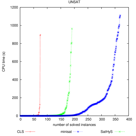
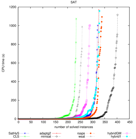
Figure 3: Crafted instances

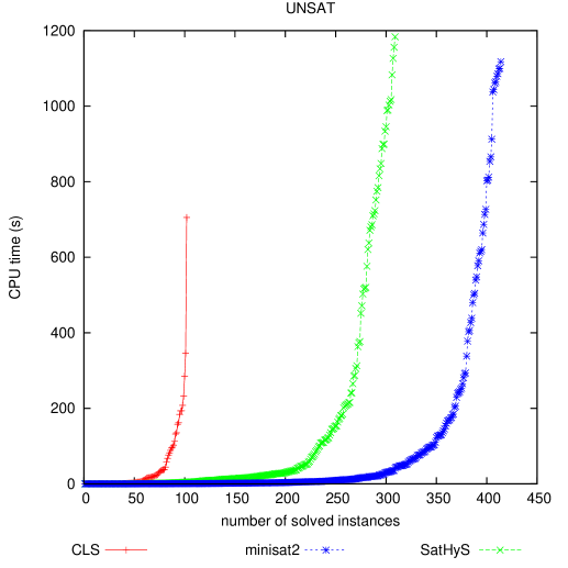
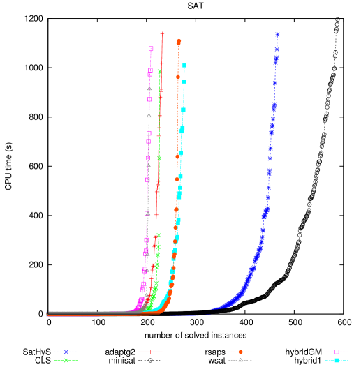
Figure 4: Industrial instances

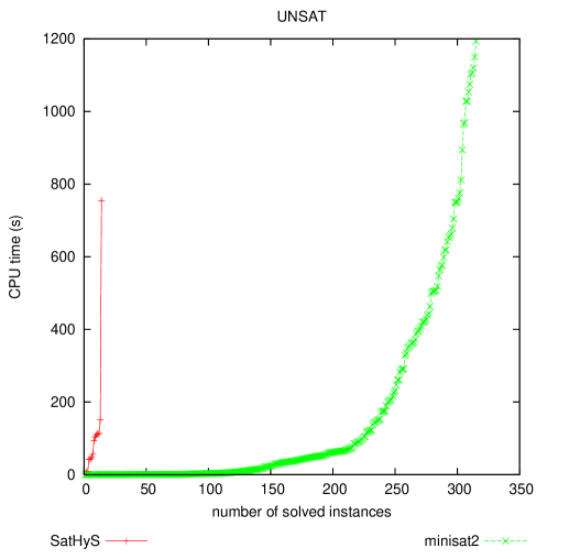
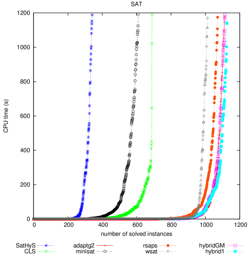
Figure 5: Random instances

The figures 3, 4 and 5 give the classical cactus plot. For each tested method, the X-axis corresponds to the number of formulas and the Y-axis corresponds to the time needed to solve them if they were ran in parallel. When a method does not appear in the curve, that means that this method is not able to solve instance of this instances category. In these figures, we have distinguished satisfiable and unsatisfiable instances for each categories.

7 Conclusion

In this paper a new integration of local search and CDCL based SAT solvers is introduced. This hybrid solver represents an original combination of both engines. The CDCL component can be seen as a new strategy for escaping from local minimum. This is achieved by the assignment of opposite literals from the falsified clause. In the case of satisfiable SAT instances, such assignments are supposed to behave like a tabu search approach, whereas for unsatisfiable ones, they try to focus on a small sub-part of the formula, which is minimally unsatisfiable (MUS). SatHyS, the resulting method, obtains very good results for a large category of instances. This new method can be improved in different ways. As it was pointed in the experimental section, our solver allows for more diversification and less intensification. First attempts have been done to correct this. Finally, we aim at designing a solver which would focuses only on an approximation of the MUS.

References

- [1]
- [2] B. B. & Fröhlich (2004): WalkSAT as an Informed Heuristic to DPLL in SAT Solving. Technical Report, CSE 573 : Artificial Intelligence.
- [3] A. Balint, M. Henn & O. Gableske (2009): A novel approach to combine a SLS- and DPLL-solver for the satisfiability problem. In: proceedings of SAT.
- [4] R. Battiti & M. Protasi (1997): Reactive search, a history-sensitive heuristic for MAX-SAT. J. Exp. Algorithmics 2, p. 2.
- [5] A. Biere, M. Heule, H. van Maaren & T. Walsh, editors (2009): Handbook of Satisfiability, Frontiers in Artificial Intelligence and Applications 185. IOS Press.
- [6] J. Crawford (1996): Solving Satisfiability Problems Using a Combination of Systematic and Local Search. In: Second Challenge on Satisfiability Testing organized by Center for Discrete Mathematics and Computer Science of Rutgers University.
- [7] M. Davis, G. Logemann & D. Loveland (1962): A machine program for theorem-proving. Communication of ACM 5(7), pp. 394–397.
- [8] N. Eén & A. Biere (2005): Effective Preprocessing in SAT Through Variable and Clause Elimination. In: proceedings of SAT. pp. 61–75.
- [9] N. Een & N. Sörensson (2003): An Extensible SAT-solver. In: proceedings of SAT. pp. 502–518.
- [10] E.Gregoire, B. Mazure & C. Piette (2006): Tracking MUSes and Strict Inconsistent Covers. In: Sixth ACM/IEEE International Conference on Formal Methods in Computer Aided Design(FMCAD’06). San Jose (USA), pp. 39–46.
- [11] H. Fang & W. Ruml (2004): Complete Local Search for Propositional Satisfiability. In: proceedings of AAAI. pp. 161–166.
- [12] L. Fang & M. Hsiao (2007): A new hybrid solution to boost SAT solver performance. In: proceedings of DATE. pp. 1307–1313.
- [13] F. Glover (1989): Tabu search - Part I. ORSA Journal of Computing , pp. 190–206.
- [14] E. Gregoire, B. Mazure & C. Piette (2006): Extracting MUSes. In: proceedings of ECAI. pp. 387–391.
- [15] E. Gregoire, B. Mazure & C. Piette (2007): Boosting a Complete Technique to Find MSS and MUS thanks to a Local Search Oracle. In: International Joint Conference on Artificial Intelligence(IJCAI’07). Hyderabad (India), pp. 2300–2305.
- [16] E. Gregoire, B. Mazure & C. Piette (2007): Local-Search Extraction of MUSes. Constraints 12(3), pp. 325–344.
- [17] D. Habet, C.M. Li, L. Devendeville & M. Vasquez (2002): A Hybrid Approach for SAT. In: Principles and Practice of Constraint Programming - CP 2002, 8th International Conference, CP 2002, Ithaca, NY, USA, September 9-13, 2002, Proceedings. pp. 172–184.
- [18] W. Havens & B. Dilkina (2004): A Hybrid Schema for Systematic Local Search. In: Canadian Conference on AI. pp. 248–260.
- [19] E. Hirsch & A. Kojevnikov (2005): UnitWalk: A new SAT solver that uses local search guided by unit clause elimination. Annals of Mathematical and Artificial Intelligence 43(1), pp. 91–111.
- [20] H. Hoos & T. Stützle (2004): Stochastic Local Search: Foundations and Applications. Morgan Kaufmann / Elsevier.
- [21] J. Huang (2007): The Effect of Restarts on the Efficiency of Clause Learning. In: proceedings of IJCAI. pp. 2318–2323.
- [22] F. Hutter, D. Tompkins & H. Hoos (2002): Scaling and Probabilistic Smoothing: Efficient Dynamic Local Search for SAT. In: proceedings of CP. pp. 233–248.
- [23] N. Jussien & O. Lhomme (2000): Local Search with Constraint Propagation and Conflict-Based Heuristics. In: AAAI/IAAI. pp. 169–174.
- [24] F. Letombe & J. Marques-Silva (2008): Improvements to Hybrid Incremental SAT Algorithms. In: proceedings of SAT. pp. 168–181.
- [25] C.M. Li, W. Wei & H. Zhang (2007): Combining Adaptive Noise and Look-Ahead in Local Search for SAT. In: proceedings of SAT. pp. 121–133.
- [26] B. Mazure, L. Saïs & E. Grégoire (1995): TWSAT : a new local search algorithm for SAT : performance and analysis. In: Proceedngs of the Workshop CP95 on Solving Really Hard Problems. pp. 127–130.
- [27] B. Mazure, L. Saïs & E. Grégoire (1998): Boosting Complete Techniques Thanks to Local Search Methods. Ann. Math. Artif. Intell. 22(3-4), pp. 319–331.
- [28] M. Moskewicz, C. Madigan, Y. Zhao, L. Zhang & S. Malik (2001): Chaff: Engineering an Efficient SAT Solver. In: proceedings of DAC. pp. 530–535.
- [29] B. Selman & H. Kautz (1993): An Empirical Study of Greedy Local Search for Satisfiability Testing. In: proceedings of AAAI. pp. 46–51.
- [30] B. Selman, H. Kautz & B. Cohen (1994): Noise Strategies for Improving Local Search. In: proceedings of AAAI. pp. 337–343.
- [31] B. Selman, H. Kautz & D. McAllester (1997): Ten Challenges in Propositional Reasoning and Search. In: proceedings of IJCAI. pp. 50–54.
- [32] L. Zhang, C. Madigan, M. Moskewicz & S. Malik (2001): Efficient Conflict Driven Learning in Boolean Satisfiability Solver. In: proceedings of ICCAD. pp. 279–285.