Alternative Fourier–series approach to nonlinear oscillations

Abstract

We propose an alternative approach that avoids the nonlinear equations for the Fourier coefficients that appear in the method of harmonic balance. We apply it to two simple illustrative examples.

1 Introduction

Since one–dimensional nonlinear oscillators are treated as simple pedagogical examples in many standard textbooks[1, 4, 2, 3, 5] one is tempted to believe that they are trivial problems. However, from time to time there appears to be a renewed interest in them as shown by a recent unbelievable article[6]. The equations of motion for the simplest nonlinear oscillators are suitable for illustrating the application of several approximate methods that include various forms of perturbation theory, variational approaches, Fourier expansions, etc.[1, 4, 2, 3, 5].

The method of harmonic balance[2], which is based on the Fourier expansion of the solution of a periodic nonlinear oscillator, yields accurate results but requires the solution to a rather complicated system of nonlinear equations for the expansion coefficients. It is not that difficult to select the physical solution of a nonlinear equation in one variable, but the problem becomes increasingly complicated as the number of equations and variables increases (specially if there are many unwanted solutions besides the physical one). The purpose of this communication is to propose a simpler approach that avoids the nonlinear system of equations for the Fourier coefficients. It is based on a systematic generalization of the approach proposed by Ren and He[6] in a paper plagued by errors and misconceptions[7]. In Sec. 2 we develop the method and in Sec. 3 we apply it to two simple but nontrivial illustrative examples. Finally, in Sec. 4 we discuss the advantages and limitations of the approach.

2 The method

Consider the dimensionless equation of motion for a nonlinear oscillator

$$u^{\prime\prime}(t)+f[u(t)]=0,\,u(0)=A,\,u^{\prime}(0)=0$$ (1)

where $u(t)$ is the displacement from equilibrium and the prime indicates differentiation with respect to the independent variable $t$. For simplicity we assume that the force $-f(u)$ is an odd function of the displacement: $f(-u)=-f(u)$ and that the motion is bounded with a period $T=2\pi/\omega$, where $\omega$ is the angular frequency. The potential–energy function $V(u)$ ($f(u)=dV(u)/du$) is, consequently, an even function of the displacement ($V(-u)=V(u)$). Such a symmetry and the initial conditions determine that $u(T/4)=0$ and therefore we can restrict our calculations to the interval $0\leq t\leq T/4$ where $A\geq u(t)\geq 0$. Obviously, if we know $u(t)$ in this interval then we know it for all values of $t$.

If we try to solve the equation of motion (1) by means of a truncated Fourier–series expansion

$$u^{[N]}(t)=\sum_{j=1}^{N}A_{j}\cos[(2j-1)\omega t]$$ (2)

and the method of harmonic balance[2] then we are led to a system of nonlinear equations for the expansion coefficients $A_{j}$. In what follows we propose a simple strategy that avoids such a problem. Notice that the ansatz (2) satisfies $u^{[N]}(T/4)=0$.

If we define $u^{(2n)}(t)=d^{2n}u(t)/dt^{2n}$, $u^{(0)}(t)=u(t)$ then we can write the set of equations $u^{(2n)}(0)=G_{n}(A),\,n=0,1,\ldots$, where $G_{0}(A)=A$, $G_{1}(A)=-f(A)$, $G_{2}(A)=f(A)f^{\prime}(A)$, etc. Substitution of Eq. (2) into the left–hand side of these equations for $n=0,1,\ldots,N-1$ leads to the linear system of equations

$$\sum_{j=1}^{N}(2j-1)^{2n}\omega^{2n}A_{j}=G_{n}(A),\,n=0,1,\ldots,N-1$$ (3)

that gives us the coefficients $A_{j}$ in terms of the amplitude $A$. The matrix of this system of equations is the transpose of a Vandermonde one and therefore its determinant is nonzero.

If we now integrate the equation of motion (1) twice and take into account the initial conditions we have

$$u(t)=A-\int_{0}^{t}\int_{0}^{t^{\prime}}f(u(t^{\prime\prime}))\,dt^{\prime\prime}\,dt^{\prime}$$ (4)

that we can apply iteratively. Here we carry out only one iteration

$$\tilde{u}^{[N]}(t)=A-\int_{0}^{t}\int_{0}^{t^{\prime}}f(u^{[N]}(t^{\prime\prime}))\,dt^{\prime\prime}\,dt^{\prime}$$ (5)

and obtain the period from the resulting approximate solution $\tilde{u}^{[N]}(t)$ and the condition derived above:

$$\tilde{u}^{[N]}(T/4)=0$$ (6)

For $N=1$ we simply have $u^{[1]}(t)=A_{1}\cos(\omega t)$ and $A_{1}=A$ from the only equation in (3). The system of equations (3) with $N=2$ yields

$$A_{1} = \frac{9A\omega^{2}-f(A)}{8\omega^{2}}$$

$$A_{2} = \frac{f(A)-A\omega^{2}}{8\omega^{2}}$$ (7)

These two approaches of first ($N=1)$ and second ($N=2$) order are sufficiently accurate as suggested by the examples below.

If the force is not an odd function of the displacement then we choose the ansatz $u^{[N]}(t)=A_{0}+A_{1}\cos(\omega t)+A_{2}\cos(2\omega t)+\ldots+A_{N}\cos(N\omega t)$, which should satisfy $u^{[N]}(0)=A$ and $u^{[N]}(T/2)=B$, and resort to the independent condition $\tilde{u}^{[N]}(T/2)=B$, where $B$ is the other turning point.

3 Examples

Our first example is one of the most widely studied nonlinear oscillators: the Duffing equation given by the function[1, 4, 2, 3, 5]

$$f(u)=u+\epsilon u^{3}$$ (8)

It is not difficult to prove that $\rho=\epsilon A^{2}$ is the relevant parameter of the model. That is to say, $u(t)/A$ and other properties of the system, like, for example, the period, depend on $A$ and $\epsilon$ only through $\rho$ and not separately or in other combinations.

In the first approximation we derive the period[6]

$$T^{[1]}(\rho)=\frac{6\pi}{\sqrt{7\rho+9}}$$ (9)

In order to verify its accuracy for large values of $\rho$ we recall that the exact period satisfies

$$\lim_{\rho\rightarrow\infty}\sqrt{\rho}T(\rho)=T_{\infty}=7.416298709$$ (10)

The approximate expression (9) yields the reasonable estimate

$$\lim_{\rho\rightarrow\infty}\sqrt{\rho}T^{[1]}(\rho)=T_{\infty}^{[1]}\approx 7.12$$ (11)

For small values of $\rho$ we have

$$T(\rho)=2\pi-\frac{3\pi\rho}{4}+\frac{57\pi\rho^{2}}{128}+\ldots$$ (12)

and

$$T^{[1]}=2\pi-\frac{7\pi\rho}{9}+\ldots$$ (13)

We appreciate that $T^{[1]}(\rho)$ does only give us the leading term of the small–$\rho$ series.

For $N=2$ we easily obtain

$$125T^{8}\rho\left(\rho+1\right)^{3}-7656\pi^{2}T^{6}\rho\left(\rho+1\right)^{2}+120\pi^{4}T^{4}\left(\rho+1\right)\left(1607\rho+735\right)$$

$$-64\pi^{6}T^{2}\left(48851\rho+55125\right)+12700800\pi^{8}=0$$ (14)

The approximate period is given by the only real root $T^{[2]}(\rho)$ that satisfies $T^{[2]}(0)=2\pi$. It is clear that we have not avoided the nonlinear nature of the problem completely but we have reduced it to a an equation with just one variable which simplifies the task of choosing the physical solution.

Without difficulty we derive the following expression for the approximation of second order to $T_{\infty}$

$$125T_{\infty}^{8}-7656\pi^{2}T_{\infty}^{6}+192840\pi^{4}T_{\infty}^{4}-3126464\pi^{6}T_{\infty}^{2}+12700800\pi^{8}=0$$ (15)

from which we obtain $T_{\infty}^{[2]}\approx 7.44$ that is in fact more accurate than $T_{\infty}^{[1]}$.

The Taylor expansion of $T^{[2]}(\rho)$ about $\rho=0$

$$T^{[2]}(\rho)=2\pi-\frac{3\pi\rho}{4}+\frac{1431\pi}{3200}+\ldots$$ (16)

exhibits the first two terms of the exact small–$\rho$ series.

Fig. 1 shows the exact period and the two approximations just derived for small and moderate values of $\rho$. We appreciate that $T^{[2]}(\rho)$ is more accurate than $T^{[1]}(\rho)$ for all values of $\rho$ as expected from the analytic results derived above. It is encouraging that the accuracy of the method increases notoriously with the order and that just the lowest two approximations are in good agreement with the exact result.

Our second example is given by

$$f(u)=u+\epsilon|u|u$$ (17)

and we realize that the relevant parameter is $\rho=\epsilon A$. This problem is as simple as the preceding one and we easily obtain $T_{\infty}=6.869261369$.

A straightforward calculation shows that the approximate method outlined in Sec. 2 yields

$$T^{[1]}(\rho)=\frac{8\pi}{\sqrt{\rho(\pi^{2}+4)+16}}$$ (18)

and $T_{\infty}^{[1]}\approx 6.75$ is a reasonable estimate of the exact large–$\rho$ limit. These results were obtained by Ren and He[6].

For the small–$\rho$ series we have

$$T(\rho)=2\pi-\frac{8\rho}{3}+\ldots$$ (19)

and

$$T^{[1]}(\rho)=2\pi-\frac{\pi(\pi^{2}+4)\rho}{16}+\ldots$$ (20)

For the second approximation we have

$$T^{6}\rho(\rho+1)^{2}(9\pi^{2}-16)-8\pi^{2}T^{4}(\rho+1)[\rho(45\pi^{2}-16)+256]$$

$$+16\pi^{4}T^{2}[\rho(369\pi^{2}+1136)+5120]-294912\pi^{6}=0$$ (21)

and the expression for the large–$\rho$ limit

$$T_{\infty}^{6}(9\pi^{2}-16)+8\pi^{2}T_{\infty}^{4}(16-45\pi^{2})+16\pi^{4}T^{2}(369\pi^{2}+1136)-294912\pi^{6}=0$$ (22)

The estimate $T_{\infty}^{[2]}\approx 6.866$ is more accurate than $T_{\infty}^{[1]}$.

The small–$\rho$ expansion is also more accurate

$$T^{[2]}(\rho)=2\pi-\frac{\pi(9\pi^{2}+20)\rho}{128}+\ldots$$ (23)

but neither $T^{[1]}$ nor $T^{[2]}$ gives more than the leading term exactly.

Fig. 2 shows the exact period and the approximations of first and second order for small and moderate values of $\rho$. Once again we appreciate that the accuracy of the method increases with the order.

4 Conclusions

We have developed a straightforward systematic approach for the calculation of the period of simple nonlinear oscillators. It is particularly useful if we can integrate the equation (5) analytically which we easily do when $f(u)$ is a polynomial or when a few terms of the Taylor series about $u=0$ give a reasonable approximation.

Although present approach becomes increasingly complicated with the order, we think that its equations are always considerably simpler than those coming from the method of harmonic balance[2].

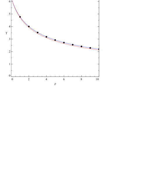
Figure 1: Period for the Duffing oscillator. Circles, dashed and solid lines stand for exact, first and second approximations, respectively

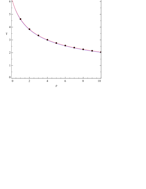
Figure 2: Period for the discontinuous oscillator. Circles, dashed and solid lines stand for exact, first and second approximations, respectively

References

- [1] A. H. Nayfeh, ”Perturbation Methods,” (Joh Wiley & Sons, New York, 1973).
- [2] A. H. Nayfeh and D. T. Mook, Nonlinear Oscillations, (John Wiley & Sons, New York, 1979).
- [3] A. H. Nayfeh, Introduction to Perturbation Techniques, (John Wiley & Sons, New York, 1981).
- [4] C. M. Bender and S. A. Orszag, Advanced Mathematical Methods for Scientists and Engineers, (McGraw-Hill, New York, 1978).
- [5] S. H. Strogatz, Nonlinear Dynamics and Chaos, (Perseus Books, Reading, Massachusetts, 1994).
- [6] Z-F Ren and J-H He, Phys. Lett. A 373 (2009) 3749-3752.
- [7] F. M. Fernández, On a simple approach to nonlinear oscillators, arXiv:0910.0600v1 [math-ph].