Entanglement in a spin system with inverse square statistical interaction

Abstract

We investigate the entanglement content of the ground state of a system characterized by effective elementary degrees of freedom with fractional statistics. To this end, we explicitly construct the ground state for a chain of $N$ spins with inverse square interaction (the Haldane-Shastry model) in the presence of an external uniform magnetic field. For such a system at zero temperature, we evaluate the entanglement in the ground state both at finite size and in the thermodynamic limit. We relate the behavior of the quantum correlations with the spinon condensation phenomenon occurring at the saturation field.

I Introduction

Quantum states of interacting many body systems are inherently entangled. This simple statement has motivated a wide physics community to study, in the light of quantum information theory, models typically explored in quantum statistical mechanics amicorep . Besides the motivation of the crucial role played by the entanglement as a resource for quantum computation protocols, the promise is to acquire a deeper understanding of the physical systems themselves, with possible spin off on open problems in condensed matter. There are indications that, while local interactions are possibly the most common mechanisms leading to non local correlations, also statistics can produce entanglement. Indeed, because of the symmetrization constraints, most generically identical particles are not in a product state. Even though the resulting many body wave function cannot lead to genuine entangled state because of the lack of the tensor product structure in Fock spaces Ghirardi , Vedral Vlatko-fermions demonstrated that a free fermion gas enjoys spin entanglement on distances of the order of the inverse Fermi momentum; on the contrary, no such kind of entanglement has been found for the polarizations of identical bosons. An alternative route to capture non local correlations in the states of identical particles was pursued by Zanardi and coworkers through the so called mode-entanglement, directly defined in the Fock space Zanardi . As a basic support to this point of view, one can argue that separable states in the dual space correspond to configurationally entangled states. Furthermore, in favor of such ‘statistics entanglement’, it should be noticed that several protocols have been suggested to exploit it for computational purposes Cavalcanti .

In this paper, we deal with statistics in a one dimensional interacting many particle system. In one dimension, statistics is peculiar as particles need to scatter each other in order to exchange their position. Accordingly, one dimensional statistics can be formulated as a boundary condition for the many-body wave function in the configurational space Les-Houches1999 . In this context, particularly relevant are the Calogero-Sutherland models (CSM)s, i.e., quantum mechanical models in one dimension where the interaction among particles is inversely proportional to the square of their distance. Indeed, such models can be regarded as describing a gas of identical free particles with fractional statistics Haldane-exclusion ; Calogero-statistics , which has made them relevant in the understanding of the fractional quantum Hall effect.

The main motivation of our work is to investigate the kind of entanglement emerging from fractional statistics. We note that, because of the lack of any tensor product structure, the entanglement between particles with fractional statistics has not been fully quantified yetpartitions . We concentrate on the spin entanglement emerging from quasi-particles with fractional statistics. To rely on some tensor product structures of the underlying Hilbert space hosting the quantum system, we consider the Haldane-Shastry haldaneshastry model (HSM): an anti-ferromagnetic spin-$1/2$ chain with inverse square exchange interaction among the spins.

Also the HSM (in the dual space) can be interpreted as an ideal gas with fractional statistics Haldane-ideal . The connection with the CSM can be put on firm grounds following the scheme developed by Polychronakos; namely, first introducing some internal degrees of freedom into the CS model and then employing the so called ‘freezing trick’, to fix the particle positions toadd1 . As can be understood by a direct inspection of the eigenstates of the two models, it is worth mentioning that the correspondence between the CSM and the HSM holds only for a well-defined value of the parameter characterizing the statistics of the excitations in the CSM, identifying a ‘semion’ gas (i.e., a gas of particles with statistics half than the Fermi statistics). One of the most spectacular evidences that the HSM is indeed an ideal gas of semions is provided by the response of the system to a local perturbation: it can be proved that a single spin flip causes the creation of a pair of collective excitations (spinons). Higher ‘angular momenta’ excitations are generated by two or more spin flips haldanemagnetic .

In the present paper, we study the entanglement in the ground state of the HSM in an external magnetic field. In fact, the applied magnetic field causes a certain number of spin flips to occur in the ground state: this allows us to study quantum correlations in the presence of spinon condensation. We shall demonstrate that the divergence of the spinon ’Fermi’ wavelength occurring when all the spinons in the system actually condense (saturation field), a characteristic trait of the semionic statistics, causes a divergence of the entanglement length. We also note that in our work we study the interplay between the range of local interaction and the range of the entanglement. We eventually find that a specific pattern of entanglement characterizes the system with a finite range interaction.

The paper is organized as follows: in the following section, we introduce the model and explicitly construct its ground state as function of the magnetic field; in Sect. III, we employ the single- and two-spin ground state averages, computed in Appendix A to evaluate various entanglement measures. Finally, Sect. IV contains some concluding remarks.

II The model

The Haldane-Shastry (HS) Hamiltonian haldaneshastry describes a one-dimensional spin-$1/2$ chain wrapped around a circle of unit radius, with an anti-ferromagnetic interaction whose strength is inversely proportional to the square of the chord between the corresponding sites. When the model is placed in an external uniform magnetic field $h$, its Hamiltonian is given by

$$H=\frac{2\pi^{2}J}{N^{2}}\>\sum_{\alpha\neq\beta=0}^{N-1}\>\frac{{\bf S}_{\alpha}\cdot{\bf S}_{\beta}}{|z_{\alpha}-z_{\beta}|^{2}}+h\sum_{\alpha=0}^{N-1}S_{\alpha}^{z}\>\>\>\>.$$ (1)

In Eq. (1), ${\bf S}_{\alpha}$ is the spin operator and $z_{\alpha}$ the spin coordinate of the site $\alpha=0,1,\ldots,N-1$, with $N$ the total number of spins. Periodically boundary conditions $z_{\alpha}=z_{\alpha+N}$, and ${\bf S}_{\alpha}={\bf S}_{\alpha+N}$, allow to parameterize the positions on the circle by the $N^{\rm th}$ roots of the unity $z_{\alpha}=e^{2\pi i\alpha/N}$. For $h=0$, the ground state of the system is a non-degenerate spin liquid with $0$ total spin (a spin singlet) haldaneshastry . At zero field, flipping a spin in the ground state corresponds to creating a (fully polarized) pair of spin-$1/2$ collective excitations faddeev , dubbed “spinons” by Haldane Haldane-exclusion . The spinons keep their integrity when scattered off each other, so that they can be thought of as true quantum particles, despite their collective nature. Any time one more spin is flipped, an additional spinon pair is created in the state of the system; flipping $K/2$ spins is, thus, equivalent to creating a fully polarized $K$-spinon excited state. The Zeeman energy in Eq. (1) lowers the energy of the fully polarized states, since $h$ works like a chemical potential for the spinons. Thus, upon increasing the magnetic field the (even) number of spinons $K$ increases and one of the fully polarized $K$-spinon states becomes the ground state of the system. This state can be written as

$$|\Phi_{\rm gnd},K\rangle=\sum_{z_{1},\ldots,z_{M}}\>\Phi_{K}(z_{1},\ldots,z_{M})\>|z_{1},\ldots,z_{M}\rangle\>\>\>\>,$$ (2)

where $z_{1},\ldots,z_{M}$ denote the positions of the $\uparrow$-spins in the state, the remaining ones pointing downwards. In Eq. (2), the number of $\uparrow$-spins is given by $M=(N-K)/2$, where $K$ is the number of condensed $\downarrow$-spinons in the ground state; the state $|z_{1},\ldots,z_{M}\rangle$ is understood to be equal to $|z_{1},\ldots,z_{M}\rangle=S_{1}^{+}\ldots S_{M}^{+}\>|\downarrow\rangle^{\otimes N}$ and the amplitude $\Phi_{K}(z_{1},\ldots,z_{M})$ has the form

$$\Phi_{K}(z_{1},\ldots,z_{M})=\left[\frac{N^{M}(2M)!}{2^{M}}\right]^{-\frac{1}{2}}\>\prod_{t=1}^{M}z_{t}^{1+K/2}\>\prod_{i<j=1}^{M}(z_{i}-z_{j})^{2}\>\>\>\>.$$ (3)

The number of condensed spinons is determined by the value of the external field. In order to find out how $K$ increases with $h$, one has first to calculate the energy $E_{\rm gnd}[N,K,h]$ of the state $|\Phi_{\rm gnd},K\rangle$, as a function of $K$ and $h$ at fixed $N$, and then to determine the value of $K$ that minimizes $E_{\rm gnd}[N,K,h]$, at fixed $h$. $E_{\rm gnd}[N,K,h]$ can be obtained, for example, by a straightforward generalization of the approach developed in Ref. bgl : since $\Phi_{K}(z_{1},\ldots,z_{M})$ is a homogeneous polynomial of $z_{1},\ldots,z_{M}$, the summations over spin indices, contained in the expectation value $\langle\Phi_{\rm gnd},K|H|\Phi_{\rm gnd},K\rangle$, are replaced by derivative operators that are understood to act onto the analytic extension of $\Phi_{K}(z_{1},\ldots,z_{M})$, in which the spin coordinates are allowed to take any value on the unit circle. After computing the derivatives, the variables $z_{1},\ldots,z_{M}$ are constrained back to the lattice sites. The ground state energy is then the minimum energy of a $K$-spinon condensate at finite $h$; it can be expressed as

$$E_{\rm gnd}[N,K,h]=E[q_{1}(M),\ldots,q_{\frac{K}{2}}(M),q_{\frac{K}{2}+1}(0),\ldots q_{K}(0)]-h\frac{K}{2}\;,$$ (4)

in which

$$E[\ldots,q_{\ell}(m_{\ell}),\ldots]=-\frac{\pi^{2}J(N^{2}+5)}{24N}+\frac{1}{2}\sum_{\ell=1}^{M}\left[J\left(\frac{\pi}{2}\right)^{2}-Jq_{\ell}(m_{\ell})^{2}+\frac{\pi^{2}J}{4N^{2}}\right]\>\>\>\>.$$ (5)

is the energy part associated to the bare HS Hamiltonian, and

$$q_{\ell}(m_{\ell})=\frac{\pi}{2}-\frac{2\pi}{N}\left[m_{\ell}+\frac{1}{2}\left(K-\ell+\frac{1}{2}\right)\right]\;\;\;\;$$ (6)

denote the spinon (pseudo) momenta with $0\leq m_{1}\leq\ldots\leq m_{K}\leq M$.

According to Eqs. (4)-(6), the minimum energy $K$-spinon fully polarized state is realized for $m_{1}=\ldots=m_{K/2}=M$ and $m_{K/2+1}=\ldots=m_{K}=0$, which corresponds to the condensing spinons being equally distributed at the ends of the single-spinon Brillouin zone, as depicted in Fig.1.

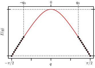
Figure 1: Single-spinon level occupancy corresponding to the state $|\Phi_{\rm gnd},K\rangle$. The spinons symmetrically populate low-energy states around the corners of the Brillouin zone (which ranges from $-\pi/2$ to $\pi/2$). The corresponding “spinon Fermi surface” is composed by two disconnected ’Fermi’ points (the largest values of the momenta at which we can create a spin pair), at $\pm q_{0}=\pm\frac{\pi}{2}\left(1-\frac{K}{M}\right)$.

When all the spins in $|\Phi_{\rm gnd},K\rangle$ are polarized, that is, when $K=N$, the ground state of the system is given by the simple factorized state $|\Phi_{\rm gnd},N\rangle=|\downarrow\rangle^{\otimes N}$. In the language of spinons, $|\Phi_{\rm gnd},N\rangle$ corresponds to a state with the single-spinon Brillouin zone completely filled. In fact, the “saturated state” $|\Phi_{\rm gnd},N\rangle$ becomes the ground state of the system as soon as $h>h_{s}$, where $h_{s}$ is the “saturation field” (to be estimated below). The interval $0\leq h\leq h_{s}$ is, therefore, divided into $N/2$ regions labelled by the number of condensing spinons. The $n^{\rm th}$ region, with $2n$ spinons ($n=0,\ldots,N/2-1$), ends with the energy crossing between $E_{\rm gnd}[N,K=2n,h]$ and $E_{\rm gnd}[N,K=2n+2,h]$. The width of each interval becomes smaller, and the set of crossing points becomes denser, as the number of spins increases, which gives rise to a quantum instability similar to those found for the Dicke and the $XX$ models plastina .

Let $K[N,h]$ be the number of condensing spinons, obtained with the minimization procedure outlined above. The variation of $K[N,h]$ with respect to $h/J$ for different values of $N$ is reported in Fig. 2A, where it is shown that, for large enough $N$, the steps in $K[N,h]$ are smoothed down. This implies that the spinon density $K[N,h]/N$, shown in Fig. 2B, can be approximated with a continuum function $\rho_{K}(N,h)$, whose dependence on $h$ at fixed $N$ is given by

$$\rho_{K}(N,h)=1-\sqrt{1-\frac{4h}{\pi^{2}J}+\frac{4}{3N^{2}}}\>\>\>\>.$$ (7)

It is worthwhile noticing that $\rho_{K}(N,h)$ is independent of $N$, as $N\to\infty$, which is also displayed in Fig. 2B. The value of the saturation field $h_{s}$ can be derived from Eq. (7), by requiring that $\rho_{K}(N,h)=1$, for $h>h_{s}$. As a result, one obtains $h_{s}\approx\pi^{2}J\left(\frac{1}{4}+\frac{1}{3N^{2}}\right)$, which, for large enough $N$ ($\geq 10$), gives $h_{s}\approx\pi^{2}J/4$. Accordingly, the number of condensed spinons as a function of the external field is given by

$$K[N,h]=\biggl{\{}\begin{array}[]{l}N-\frac{2N}{\pi}\sqrt{\frac{h_{s}-h}{J}}\>\>{\rm for}\>h\leq h_{s}\\ N\>\>\>{\rm for}\>h>h_{s}\end{array}\>\>\>\ .$$ (8)

This can be regarded as a “thermodynamic limit formula”, which is confirmed by the plots of Fig. 2B.

III Ground state entanglement

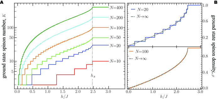
Figure 2: A: Number of condensed spinons, $K[N,h]$, vs. $h/J$, for different values of $N$ ranging from $10$ to $400$. B: Density of condensed spinons $\rho[N,h]$, vs. $h/J$, for $N=20$ and $N=100$; the thermodynamic expression (7), holding exactly for $N\to\infty$, is also shown for comparison.

This section is concerned with the evaluation of two kinds of entanglement measures, both depending on the external magnetic field and on the number of spins. One of these is the one-tangle $\tau_{1}(N,h)$, which quantifies the amount of entanglement shared by each spin with the rest of the system; the other is the concurrence of any pair of spins $C(N,h,r)$ that also depends on the relative distance between the spin sites $r=\alpha-\alpha^{\prime}$ ($\alpha\neq\alpha^{\prime}=0,\ldots,N-1$), because of the translational invariance of the system (see also CKW ).

Using the concurrence, the two-tangle $\tau_{2}(N,h)=\sum_{r}C^{2}(N,h,r)$ and then the entanglement ratio $R(N,h)=\tau_{2}(N,h)/\tau_{1}(N,h)$ will be evaluated. They will provide information about the fraction of entanglement shared by pairs with respect to the total (i.e. both bipartite and multipartite) entanglement to which each spin participates. In order to evaluate these entanglement measures, the mean values of the spin operators and of the two-spin correlation functions are needed on the state $|\Phi_{\rm gnd},K\rangle$.

The technical steps required to obtain these quantities are reported in the appendix A, where their explicit expressions are given, and where the thermodynamic limit is thoroughly discussed. In particular, all of the one- and two-spin properties can be determined analytically for any value of the external field $h$, and for any given number of spins $N$, except for the longitudinal correlation function. The latter is obtained numerically at specific values of $h$ (see appendix A for the details).

III.1 One-tangle

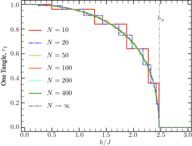
Figure 3: One-tangle $\tau_{1}$ vs. $h/J$ for several values of $N$. For $N>100$, the plot is well fitted by the thermodynamic limit formula (11).

To compute the one-tangle, one needs to obtain the average value of the three cartesian components of each spin $S^{j}_{\alpha}$, with $j=x,y,z$, on the ground state amicorep . Since the applied magnetic field does not break the rotational symmetry around the $z$-axis, one gets

$$\langle\Phi_{\rm gnd},K|S^{x}_{\alpha}|\Phi_{\rm gnd},K\rangle=\langle\Phi_{\rm gnd},K|S^{y}_{\alpha}|\Phi_{\rm gnd},K\rangle=0\;\;\;,$$ (9a)

and

$$\langle\Phi_{\rm gnd},K|S^{z}_{\alpha}|\Phi_{\rm gnd},K\rangle=-\frac{K[N,h]}{2N}\equiv-\bar{m}\;\;\;,$$ (9b)

where $$-\bar{m}$$ coincides with the average magnetization of the ground state.

Consequently, the one-tangle has the form

$$\tau_{1}(N,h)=1-4|\langle\Phi_{\rm gnd},K|S^{z}_{\alpha}|\Phi_{\rm gnd},K\rangle|^{2}=1-\frac{K[N,h]^{2}}{N^{2}}\>\>\>\>.$$ (10)

In Fig. 3, $\tau_{1}$ is shown as a function of $h/J$, for different values of $N$. Similarly to the plots shown in Fig. 2B, it is worthwhile noticing that, for $N>100$, the curves are well approximated by the analytical formula

$$\tau_{1}(N\to\infty,h)=\biggl{\{}\begin{array}[]{l}\frac{4}{\pi}\sqrt{\frac{h_{s}-h}{J}}-\frac{4}{\pi^{2}}\left(\frac{h_{s}-h}{J}\right)\;\;\;,\;\;{\rm for}\>h\leq h_{s}\\ 0\;\;\;,\;\;{\rm for}\>h>h_{s}\end{array}\>\>\>\>,$$ (11)

obtained in the thermodynamic limit, and yielding the dominant behavior

$$\tau_{1}(N\to\infty,h\rightarrow h_{s}^{-})\sim\left(h_{s}-h\right)^{1/2}\>\>\>\>.$$ (12)

III.2 Bipartite entanglement

By taking into account the symmetries of the Hamiltonian, it is easy to show that the two spin reduced density matrix has the so called $X$-form and that the concurrence $C(N,h,r)$ can be expressed in terms of the two-point correlation functions

$$g^{jj^{\prime}}(N,h,r)=\langle\Phi_{\rm gnd},K|S_{\alpha=0}^{j}S_{\alpha^{\prime}=r}^{j^{\prime}}|\Phi_{\rm gnd},K\rangle\;\;\;,$$ (13)

in which $j,j^{\prime}=x,y,z$ amico . In particular, when two spins are at a distance $r$ from each other, one gets $C(N,h,r)={\rm max}\{0,C_{a}(N,h,r)\}$, where

$$C_{a}(N,h,r)=4\sqrt{[g^{xx}(N,h,r)]^{2}+[g^{xy}(N,h,r)]^{2}}-2\sqrt{[1/4+g^{zz}(N,h,r)]^{2}-\bar{m}^{2}}\>\>\>\>$$ (14)

denotes the antiparallel concurrence. Since the latter depends on the longitudinal spin-spin correlation function, $g^{zz}(N,h,r)$, its expression can be obtained analytically only in the range of $h$ for which such a function is is known (see appendix A), and is otherwise computed numerically.

For $h=0$, using $g^{jj}(N,h=0,r)\equiv g_{0}(r)$, for each $j=x,y,z$, and $g^{xy}(N,0,r)=0$, one obtains the zero-field concurrence:

$$C(N,0,r)={\rm max}\{0,4|g_{0}(r)|-2\sqrt{1/4+[g_{0}(r)]^{2}}\}\>\>\>\>.$$ (15)

An explicit evaluation shows that, for any $N$, $C_{a}(N,h=0,r)$ is always negative, except for the cases $r=1$ and $r=N-1$. The same property holds in the thermodynamic limit where $g_{0}(r)$ takes the expression: haldaneshastry

$$g_{0}(r)\approx\frac{(-1)^{r}}{16\pi}\>\int_{-\pi/2}^{\pi/2}\>dq_{\alpha}\>dq_{\beta}\>\frac{|q_{\alpha}-q_{\beta}|e^{-i(q_{\alpha}+q_{\beta})r}}{\sqrt{\pi^{2}/4-q_{\alpha}^{2}}\>\sqrt{\pi^{2}/4-q_{\beta}^{2}}}\>\>\>\>,$$ (16)

and the condition $C_{a}(N,h=0,r)>0$ is satisfied only for $r=1$. Therefore, for $h=0$, only the concurrence between spins lying onto nearest neighboring sites is different from zero, as it could be expected for an isotropic spin liquid state.

Due to the lack of an explicit analytical formula for $g^{zz}(N,h,r)$, the concurrence in the intermediate range $0<h<h_{s}$ needs to be computed numerically. A result in the whole range can be easily found in the case $N\leq 20$; in particular, Figs. 4A and 4B show the behavior of the concurrence vs. $h$, at fixed $r$, for $N=10$ and $N=20$, respectively. One clearly sees that the switching on of the magnetic field leads to an enlargement of the entanglement range, as $C(N,h,r)$ becomes positive also for $r>1$.

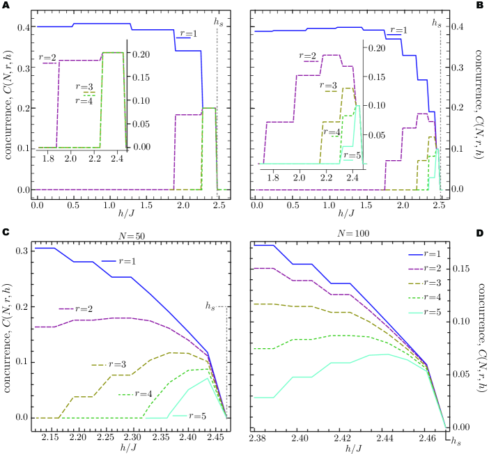
Figure 4: $C(N,h,r)$ vs. $h$ at fixed $r$ and for various values of $N$. Upon increasing $h$, $C(N,h,r=2)$ can be made $>0$, thus yielding nonzero second neighbor concurrence. At a higher value of $h$, $C(N,h,r\geq 3)$ becomes $>0$, as well.

For $N\geq 50$, it is still possible to determine $C(N,h,r)$ exactly but only at values of $h$ close to the saturation field. This is shown in plots of Figs. 4C and 4D, where the behavior of the concurrence near $h_{s}$ is shown for $N=50,100$ and $r=1-5$. In fact, when $h\sim h_{s}$, the leading contribution to $C(N,r,h)$ can be calculated by thermodynamic arguments, putting together the relationships (27) and (32) derived in the appendix A. For relevant values of $r$ ($r\neq 0,N$), one obtains

$$C_{a}(N\to\infty,h,r)=4q_{0}\left\{|\gamma(q_{0}r)|-\frac{1}{\pi}\sqrt{\left(1-\frac{2q_{0}}{\pi}\right){\cal F}[q_{0},r]+\left(\frac{2q_{0}}{\pi}\right)^{2}{\cal F}^{2}[q_{0},r]}\right\}\>\>\>\>,$$ (17)

where the functions $\gamma$ and ${\cal F}$ are also defined in the appendix A and $q_{0}$, the magnitude of the ‘Fermi momentum’ indicated in Fig. 1, can be expressed as $q_{0}=\frac{\pi}{2}(1-2\bar{m})$. As a result, one finds

$$C_{a}(N\to\infty,h\sim h_{s},r)\sim\sqrt{(h_{s}-h)/J}\>\Phi(q_{0},r)\>\>\>\>,$$ (18)

where $\Phi(q_{0},r)$ is a regular function of $q_{0},r$. In particular, at $h\to h_{s}$, one gets $q_{0}=0$ implying $\gamma(0)=\pi/2$ and ${\cal F}[q_{0}\to 0,r]=0$, as it will emerge from the discussion in the appendix A. Thus,

$$C_{a}(N\to\infty,h\to h_{s},r)=\frac{1}{\pi}\>\sqrt{\frac{h_{s}-h}{J}}+{\cal O}\left(\frac{h_{s}-h}{J}\right)\;\;\;\;,$$ (19)

independently of $r$. The remarkable collapse of the curves onto each other for $h\to h_{s}$, reported in Fig.5 for $r=1,2$ and for $N=10,20,50,100$, confirms the prediction of Eqs. (17), (19).

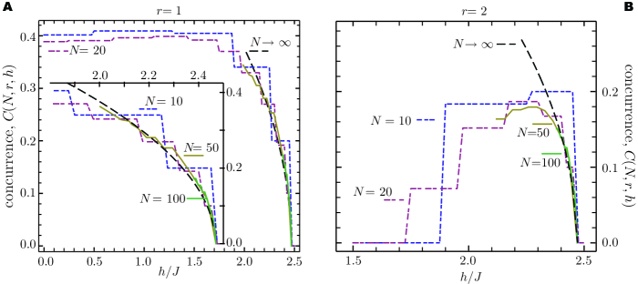
Figure 5: Behavior of $C(N,r,h)$ for $h\to h_{s}$ with $r=1$ (left panel) and $r=2$ (right panel) and for $N=10,20,50,100$, and $N\to\infty$ (thermodynamic limit). Upon increasing $h$, the entanglement range increases while at $h_{s}$ all the curves show the universal behavior of Eq. (19)

In general, one can say that by increasing the distance $r$, the concurrence $C(N,h,r)$ is different from zero only in a smaller and smaller region of the magnetic field and that the range of the bipartite entanglement, $r_{c}$, extends to the whole chain near the saturation point $h_{s}$. The behavior of $r_{c}$ vs $h/J$ is shown in Fig. 6. This is clearly reminiscent of what happens at factorization points luigipaola .

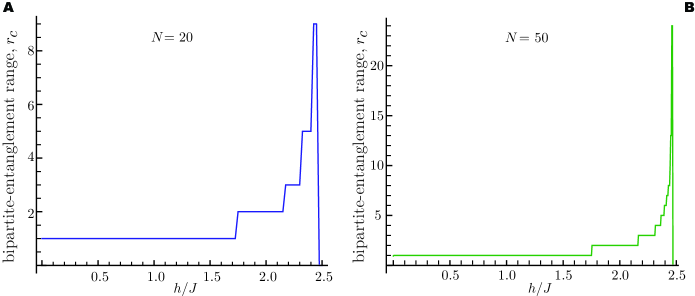
Figure 6: Behavior of the range of the bipartite entanglement vs $h/J$; as $h\to h_{s}$, all the spinons are entangled and $r_{s}\to N/2$

In accordance with this observation, we show below that near the saturation field, the bi-partite entanglement is dominant with respect to multi-partite ones, as it is the case for factorization points.

III.3 Two-tangle and entanglement ratio

In order to understand wether the entanglement stored in the ground state has a multi-partite rather than a bi-partite nature, we consider in this section the ratio between the two-tangle and the one-tangle defined above. Due to the monogamy relation for entanglement, this ratio is bound between zero (for purely multipartite correlations) and one (for bipartite entanglement) CKW .

We first focus on the two-tangle, that gives an overall measure of the bi-partite entanglement to which a given spin participate. It is defined by

$$\tau_{2}(N,h)=2\sum_{r=1}^{N/2}C(N,h,r)^{2}\text{,}$$ (20)

and its behavior with respect to the magnetic field is reported in Fig. 7A.

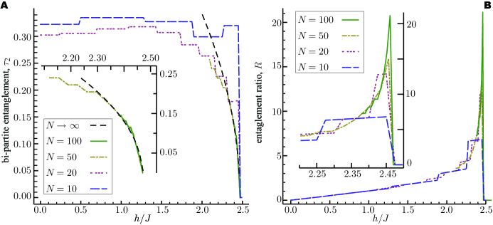
Figure 7: A: Two-tangle, $\tau_{2}$ as a function of the magnetic field. The black dashed line gives the limiting behavior reported in Eq.(21). B: Entanglement ratio as a function of the external field. The plot suggests that near the saturation point, $\tau_{2}$ dominates over $\tau_{1}$.

When $h\to h_{s}$, the limiting trend (black dashed line) is given by

$$\tau_{2}(N,h\rightarrow h_{s})\sim\left(h_{s}-h\right)^{\alpha},$$ (21)

with an exponent that we estimated, by fitting, to be $\alpha=0.50\pm 0.02$. This already implies that, near $h_{s}$, $\tau_{2}$ goes to zero as the one-tangle: $\tau_{1}\sim(h_{s}-h)^{0.5}$.

To better show this fact, we finally consider the entanglement ratio $R(N,h)=\tau_{2}(N,h)/\tau_{1}(N,h)$, whose behavior is reported in Fig. 7B. Near the saturation field, the limiting trend $R(N,h\to h_{s})\sim\left(h_{s}-h\right)^{\beta}$ has an exponent $\beta$ taking values smaller than $0.03$, which is consistent with the other estimates given above. More importantly, the plot shows that at $h\to 0$ the one-tangle dominates, whereas in the neighborhood of $h_{s}$ the entanglement is essentially bi-partite.

IV Concluding Remarks

Typical spin models considered so far to discuss the behavior of entanglement lie into two main categories: those with nearest neighbor interaction, such as the Ising model in a transverse field, and those with long range interaction with spins residing on a fully connected graph, such as the LMG model lmgnuovi or the uniaxial model vidal . In the former case, amicorep , bipartite entanglement decays quickly with the distance, and only nearest and next to nearest neighbor entanglement is found to survive. Notable exception are factorization points around which the concurrence is found to have an infinite range luigipaola . In collective spin models, on the other hand, the qubit-qubit entanglement is strictly zero in the thermodynamic limit, and its presence in the ground state is only due to finite size effects. In particular, the concurrence is found to scale as $(N-1)^{-1}$, where $N$ is the number of spins.

We have found that the inverse square (statistical) interaction among spins produces a quite different behavior of the entanglement as a function of the distance. In particular, we have shown that, in the absence of external magnetic field, $h=0$, the system only displays nearest neighbor concurrence, while the entanglement has essentially a multi-partite nature; while, by increasing $h$, the entanglement becomes essentially bi-partite and the range of the concurrence increases. For a large enough $h$, the spin system eventually saturates, entering a fully polarized phase described by a completely separable ground state. We have discussed in particular the behavior of the entanglement near this saturation point, both for a finite size system and in the thermodynamic limit. In particular, we found that the divergence of the range of the bipartite entanglement is governed by the same exponent ($|h-h_{s}|^{1/2}$) of the ordinary isotropic Heisenberg model, consistently with the fact that the latter belongs to the same universality class as the Haldane-Shastry model.

Since the inverse square interaction among spins in the HS model is essentially of statistical nature, the fact that the entanglement range tends to diverge near the saturation can be compared with the behavior of entanglement for other systems of indistinguishable free particles. As mentioned in the introductory section, the spin entanglement of a free electron gas is different from zero within a distance of the order of the Fermi wavelength. On the other hand, we have shown that in the presence of a large number of semions (i.e., near $h=h_{s}$), the range of the bipartite entanglement extends to comprise the entire system. This behavior is ultimately due to the fractional statistics: by increasing the value of the external field, more and more spinons can be added to the system with smaller and smaller momenta, starting from the edge of the Brillouin zone and going towards its center. This implies that the only length scale of the system is the ’Fermi’ wavelength $q_{0}^{-1}$, which, because of the semionic statistics, diverges when the saturation point is approached. In a sense, this behavior interpolates between the cases of entanglement among bosons and fermions. Free bosons can be always in a factorized state because there is no correlation between their relative distance and their polarization; for free fermions the range of bipartite entanglement between their spin is spatially limited to a finite Fermi length. For the semionic gas a Fermi length does exist, but it diverges at $h_{s}$. Therefore, because of their quantum statistics an overlap of the spinon wave functions (whose extension is roughly given by $\hbar/q_{0}$) can take place at $h_{s}$, ultimately making the saturation phenomenon a result of spinon condensation.

Appendix A Magnetization and Spin correlation functions on $|\Phi_{\rm gnd},K\rangle$

This appendix contains the one- and two-spin correlation functions on $|\Psi_{\rm gnd},K\rangle$. These are the basic bricks to build the single- and two-spin density matrices needed to evaluate the entanglement. When possible, the calculations are carried out analytically on a finite chain and the thermodynamic limit is systematically worked out by sending $N\to\infty$, while keeping $K/N$ constant. When exact analytical results are lacking, namely in the calculation of the longitudinal two spin correlation functions, the corresponding quantities have been evaluated numerically.

A.1 One-spin average values

Since $|\Phi_{\rm gnd},K\rangle$ is an eigenstate of $S^{z}=\sum_{\alpha=1}^{N}S_{\alpha}^{z}$, with total eigenvalue $-K/2$, one readily obtains $\langle\Phi_{\rm gnd},K|S_{\alpha}^{x}|\Phi_{\rm gnd},K\rangle=\langle\Phi_{\rm gnd},K|S_{\alpha}^{y}|\Phi_{\rm gnd},K\rangle=0$. Moreover, because of the translational invariance on the lattice, one also has

$$\langle\Phi_{\rm gnd},K|S_{\alpha}^{z}|\Phi_{\rm gnd},K\rangle=-\frac{1}{2}+M\sum_{z_{2},\ldots,z_{M}}|\Phi_{K}(1,z_{2},\ldots,z_{M})|^{2}=-\frac{K}{2N}\>\>\>\>.$$ (22)

The thermodynamic limit is defined as $N\to\infty$, with $K/2N=\bar{m}=\text{constant}$. Therefore, for $N\to\infty$, one can write

$$\langle\Phi_{\rm gnd},K|S_{\alpha}^{z}|\Phi_{\rm gnd},K\rangle=-\bar{m}\>\>\>\>.$$ (23)

A.2 Transverse two-spin correlation functions

The transverse two-spin correlation functions, introduced in Eq. (13), are here denoted $g^{jj^{\prime}}(r)$, for $j,j^{\prime}=x,y$ and $r=1,\ldots,N-1$, where for notational simplicity the dependence upon $N$ and $h$ has been omitted. These functions can be expressed in terms of the correlation functions of the operators $S_{\alpha}^{\pm}=S_{\alpha}^{x}\pm iS_{\alpha}^{y}$ as

$$g^{xx}(r)=g^{yy}(r)=\bar{m}\delta_{r,0}+\Re e[g_{\parallel}(r)]\;\;\;,\;\;g^{xy}(r)=-g^{yx}(r)=-i\bar{m}\delta_{r,0}-\Im m[g_{\parallel}(r)]\>\>\>\>,$$ (24)

with $g_{\parallel}(r)=\langle\Phi_{\rm gnd},K|S_{0}^{+}S_{r}^{-}|\Phi_{\rm gnd},K\rangle$. The auxiliary function $g_{\parallel}(r)$ can be exactly calculated by noticing that the act of flipping down one more spin in the state $|\Psi_{\rm gnd},K\rangle$ is equivalent to the creation of a pair of $\downarrow$-spinons “on top of each other”. Following the technique developed in Ref. bgl , to compute the function $g_{\parallel}(r)$ for $K=0$, one obtains

$$g_{\parallel}(r)=\sum_{m_{\alpha}=0}^{M-1}\sum_{m_{\beta}=0}^{m_{\alpha}}e^{2\pi i(m_{\alpha}+m_{\beta}+1+K/2)r/N}\>\chi_{m_{\alpha},m_{\beta}}\>\>\>\>,$$ (25)

for a generic value of $K$, with

$$\chi_{m_{\alpha},m_{\beta}}=\frac{(m_{\alpha}-m_{\beta}+1/2)}{2N}\>\frac{\Gamma[M-m_{\alpha}-\frac{1}{2}]}{\Gamma[M-m_{\alpha}]}\>\frac{\Gamma[m_{\alpha}+1]}{\Gamma[m_{\alpha}+3/2]}\>\frac{\Gamma[m_{\beta}+1/2]}{\Gamma[m_{\beta}+1]}\>\frac{\Gamma[M-m_{\beta}]}{\Gamma[M-m_{\beta}+1/2]}\>\>\>\>.$$ (26)

To extract the asymptotic form of $g_{\parallel}(r)$ in the thermodynamic limit, the Stirling’s formula $\Gamma[z]\approx\sqrt{\pi}(z-1)^{z-\frac{1}{2}}\>e^{-(z-1)}$ is used to approximate $\chi_{m_{\alpha},m_{\beta}}$ . As a result, Eq. (25) becomes

$$g_{\parallel}(r)\approx\frac{(-1)^{r}}{16\pi}\>\int_{-q_{0}}^{q_{0}}\>dq_{\alpha}\>dq_{\beta}\>\left[\frac{|q_{\alpha}-q_{\beta}|e^{-i(q_{\alpha}+q_{\beta})r}}{\sqrt{q_{0}^{2}-q_{\alpha}^{2}}\>\sqrt{q_{0}^{2}-q_{\beta}^{2}}}\right]\>\>\>\>,$$ (27)

where $q_{0}$ is the ’Fermi momentum’ introduced in Fig. 1. An alternative formula for Eq. (27) is obtained by using the integration variables $\phi_{\alpha}$ and $\phi_{\beta}$, calculated from $q_{\alpha(\beta)}=q_{0}\sin(\phi_{\alpha(\beta)})$. In this way, one obtains

$$g_{\parallel}(r)\approx(-1)^{r}q_{0}\>\gamma(q_{0}r)\>\>\>\>,$$ (28)

with

$$\gamma(p)=\frac{1}{16\pi}\>\int_{-\pi/2}^{\pi/2}\>d\phi_{\alpha}\>d\phi_{\beta}\>|\sin(\phi_{\alpha})-\sin(\phi_{\beta})|\>e^{ip[\sin(\phi_{\alpha})+\sin(\phi_{\beta})]}\>\>\>\>.$$ (29)

Eq. (28) is particularly useful for $h\sim h_{s}$ (that is, for $q_{0}\to 0$).

A.3 Longitudinal two-spin correlation functions

The analytical computation of the longitudinal two-spin correlation functions, also defined in Eq. (13) for $j=j^{\prime}=z$ and $r=1,\ldots,N-1$, is quite a formidable task not yet fully addressed haldanemagnetic ; kuramotomagnetic ; katsura . Even though in this paper $g^{zz}(r)$ is computed numerically for finite $N,K$, its leading contributions in $q_{0}$, as well as its exact analytical expression for $h\to h_{s}$, are analytically determined. Indeed, by using the explicit form of $|\Phi_{\rm gnd},K\rangle$ given by Eq.(2), one obtains

$$g^{zz}(r)=\frac{1}{4}-\frac{q_{0}}{\pi}(1-\delta_{r,0})+M(M-1)\sum_{\{z_{3},\ldots,z_{M}\}\in S^{N}}\>|\Phi_{K}(1,e^{2\pi ir/N},z_{3},\ldots,z_{M})|^{2}\>\>\>\>,$$ (30)

where $S^{N}$ is set of the $N^{\rm th}$ roots of the unity. Now, as pointed out in Ref bgl , one can write

$$\sum_{\{z_{3},\ldots,z_{M}\}\in S^{L}}\>|\Phi_{K}(1,e^{2\pi ir/N},z_{3},\ldots,z_{M})|^{2}=L^{M-2}\>\prod_{j=3}^{M}\>\oint_{\gamma}\frac{dz_{j}}{2\pi iz_{j}}\>|\Phi_{K}(1,e^{2\pi ir/N},z_{3},\ldots,z_{M})|^{2}\>\>\>\>,$$ (31)

for any integer $L$, in which $\gamma$ is the unit circle in the complex plane. By Eq.(31), one readily gets

$$g^{zz}(r)=\frac{1}{4}-\frac{q_{0}}{\pi}(1-\delta_{r,0})+\left(\frac{2q_{0}}{\pi}\right)^{2}\>{\cal F}[q_{0},r]\>\>\>\>.$$ (32)

In this relationship, the function ${\cal F}[q_{0},r]$ has the definition

$${\cal F}[q_{0},r]=\frac{2^{M}M(M-1)}{(2M)!(2M)^{M}}|1-e^{2\pi ir/N}|^{4}\sum_{\{z_{3},\ldots,z_{M}\}\in S^{2M}}\>\prod_{i<j=3}^{M}\>|z_{i}-z_{j}|^{4}\prod_{j=3}^{M}|1-z_{j}|^{4}|e^{2\pi ir/N}-z_{j}|^{4}\>\>\>\>,$$ (33)

for $M\geq 2$ ($q_{0}>0$), and ${\cal F}[q_{0},r]=0$ for $M=0,1$. It is straightforward to check that $|{\cal F}[q_{0},r]|\leq 1$ for any choice of $q_{0}$ and $r$. Clearly, this gives a strong constraint on the behavior of $g^{zz}(r)$ for $q_{0}\to 0$, that is,

$$g^{zz}(r)=\frac{1}{4}-\frac{q_{0}}{\pi}(1-\delta_{r,0})+{\cal O}(q_{0}^{2})\>\>\>\>.$$ (34)

Moreover, for small $M$, the function ${\cal F}[q_{0},r]$ can be explicitly evaluated. For instance, for $M=2$ ($q_{0}=2\pi/N$), one gets

$$g^{zz}(r)=\frac{1}{4}-\frac{q_{0}}{\pi}(1-\delta_{r,0})+\frac{q_{0}^{2}}{2\pi^{2}}\>\sin^{4}\left(\frac{\pi r}{N}\right)\>\>\>\>,$$ (35)

while, for $M=1$ ($q_{0}=\pi/N$), the result is simply $g^{zz}(r)=\frac{1}{4}-\frac{q_{0}}{\pi}(1-\delta_{r,0})$.

In the absence of an external field, $g^{zz}(r)$ is exactly computed by simply using the fact that the ground state, $|\Phi_{\rm gnd},K=0\rangle$, is a spin-$0$ spin singlet haldaneshastry ; bgl . Accordingly, one gets $g^{zz}(r)=g^{xx}(r)=g^{yy}(r)$, and $g^{xy}(r)=g^{yx}(r)=0$.

References

- (1) L. Amico, R. Fazio, A. Osterloh, and V. Vedral, Rev. Mod. Phys. 80, 517 (2008); L. Amico and R. Fazio, J. Phys. A: Math. Theor. 42 504001 (2009).
- (2) G.C. Ghirardi and L. Marinatto, Optics and Spectroscopy 99, 386 (2005).
- (3) V. Vedral, Central Eur.J.Phys. 1 289 (2003).
- (4) P. Zanardi, Phys. Rev. A 65, 042101 (2002).
- (5) K. Eckert, J. Schliemann, D. Bruss, and M. Lewenstein, Annals of Physics 299, 88 (2002); D. Cavalcanti et al., Phys. Rev. B 76, 113304 (2007).
- (6) A. Comtet, et al., ’Topological aspects of low dimensional systems’, Les Houches Session LXIX (Springer, Berlin 1998).
- (7) F. D. M. Haldane, Phys. Rev. Lett. 66, 1529 (1991).
- (8) M. V. Murthy and R. Shankar, Phys. Rev. B 60, 6517 (1999).
- (9) The concepts on entanglement entropy between particle partitions in itinerant systems are reviewed in M. Haque, O. S. Zozulya, and K Schoutens, J. Phys. A: Math. Theor. 42 504012 (2009).
- (10) F. D. M. Haldane, Phys. Rev. Lett. 60, 635 (1988); B. S. Shastry, Phys. Rev. Lett. 60, 639 (1988).
- (11) F. D. M. Haldane, Proceedings of the 16th. Taniguchi Symposium on Condensed Matter Physics, Kashikojima, Japan, A. Okiji and N. Kawakami eds. (Springer, Berlin 1994).
- (12) A. M. Polychronakos, Phys. Rev. Lett. 70, 2329 (1993).
- (13) J. C. Talstra and F. D. M. Haldane, Phys. Rev. B 50, 6889 (1994); Phys. Rev. B 54, 12594 (1996).
- (14) J.des Cloizeaux and J. J. Pearson, Phys. Rev. 128, 2131 (1962); L. D. Fadeev and L. A. Takhtajan, Russian Math. Surveys 34 11 (1979); Phys. Lett. 85A, 375 (1981).
- (15) B. A. Bernevig, D. Giuliano, and R. B. Laughlin, Phys. Rev. Lett. 86, 3392 (2001); Phys. Rev. B 64, 024425 (2001).
- (16) V. Buek, M. Orszag, and M. Roko, Phys. Rev. Lett. 94, 163601 (2005); W. Son, L. Amico, F. Plastina, and V. Vedral, Phys. Rev. A 79, 022302 (2009).
- (17) V. Coffman, J. Kundu, W. K. Wootters, Phys.Rev. A 61, 052306 (2000); T. J. Osborne and F. Verstraete, Phys. Rev. Lett. 96, 220503 (2006).
- (18) L. Amico, A. Osterloh, F. Plastina, R. Fazio, and G. M. Palma, Phys. Rev. A 69, 022304 (2004).
- (19) L. Amico, F. Baroni, A. Fubini, D. Patanè, V. Tognetti, and P. Verrucchi, Phys. Rev. A 74, 022322 (2006).
- (20) P. Ribeiro, J. Vidal, and R. Mosseri, Phys. Rev. Lett. 99, 050402 (2007); P. Ribeiro, J. Vidal, and R. Mosseri, Phys. Rev. E 78, 021106 (2008).
- (21) J. Vidal, Phys. Rev. A 73, 062318 (2006).
- (22) M. Arikawa, Y. Saiga, T. Yamamoto, and Y. Kuramoto, Physica B 281, 823 (2000).
- (23) H. Katsura and Y. Hatsuda, J. Phys. A 40,13931 (2007).