Can Iterative Decoding for Erasure Correlated Sources be Universal?

Abstract

In this paper, we consider a few iterative decoding schemes for the joint source-channel coding of correlated sources. Specifically, we consider the joint source-channel coding of two erasure correlated sources with transmission over different erasure channels. Our main interest is in determining whether or not various code ensembles can achieve the capacity region universally over varying channel conditions. We consider two ensembles in the class of low-density generator-matrix (LDGM) codes known as Luby-Transform (LT) codes and one ensemble of low-density parity-check (LDPC) codes. We analyze them using density evolution and show that optimized LT codes can achieve the extremal symmetric point of the capacity region. We also show that LT codes are not universal under iterative decoding for this problem because they cannot simultaneously achieve the extremal symmetric point and a corner point of the capacity region. The sub-universality of iterative decoding is characterized by studying the density evolution for LT codes.

I Introduction

The system model considered in this paper is shown in Figure 1(a). We wish to transmit the outputs of two discrete memoryless correlated sources $\left(U_{i}^{(1)},U_{i}^{(2)}\right)$, for $i=1,2,\cdots,k$ to a central receiver through two independent discrete memoryless channels with capacities $C_{1}$ and $C_{2}$, respectively. We will assume that each channel can be parameterized by a single parameter $\epsilon_{i}$ for $i=1,2$ (e.g., the erasure probability or crossover probability). The two sources are not allowed to collaborate and, hence, they use two independent encoding functions which map the $k$ input symbols in to $n_{1}$ and $n_{2}$ output symbols, respectively. The rates of the encoders are given by $R_{1}=k/n_{1}$ and $R_{2}=k/n_{2}$.

(a) System Model

(b) The achievable region for the $2$ user case

Figure 1: System Model

In such a problem, it is clear that one has to take advantage of the correlation between the sources to reduce the required bandwidth to transmit the information to the central receiver. Thus, this joint source-channel coding problem can be seen to be an instance of Slepian-Wolf coding [1] in the presence of a noisy channel. If $\epsilon_{1}$ and $\epsilon_{2}$ are known to transmitter 1 and 2 respectively, then the sources can be reliably decoded at the receiver iff

$$\begin{split}\frac{C_{1}(\epsilon_{1})}{R_{1}}&\geq\textnormal{H}\left(U^{(1)}|U^{(2)}\right)\\ \frac{C_{2}(\epsilon_{2})}{R_{2}}&\geq\textnormal{H}\left(U^{(2)}|U^{(1)}\right)\\ \frac{C_{1}(\epsilon_{1})}{R_{1}}+\frac{C_{2}(\epsilon_{2})}{R_{2}}&\geq\textnormal{H}\left(U^{(1)},U^{(2)}\right).\end{split}$$ (1)

In this case, one can separate the problem into Slepian-Wolf coding [1] of the two sources and channel coding for the two channels. In recent years, there have been graph based coding schemes which, under iterative decoding, can obtain near optimal performance for this problem [2, 3, 4, 5].

However, in several practical situations, it is unrealistic for the transmitters to have a priori knowledge of $\epsilon_{1}$ and $\epsilon_{2}$. Therefore, we consider the case where the transmitters each use a single code of rate $R$ (though it is possible to extend this to different rates $R_{1}$ and $R_{2}$). We then wish to find a universal source-channel coding scheme such that reliable transmission is possible over a range of channel parameters $(\epsilon_{1},\epsilon_{2})$. Ideally, we would like to have one code of rate $R_{1}=R_{2}=R$ that allows error free communication of the sources for any set of channel parameters $(\epsilon_{1},\epsilon_{2})$ for which $\epsilon_{1},\epsilon_{2}$ satisfy the conditions in (1). For a given pair of encoding functions of rate $R$ and a joint decoding algorithm, the achievable channel parameter region (ACPR) is defined as the set of all channel parameters $(\epsilon_{1},\epsilon_{2})$ for which the encoder/decoder combination achieves an arbitrarily low probability of error as $k\rightarrow\infty$. For some channels, this region is equal to the entire region in (1) and, in this case, we call it the capacity region. Note that the ACPR and the capacity region are defined as the set of all channel parameters for which successful recovery of the sources is possible for a fixed encoding rate pair $(R,R)$ (or, more generally $(R_{1},R_{2})$) instead of the set of rates $(R_{1},R_{2})$ for a fixed pair of channel parameters $(\epsilon_{1},\epsilon_{2})$.

It can be seen that the capacity region is, in fact, given by all pairs of $(\epsilon_{1},\epsilon_{2})$ such that (1) is satisfied. For binary-input memoryless symmetric channels, this region is achieved when both users encode with independent random linear codes and use maximum-likelihood (or typical set) decoding at the receiver. This means that random codes with ML decoding are universal for symmetric channels. That is, for a given $(R_{1},R_{2})$, a single encoder/decoder pair suffices to communicate the sources over all pairs of symmetric channels for which $(\epsilon_{1},\epsilon_{2})$ satisfy the conditions in (1). Thus, one can obtain optimal performance even without knowledge of $(\epsilon_{1},\epsilon_{2})$ at the transmitter. We refer to such encoder/decoder pairs as being universal.

While random codes with ML decoding are universally good, this scheme is clearly impractical due to its large complexity. Our primary interest in this paper is to investigate whether there exist graph based codes and iterative decoding algorithms that are also universal and to find good encoder/decoder pairs that result in large ACPRs. Several code ensembles, including Luby Transform (LT) codes and LDPC codes, have been shown to achieve capacity with iterative decoding on a single user erasure channel [6, 7]. However, the universality of these ensembles for more complicated scenarios has not been studied well in the literature. Hence, the question of whether one can design a single graph based code and a decoding algorithm capable of universal performance is a question that has not been answered in the literature. One of the main results in this paper is that iterative decoding of LT codes cannot be universal thus showing that ensembles that are good for single user channels do not necessarily perform well for the joint source-channel coding problem.

Before we discuss the main results in this paper in Section III, we first introduce a specific instance of the problem described above which is simple and yet captures the difficulty of designing a universal joint source-channel coding scheme.

II System Model for Erasure Correlation

Consider the case where the source correlation and channels both have an erasure structure. Let $Z_{i}$, for $i=1,2,\cdots,k$, denoted by the column vector $\mathbf{Z}_{k}$, be a sequence of i.i.d. Bernoulli-$p$ random variables. The correlation between $\mathbf{U}^{(1)}$ and $\mathbf{U}^{(2)}$ is defined by

$$\left(U^{(1)}_{i},U^{(2)}_{i}\right)=\left\{\begin{array}[]{l}\textnormal{i.i.d. Bernoulli $\frac{1}{2}$ r.v.s},\textnormal{if }Z_{i}=0\\ \\ \textnormal{same Bernoulli $\frac{1}{2}$ r.v. $U_{i}$ },\textnormal{if }Z_{i}=1\end{array}\right.$$

We consider transmission over erasure channels with erasure rates $\epsilon_{1}$ and $\epsilon_{2}$. The Slepian-Wolf conditions are satisfied if

$$\begin{split}(1-\epsilon_{1})&\geq(1-p)R_{1}\\ (1-\epsilon_{2})&\geq(1-p)R_{2}\\ \frac{(1-\epsilon_{1})}{R_{1}}+\frac{(1-\epsilon_{2})}{R_{2}}&\geq 2-p,\end{split}$$

and the achievable channel parameter region is shown in Fig. 1(b).

The source sequences $\mathbf{U}^{(1)}$ and $\mathbf{U}^{(2)}$ are encoded using a pair of independent binary linear codes $\mathcal{C}_{1}[n,k]$ and $\mathcal{C}_{2}[n,k]$ chosen from the same code ensemble. We consider the encoding and decoding of LDPC codes and LDGM codes separately.

II-A LDGM codes

The source sequences are encoded using different LDGM codes chosen from the same ensemble, defined in terms of generator matrices $G^{(1)}$ and $G^{(2)}$. The encoded sequences denoted by $\mathbf{X}^{(1)}$ and $\mathbf{X}^{(2)}$ are given by

$$\mathbf{X}^{(i)}=\begin{bmatrix}\mathbf{U}^{(i)}\\ G^{(i)^{T}}\mathbf{U}^{(i)}\end{bmatrix}.$$

The source bits $\mathbf{U}^{(1)}$ and $\mathbf{U}^{(2)}$ are punctured and then transmitted through binary erasure channels (BECs) with erasure rates $\epsilon_{1}$ and $\epsilon_{2}$ respectively. The governing equations at the decoder are given by

$$\begin{bmatrix}G^{(i)^{T}}&I_{n}\end{bmatrix}\mathbf{X}^{(i)}=\mathbf{0},\text{ for }i=1,2,$$

where $I_{n}$ is an $n\times n$ identity matrix. For simplicity of notation, we define $H^{(i)}=\begin{bmatrix}G^{(i)^{T}}&I_{n}\end{bmatrix}$ for $i=1,2$, for the case of LDGM codes. Given a matrix $A$, and a suitable index set $\mathcal{I}$, let $A_{\mathcal{I}}$ ($A_{\mathcal{I}^{\prime}}$) denote the sub-matrix of $A$, restricted to the columns (rows) indexed by $\mathcal{I}$. Let $\mathcal{P}$ denote the set of indices corresponding to the non-zero locations of $\mathbf{Z}_{k}$, and $Z$ be the diagonal matrix, whose diagonal is given by $\left[\mathbf{Z}_{k},\mathbf{0}\right]$, where $\mathbf{0}$ denotes a vector of all zeros of appropriate length. The governing equation $H\mathbf{X}=\mathbf{0}$ at the joint decoder can therefore be written in terms of the stacked parity check matrix

$$H=\begin{bmatrix}H^{(1)}&0\\ 0&H^{(2)}\\ Z_{\mathcal{P}^{\prime}}&Z_{\mathcal{P}^{\prime}}\end{bmatrix},$$ (2)

where $\mathbf{X}=\left[\mathbf{X}^{(1)},\,\mathbf{X}^{(2)}\right]$ and $\left[\,\cdot\,,\,\cdot\,\right]$ denotes concatenation.

II-B LDPC codes

The source sequences are encoded using LDPC codes, defined in terms of parity-check matrices $H^{(1)}$ and $H^{(2)}$. The encoded sequences, denoted $\mathbf{X}^{(1)}$ and $\mathbf{X}^{(2)}$, are encoded using a punctured systematic encoder and transmitted through binary erasure channels (BECs) with erasure rates $\epsilon_{1}$ and $\epsilon_{2}$ respectively. The governing equations at the decoder are given by

$$H^{(i)}\mathbf{X}^{(i)}=\mathbf{0},\text{ for }i=1,2.$$

For joint decoding, the governing equations (including the source correlation constraints), written in terms of the stacked parity check matrix defined in (2), are given by

$$H\mathbf{X}=\mathbf{0},$$

where $\mathbf{X}=\left[\mathbf{X}^{(1)},\,\mathbf{X}^{(2)}\right]$.

II-C Maximum Likelihood Block Decoder

In the case of an erasure channel, ML decoding of linear codes is equivalent to solving systems of linear equations, which can be performed using Gaussian elimination. Let $\mathcal{E}_{1}$, $\mathcal{E}_{2}$ $\left(\text{and }\bar{\mathcal{E}}_{1},\bar{\mathcal{E}}_{2}\right)$ denote the index sets of erasures (and non-erasures) corresponding to the received vectors, and let $\mathcal{E}=\left[\mathcal{E}_{1},\,k+n+\mathcal{E}_{2}\right]$, $\bar{\mathcal{E}}=\left[\bar{\mathcal{E}}_{1},\,k+n+\bar{\mathcal{E}}_{2}\right]$. Denote the received sequences by $\mathbf{Y}^{(1)}$ and $\mathbf{Y}^{(2)}$ with $\mathbf{Y}=\left[\mathbf{Y}^{(1)},\,\mathbf{Y}^{(2)}\right]$. For the binary case, the defining equation $H\mathbf{Y}=0$ simplifies to $H_{\mathcal{E}}\mathbf{Y}_{\mathcal{E}}=H_{\bar{\mathcal{E}}}\mathbf{Y}_{\bar{\mathcal{E}}}$, in this case. Block ML decoding will be successful iff $H_{\mathcal{E}}$ has full rank and the erasures can be recovered by inverting $H_{\mathcal{E}}$.

II-D Example

For example, consider the case where $k=4$ and $n=3$ using the LDPC framework. Then, we can choose $\mathcal{C}_{1}$ and $\mathcal{C}_{2}$ be $\left[7,4\right]$ Hamming codes. If $\mathbf{Z}_{4}=\begin{bmatrix}1&0&0&1\end{bmatrix}^{T}$, then the stacked parity-check matrix is given by

$$H=\left[\begin{array}[]{ccccccc|ccccccc}1&1&0&1&1&0&0&0&0&0&0&0&0&0\\ 1&0&1&1&0&1&0&0&0&0&0&0&0&0\\ 0&1&1&1&0&0&1&0&0&0&0&0&0&0\\ \hline\cr 0&0&0&0&0&0&0&1&1&0&1&1&0&0\\ 0&0&0&0&0&0&0&1&0&1&1&0&1&0\\ 0&0&0&0&0&0&0&0&1&1&1&0&0&1\\ \hline\cr 1&0&0&0&0&0&0&1&0&0&0&0&0&0\\ 0&0&0&1&0&0&0&0&0&0&1&0&0&0\end{array}\right]$$

The Tanner graph corresponding to the stacked parity check matrix for LDGM codes is shown in Fig. 2 and iterative decoding is performed on this Tanner graph.

III Outline of the paper and summary of results

We now summarize the main results of this paper.

• In Section IV, we consider the design and analysis of LDGM codes. We derive the density evolution equations for LT codes in Section IV-A. In Section IV-B, we consider the design of LDGM codes for the extremal symmetric point and the corner point of the capacity region using linear programming.

• In Section IV-C, we first show analytically that LT codes with iterative decoding can achieve the extremal symmetric point of the ACPR. However, they cannot achieve the corner point of the ACPR and, hence, LT codes with iterative decoding cannot be universal for the joint source-channel coding problem.

• In Section V, we show from simulations that LT codes and the (4,6) LDPC code using maximum likelihood decoding are nearly universal.

These results essentially show that the problem in obtaining universality with the LT ensemble is essentially with the decoding algorithm rather than with code ensemble. This motivates us to find other decoding algorithms such as enhancements to message passing decoding that are nearly universal or to consider other code ensembles than the LT code ensemble with iterative decoding.

IV Design and Analysis of LDGM Codes

IV-A Density Evolution Equations

Assume that the sequences $U^{(1)}$ and $U^{(2)}$ are encoded using LT codes with degree distribution pairs $\left(\lambda^{(i)},\rho^{(i)}\right)$, for $i=1,2$. Based on standard notation [7], for $i=1,2$, we let $\lambda^{(i)}(x)=\sum_{j}\lambda_{j}^{(i)}x^{j-1}$ be the degree distribution (from an edge perspective) corresponding to the information variable nodes and $\rho^{(i)}(x)=\sum_{j}\rho_{j}^{(i)}x^{j-1}$ be the degree distribution (from an edge perspective) of the generator (aka check) nodes in the decoding graph. The coefficient $\lambda_{j}^{(i)}$ (resp. $\rho_{j}^{(i)}$) gives the fraction of edges that connect to the information variable nodes (resp. generator nodes) of degree $j$. Likewise, $L^{(i)}(x)=\sum_{j}L^{(i)}_{j}x^{j}$ (resp. $R^{(i)}(x)=\sum_{j}R^{(i)}_{j}x^{j}$) is the degree distributions from the node perspective and $L^{(i)}_{j}$ (resp. $R^{(i)}_{j}$) is the fraction of information variable (resp. generator) nodes with degree $j$.

Since the encoded variable nodes are are attached to generator nodes randomly, the degree of a each information variable is a Poisson random variable whose mean is given by the average number of edges attached to each variable node. This mean is given by $\alpha_{i}=R^{\prime(i)}(1)/R_{i}$, where $R^{\prime(i)}(1)$ is the average generator (or check) degree. Therefore, the resulting degree distribution is $L^{(i)}(x)=\text{e}^{\alpha_{i}(x-1)}$ for $i=1,2$.

The Tanner graph [7] for the code is shown in Fig. 2,

Figure 2: Tanner Graph of an LT Code with erasure correlation between the sources

from which the density evolution equations [7] in terms of the generator-node to variable-node messages ($x_{i}$ and $y_{i}$ corresponding to codes $1$ and $2$) can be written as follows

$$\begin{split}x_{i+1}&=1-(1-\epsilon_{1})\rho^{(1)}\left(1-\left((1-p)+pL^{(2)}(y_{i})\right)\lambda^{(1)}(x_{i})\right)\\ y_{i+1}&=1-(1-\epsilon_{2})\rho^{(2)}\left(1-\left((1-p)+pL^{(1)}(x_{i})\right)\lambda^{(2)}(y_{i})\right),\end{split}$$

where $L^{(i)}(x)$, for $i=1,2$, are the degree distributions (from the node perspective) corresponding to the information bits. For analysis, it is easier to consider the evolution of the variable-node to generator-node messages, given by

$$\begin{split}x_{i+1}&=\left[(1-p)+pL^{(2)}\left(\varrho^{(2)}(\epsilon_{2},y_{i})\right)\right]\lambda^{(1)}\left(\varrho^{(1)}(\epsilon_{1},x_{i})\right)\\ y_{i+1}&=\left[(1-p)+pL^{(1)}\left(\varrho^{(1)}(\epsilon_{1},x_{i})\right)\right]\lambda^{(2)}\left(\varrho^{(2)}(\epsilon_{2},y_{i})\right),\end{split}$$

where $\varrho^{(i)}(\epsilon,x)=1-(1-\epsilon)\rho^{(i)}(1-x)$. Notice that, for LT codes, the variable-node degree distribution from the edge perspective is given by $\lambda^{(i)}(x)=L^{(i)}(x)$ because $\lambda(x)\triangleq L^{\prime}(x)/L^{\prime}(1)$ for Poisson $L(x)$. With this simplification, the density evolution equations can be written as

$$\begin{split}x_{i+1}&=\left[(1-p)+p\lambda^{(2)}\left(\varrho^{(2)}(\epsilon_{2},y_{i})\right)\right]\lambda^{(1)}\left(\varrho^{(1)}(\epsilon_{1},x_{i})\right)\\ y_{i+1}&=\left[(1-p)+p\lambda^{(1)}\left(\varrho^{(1)}(\epsilon_{1},x_{i})\right)\right]\lambda^{(2)}\left(\varrho^{(2)}(\epsilon_{2},y_{i})\right).\end{split}$$

IV-B Optimization of degree distributions via Linear Programming

We use linear programming to design two LT codes. The first code, called LT code I, is designed using the successful decoding constraints for the extremal symmetric point, given by the channel condition $(\epsilon,\epsilon)=\left(1-\frac{2-p}{2}R,1-\frac{2-p}{2}R\right)$, as follows.

• Choose the maximum check degree to be $N$.

• Compute $\alpha=\frac{1+G_{N}(p)}{1-\epsilon}$, with $G_{N}(p)$ as defined in (5).

• Maximize $\sum_{i}\rho_{i}/i$, subject to, $\forall\;x\in[0,1]$,

  $$\sum_{1\leq i\leq N}\rho_{i}\cdot\left(1-\left((1-p)+p\kappa(\epsilon,x)\right)\kappa(\epsilon,x)\right)^{i-1}<x,$$ (3)

  where $\kappa(\epsilon,x)=\text{e}^{\alpha(1-\epsilon)(x-1)}$.

The constraints in (3) are obtained from the density evolution equations, in terms of the generator-node to variable-node messages, described in Section IV-C (the messages correspond to a modified Tanner graph, where all the generator nodes corresponding to the erasures in the received sequence have been removed). To achieve a corner point in the Slepian-Wolf region, given by the channel condition $(\epsilon_{1},\epsilon_{2})=\left(1-(1-p)R,1-R\right)$, the constraints in (4) were added (obtained from the density evolution equations described in IV-D, assuming that the code corresponding to the better channel has converged). This gives, $\forall\;x\in[0,1]$,

$$\sum_{1\leq i\leq N}\rho_{i}\cdot\left(1-\left((1-p)+p\kappa(\epsilon_{1},0)\right)\kappa(\epsilon_{2},x)\right)^{i-1}\!<\!x.$$ (4)

IV-C The extremal symmetric point

We first analyze a code optimized for the case when both channels have the same erasure probability ($\epsilon_{1}=\epsilon_{2}=\epsilon$), to understand the criteria for achieving universality. Due to the symmetry of the model for this case, we have $\rho^{(1)}(x)=\rho^{(2)}(x)=\rho(x)$ and $\lambda^{(1)}(x)=\lambda^{(2)}(x)=\lambda(x)=\text{e}^{\alpha(x-1)}$, and the density evolution equations collapse into a one-dimensional recursion, given by

$$x_{i+1}\!=\!\bigl{[}(1-p)+p\lambda\bigl{(}1-(1-\epsilon)\rho(1-x_{i})\bigr{)}\bigr{]}\lambda\bigl{(}1-(1-\epsilon)\rho(1-x_{i})\bigr{)}.$$

This recursion can be solved analytically, resulting in the unique non-negative $\rho(x)$ which satisfies

$$x=\bigl{[}(1-p)+p\lambda\bigl{(}1-(1-\epsilon)\rho(1-x)\bigr{)}\bigr{]}\lambda\bigl{(}1-(1-\epsilon)\rho(1-x)\bigr{)}.$$

The solution is given by

$$\begin{split}\rho(x)&=\frac{-1}{\alpha(1-\epsilon)}\cdot\log\left(\frac{\sqrt{(1-p)^{2}+4p(1-x)}-(1-p)}{2p}\right)\\ &=\frac{1}{\alpha(1-\epsilon)}\sum_{i=1}^{\infty}\frac{\sum_{k=0}^{i-1}\binom{2i-1}{k}p^{k}}{i(1+p)^{2i-1}}x^{i},\end{split}$$

and we note that is not a valid degree distribution because it has infinite mean. To overcome this, we define a truncated version of the generator degree distribution via

$$\begin{split}\rho^{N}(x)&=\frac{\mu+\sum_{i=1}^{N}\frac{\sum_{k=0}^{i-1}\binom{2i-1}{k}p^{k}}{i(1+p)^{2i-1}}x^{i}+x^{N}}{\mu+G_{N}(p)+1}\\ G_{N}(p)&=\sum_{i=1}^{N}\frac{\sum_{k=0}^{i-1}\binom{2i-1}{k}p^{k}}{i(1+p)^{2i-1}},\end{split}$$ (5)

for some $\mu>0$ and $N\in\mathbb{N}$. This is a well defined degree distribution as all the coefficients are non-negative and $\rho^{N}(1)=1$. The parameter $\mu$ increases the number of degree one generator nodes and is introduced in order to overcome the stability problem at the beginning of the decoding process [6].

Theorem IV.1

Consider transmission over erasure channels with parameters $\epsilon_{1}=\epsilon_{2}=\epsilon$. Let $N\in\mathbb{N}$ and $\mu>0$ and

$$\alpha =\frac{\mu+G_{N}(p)+1}{1-\epsilon},$$

where

$$G_{N}(p) =\sum_{i=1}^{N}\frac{\sum_{k=0}^{i-1}\binom{2i-1}{k}p^{k}}{i(1+p)^{2i-1}}.$$

Then, in the limit of infinite blocklengths, the ensemble LDGM$\left(n,\lambda(x),\rho^{N}(x)\right)$, where

$$\begin{split}\lambda(x)&=\text{e}^{\alpha(x-1)},\\ \rho^{N}(x)&=\frac{\mu+\sum_{i=1}^{N}\frac{\sum_{k=0}^{i-1}\binom{2i-1}{k}p^{k}}{i(1+p)^{2i-1}}x^{i}+x^{N}}{\mu+G_{N}(p)+1},\end{split}$$ (6)

enables transmission at a rate $R=\frac{(1-\epsilon)(1-\text{e}^{-\alpha})}{\mu+1-p/2}$, with a bit error probability not exceeding $1/N$.

Proof:

See Appendix A. ∎

From Theorem IV.1, we conclude that optimized LT codes, given by the ensemble LDGM$\left(n,\lambda(x),\rho^{N}(x)\right)$ can achieve the extremal symmetric point of the capacity region.

IV-D A Corner Point

Consider the performance of the ensemble LDGM$\left(n,\lambda(x),\rho^{(N)}(x)\right)$, with $\lambda(x)$ and $\rho^{(N)}(x)$ as defined in (6), at a corner point of the Slepian-Wolf region. One corner point is given by the channel condition $(\epsilon_{1},\epsilon_{2})=\left(1-(1-p)R,1-(1-p/2)R\right)$. The density evolution equations are

$$\begin{split}x_{i+1}&=\left[(1-p)+p\bar{\lambda}^{N}(\epsilon_{2},y_{i})\right]\bar{\lambda}^{N}(\epsilon_{1},x_{i})\\ y_{i+1}&=\left[(1-p)+p\bar{\lambda}^{N}(\epsilon_{1},x_{i})\right]\bar{\lambda}^{N}(\epsilon_{2},y_{i}),\\ \end{split}$$ (7)

where $\bar{\lambda}^{N}(\epsilon,x)=\lambda\left(1-(1-\epsilon)\rho^{N}(1-x)\right)$.

Theorem IV.2

LT codes cannot simultaneously achieve the extremal symmetric point and a corner point of the Slepian-Wolf region, under iterative decoding.

Proof:

See Appendix B. ∎

From Theorem IV.2, we conclude that LT codes designed for the extremal symmetric point are not universal for the two-user Slepian-Wolf problem, with erasure correlated sources.

V Performance of Various Code Ensembles

In this section, we study the performance of three code ensembles under iterative and maximum likelihood decoding using simulations. The codes considered are

1. A linear code with a random generator matrix.

2. A $(4,6)$ regular LDPC code with punctured systematic bits.

3. Two LT codes (LT code I and LT code II) optimized for different points in the capacity region.

LT code I is optimized for the case when both channels have the same erasure probability (i.e., the extremal symmetric point of the capacity region). LT code II is optimized for the extremal symmetric point, including constraints corresponding to channel conditions at one corner of the capacity region. Joint iterative decoding is performed on the Tanner graph corresponding to the stacked parity check matrix $H$. The simplified message passing rules for the BEC are used. They are stated here for convenience. At a variable node, the outgoing message is an erasure if all incoming messages are erasures. Otherwise, all non-erasure messages must have the same value, and the outgoing message is equal to the common value. At the check node, the outgoing message is an erasure if any of the incoming messages is an erasure. Otherwise, the outgoing message is the XOR of all the incoming messages. Joint ML decoding was performed on the stacked parity check matrix as described in Section II-A.

The simulations were performed with codes of rate $1/2$ (i.e., two encoded bits are generated per source bit), and a blocklength of $500$. We chose a source correlation of $p=0.5$, and simulated $300$ blocks for each point in the capacity region. All the plots are shown in the $(\epsilon_{1},\epsilon_{2})$-plane, for the rate pair $(1/2,1/2)$.

V-A Random Codes

Two different codes of rate $1/2$ are chosen randomly from the generator-matrix ensemble, where the entries of the generator matrix are i.i.d. Bernoulli-$1/2$ random variables. Decoding was performed on the stacked parity-check matrix corresponding to LDGM codes. The ACPR of random codes under iterative and ML decoding is shown in Fig. 3, respectively. As expected, random codes achieve the entire capacity region under ML decoding, but perform very poorly under iterative decoding. The ACPR with iterative decoding consists of only $3$ non-trivial points with channel parameters very close to zero.

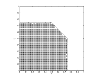
Figure 3: ACPR for a Random Code under ML Decoding

V-B LT Codes

LT codes have been shown to be universal for the single-user erasure channel. Here, we study the performance of LT codes for the two-user erasure channel and consider the case of encoding and decoding at the extremal symmetric point of the Slepian-Wolf region. An LT code is optimized for this point (LT Code I), using linear programming (see Section IV-B), resulting in the degree distribution given by

$$\begin{split}\rho(x)=\;&0.0001+0.0754\cdot x+0.0295\cdot x^{2}+0.0620\cdot x^{3}+\\ &0.0857\cdot x^{7}+0.0718\cdot x^{15}+0.0970\cdot x^{31}+\\ &0.0114\cdot x^{63}+0.5671\cdot x^{127}.\end{split}$$

The performance of this code under iterative decoding is shown in Fig. 4(a). Also shown in Fig. 4(a) is the simulated density evolution threshold for LT code I. The density evolution threshold at the extremal symmetric point is away from capacity for this code due to limiting the maximum check degree in the design process. Also, note that the density evolution threshold is far away from capacity at the corner points of the capacity region. On the other hand, as seen in Fig. 4(b), the code performs much better under ML decoding and is closer to capacity at the corner points of the capacity region. This reinforces the conclusion that most of the sub-universality is due to the iterative decoder, rather than the stability of the code.

In order to achieve capacity at the corner points of the capacity region, LT code II was designed by adding constraints corresponding to the channel conditions at a corner point of the capacity region (see Section IV-B), resulting in the following degree distribution,

$$\begin{split}\rho(x)=\;&0.0001+0.0640\cdot x+0.0251\cdot x^{2}+0.0526\cdot x^{3}+\\ &0.0725\cdot x^{7}+0.0619\cdot x^{15}+0.0806\cdot x^{31}+\\ &0.0082\cdot x^{63}+0.6351\cdot x^{127}.\end{split}$$

The performance of this code under iterative decoding (and the simulated density evolution threshold) ML decoding is shown in Fig. 5(a) and Fig. 5(b) respectively. Note that the density evolution threshold increases only marginally, and the performance under ML decoding is almost the same.

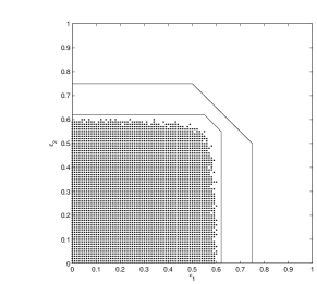
(a) ACPR for LT Code I under Iterative Decoding

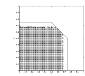
(b) ACPR for LT Code I under ML Decoding

Figure 4: Performance of LT Code I

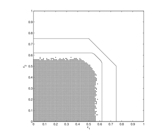
(a) ACPR for LT Code II under Iterative Decoding

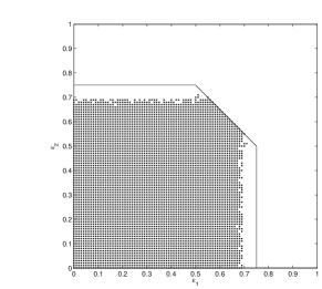
(b) ACPR for LT Code II under ML Decoding

Figure 5: Performance of LT Code II

V-C LDPC Codes

Here, we consider the performance of a punctured $(4,6)$ LDPC code for the joint source-channel coding problem. Two systematic codes were chosen from the ensemble LDPC$(4,6)$, and the systematic bits are punctured before transmission, resulting in a code of rate $1/2$ (two encoded bits are transmitted per source bit).

The $(4,6)$ codes achieve the entire capacity region under ML decoding, as shown in Fig. 6(a), and the iterative decoding threshold is significantly lower as seen in Fig. 6(b). Again, this shows that the iterative decoder is the main reason for the loss of universality.

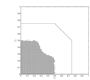
(a) ACPR for a $(4,6)$ LDPC Code under Iterative Decoding

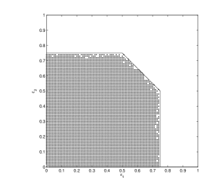
(b) ACPR for a $(4,6)$ LDPC Code under ML Decoding

Figure 6: Performance of $(4,6)$ LDPC Codes

VI Conclusions and Future Work

In this paper, we considered the performance of graph based codes with iterative decoding for obtaining universal performance when transmitting correlated sources over binary erasure channels. We designed an LT code which can achieve the extremal symmetric point. We then showed that an LT code optimized for the symmetric sum-rate point cannot achieve a corner point of the capacity region and, hence, we concluded that LT codes cannot be universal for this two user Slepian-Wolf problem. Our simulation results indicate that a punctured LDPC code ensemble and LT ensemble are nearly universal with maximum likelihood decoding.

For future work, we plan to do the following.

• Analyze the performance of a carefully designed protograph code to try and achieve universality with iterative decoding.

• Since ML decoding is nearly universal and iterative decoding is not universal, we would like to see if there is an enhancement to iterative decoding that can be nearly universal but is yet significantly less complex than ML decoding.

Appendix A Proof of Theorem IV.1

We will use the following Lemma to show that the density evolution equations converge to zero at the extremal symmetric point.

Lemma A.1

$$\rho^{N}(x)>\frac{\mu+\rho(x)}{\mu+G_{N}(p)+1},\text{ for }0\leq x<1-\frac{1}{N}.$$

Proof:

For $0\leq x<1-\frac{1}{N}$, we have

$$\rho^{N}(x) =\frac{\mu+\sum_{i=1}^{N}\frac{\sum_{k=0}^{i-1}\binom{2i-1}{k}p^{k}}{i(1+p)^{2i-1}}x^{i}+x^{N}}{\mu+G_{N}(p)+1}$$

$$=\frac{\mu+\rho(x)+x^{N}}{\mu+G_{N}(p)+1}-$$

$$\phantom{=-}\frac{\sum_{i=N+1}^{\infty}\frac{\sum_{k=0}^{i-1}\binom{2i-1}{k}p^{k}}{i(1+p)^{2i-1}}x^{i}}{\mu+G_{N}(p)+1}$$

$$>\frac{\mu+\rho(x)}{\mu+G_{N}(p)+1}$$

The last step follows from the fact that

$$\sum_{i=N+1}^{\infty}\frac{\sum_{k=0}^{i-1}\binom{2i-1}{k}p^{k}}{i(1+p)^{2i-1}}x^{i} <\sum_{i=N+1}^{\infty}\frac{x^{i}}{i}$$

$$<\frac{1}{N+1}\sum_{i=N+1}^{\infty}x^{i}$$

$$=\frac{1}{N+1}\cdot\frac{x^{N+1}}{1-x}$$

$$<x^{N},$$

where the last step follows from explicit calculations, taking into account that $0\leq x<1-\frac{1}{N}$. ∎

From (IV-C), the convergence criteria for the density evolution equation is given by

$$\begin{split}x>\left[(1-p)+p\bar{\lambda}^{N}(\epsilon,x)\right]\bar{\lambda}^{N}(\epsilon,x)\end{split}$$

Consider the term $\bar{\lambda}^{N}(\epsilon,x)=\lambda\left(1-(1-\epsilon)\rho^{N}(1-x)\right)$. We have,

$$\begin{split}\bar{\lambda}^{N}(\epsilon,x)&=e^{-\alpha(1-\epsilon)\cdot\rho^{N}(1-x)}\\ &\leq e^{-\alpha(1-\epsilon)\frac{\mu+\rho(1-x)}{\mu+G_{N}(p)+1}},\textnormal{ if }x\geq\frac{1}{N}\\ &<e^{-\mu}\cdot\frac{\sqrt{(1-p)^{2}+4px}-(1-p)}{2p}\\ &<\frac{\sqrt{(1-p)^{2}+4px}-(1-p)}{2p},\end{split}$$

where the first inequality follows from Lemma A.1. The polynomial $f(y)=py^{2}+(1-p)y-x$ is a convex function of $y$, with the only positive root at $y=\frac{\sqrt{(1-p)^{2}+4px}-(1-p)}{2p}$. So, if $y<\frac{\sqrt{(1-p)^{2}+4px}-(1-p)}{2p}$, then $f(y)<0$. Hence, $\left[(1-p)+p\bar{\lambda}(\epsilon,x)\right]\bar{\lambda}(\epsilon,x)-x<0$ and the density evolution equation converges, as long as $x\geq\frac{1}{N}$. So, the probability of erasure is upper bounded by $1/N$.

The rate of the code is computed as

$$R=\frac{\int_{0}^{1}\lambda(x)\,\text{d}x}{\int_{0}^{1}\rho^{(N)}(x)\,\text{d}x}.$$

We have

$$\int_{0}^{1}\rho^{N}(x)\,\text{d}x =\frac{\mu+\sum_{i=1}^{N}\frac{\sum_{k=0}^{i-1}\binom{2i-1}{k}p^{k}}{i(i+1)(1+p)^{2i-1}}x^{i}+\frac{1}{N+1}}{\mu+G_{N}(p)+1}$$

also

$$\lim_{N\to\infty}\int_{0}^{1}\rho^{N}(x)\,\text{d}x =\int_{0}^{1}\rho(x)\,\text{d}x$$

$$=1-\frac{p}{2}$$

Note that $\int_{0}^{1}\rho^{(N)}(x)\,\text{d}x$ is a monotonically increasing sequence, upper bounded by $1-\frac{p}{2}$. So, in the limit of infinite blocklengths the design rate is given by

$$R=\frac{(1-\epsilon)(1-e^{-\alpha})}{\mu+(1-\frac{p}{2})}.$$

Appendix B Proof of Theorem IV.2

To analyze the convergence of the ensemble LDGM$\left(n,\lambda(x),\rho^{(N)}(x)\right)$, consider the functions

$$\begin{split}f(x,y)=\left[(1-p)+p\bar{\lambda}^{N}(\epsilon_{2},y)\right]\bar{\lambda}^{N}(\epsilon_{1},x)-x\\ g(x,y)=\left[(1-p)+p\bar{\lambda}^{N}(\epsilon_{1},x)\right]\bar{\lambda}^{N}(\epsilon_{2},y)-y.\end{split}$$

The condition for convergence of the density evolution equations are given by $f(x,y)<0$ and $g(x,y)<0$. When $\epsilon_{1}<\epsilon_{2}$, we can approximately characterize the convergence by analyzing the condition $g(0,y)<0$. We have

$$g(0,y) =\left[(1-p)+p\lambda(\epsilon_{1})\right]\lambda\left(1-(1-\epsilon_{2})\rho^{N}(1-y)\right)-y$$

$$<\left[(1-p)+p\lambda(\epsilon_{1})\right]\lambda\left(1-(1-\epsilon_{2})\rho(1-y)\right)-y$$

$$=k\left(\sqrt{1+ay}-1\right)^{\beta}-y,$$

where

$$k =\left(\frac{\textnormal{e}^{-\mu}(1-p)}{2p}\right)^{\frac{1-\epsilon_{2}}{1-\epsilon_{0}}}\left[(1-p)+p\textnormal{e}^{-\alpha(1-\epsilon_{1})}\right],$$

$$\beta =\frac{1-\epsilon_{2}}{1-\epsilon_{0}}\text{ and }a=\frac{4p}{(1-p)^{2}}$$

The fixed point of $g(0,y)$ can be found by solving

$$y =k\left(\sqrt{1+ay}-1\right)^{\beta},\text{ i.e.,}$$

$$\sqrt{1+ay} =1+k^{-1/\beta}y^{1/\beta}$$

This equation is of the form

$$k^{-2/\beta}y^{(2/\beta-1)} +2k^{-1/\beta}y^{(1/\beta-1)}-a=0,$$

the root of which is approximately equal to the root of the quadratic

$$k^{-2/\beta}z^{2} +2k^{-1/\beta}z-a,$$

where $z=y^{(1/\beta-1/2)}$. The positive root of the quadratic is given by $z=\frac{-1+\sqrt{1+a}}{k^{-1/\beta}}$. So, the fixed point of density evolution is $y\approx\left(\frac{2p}{(1-p)k^{-1/\beta}}\right)^{\frac{2\beta}{2-\beta}}=\left(\frac{2p}{(1-p)k^{-1/\beta}}\right)^{2(1-p)}=\left(\textnormal{e}^{-\mu}\left[(1-p)+p\textnormal{e}^{-\alpha(1-\epsilon_{1})}\right]\right)^{2(1-p)}>0$.

Due to the presence of a constant fixed point, which does not approach $0$ even in the limit of infinite maximum degree, the residual erasure rate is always bounded away from $0$. So, the ensemble LDGM$\left(n,\lambda(x),\rho^{(N)}(x)\right)$ cannot converge at a corner point of the capacity region.

References

- [1] D. Slepian and J. Wolf, “Noiseless coding of correlated information sources,” IEEE Transactions on Information Theory, vol. 19, no. 4, pp. 471–480, 1973.
- [2] J. Garcia-Frias, “Joint source-channel decoding of correlated sources over noisychannels,” in Data Compression Conference, 2001. Proceedings. DCC 2001., 2001, pp. 283–292.
- [3] W. Zhong and J. Garcia-Frias, “LDGM codes for channel coding and joint source-channel coding of correlated sources,” EURASIP Journal on Applied Signal Processing, vol. 2005, no. 6, pp. 942–953, 2005.
- [4] A. Liveris, Z. Xiong, and C. Georghiades, “Joint source-channel coding of binary sources with side information at the decoder using IRA codes,” in 2002 IEEE Workshop on Multimedia Signal Processing, 2002, pp. 53–56.
- [5] ——, “Compression of binary sources with side information at the decoder using LDPC codes,” Communications Letters, IEEE, vol. 6, no. 10, pp. 440–442, Oct 2002.
- [6] M. Luby, “LT codes,” Washington, D.C., Jun. 2002, p. 271.
- [7] T. J. Richardson and R. L. Urbanke, Modern Coding Theory. Cambridge, 2008.