Pointer basis induced by collisional decoherence

Abstract

We study the emergence and dynamics of pointer states in the motion of a quantum test particle affected by collisional decoherence. These environmentally distinguished states are shown to be exponentially localized solitonic wave functions which evolve according to the classical equations of motion. We explain their formation using the orthogonal unraveling of the master equation, and we demonstrate that the statistical weights of the arising mixture are given by projections of the initial state onto the pointer basis.

published in: J. Phys. A: Math. Theor. 43, 015303 (2010)

1 Introduction

The influence of environmental degrees of freedom has been identified as the key concept in explaining the classical behavior of macroscopic systems in a quantum framework [1, 2, 3]. According to this notion a preferred set of localized system states – called the pointer basis [4] – is induced in the course of the interaction of the system with its surrounding. Most characteristically, any initial superposition of these pointer states gets rapidly mixed, while the only states who retain their purity for a long time are the pointer states themselves. While the basic ideas behind the decoherence process seems to be settled, it still remains an open problem to understand the emergence, the dynamics, and the main properties of the pointer states for microscopic realistic environments.

Several strategies have been proposed so far for determining the pointer basis given the environmental coupling. In [5] the suggestion was made to sort all pure states in the Hilbert space according to their linear entropy production rate. The pointer states are then identified with the states having minimal loss of purity. Similar results are obtained by the approach of [6, 7, 8] which is based on a time evolution equation whose solitonic solutions are identified with the pointer states. So far, this concept has been applied to the damped harmonic oscillator [7, 8] and to a free quantum particle coupled linearly to a bath of harmonic oscillators [6, 8]. There, the solitonic solutions of the corresponding nonlinear equation are coherent states and Gaussian wave packets, respectively. Moreover, the decoherence to Gaussian pointer states was proved to be generic for linear coupling models [9].

In this paper, we extend the analysis from linear models to a non-perturbative treatment of the interaction. We focus on the model of collisional decoherence, which provides a realistic description of the decoherence process generated by an ideal gas environment. Notably, experiments with interfering fullerene molecules displayed a reduction of interference visibility in agreement with this model [10, 11, 12, 13, 14]. We derive the corresponding pointer states which are shown to form an overcomplete, exponentially localized set of basis states, and we prove decoherence to these states using the orthogonal unraveling of the master equation [15, 16]. This stochastic process on the one hand provides the statistical weights of the pointer basis, and on the other hand represents an efficient way of solving master equations which exhibit pointer states. Moreover, it explains the emergence of classical Hamiltonian dynamics.

The main result was already announced in [17]. Here, we provide a more detailed explanation of the proofs and derivations. As an extension of [17], we prove the decoherence dynamics for a more general situation where the localization rate of collisional decoherence is in a non-saturated regime, and we utilize the relative entropy in order to illustrate the emergence of the statistical weights.

While the above results are derived within the framework of decoherence theory, they can also be applied to dynamic reduction models which propose a modification of the Schrödinger equation by means of nonlinear and stochastic terms. In fact, the observational consequences of the Ghirardi-Rimini-Weber (GRW) spontaneous localization model [18, 19] are equivalent to the ones of collisional decoherence, since they are described by the same master equation [20]. The present work therefore applies to the GRW model. In particular, it provides the corresponding pointer basis.

The structure of the article is as follows. In Sect. 2, we briefly review the notion of pointer states, and we summarize the method for determining the pointer states discussed in [7, 6, 8]. In order to motivate the approach, we consider a two level system and a dephasing process. This method is then applied to collisional decoherence in Sect. 3, which provides a set of solitonic states to be regarded as ‘candidate’ pointer states. We show in Sect. 4 that these solitons form an overcomplete basis of exponentially localized states, and we give an expression for their spatial extension. Moreover, we demonstrate that the ‘candidate’ pointer states move on classical phase space trajectories if they are sufficiently localized. In Sect. 5, we briefly review the method of quantum trajectories, focusing in particular on the orthogonal unraveling of the master equation. This stochastic process is then applied to collisional decoherence which allows us to show that the ‘candidate’ states are indeed pointer states in the sense of the definition given in Sect. 2. Furthermore, we use the orthogonal unraveling to show that the statistical weights of the pointer states are given by the overlap with the initial state. We present our conclusion in Section 6.

2 The pointer basis

2.1 Definition of pointer states

To motivate the definition of pointer states, let us consider the quantum dynamics of the damped harmonic oscillator. Its evolution can be described by a master equation in Lindblad form defined by the standard Hamiltonian $\mathsf{H}=\hbar w\mathsf{a}^{{\dagger}}\mathsf{a}$, and a single Lindblad operator $\mathsf{L}=\mathsf{a}$, with associated rate $\gamma$ [21]. We take as initial state a superposition of two quasi-orthogonal coherent states

$$|\psi_{0}\rangle = c_{1}|\alpha_{0}\rangle+c_{2}|\beta_{0}\rangle\,,\hskip 20.00003pt{\rm with}\,\,\left|\alpha_{0}-\beta_{0}\right|^{2}\gg 1\,,$$ (1)

which satisfy $\mathsf{a}|\alpha\rangle=\alpha|\alpha\rangle$, with $\alpha\in\mathbbm{C}$. It is then easy to show that for times larger than the decoherence time $t_{{\rm dec}}=2\left|\alpha_{0}-\beta_{0}\right|^{-2}/\gamma$ the solution of the master equation is well approximated by [22, 21]

$$\rho_{t} \simeq \left|c_{1}\right|^{2}|\alpha_{t}\rangle\langle\alpha_{t}|+\left|c_{2}\right|^{2}|\beta_{t}\rangle\langle\beta_{t}|\,,\hskip 20.00003pt{\rm if}\,\,t\gg t_{{\rm dec}}\,,$$ (2)

with $\alpha_{t}=\alpha_{0}\,\exp\left(-iwt-\gamma t/2\right)$. Thus, any coherent state remains pure during the damped time evolution, while any superposition of distinct coherent states decays into a mixture (with a decay rate $\gamma_{{\rm dec}}=1/t_{{\rm dec}}\gg\gamma$) whose statistical weights are determined by the initial overlaps $\left|\langle\alpha_{0}|\psi_{0}\rangle\right|^{2}$ and $\left|\langle\beta_{0}|\psi_{0}\rangle\right|^{2}$. Due to this property, the coherent states are to be identified with the pointer states of the damped harmonic oscillator.

The above observation serves as the starting point for the following definition of the pointer states for an open quantum system evolving according to a Lindblad master equation $\partial_{t}\rho=\mathcal{L}\rho$. One says that the system exhibits a pointer basis if its dynamics involves a separation of time scales, characterized by a fast decoherence time $t_{{\rm dec}}$, such that for any time much larger than $t_{{\rm dec}}$, the evolved state is well approximated by a mixture of uniquely defined pure states $\mathsf{P}_{\alpha}=|\pi_{\alpha}\rangle\langle\pi_{\alpha}|$ which are independent of the initial state $\rho_{0}$,

$$e^{\mathcal{L}t}\rho_{0} \simeq \int\mathrm{d}\alpha\,\,{\rm Prob}\left(\alpha|\rho_{0}\right)\mathsf{P}_{\alpha}(t),\hskip 20.00003pt{\rm if}\,\,\mbox{\rm$t\gg t_{{\rm dec}}$}\,,$$ (3)

with ${\rm Prob}\left(\alpha|\rho_{0}\right)\geqslant 0,\int\mathrm{d}\alpha\,{\rm Prob}\left(\alpha|\rho_{0}\right)=1$. Following the above example, we further demand that for initial states $\rho_{0}$, which are superpositions of mutually orthogonal pointer states $\mathsf{P}_{\beta}$, the probability distribution ${\rm Prob}\left(\alpha|\rho_{0}\right)=\sum_{\beta}w_{\beta}\delta\left(\alpha-\beta\right)$ is given by the initial projections

$$w_{\beta} = {\rm Tr}\left(\rho_{0}\mathsf{P}_{\beta}\left(0\right)\right)\,.$$ (4)

The pointer states $\mathsf{P}_{\alpha}$ initially form an (overcomplete) basis, and they may evolve in time, though slowly compared to $t_{{\rm dec}}$.

The name pointer state was coined in [4] due to its relevance for the physical description of a measurement apparatus. A measurement device which probes an observable $\mathsf{A}$ is constructed such that macroscopically distinct positions of the pointer or indicator are obtained for the different eigenstates of $\mathsf{A}$. For a quantum system initially prepared in an eigenstate of $\mathsf{A}$ the read-out will display the corresponding eigenvalue with certainty provided these pointer states remain pure during the time evolution. On the other hand, if the quantum system is prepared in a superposition of eigenstates of $\mathsf{A}$, we expect the pointer not to end up in a superposition of different read-out states, but rather to be at a definite position, though probabilistically, with probabilities given by the overlap (4).

We emphasize that the importance of pointer states goes beyond the physics of measurement devices and the quantum-to-classical transition since they are also a practical tool for the solution of master equations. Knowing the pointer states $\mathsf{P}_{\alpha}$, their time evolution $\mathsf{P}_{\alpha}\left(t\right)$, and their probabilities ${\rm Prob}\left(\alpha|\rho_{0}\right)$, one can immediately specify the solution of the master equation for any initial state and times greater than the decoherence time. Since the decoherence time is generically much shorter than the system and dissipation time scales of the pointer state motion, this allows one to capture a large part of the system evolution without solving the master equation.

2.2 Pointer states of pure dephasing  

A practical way to obtain the pointer states $\mathsf{P}_{\alpha}$, for a given environmental coupling, was discussed in [6, 7, 8]. We will illustrate this method by means of a two level system, suspect to a dephasing environment. The corresponding master equation in interaction picture,

$$\partial_{t}\rho =\, \gamma\left(\sigma_{z}\,\rho\,\sigma_{z}-\rho\right)\,,$$ (5)

is characterized by the Lindblad jump operator $\mathsf{L=}\sigma_{z}\sqrt{\gamma}$ $\left(\gamma>0\right)$. In Bloch representation, $\rho_{t}=1/2\left(\mathsf{I}+\boldsymbol{a}\left(t\right)\cdot\boldsymbol{\sigma}\right)$ with Bloch vector $\boldsymbol{a}\boldsymbol{}\left(t\right)={\rm Tr}\left(\boldsymbol{\sigma}\rho\left(t\right)\right)$ and Pauli matrices $\boldsymbol{\sigma}=\left(\sigma_{x},\sigma_{y},\sigma_{z}\right)$, the solution reads

$$\boldsymbol{a}\boldsymbol{}\left(t\right) = \left(e^{-2\gamma t}a_{x}\left(0\right),e^{-2\gamma t}a_{y}\left(0\right),a_{z}\left(0\right)\right)\,.$$ (6)

Thus, the Bloch sphere $\left\{\boldsymbol{a}:\left|\boldsymbol{a}\right|=1\right\}$, which represents the set of all pure states, is projected onto the z-axis in the course of the dephasing process. This implies that the decohered state $\boldsymbol{a}\left(\infty\right)=\left(0,0,a_{z}\left(0\right)\right)$ is a mixture of the eigenstates of $\sigma_{z}$ (denoted by $\mathsf{P}_{\downarrow}=|\downarrow\rangle\langle\downarrow|$ and $\mathsf{P}_{\uparrow}=|\uparrow\rangle\langle\uparrow|$ respectively),

$$\rho_{\infty} = \,{\rm Tr}\left[\mathsf{P_{\uparrow}}\rho_{0}\right]\mathsf{P_{\uparrow}}+{\rm Tr}\left[\mathsf{P_{\downarrow}}\rho_{0}\right]\mathsf{P_{\downarrow}\,}.$$ (7)

The comparison with (3) shows that the north and the south pole of the Bloch sphere (corresponding to $\mathsf{P}_{\downarrow}$ and $\mathsf{P}_{\uparrow}$) form the pointer basis of the pure dephasing process.

Since the solution of the master equation will not be at hand in general, one requires a method which yields the pointer states without the knowledge of $\rho_{t\,}$. To motivate this, we notice that the north pole of the Bloch sphere is the asymptotic end point of the trajectory illustrated by the thick line in Fig. 1. This trajectory is generated by an equation of motion with the following properties. (i) It is nonlinear because it must distinguish pointer states from their superpositions. (ii) It preserves the purity of pure initial states, i.e. an initial state which lies on the Bloch sphere remains on the surface. (iii) The generated trajectory follows the exact solution of the master equation as close as possible. In order to find such an equation of motion, it is suggestive to minimize the distance of the initial increments, i.e.

$$\min_{\partial_{t}\boldsymbol{a}}|\mathcal{L}\left(\boldsymbol{a}\right)-\partial_{t}\boldsymbol{a}|^{2}\,,\hskip 20.00003pt{\rm with}\;\boldsymbol{a}\cdot\partial_{t}\boldsymbol{a}=0\,.$$ (8)

Here, $\mathcal{L}$ denotes the generator of the master equation (5) in Bloch representation and $\partial_{t}\boldsymbol{a}$ is subject to the condition that the generated trajectory remains on the surface of the Bloch sphere. The solution of the above optimization problem reads, in spherical coordinates,

$$\left(\dot{r},\dot{\varphi},\dot{\theta}\right) = \left(0,0,-\gamma\sin\left(2\theta\right)\right)\,.$$ (9)

Since the sine is positive for $\theta\in\left(0,\pi/2\right)$, the solutions of these equations tend asymptotically towards a pointer state of the system, see Fig. 1. The equator of the Bloch sphere forms a set of unstable fixed points of (9).

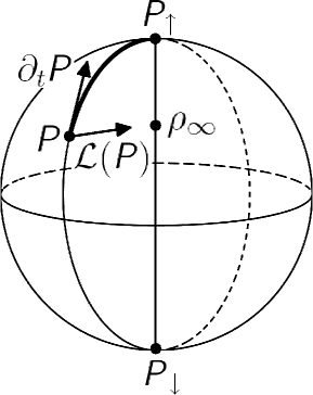
Figure 1: Bloch representation of a two level system subject to pure dephasing, as described by (5). As $t\rightarrow\infty$, the initial state $\rho_{0}=\mathsf{P}$ is projected onto the z-axis, implying that the poles ($\mathsf{P}_{\uparrow}$ and $\mathsf{P}_{\downarrow}\,$) are the pointer states. The thick line indicates a trajectory within the set of pure states which connects the initial state to a nearby pointer state (the north pole). The equation of motion for this trajectory has minimal distance from $\mathcal{L}\left(\mathsf{P}\right)$ among all equations which generate pure state trajectories.  

2.3 Nonlinear equation for pointer states

Let us now generalize the above argument to general Markovian master equations. Replacing the Euclidean norm by the Hilbert-Schmidt norm $\|\cdot\|_{\rm{HS}}$ in the space of operators, the generalization of (8) to higher dimensional systems reads

$$\min_{\mathsf{}\partial_{t}\mathsf{P}}||\mathcal{L}\left(\mathsf{P}\boldsymbol{}\right)-\mathsf{}\partial_{t}\mathsf{P}||_{\rm{HS}}^{2}\,,$$ (10)

where the minimization is with respect to all evolution equations $\mathsf{}\partial_{t}\mathsf{P}=f\left(\mathsf{P}\right)$ which propagate $\mathsf{P}$ within the set of pure states, such that $\mathsf{P}_{t}^{2}=\mathsf{P}_{t}\,$. It can be shown that the general structure of an equation that evolves state vectors $|\psi\rangle$ preserving their normalization has the structure $\partial_{t}|\psi\rangle=\left(\mathsf{A}_{\psi}-\langle\psi|\mathsf{A}_{\psi}|\psi\rangle+\mathsf{B}_{\psi}\right)|\psi\rangle$, with $\psi$-dependent, hermitian and anti-hermitian mappings $\mathsf{A}_{\psi}=\mathsf{A}_{\psi}^{{}^{{\dagger}}}$ and $\mathsf{B}_{\psi}=-\mathsf{B}_{\psi}^{{}^{{\dagger}}}\,$. This implies that the equation of motion for the projector $\mathsf{P}=|\psi\rangle\langle\psi|$ must be of the form $\partial_{t}\mathsf{P}=\left[\mathsf{P},\left[\mathsf{P},\mathsf{X}_{\mathsf{P}}\right]\right]\,,$where $\mathsf{X}_{\mathsf{P}}:=\mathsf{A}_{\mathsf{P}}+\left[\mathsf{B}_{\mathsf{P}},\mathsf{P}\right]$. Using this form, the optimization problem (10) reduces to $\min_{\mathsf{X}}\|\mathcal{L}\left(\mathsf{P}\right)-\left[\mathsf{P},\left[\mathsf{P},\mathsf{X}\right]\right]\|_{\rm{HS}}\,$. As shown in [7] the solution is determined by the generator of the master equation, $\mathsf{X}_{\min}=\mathcal{L}\left(\mathsf{P}\right)$. Hence, the generalization of (9) reads as [6, 7, 8]

$$\partial_{t}\mathsf{P} = \left[\mathsf{P},\left[\mathsf{P},\mathcal{L}\left(\mathsf{P}\right)]]\,.\right.\right.$$ (11)

Motivated by the example in Sect. 2.2, one conjectures that the asymptotic solutions of (11) provide the pointer states in more complex systems as well.

It will be important below that Eq. (11) is known also in another context: it corresponds to the deterministic part of the orthogonal unraveling of the master equation. As we will demonstrate in Section 5, one can use this specific unraveling to prove for a specific model that the asymptotic solutions of (11) indeed provide the pointer states.

3 Pointer states of collisional decoherence

3.1 Collisional decoherence

In order to assess the nonlinear equation (11) in the context of a nontrivial environmental coupling we now apply it to the model of collisional decoherence [23, 24]. The latter describes the motion of a quantum test particle in an ideal gas environment and it accounts for the quantum effects of the scattering dynamics in a non-perturbative fashion. The corresponding master equation has Lindblad form,

$$\partial_{t}\rho = -\frac{i}{\hbar}\left[\mathsf{H},\rho\right]+\int\mathrm{d}q\left(\mathsf{L}_{q}\rho\mathsf{L}^{{}^{{\dagger}}}_{q}-\frac{1}{2}\mathsf{L}^{{}^{{\dagger}}}_{q}\mathsf{L}_{q}\rho-\frac{1}{2}\rho\mathsf{L}^{{}^{{\dagger}}}_{q}\mathsf{L}_{q}\right)\,,$$ (12)

where the jump operators are proportional to momentum kick operators, $\mathsf{L}_{q}=\sqrt{\gamma G\left(q\right)}e^{iq\mathsf{x}}$ (with position operator $\mathsf{x}$). The continuous label $q$ has the meaning of a momentum transfer experienced by the test particle with $G\left(q\right)\geq 0$ the corresponding distribution, $\int\mathrm{d}q\,G\left(q\right)=1$; $\gamma$ is the collision rate of the gas environment. The 1d equation of motion thus reads

$$\partial_{t}\rho = \frac{1}{i\hbar}\left[\mathsf{H},\rho\right]+\gamma\int_{-\infty}^{\infty}\mathrm{d}q\,G\left(q\right)e^{iq\mathsf{x}/\hbar}\rho e^{-iq\mathsf{x}/\hbar}-\gamma\rho\,.$$ (13)

It leads to a localization in position space, i.e. to a loss of spatial coherence, as can be seen by switching to the interaction picture, $\tilde{\rho}=e^{i\mathsf{H}t/\hbar}\rho e^{-i\mathsf{H}t/\hbar}$, and the position representation,

$$\partial_{t}\langle x|\tilde{\rho}|x^{\prime}\rangle = -F\left(x-x^{\prime}\right)\langle x|\tilde{\rho}|x^{\prime}\rangle\,.$$ (14)

The decay rate of the spatial coherences is thus characterized by a localization rate $F\left(s\right)\geq 0$ which is related to the momentum transfer distribution $G\left(q\right)\,$ by

$$F\left(s\right) = \gamma\left(1-\int_{-\infty}^{\infty}\mathrm{d}q\,G\left(q\right)e^{i{\rm qs}/\hbar}\right)\,.$$ (15)

Since the Fourier transform of the distribution $G\left(q\right)$ tends to zero for large distances $s$, the localization rate saturates for large $s$ at the maximum value given by the collision rate, $F\left(s\rightarrow\infty\right)=\gamma\,$, which can be interpreted as the limit where one collision is sufficient to reveal the particles ‘which path’ information. This behavior is in sharp contrast to linear models, where the localization rate grows quadratically, and thus approaches infinity in the limit of a large separation $s$.

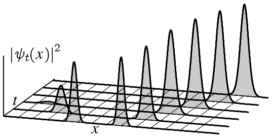
Figure 2: Formation of pointer states: an initial superposition of counter-propagating, localized states is evolved numerically according to the nonlinear equation (19). It forms into a solitonic solution which moves with a fixed shape and constant velocity. These solitons are interpreted as the pointer states of collisional decoherence.

3.2 Determining the pointer states of collisional decoherence

In order to apply the nonlinear equation (11) to collisional decoherence (13) of a free particle, that is $\mathsf{H}=\mathsf{p}^{2}/2m\,$, we rewrite the projector equation (11) in vector representation and choose for $\mathcal{L}$ the Lindblad form (12), which gives [7, 8]

$$\partial_{t}|\psi\rangle = \frac{1}{i\hbar}\left(\mathsf{H}-\langle\mathsf{H}\rangle_{\psi}\right)\mathsf{}|\psi\rangle$$ (16)

$$+\int_{-\infty}^{\infty}\mathrm{d}q\,\left(\langle\mathsf{L}^{{\dagger}}_{q}\rangle_{\psi}\left(\mathsf{L_{q}}-\langle\mathsf{L}_{q}\rangle_{\psi}\right)-\frac{1}{2}\left(\mathsf{\mathsf{L}^{{\dagger}}_{q}}\mathsf{L}_{q}-\langle\mathsf{\mathsf{L}^{{\dagger}}_{q}}\mathsf{L}_{k}\rangle_{\psi}\right)\right)|\psi\rangle\,.$$

The expectation value $\langle\mathsf{H}\rangle_{\psi}$ is disregarded in the following, since it contributes only an additional phase. Now, we choose the jump operator of collisional decoherence, $\mathsf{L}_{q}=\sqrt{\gamma G\left(q\right)}e^{iq\mathsf{x}}$, and switch to position representation, which yields

$$\partial_{t}\psi_{t}\left(x\right) = -\frac{\hbar}{2mi}\partial_{x}^{2}\psi_{t}\left(x\right)+\psi_{t}\left(x\right)\Lambda\left[\left|\psi_{t}\right|^{2}\right]\left(x\right)\,,$$ (17)

$$\Lambda\left[\left|\psi_{t}\right|^{2}\right]\left(x\right) = \gamma\left(|\psi_{t}|^{2}\ast\hat{G}\left(x\right)-\int^{\infty}_{-\infty}\mathrm{d}y|\psi_{t}|^{2}\left(y\right)\left(|\psi_{t}|^{2}\ast\hat{G}\right)\left(y\right)\right)\,.$$ (18)

Here, $g\ast h(x)\equiv\int^{\infty}_{-\infty}\mathrm{d}yg\left(y\right)h\left(x-y\right)$ denotes the convolution and $\hat{G}\left(x\right)$ is the Fourier transform of $G\left(q\right)\,$, i.e. $\hat{G}\left(x\right)\equiv\int_{-\infty}^{\infty}\mathrm{d}q\,G\left(q\right)\exp\left(iqx/\hbar\right)\,$.

The two summands in (17) have counteractive effects on the temporal evolution of the wave function: the coherent term leads to its dispersion, whereas the second, incoherent summand tends to localize the solution. In order to explain this localization, we note that the second summand in (18) is independent of $x$. This implies that the centered parts of the wave function, where the convolution $|\psi_{t}|^{2}\ast\hat{G}\left(x\right)$ exceeds the constant term in (18), get amplified, i.e. $\partial_{t}\psi_{t}>0$, whereas the tails of the wave function get damped, i.e. $\partial_{t}\psi_{t}<0$. As a consequence of these competing effects, solutions of (17) evolve towards solitonic states where both effects are in equilibrium, such that the state moves with fixed shape and constant velocity. As discussed above, these solitons are candidates for the pointer states of collisional decoherence.

Assuming the momentum transfer distribution $G\left(q\right)$ to be a centered Gaussian with variance $\sigma_{G}^{2}\,$, we can rewrite (17) in dimensionless form.

$$\partial_{\tau}\varphi_{\tau}\left(y\right) = -\frac{\kappa}{2i}\partial_{y}^{2}\varphi_{\tau}\left(y\right)+\varphi_{\tau}\left(y\right)\int_{-\infty}^{\infty}\mathrm{d}y^{\prime}|\varphi_{\tau}\left(y^{\prime}\right)|^{2}$$ (19)

$$\times\left(e^{-\left(y-y^{\prime}\right)^{2}/2}-\int^{\infty}_{-\infty}\mathrm{d}y^{\prime\prime}|\varphi_{\tau}\left(y^{\prime\prime}\right)|^{2}e^{-\left(y^{\prime}-y^{\prime\prime}\right)^{2}/2}\right)$$

Here we use the dimensionless variables $y\equiv\sigma_{G}x/\hbar\,$ and $\tau\equiv\gamma t\,$ to define the dimensionless wave function $\varphi_{\tau}\left(y\right)\equiv\sqrt{\hbar/\sigma_{G}}\psi_{\tau/\gamma}\left(\hbar y/\sigma_{G}\right)\,$. Notably, Eq. (19) depends only on the single dimensionless parameter $\kappa\equiv\sigma_{G}^{2}/\left(m\hbar\gamma\right)\,$.

Figure 2 shows a numerical solution of (19), where we choose a superposition of two counter propagating localized states $\phi_{1,2}$ as the initial state, $\psi_{0}\left(x\right)=c_{1}\phi_{1}\left(x\right)+c_{2}\phi_{2}\left(x\right)$. As expected from the above discussion, the (modulus of the) solution converges to a soliton. Moreover, we find that the soliton inherits its initial position and momentum expectation value from that localized component $\phi_{i}$ of the initial state which has the greatest weight $c_{i}$, $\left|c_{i}\right|>\left|c_{j\neq i}\right|$. Similar observations are found for various other initial states.

4 Properties of the soliton basis

We proceed to characterize the solitonic solutions of (17). In Sect. 4.1, the consequences of the conservation of probability on the phase of the solitons are analyzed, allowing us to predict the asymptotic shape of the solitons in Sect. 4.2. In Sect. 4.3 we estimate the spatial extension of the solitons, followed by the proof that they form a basis of the Hilbert space in Sect. 4.4. Finally, in Sect. 4.5, we discuss the dynamics of the solitonic solutions in the presence of an external potential.

4.1 Consequences of the continuity equation

As demonstrated in the previous section, the nonlinear equation (17) exhibits solitonic solutions $\pi_{t}\left(x\right)$ in the sense that the modulus of $\pi_{t}\left(x\right)$ moves with constants shape and velocity, i.e.

$$\pi_{t}\left(x\right) = f\left(x-vt\right)e^{ig\left(x,t\right)}\,,$$ (20)

with $f\geqslant 0$ and $g$ real. In this section, we analyze the general structure of the phase $g\left(x,t\right)$, which will be relevant subsequently. The time derivative of a solution $\left|\psi_{t}\left(x\right)\right|^{2}$ of (17), yields the continuity equation for $\psi_{t}\left(x\right)$,

$$\partial_{t}\mbox{\rm$\left|\psi_{t}\left(x\right)\right|^{2}\,$ } = -\frac{\hbar}{m}\partial_{x}{\rm Im}\left(\psi_{t}^{\ast}\partial_{x}\psi_{t}\right)+2\mbox{\rm$\left|\psi_{t}\left(x\right)\right|^{2}\,$}\Lambda\left[|\psi_{t}|^{2}\right]\left(x\right)\,.$$ (21)

Plugging the solitonic solution (20) into (21), gives

$$-2\Lambda\left[f^{2}\right]\left(x-vt\right)-v\partial_{x}\log f^{2}\left(x-vt\right) = -\frac{\hbar}{m}(\partial_{x}^{2}g\left(x,t\right)$$ (22)

$$\left.+\partial_{x}g\left(x,t\right)\partial_{x}\log f^{2}\left(x-vt\right)\right)\,.$$

Here we have used that $\Lambda\left[f_{t}^{2}\right]\left(x\right)=\Lambda\left[f^{2}\right]\left(x-vt\right)$, which follows from $f_{t}\left(x\right)=f\left(x-vt\right)$ . The time dependence of the left hand side of (22) corresponds to a spatial shift. Thus, also the right hand side of (22) must exhibit such a simple time dependence, which implies that

$$-v\partial_{x}r\left(x,t\right)\, = \partial_{t}r\left(x,t\right)\,,$$ (23)

where $r\left(x,t\right)$ denotes the right hand side of (22). It follows that

$$-v\partial_{x}^{3}g\left(x,t\right)-v\partial_{x}^{2}g\left(x,t\right)\partial_{x}\log f^{2}\left(x-vt\right) = \partial_{t}\partial^{2}_{x}g\left(x,t\right)$$ (24)

$$+\partial_{t}\partial_{x}g\left(x,t\right)\partial_{x}\log f^{2}\left(x-vt\right)\,.$$

Since this equation must hold for all $x,v$ and $t$, we may assume that the equality holds already for the summands, such that

$$-v\partial_{x}^{2}g\left(x,t\right) = \partial_{t}\left[\partial_{x}g\left(x,t\right)\right]\,.$$ (25)

Therefore, the temporal and spatial dependence of the phase has the general structure

$$g\left(x,t\right) = \phi\left(x-vt\right)+\chi\left(t\right)\,,$$ (26)

with unknown functions $\phi$ and $\chi$.

4.2 Asymptotic form of the solitons

To explore the tails of the solitonic states $\pi_{t}\left(x\right)$ let us consider the form of (17) for asymptotically large positions. It reads

$$\partial_{t}\psi_{t}\left(x\right) \sim -\frac{\hbar}{2mi}\partial_{x}^{2}\psi_{t}\left(x\right)-\gamma a_{\psi}\psi_{t}\left(x\right)\,,\hskip 20.00003pt{\rm for}\,\,\left|x\right|\rightarrow\infty\,,$$ (27)

with $a_{\psi}\equiv\int^{\infty}_{-\infty}\mathrm{d}y|\psi_{t}|^{2}\left(y\right)\left(|\psi_{t}|^{2}\ast\hat{G}\right)\left(y\right)$ a $\psi$-dependent, positive constant. Inserting the solitonic form (20) into (27) yields

$$i\partial_{t}g\left(x,t\right)f\left(x-vt\right) = i\frac{\hbar}{2m}\left[\partial_{x}^{2}f\left(x-vt\right)-f\left(x-vt\right)\left(\partial_{x}g\left(x,t\right)\right)^{2}\right]+vf\left(x-vt\right)$$ (28)

$$-\frac{\hbar}{m}\left[\partial_{x}f\left(x-vt\right)\partial_{x}g\left(x,t\right)+f\left(x-vt\right)\partial_{x}^{2}g\left(x,t\right)\right]$$

$$-\gamma a_{\psi}f\left(x-vt\right)\,.$$

Using (26), we find that both $\partial_{x}g\left(x,t\right)$ and $\partial_{x}^{2}g\left(x,t\right)$ are only a function of $x_{t}=x-vt$, and accordingly, that also the left hand side of (28) must be a function of $x_{t}$. If follows that $\chi\left(t\right)$ is at most linear in $t\,$ (that is $\chi\left(t\right)=\chi_{1}t+\chi_{0}\,$, with unknown constants $\chi_{0}$ and $\chi_{1}$). Considering the real and imaginary part of (28) separately, one obtains two coupled (second order) differential equations

$$v\partial_{x}f-\gamma a_{\psi}f = \frac{\hbar}{m}\left(\partial_{x}f\partial_{x}\phi+\frac{1}{2}f\partial_{x}^{2}\phi\right)\,,$$ (29)

$$\left(\chi_{1}-v\partial_{x}\phi\right)f = \frac{\hbar}{2m}\left(\partial_{x}^{2}f-f\left[\partial_{x}\phi\right]^{2}\right)\,,$$ (30)

where $f\equiv f\left(x-vt\right)$ and $\phi\equiv\phi\left(x-vt\right)$. This set of equations has two unique solutions

$$f\left(x\right) = e^{\pm k\left|x\right|}\,,$$ (31)

$$\phi\left(x\right) = \mp{\rm sgn}\left(x\right)\frac{m}{\hbar}\left(v+\frac{\gamma a_{\psi}}{k}\right)x,$$ (32)

where the constant $k>0$ depends on the boundary condition for (29) (which can be determined only by solving the full nonlinear equation (17)). The solution with the positive exponent in (31) is irrelevant, since it is not normalizable. Figure 3 confirms that the tails of the numerically obtained solitonic solutions of (19) are in agreement with the functional form (31); they are straight lines in the semi-logarithmic plot. This shows that, unlike in linear models [25] where the pointer states are Gaussian, the pointer states of collisional decoherence are exponentially localized.

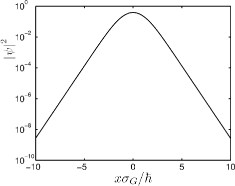
Figure 3: Semi-logarithmic plot of the numerical solitonic solution of (19). The graph clearly demonstrates that the pointer states have exponential tails.

4.3 Size of the solitons

An important characteristic of the pointer states is their spatial extension. As explained in [17], the latter can be related to the experimentally accessible one-particle coherence length of a thermal gas. We will determine the pointer width in this section, and apply the result later, when studying the dynamics of pointer states in an external potential.

As a first step, consider the standard deviation $\tilde{\sigma}_{\pi}$ of the numerically obtained dimensionless solitonic solution $\left|\tilde{\pi}\left(y\right)\right|^{2}$ of (19) as a function the dimensionless parameter $\kappa=\sigma_{G}^{2}/\left(\gamma m\hbar\right)\,$. As shown by the solid line in Fig. 4, the size $\tilde{\sigma}_{\pi}$ increases linearly with $\kappa\,$.

This observation can be reproduced by a simplified model which has the practical advantage that it can be applied to more complex systems, such as 3D gases with a microscopically realistic localization rate $F\,$ [17]. The idea of the model goes as follows: the ideal gas environment consists of particles which collide with the system at a rate $\gamma$. At each collision, the ambient particles gain position information, such that the wave function gets spatially localized to a length scale $\ell_{{\rm loc}}\,$ determined by the localization rate $F$, see (14). After the scattering event, the particle disperses freely, until it gets localized again by a subsequent collision. The pointer width $\sigma_{\pi}$ is then obtained by averaging the time-dependent width of the wave function over the waiting time distribution of a Poisson process.

More specifically, we assume that the length scale $\ell_{{\rm loc}}$ is characterized by the free parameter

$$a_{{\rm loc}}^{\prime} = \frac{F\left(\ell_{{\rm loc}}\right)}{F\left(\infty\right)}\,.$$ (33)

Using (15) and taking the momentum transfer distribution $G\left(q\right)$ to be a centered Gaussian with variance $\sigma_{G\,}^{2}$, we obtain

$$\ell_{{\rm loc}} = \frac{a_{{\rm loc}}\,\hbar}{\sigma_{G}}\>,$$ (34)

with $a^{2}_{{\rm loc}}=-2\log\left(1-a_{{\rm loc}}^{\prime}\right)$. The free dispersion after the collision yields the time dependent size

$$\sigma^{2}_{\pi}\left(t\right) = \ell_{{\rm loc}}^{2}+\left(\frac{\hbar t}{2m\ell_{{\rm loc}}}\right)^{2}\,.$$ (35)

Finally, the average over the waiting time distribution ${\rm Prob}\left(t\right)=\gamma e^{-\gamma t}$ gives

$$\sigma_{\pi} \equiv \int_{0}^{\infty}\mathrm{d}\tau{\rm Prob}\left(\tau\right)\frac{1}{\tau}\int_{0}^{\tau}\mathrm{d}t\sigma_{\pi}\left(t\right)$$ (36)

$$\simeq a_{{\rm loc}}\frac{\hbar}{\sigma_{G}}+\frac{\sigma_{G}}{4a_{{\rm loc}}m\gamma}\,,$$

where we use a linearization of $\sigma_{\pi}\left(t\right)$ in the second line. The dimensionless version of (36) reads

$$\tilde{\sigma}_{\pi} \equiv \frac{\sigma_{\pi}\sigma_{G}}{\hbar}$$ (37)

$$= a_{{\rm loc}}+\frac{1}{4a_{{\rm loc}}}\kappa\,.$$

The dashed line in Figure 4 shows that the form of this equation agrees with the numerical solution of (19); the fit yields a value of $a_{{\rm loc}}\simeq 0.4$ for the parameter characterizing the localization length scale.

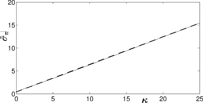
Figure 4: Spatial extension of the solitonic solution of (19) as a function of the dimensionless parameter $\kappa=\sigma_{G}^{2}/\left(\gamma m\hbar\right)$. The solid line represents the numerical solution of (19). The result of the localization model (37) with parameter $a_{{\rm loc}}=0.4$ is given by the dashed line.

4.4 Completeness of the soliton basis

Our next aim is to show that the solitonic solutions of (17), which are interpreted below as the pointer states of collisional decoherence, form an overcomplete basis. For this purpose, we first present a general method to construct a whole manifold of solutions of (11) given a specific one. It relies on the symmetry properties of the corresponding master equation. Since collisional decoherence exhibits Galilean (i.e. translation and boost) invariance, it is then easy to show that the pointer states of this model form an overcomplete basis.

Suppose there is a family of unitary operators $\mathsf{U_{t}}$, satisfying

$$\hskip 10.00002pt\mathsf{\mathsf{U}_{t}}\,\mathcal{D}\left(\rho\right)\,\mathsf{U}_{t}^{{}^{{\dagger}}} = \mathcal{D}\left(\mathsf{\mathsf{U}_{t}}\,\rho\,\mathsf{U}_{t}^{{}^{{\dagger}}}\right),$$ (38)

$$\hskip 40.00006pt\partial_{t}\,\mathsf{\mathsf{U}_{t}} = \frac{1}{i\hbar}\left[\mathsf{H},\mathsf{\mathsf{U}_{t}}\right],$$ (39)

where we denote by $\mathcal{D}$ the incoherent part of the master equation, $\mathcal{L}\left(\rho\right)\equiv\left[\mathsf{\mathsf{H}},\rho\right]/\left(i\hbar\right)+\mathcal{D}\left(\rho\right)$. Then, given a solution $P_{t}$ of the nonlinear equation (11), also $\mathsf{\mathsf{\mathsf{\mathsf{U}_{t}}\mathsf{P_{t}}}\,\mathsf{U}_{t}^{{}^{{\dagger}}}}$ constitutes a solution of (11).

This can be verified easily:

$$\left[\mbox{\rm$\mathsf{U}\mathsf{P}\mathsf{U}^{{\dagger}}$},\left[\mathsf{U}\mathsf{P}\mathsf{U}^{{\dagger}},\mathcal{L}\left(\mbox{\rm$\mathsf{U}\mathsf{P}\mathsf{U}^{{\dagger}}$}\right)\right]\right] = \frac{1}{i\hbar}\left(\mathsf{H}\mathsf{U}\mathsf{P}\mathsf{U}^{{\dagger}}-\mathsf{U}\mathsf{P}\mathsf{U}^{{\dagger}}\mathsf{H}\right)+\mathsf{U}\left[\mathsf{P},\left[\mathsf{P},\mathcal{D}\left(\mathsf{P}\right)\right]\right]\mathsf{U}^{{\dagger}}$$ (40)

$$= {\frac{1}{i\hbar}(\mathsf{H}\mathsf{U}\mathsf{P}\mathsf{U}^{{\dagger}}-\mathsf{U}\mathsf{P}\mathsf{U}^{{\dagger}}\mathsf{H}+\mathsf{U}\mathsf{H}\mathsf{P}\mathsf{U}^{{\dagger}}-\mathsf{U}\mathsf{H}\mathsf{P}\mathsf{U}^{{\dagger}}+\mathsf{U}\mathsf{P}\mathsf{H}\mathsf{U}^{{\dagger}}}$$

$$-\mathsf{U}\mathsf{P}\mathsf{H}\mathsf{U}^{{\dagger}})+\mathsf{U}\left[\mathsf{P},\left[\mathsf{P},\mathcal{D}\left(\mathsf{P}\right)\right]\right]\mathsf{U}^{{\dagger}}$$

$$= \frac{1}{i\hbar}\left[\mathsf{H},\mathsf{U}\right]\mathsf{P}\mathsf{U}^{{\dagger}}+\mathsf{U}\left[\mathsf{P},\left[\mathsf{P},\frac{1}{i\hbar}\left[\mathsf{H},\mathsf{P}\right]+\mathcal{D}\left(\mathsf{P}\right)\right]\right]\mathsf{U}^{{\dagger}}$$

$$-\frac{1}{i\hbar}\mathsf{U}\mathsf{P}\left[\mathsf{U}^{{\dagger}},\mathsf{H}\right]$$

$$= \partial_{t}\left(\mbox{\rm$\mathsf{U}\mathsf{P}\mathsf{U}^{{\dagger}}$}\right)\,,$$

where we dropped the time argument for brevity. Here, the first equality makes use of (38) and the unitarity of $\mathsf{U}$, and the third equality is due to the relation $\left[\mathsf{H},\mathsf{P}\right]=\left[\mathsf{P},\left[\mathsf{P},\left[\mathsf{H},\mathsf{P}\right]\right]\right]$. In the last line, we use (11) and (39).

Let us now apply this to the Galilean invariance of master equation (13). We will see that the phase space translations $\mathsf{U}_{t}\equiv\mathsf{T}_{s,u}=\exp\left(i\left(u_{t}\mathsf{x}-s_{t}\mathsf{p}\right)\right)$ satisfy the symmetry conditions (38) and (39) provided the time dependence of $s_{t}$ and $u_{t}$ has the particular form

$$s_{t} = u_{0}\,t/m+s_{0}\,,$$ (41)

$$u_{t} = \mbox{\rm$u_{0}\,$}\,.$$ (42)

The latter enact a phase space translation in accordance with the free shearing motion.

Let us first verify condition (38) using $\mathsf{T}_{s,u}f\left(\mathsf{x}\right)\mathsf{T}_{s,u}^{{\dagger}}=f\left(\mathsf{x}-s\right)$.

$$\mathsf{T}_{s,u}\,\mathcal{D}\left(\rho\right)\mathsf{T}_{s,u}^{{\dagger}} = \gamma\int_{-\infty}^{\infty}\mathrm{d}q\,G\left(q\right)\mathsf{T}_{s,u}\,e^{iq\mathsf{x}/\hbar}\rho\,e^{-iq\mathsf{x}/\hbar}\mathsf{T}^{{\dagger}}_{s,u}-\gamma\mathsf{T}_{s,u}\rho\mathsf{T}^{{\dagger}}_{s,u}$$ (43)

$$= \gamma\int_{-\infty}^{\infty}\mathrm{d}q\,G\left(q\right)\,e^{iq\left(\mathsf{x}-s\right)/\hbar}\mathsf{T}_{s,u}\rho\mathsf{T}_{s,u}^{{\dagger}}\,e^{-iq\left(\mathsf{x}-s\right)/\hbar}-\gamma\mathsf{T}_{s,u}\rho\mathsf{T}^{{\dagger}}_{s,u}$$

$$= \,\mathcal{D}\left(\mathsf{T}_{s,u}\,\rho\mathsf{T}_{s,u}^{{\dagger}}\right)\,$$

In order to verify (39), use the Campbell-Hausdorff formula to rewrite the translation operator as

$$\mathsf{T}_{s,u} = \exp\left(i\frac{u_{t}\mathsf{x}}{\hbar}\right)\,\exp\left(-i\frac{s_{t}\mathsf{p}}{\hbar}\right)\,\exp\left(-i\frac{s_{t}u_{t}}{2\hbar}\right)\,.$$ (44)

The time derivative thus yields

$$\partial_{t}\mathsf{}\mathsf{T}_{s,u} = \frac{i}{\hbar}\left(\dot{u}_{t}\mathsf{T}_{s,u}-\dot{s}_{t}\mathsf{T}_{s,u}\mathsf{p}-\frac{1}{2}\left(\dot{u}_{t}s_{t}+\dot{s}_{t}u_{t}\right)\mathsf{T}_{s,u}\right)$$ (45)

$$= \frac{i}{\hbar}\left(-\frac{u_{t}}{m}\mathsf{T}_{s,u}\mathsf{p}-\frac{u_{t}^{2}}{2m}\mathsf{T}_{s,u}\right)$$

$$= \frac{1}{i\hbar}\left[\frac{\mathsf{p}^{2}}{2m},\mathsf{T}_{s,u}\right]\,,$$

where the shearing transformation (41) and (42) is required in the second line. This confirms (39) for $\mathsf{H}=\mathsf{p}^{2}/2m\,$.

We conclude that the nonlinear equation (17) exhibits a family of solitonic solutions $\mathsf{P}_{\Gamma}=\mathsf{T}_{s,u}\mathsf{P}\mathsf{T}_{s,u}^{{}^{{\dagger}}}$, parameterized by the phase space coordinate $\Gamma=\left(s_{0},u_{0}\right)$. In order to verify that this family forms an overcomplete basis, let us consider a specific class of phase space representations. According to [26], any Hilbert-Schmidt operator $\mathsf{A}$ can be represented as

$$\mathsf{A} = \int\mathrm{d}\Gamma A\left(\Gamma\right)\mathsf{T}_{s,u}\mathsf{\mathsf{Q}}\mathsf{T}_{s,u}^{{}^{{\dagger}}}\,,$$ (46)

provided $\mathsf{Q}$ is a trace-class operator, i.e. $0<{\rm Tr}\left(\sqrt{\mathsf{Q}^{{\dagger}}\mathsf{Q}}\right)<\infty$. Here, $\int\mathrm{d}\Gamma\cdot$ denotes a phase space integral and $A\left(\Gamma\right)$ is a function of the phase space coordinate $\Gamma$. Choosing for $\mathsf{A}$ the identity $\mathsf{I}$, and for $\mathsf{Q}$ the solitonic solution $\mathsf{P}_{0,0}$ of (17) with vanishing position and momentum expectations, we obtain a resolution of the identity in terms of the solitons $\mathsf{P}_{\Gamma}=\mathsf{T}_{s,u}\mathsf{P}_{0,0}\mathsf{T}_{s,u}^{{}^{{\dagger}}}$,

$$\mathsf{I} = \int\mathrm{d}\Gamma I\left(\Gamma\right)\mathsf{P}_{\Gamma}\,.$$ (47)

This demonstrates that the pointer states of collisional decoherence form an overcomplete basis.

4.5 Dynamics in an external potential

So far, we have characterized the solitonic solutions of the nonlinear equation (17) which applies in the absence of an external force. If an additional potential is present the corresponding nonlinear equation contains an additional term $V\left(x\right)/\left(i\hbar\right)$ on the right hand side of (17). The numerical treatment shows that the solutions still converge to localized wave packets, which, however, change their shape and velocity in the course of the evolution. We find that the center of these wave packets moves on the corresponding classical phase space trajectory provided the collision rate is sufficiently large. We first summarize our numerical findings and then proceed with an analytic explanation.

Figure 5 shows the position and momentum expectation values of the numerical solution of the nonlinear equation, in case of an anharmonic external potential of the form $V\left(x\right)=ax^{4}-bx^{2},a,b>0\,$ (starting from an Gaussian initial state). The panel on the left hand side of Fig. 5 was obtained in the limit of a vanishing collision rate $\gamma\,$ (i.e. $\kappa\rightarrow\infty$), which turns (19) into the Schrödinger equation. The solution therefore disperses, and the solid line shows a typical evolution of the phase space expectation values. The dashed line, on the other hand, gives the classical trajectory of the phase space point where the initial state is localized. The result for a large collision rate $\gamma$ (or small $\kappa$) is shown on the right hand side of Fig. 5. Here, the initial state turns rapidly into a soliton whose expectation values move on the corresponding classical trajectory. This illustrates that the temporal evolution turns from quantum to classical dynamics with increasing collision rate $\gamma$ (i.e. decreasing $\kappa$). We made similar observations with various other potentials.

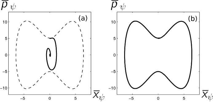
Figure 5: Time evolution of pointer states in an anharmonic fourth order potential (solid line). The dashed line shows the corresponding classical phase space trajectory. (a) The collision rate $\gamma$ vanishes leading to dispersive quantum dynamics. (b) The collision rate $\gamma$ is large, such that the dynamics of the pointer state is indistinguishable from the classical trajectory.      

In order to explain the numerical observation, first consider a particle in a linear potential $V\left(x\right)=\alpha x$. The corresponding nonlinear equation reads as

$$\partial_{t}\psi_{t}\left(x\right)\mbox{\rm}\mbox{\rm}+\frac{\hbar}{2mi}\partial_{x}^{2}\psi_{t}\left(x\right) = \frac{1}{i\hbar}\alpha x\psi_{t}\left(x\right)+\gamma\psi_{t}\left(x\right)\Bigl{[}|\psi_{t}|^{2}\ast\tilde{G}\left(x\right)$$ (48)

$$-\int^{\infty}_{-\infty}\mathrm{d}y|\psi_{t}|^{2}\left(y\right)\left(|\psi_{t}|^{2}\ast\hat{G}\right)\left(y\right)\Bigr{]}\,.$$

As discussed in Sect. 4.1, the field-free version of this equation $(\alpha=0)$ exhibits uniformly moving solitonic solutions of the form

$$\psi_{t}\left(x\right) = f\left(x-vt\right)\exp\left(i\left[\phi\left(x-vt\right)+\chi\left(t\right)\right]\right)\,.$$ (49)

This implies that (48) has solitonic solutions of the form

$$\psi_{t}\left(x\right) = f\left(x-x_{t}\right)\exp\left(ig\left(x-x_{t},t\right)\right)\,,$$ (50)

$$g\left(x,t\right) = \phi\left(x\right)+\chi^{\prime}\left(t\right)-\frac{\alpha}{\hbar}tx\,,$$ (51)

with $x_{t}=vt-\alpha t^{2}/2m\,$ and $\chi^{\prime}\left(t\right)=\chi\left(t\right)-2\alpha\int_{0}^{t}\mathrm{d}\tau\,x_{\tau}/\hbar$. In order to verify this statement, we evaluate the left hand side of (48) with the ansatz given by (50). This yields

$$\partial_{t}\psi_{t}\left(x\right)+\frac{\hbar}{2mi}\partial_{x}^{2}\psi_{t}\left(x\right) = e^{ig}\left(\frac{\alpha}{i\hbar}xf+if\partial_{t}\chi^{\prime}\left(t\right)+\frac{2\alpha}{\hbar}ix_{t}f-v\left(\partial_{x}f+if\partial_{x}\phi\right)\right.$$ (52)

$$\left.+\frac{\hbar}{m}\left(\partial_{x}f\partial_{x}\phi-\frac{i}{2}\partial_{x}^{2}f+\frac{i}{2}f\left(\partial_{x}\phi\right)^{2}+\frac{1}{2}f\partial_{x}^{2}\phi\right)\right)\,,$$

with $g\equiv g\left(x-x_{t},t\right)$, $f\equiv f\left(x-x_{t}\right)$ and $\phi\equiv\phi\left(x-x_{t}\right)$. The expression can be further simplified by noting that the free soliton (49) is a solution of the field-free version of (48), implying that

$$\gamma f\Lambda\left[f^{2}\right]\left(x\right) = if\partial_{t}\chi\left(t\right)-v\left(\partial_{x}f+if\partial_{x}\phi\right)$$ (53)

$$+\frac{\hbar}{m}\left(\partial_{x}f\partial_{x}\phi-\frac{i}{2}\partial_{x}^{2}f+\frac{i}{2}f\left(\partial_{x}\phi\right)^{2}+\frac{1}{2}f\partial_{x}^{2}\phi\right)\,,$$

with $\Lambda\left[f^{2}\right]\left(x\right)$ defined in (18). Using (52), (53) and the above definition of $\chi^{\prime}\left(t\right)$, one finds that

$$\partial_{t}\psi_{t}\left(x\right)+\frac{\hbar}{2mi}\partial_{x}^{2}\psi_{t}\left(x\right) = \frac{1}{i\hbar}\alpha x\psi_{t}\left(x\right)+\gamma\psi_{t}\left(x\right)\Lambda\left[\left|\psi_{t}\right|^{2}\right]\left(x\right)\,,$$ (54)

which confirms that $\psi_{t}\left(x\right)$ evolves according to (48).

We conclude that in a linear potential the pointer states have the same shape as in the field-free case and they are uniformly accelerated like a classical particle. For general potentials, this implies that the pointer states follow the corresponding classical motion, provided the spatial width of the solitons is sufficiently small, such that the linearization of the potential is justified over their spatial extension. Since the size of the pointer states decreases with the collision rate (see Section 4.3), the pointer states must exhibit classical dynamics in the limit of large collision rates.

5 Orthogonal Unraveling

Thus far, we have calculated ‘candidate’ pointer states as the solitonic solutions of (17), and we have studied their properties and dynamics. Next, it will be shown that these ‘candidates’ are genuine pointer states $\mathsf{P}_{\alpha}$ in the sense of (1). Moreover, we find that the statistical weights ${\rm Prob}\left(\alpha|\rho_{0}\right)$ of the pointer states are given by the overlap of the initial state $\rho_{0}$ with the initial pointer state $\mathsf{P}_{\alpha}\left(0\right)$, i.e.

$${\rm Prob}\left(\alpha|\rho_{0}\right) = {\rm Tr}\left[\rho_{0}\mathsf{P}_{\alpha}\left(0\right)\right]\,.$$ (55)

In order to verify the above conjectures, let us now make use of the formalism of quantum trajectories [15, 27, 21] to solve the master equation (13). More precisely, a specific quantum trajectory method, the orthogonal unraveling, is distinguished by the physics of pointer states because the deterministic part of the associated stochastic differential equation coincides with the nonlinear equation (11).

We start with a general description of the quantum trajectory approach and the orthogonal unraveling in Section 5.1. The latter will be applied to collisional decoherence in Section 5.2. This will allow us to evaluate the statistical weights of the pointer states in Section 5.3.

5.1 Quantum trajectories and the orthogonal unraveling

5.1.1 Quantum trajectories

In the quantum trajectory approach, the wave function corresponding to a pure initial state $|\psi\left(0\right)\rangle$ is propagated stochastically to generate pure state trajectories $\left\{|\psi_{i}\left(t\right)\rangle\right\}$, whose ensemble average recovers the solution of the master equation (12), i.e.

$$\exp\left(\mathcal{L}t\right)|\psi\left(0\right)\rangle\langle\psi\left(0\right)| = \mathbbm{E}\left(|\psi_{i}\left(t\right)\rangle\langle\psi_{i}\left(t\right)|\right)\,.$$ (56)

Such a stochastic process is called an unraveling of the master equation. A common unraveling is provided by the quantum Monte Carlo method [28, 29] which is based on a piecewise deterministic process. Here, one realization of a trajectory consists of smooth deterministic pieces generated by an effective (non-Hermitian) Hamiltonian, in our case

$$\mathsf{H}_{{\rm eff}} = \mathsf{H}-\frac{i\hbar}{2}\int_{-\infty}^{\infty}\mathrm{d}q\mathsf{L}_{q}^{{\dagger}}\mathsf{L}_{q}\,,$$ (57)

which are interrupted by random jumps. The jumps occur with the rate

$$r_{q} = \langle\mathsf{L}_{q}^{{\dagger}}\mathsf{L}_{q}\rangle\,,$$ (58)

an expectation value with respect to $|\psi_{i}\left(t\right)\rangle$, and they are effected by the operators

$$\mathsf{J}_{q} = \mathsf{L}_{q}/\sqrt{r_{q}}\,.$$ (59)

The quantum Monte Carlo method is not the only stochastic process satisfying (56). In fact, there exists an infinite set of these stochastic processes, because the convex decomposition of the density matrix on the left hand side of (56) is not unique. For instance, other unravelings can be obtained from the quantum Monte Carlo method, by noting that the generator $\mathcal{L}$ does not uniquely fix the Lindblad operators $\mathsf{L}_{q}\,$ and the Hamiltonian $\mathsf{H}$ [29, 21]. This is due to the fact that the master equation (12) is invariant under certain transformations of the Lindblad operators, such as the addition of a complex multiple $z_{q}$ of the identity $\mathsf{\mathsf{\mathsf{\mathsf{I}}}}$,

$$\mathsf{L}_{q} \rightarrow \mathsf{L}_{q}^{\prime}=\mathsf{L}_{q}+z_{q}\mathsf{I}\,.$$ (60)

In the latter case, also the Hamiltonian must be transformed as

$$\mathsf{H} \rightarrow \mathsf{H}^{\prime}=\mathsf{H}+\frac{1}{2i}\int_{-\infty}^{\infty}\mathrm{d}q\left(z_{q}^{\ast}\mathsf{L}_{q}-z_{q}\mathsf{L}_{q}^{{\dagger}}\right)\,,$$ (61)

in order to assure the invariance of the master equation.

5.1.2 The orthogonal unraveling

To obtain a different, but again piecewise deterministic unraveling, we now make the choice $z_{q}=-\langle\mathsf{L}_{q}\rangle$. It then follows that the deterministic pieces of a sample path are given by the solution of the nonlinear equation (16) (or equivalently the corresponding projector equation (11)). The jumps occur with the rate

$$r_{q} = \langle\mathsf{L}_{q}^{{\dagger}}\mathsf{L}_{q}\rangle-\langle\mathsf{L}_{q}^{{\dagger}}\rangle\langle\mathsf{L}_{q}\rangle\,,$$ (62)

and are caused by the nonlinear operators

$$\mathsf{J}_{q} = \left(\mathsf{L}_{q}-\langle\mathsf{L}_{q}\rangle\right)/\sqrt{r_{q}}\,.$$ (63)

As a distinctive feature, the states $|\psi_{q}\left(t\right)\rangle=\mathsf{J}_{q}|\psi\left(t\right)\rangle$ into which the system may jump are orthogonal to the original state $|\psi\left(t\right)\rangle$, thus justifying its naming. (The states $|\psi_{q}\left(t\right)\rangle$ are not necessarily mutually orthogonal, though.) To our knowledge, this unraveling was first noted by Rigo and Gisin [16], although, it has not been studied numerically so far.

A related unraveling, which is also referred to as the ‘orthogonal unraveling’, was introduced by Diósi [30, 15]. Here, the deterministic pieces of the evolution are as well generated by (16). However, the states $|\psi_{q}\left(t\right)\rangle$ into which the system may jump are obtained differently, as the eigenvectors of the Hermitian operator

$$\left(1-\mathsf{P}_{\psi\left(t\right)}\right)\mathcal{L}\left(\mathsf{P}_{\psi\left(t\right)})\left(1-\mathsf{P}_{\psi\left(t\right)}\right)\,,\right.$$ (64)

where $\mathsf{P}_{\psi\left(t\right)}\equiv|\psi\left(t\right)\rangle\langle\psi\left(t\right)|$. As a consequence, these states are also mutually orthogonal (in finite dimensional systems). Since the orthogonal unraveling of [30, 15] requires the diagonalization of the operator (64), it is much more involved than the one defined by (16), (62) and (63), which is why we will use the latter in the following.

5.1.3 Pointer states and the orthogonal unraveling

As mentioned above, all unravelings are equivalent in the same sense as the different convex decompositions of the density matrix $e^{\mathcal{L}t}\rho_{0}$. Note, however, that a preferred set of pure states – the pointer basis – may be singled out through the environmental coupling. In that case, those unravelings are distinguished which generate for any initial state an ensemble of these state independent projectors. An unraveling will do this job if (a) its deterministic part exhibits stable fixed points or solitons $\mathsf{P}_{\alpha}=|\pi_{\alpha}\rangle\langle\pi_{\alpha}|$, which (b) are characterized by a vanishing jump rate, $r\left(\mathsf{P}_{\alpha}\right)=0\,$. In that case, the sample paths of the process will end up in one of the states $\mathsf{P}_{\alpha}$, by all means. Hence, the ensemble mean is of the form (3), such that the fixed points or solitons $\mathsf{P}_{\alpha}$ can be identified with the pointer states of the system.

For the case of collisional decoherence the orthogonal unraveling fulfills the aforesaid conditions. (a) Its deterministic part is given by (17) which exhibits the solitonic solutions $\pi\left(x\right)$ shown in Fig. 2. We shall see explicitly in Section 5.2.1 that these states are attractive fixed points. (b) We will show in Section 5.2.2 that the jump rate (62) vanishes for the solitons $\pi\left(x\right)$, which finally demonstrates that our ‘candidate’ pointer states $\pi\left(x\right)$ are genuine pointer states $\mathsf{P}_{\alpha}$ in the sense of (1). Moreover, this shows that the orthogonal unraveling is a very efficient numerical scheme for the long time solution of the master equation (13), since the state is no longer affected by the stochastic part, once it has turned into the soliton, and the trajectory is therefore more easy to integrate.

We note that the orthogonal unraveling is not the only stochastic process which generates the ensemble of pointer states. In fact, there is a diffusive unraveling [31], which also involves (11) as its deterministic part. It was applied in [6] to investigate pointer states in a linear model.

5.2 Unraveling collisional decoherence

We now apply the described orthogonal unraveling to collisional decoherence (13), first evaluating the deterministic part (16) of the stochastic process in Sect. 5.2.1 and then the stochastic one (62) and (63) in Sect. 5.2.2.

5.2.1 Deterministic evolution

Applying (16) to the case of collisional decoherence yields the soliton equation (17) discussed in Sect. 3.2. We will now further simplify this equation, by considering initial states

$$\Psi_{0}\left(x\right) = \sum_{i=1}^{N}c_{i}\left(0\right)\phi_{i}\left(x,0\right)\,,$$ (65)

which are superpositions of non-overlapping wave functions $\phi_{i}\left(x,0\right)$,

$$\phi_{i}\left(x,0\right)\phi_{j\neq i}^{\ast}\left(x,0\right) = 0\,.$$ (66)

The latter are assumed to be localized in the sense that

$$\sigma^{2}_{\phi_{i}} < \frac{2\pi\hbar^{2}}{\sigma_{G}^{2}}\,,$$ (67)

where $\sigma^{2}_{\phi_{i}}$ and $\sigma_{G}^{2}$ denote the variances of the distributions $\left|\phi_{i}\left(x,0\right)\right|^{2}$ and $G\left(q\right)$, respectively. Under this assumption, which will be justified at the end of this section, one can extract a system of evolution equations for the time evolution of the coefficients in (65),

$$\frac{\mathrm{d}}{\mathrm{d}t}c_{i}\left(t\right)=-\left(\sum_{j=1}^{N}F_{ij}\left|c_{j}\left(t\right)\right|^{2}-\sum_{j,k=1}^{N}F_{jk}\left|c_{j}\left(t\right)\right|^{2}\left|c_{k}\left(t\right)\right|^{2}\right)c_{i}\left(t\right)\,.$$ (68)

Here, the matrix $F_{ij}\equiv F\left(x_{i}-x_{j}\right)$ is obtained from the localization rate (15), where the $x_{i}\equiv\langle\mathsf{x}\rangle_{\phi_{i}}$ denote the mean positions of the constituent wave functions $\phi_{i}\left(x,t\right)$. The latter evolve according to

$$\partial_{t}\phi_{i}\left(x,t\right) = -\frac{\hbar}{2\,m\,i}\partial_{x}^{2}\phi_{i}\left(x,t\right)+\phi_{i}\left(x,t\right)\Lambda\left[\left|\phi_{i}\right|^{2}\right]\left(x,t\right)$$ (69)

$$+\phi_{i}(x,t)\sum^{N}_{j=1,j\neq i}\left|c_{j}\left(t\right)\right|^{2}\tilde{\gamma}_{ij}\left(x,t\right)\,,$$

where $\Lambda$ is defined in (18) and $\tilde{\gamma}_{ij}$ is a rate of the order of $\gamma$,

$$\tilde{\gamma}_{ij}\left(x,t\right) \equiv \left|\phi_{i}\right|^{2}\ast F\left(x,t\right)-\left|\phi_{j}\right|^{2}\ast F\left(x,t\right)+F_{ij}\,.$$ (70)

Let us now verify that $\Psi_{t}\left(x\right)=\sum_{i=1}^{N}c_{i}\left(t\right)\phi_{i}\left(x,t\right)$, with $c_{i}\left(t\right)$ and $\phi_{i}\left(x,t\right)$ solutions of (68) and (69), evolves according to (17). First, we note that the assumption (67) leads to the approximation

$$\int_{-\infty}^{\infty}\mathrm{d}x\left|\phi_{i}\left(x\right)\right|^{2}e^{iqx/\hbar} \simeq e^{iqx_{i}/\hbar}\,,$$ (71)

for all $q$ contributing appreciably to integrals weighted with the momentum transfer distribution $G\left(q\right)$. This, in turn, implies

$$F_{jk} = F\left(x_{j}-x_{k}\right)$$

$$\simeq \int_{-\infty}^{\infty}\mathrm{d}x\left|\phi_{j}\left(x\right)\right|^{2}\left(\left|\phi_{k}\right|^{2}\ast F\right)\left(x\right)\,.$$

Hence, we find that $\int_{-\infty}^{\infty}\mathrm{d}x\left|\phi_{i}\left(x\right)\right|^{2}\left(\left|\phi_{i}\right|^{2}\ast F\right)\left(x\right)\simeq 0$, and one thus obtains

$$\Lambda\left[\left|\phi_{i}\right|^{2}\right]\left(x,t\right) = -\left(\left|\phi_{i}\right|^{2}\ast F\right)\left(x,t\right)\,.$$ (73)

Now, consider the time derivative of $\Psi_{t}\left(x\right)$, which gives

$$\partial_{t}\Psi = -\frac{\hbar}{2\,m\,i}\sum_{i=1}^{N}c_{i}\partial_{x}^{2}\phi_{i}-\left(\sum_{i=1}^{N}c_{i}\phi_{i}\right)\,$$ (74)

$$\times\left(\sum_{j=1}^{N}\left|c_{j}\right|^{2}\left(\left|\phi_{j}\right|^{2}\ast F\right)-\sum_{j,k=1}^{N}\left|c_{j}\right|^{2}\left|c_{k}\right|^{2}F_{jk}\right)\,,$$

where we dropped the arguments for brevity. In (74), we used (68)-(70), (73), the fact that $F_{ii}=0$, and the normalization condition $\sum_{i=1}^{N}\left|c_{i}\right|^{2}=1$. Now, we replace $F_{jk}$ in (74) by the right hand side of (5.2.1), and use (66), which yields

$$\partial_{t}\Psi_{t}\left(x\right) = -\frac{\hbar}{2mi}\partial_{x}^{2}\Psi_{t}\left(x\right)-\Psi_{t}\left(x\right)\Bigl{(}|\Psi_{t}|^{2}\ast F\left(x\right)$$ (75)

$$-\int_{-\infty}^{\infty}\mathrm{d}x|\Psi_{t}|^{2}\left(y\right)\left(|\Psi_{t}|^{2}\ast F\right)\left(y\right)\Bigr{)}\,.$$

Finally, by using (15), we obtain

$$\partial_{t}\Psi_{t}\left(x\right) = -\frac{\hbar}{2mi}\partial_{x}^{2}\Psi_{t}+\gamma\Psi_{t}\left(x\right)$$

$$\times\left(|\Psi_{t}|^{2}\ast\hat{G}\left(x\right)-\int^{\infty}_{-\infty}\mathrm{d}y|\Psi_{t}|^{2}\left(y\right)\left(|\Psi_{t}|^{2}\ast\hat{G}\right)\left(y\right)\right)\,,$$

which confirms that $\Psi_{t}\left(x\right)$ evolves according to (17).

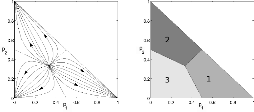
Figure 6: Numerical solution of (68) for $N=3$. The $x$-axis gives $p_{1}=\left|c_{1}\right|^{2}$, the $y$-axis $p_{2}=\left|c_{2}\right|^{2}$, and $\left|c_{3}\right|^{2}$ is fixed by normalization. Left: trajectories indicating the flow into the stable fixed points $\left|c_{i}\right|=\delta_{i,n},\left(n=1,2,3\right)$. Right: regions of attraction of the stable fixed points; the area denoted with $n$ is the region of attraction of the fixed point $\left|c_{i}\right|=\delta_{i,n}\,.$   

Let us now discuss the solution of Eq. (68) for the time evolution of the coefficients. We first consider situations where the wave packets $\phi_{i}\left(x\right)$ are sufficiently far apart such that the localization rate is saturated, i.e. $F_{ij}=\gamma\left(1-\delta_{ij}\right).$ Under this assumption, (68) reduces to the equation

$$\frac{\mathrm{d}}{\mathrm{d}t}c_{i}\left(t\right) = -\gamma\left(\sum_{j=1}^{N}\left|c_{j}\left(t\right)\right|^{4}-|c_{i}\left(t\right)|^{2}\right)c_{i}\left(t\right)\,,$$ (77)

which was already studied in [32] in the context of a discrete model for quantum measurement. It is shown there that all stable fixed points of (77) have the form $\left|c_{i}\right|=\delta_{i,n}\,$, and that the particular fixed point $\left|c_{i}\right|=\delta_{i,m}\,$, with

$$m = \max_{i}\left(\left|c_{i}\left(0\right)\right|^{2}\right)$$ arg , (78)

is approached monotonically, i.e. the component with the largest initial weight wins. This behavior is visualized in Fig. 6 which was obtained by solving (77) numerically for the case $N=3$. Here, the $x$- and the $y$-axis indicate the weights $p_{1}=\left|c_{1}\right|^{2}$ and $p_{2}=\left|c_{2}\right|^{2}$, respectively. The plot on the left hand side shows various trajectories, illustrating in particular the fixed points. The plot on the right displays the regions of attraction of the stable fixed points $\left|c_{i}\right|=\delta_{i,n}$, in agreement with the criterion (78). For instance, area $1$ highlights the region of attraction of the fixed point $\left|c_{i}\right|=\delta_{i,1}$.

Figure 7, on the other hand, depicts a scenario where the wave packets $\phi_{i}\left(x\right)$ are close together such that the localization rate is unsaturated, i.e. $F_{ij}\leqslant\gamma\left(1-\delta_{ij}\right)$. Here, we choose $N=3$ wave packets with non-equidistant position expectations, $\left(x_{1},x_{2},x_{3}\right)\sigma_{G}/\hbar=\left(1.4,1.3,0.8\right)$. Similarly to the saturated case, we observe that all stable fixed points of (68) have the form $\left|c_{i}\right|=\delta_{i,n}\,$. However, the regions of attraction are deformed such that criterion (78) is no longer valid, and the fixed points are not necessarily approached monotonically.

To see that $\left|c_{i}\right|=\delta_{i,n}\,$ are stable fixed points of (68), assume that the coefficients are close by, i.e. $\left|c_{n}\left(t\right)\right|=1-\varepsilon\left(t\right)$ with $\varepsilon\left(0\right)\ll 1$. It follows from (68) that

$$\dot{\varepsilon}\left(t\right) = -\sum_{j}F_{nj}\,\left|c_{j}\left(t\right)\right|^{2}+O\left(\varepsilon^{2}\right)\><\>0\,,$$ (79)

and hence, $\left|c_{i}\left(t\rightarrow\infty\right)\right|=\delta_{i,n}$.

The knowledge of the fixed points of the coefficients allows one to discuss the asymptotic evolution of the initial state shown in Eq. (65). Since the coefficients $c_{j}$ with $j\neq m\,$ tend to zero asymptotically, it follows that

$$|\psi\left(t\rightarrow\infty\right)\rangle = |\phi_{m}\left(t\rightarrow\infty\right)\rangle\,,$$ (80)

for a specific $m$ (which is given by (78) in the saturated case). The asymptotic behavior of the wave packets $|\phi_{m}\rangle$ can, in turn, be predicted from Eq. (69). Since the $c_{j\neq m}$ vanish for large times, the coupling term given by the last summand in (69) vanishes as well, implying that the time evolution (69) of $|\phi_{m}\rangle$ is asymptotically equal to the soliton equation (17). Therefore, in the absence of stochastic jumps, the state $|\Psi_{0}\rangle$ evolves into that solitonic solution $\pi_{m}\left(x\right)$ of (17) which is associated to the initial wave packet $|\phi_{m}\left(0\right)\rangle$.

It should be mentioned that Eqs. (68) and (69) for the coefficients $c_{i}$ and the constituent wave packets $\phi_{i}$ are not completely decoupled, since (68) depends on the matrix $F_{ij}\equiv F\left(x_{i}-x_{j}\right)$ which contains the position expectations $x_{i}$ of the wave packets $\phi_{i}$. However, the position expectation follows the classical trajectory for sufficiently large $\kappa$’s, such that (68) can be solved without knowing the solution of (69).

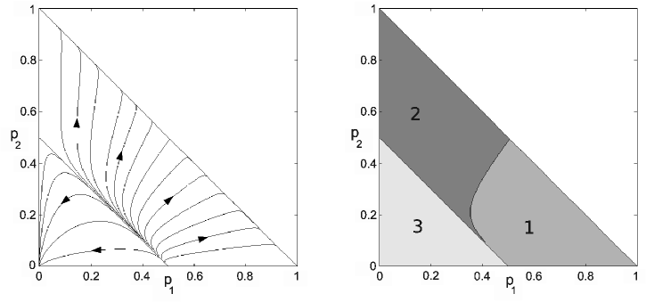
Figure 7: Similar to Fig. 6, but the wave packets $\phi_{i}\left(x\right)$ are positioned closer such that the localization rate is unsaturated, i.e. $F_{ij}\leqslant\gamma\left(1-\delta_{ij}\right)$. The stable fixed points are still of the form $\left|c_{i}\right|=\delta_{i,n}$, but they may be approached non-monotonically and the regions of attraction, shown on the right, are deformed compared to the saturated case.

Let us now discuss the validity of the assumption of small position variance (67), and the ensuing approximation (71). It can be justified by our observation in Section 4.3, that the dimensionless pointer width $\sigma_{\pi}\sigma_{G}/\hbar$ is a function of the parameter $\kappa\equiv\sigma_{G}^{2}/m\hbar\gamma$ only,

$$\sigma_{\pi}\frac{\sigma_{G}}{\hbar} = \frac{\kappa}{4a_{{\rm loc}}}+a_{{\rm loc}}\,,\hskip 20.00003pt{\rm with}\,\,a_{{\rm loc}}=0.4\,.$$ (81)

Thus, for all $\kappa\ll 4a^{2}_{{\rm loc}}\simeq 1$ we find that the position variance $\sigma_{\pi}^{2}$ of a pointer state is one order of magnitude smaller than the reciprocal width of the momentum transfer distribution $G\left(q\right)$,

$$\mbox{\rm$\sigma_{\pi}^{2}$}\simeq a_{{\rm loc}}^{2}\frac{\hbar^{2}}{\sigma_{G}^{2}}\simeq 0.2\frac{\hbar^{2}}{\sigma_{G}^{2}}<2\pi\frac{\hbar^{2}}{\sigma_{G}^{2}}\,.$$ (82)

The above relation for the width of the pointer state is sufficient to justify the approximation $\int\mathrm{d}xe^{iqx/\hbar}\left|\pi\left(x\right)\right|^{2}\simeq e^{iq\langle\mathsf{x}\rangle_{\pi}/\hbar}$, as we checked numerically, by using the solitonic solution of (6). The relative error is less than $2\%$ for $q\in\left[-2\sigma_{G},2\sigma_{G}\right]$ and $\kappa\leqslant 10^{-3}$.

5.2.2 Stochastic part

Upon inserting the Lindblad operator $\mathsf{L}_{q}=\sqrt{\gamma G\left(q\right)}e^{iq\mathsf{x}}$ into (63) we find that the jump operator takes the form

$$\mathsf{J}_{q} = \mathcal{N}_{q}\,\left(e^{iq\mathsf{x}/\hbar}-\langle e^{iq\mathsf{x}/\hbar}\rangle\right)\,,$$ (83)

with normalization $\mathcal{N}_{q}=\left(1-|\langle e^{iq\mathsf{x}/\hbar}\rangle|^{2}\right)^{-1/2}$. We again consider states of the form (65) which are superpositions of non-overlapping (66) and localized (67) wave packets $\phi_{i}\left(x\right)$. Under this assumption, one can evaluate the expectation value in (83)

$$\langle e^{iq\mathsf{x}/\hbar}\rangle_{\Psi} = \sum_{i=1}^{N}\left|c_{j}\right|^{2}e^{iqx_{j}/\hbar}\,,$$ (84)

such that the state $\Psi_{q}\left(x\right)\equiv\mathsf{J}_{q}\Psi\left(x\right)$ into which the system may jump takes the form

$$\Psi_{q}\left(x\right) = \mathcal{N}_{q}\left(e^{iqx/\hbar}-\sum_{i=1}^{N}\left|c_{j}\right|^{2}e^{iqx_{j}/\hbar}\right)\sum_{i=1}^{N}c_{i}\,\phi_{i}\left(x\right)\,.$$ (85)

Later we will choose the initial wave packets $\phi_{i}\left(x\right)$ to be solitons $\pi_{i}\left(x\right)$. Let us therefore assume that the $\phi_{i}$’s form a basis, such that $\Psi_{q}\left(x\right)$ can be represented as $\Psi_{q}\left(x\right)=\sum_{i}c_{i}\left(q\right)\phi_{i}\left(x\right)\,$. Then the transformed coefficients $c_{k}\left(q\right)$ can be evaluated by the overlap $c_{k}\left(q\right)=\langle\phi_{k}|\mathsf{J}_{q}|\Psi\rangle$. Using (66) and (71) this leads to the following expression for the redistribution of the coefficients due to an orthogonal jump

$$c_{k}\left(q\right) = \mathcal{N}_{q}\left(e^{iqx_{k}/\hbar}-\sum_{i=1}^{N}\left|c_{i}\right|^{2}e^{iqx_{i}/\hbar}\right)c_{k}\,,$$ (86)

Similarly, one can evaluate the rate (62) associated to the jump operator of collisional decoherence,

$$r_{q} = \gamma\,G\left(q\right)\left(1-|\langle e^{iq\mathsf{x}/\hbar}\rangle|^{2}\right)\,.$$ (87)

The above approximation (84) further simplifies this expression,

$$r_{q} = \gamma\,G\left(q\right)\left(1-\sum_{j,k=1}^{N}\left|c_{j}\right|^{2}\left|c_{k}\right|^{2}e^{iq\left(x_{j}-x_{k}\right)/\hbar}\right)\,.$$ (88)

One observes that this rate vanishes for the stable fixed points $\left|c_{i}\right|=\delta_{i,n}$, indicating that the quantum trajectories of the orthogonal unraveling evolve into the pointer states, the solitonic solutions of (17). Moreover, we note that the original stochastic process (16), (62), (63) – which is defined in the infinite dimensional Hilbert space of the system – has been reduced to a stochastic process in $\mathbbm{C}^{N}$, demonstrating the efficiency of the orthogonal unraveling. However, due to the finite pointer width (37) the exact expression for the jump rate (87) does not vanish identically, although it is very small compared to $\gamma$. For instance, the numerically obtained soliton displays a strongly suppressed total jump rate $r_{{\rm tot}}=\int\mathrm{d}q\,r_{q}$ of $r_{{\rm tot}}/\gamma=7\times 10^{-3}$ for $\kappa=10^{-3}$, while the superposition state decays with the rate $r_{{\rm tot}}\cong\gamma$. This implies that the solitons are not perfect pure state solutions of the master equation (13), though the loss of purity is small.

5.3 The statistical weights of the pointer states

The previous section showed that the orthogonal unraveling of an initial superposition state subject to collisional decoherence can be reduced to a stochastic process with respect to the corresponding coefficients. In particular, this applies to the case where the initial state is a superposition of pointer states,

$$|\Psi_{0}\rangle = \sum_{i=1}^{N}c_{i}|\pi_{i}\left(0\right)\rangle\,.$$ (89)

Thus we can now verify, by using the discrete process defined by Eqs. (68), (86) and (88), that after decoherence the statistical weights of the pointer states are given by the overlap of the initial state with the initial pointer states. More specifically, this demonstrates that the initial state $\Psi_{0}\left(x\right)$ evolves into the mixture

$$\rho\left(x,x^{\prime}\right) = \sum_{i=1}^{N}p_{i}\pi_{i}\left(x\right)\pi_{i}^{\ast}\left(x^{\prime}\right)\,,$$ (90)

where the statistical weights are given by the overlap

$$p_{i} = \left|\langle\Psi_{0}|\pi_{i}\left(x,0\right)\rangle\right|^{2}\,.$$ (91)

We first present an analytic proof of the above for $N=2\,$. The general case, $N>2\,$, is then treated numerically in the following section.

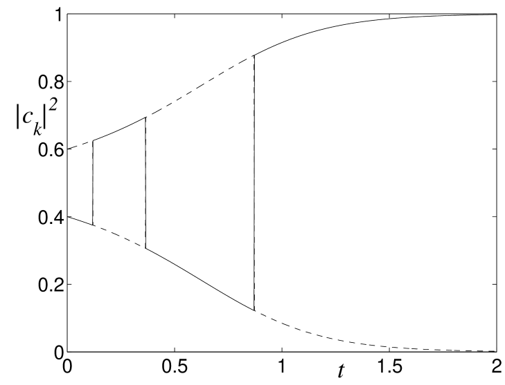
Figure 8: Quantum trajectory generated by (68), (93) and (94) with $N=2\,$. The solid line depicts the evolution of $\left|c_{1}\left(t\right)\right|^{2}\,$, while the dashed line shows $\left|c_{2}\left(t\right)\right|^{2}$. Since there is an odd number of jumps (three jumps in this example), the trajectory evolves into the fixed point $\left|c_{i}\right|=\delta_{i,1}$.

5.3.1 Superposition of two localized states

We consider the expectation value for the coefficients after a jump, that is

$$\langle c_{k}\left(q\right)\rangle_{G} := \int_{-\infty}^{\infty}\mathrm{d}q\,G\left(q\right)c_{k}\left(q\right)\,,\hskip 20.00003ptk=1,2\,.$$ (92)

Upon inserting (86) one obtains $\langle c_{1}\left(q\right)\rangle_{G}=\mathcal{N}^{\prime}\left|c_{2}\right|^{2}c_{1}$, with the normalization constant $\mathcal{N}^{\prime}=\langle\mathcal{N}_{q}\left(e^{iqx_{1}/\hbar}-e^{iqx_{2}/\hbar}\right)\rangle_{G}\,$, see (83). Using $\left|\langle c_{1}\left(q\right)\rangle_{G}\right|^{2}+\left|\langle c_{2}\left(q\right)\rangle_{G}\right|^{2}=1$, we find $\left|\mathcal{N}^{\prime}\right|=1/\left(\left|c_{1}c_{2}\right|\right)$ which implies

$$\left|\langle c_{1}\left(q\right)\rangle_{G}\right| = \left|c_{2}\right|\,.$$ (93)

This shows that after an average jump the moduli of the coefficients are simply interchanged. This property (which does not hold for $N>2$) makes the stochastic process analytically tractable, not least because the dynamics is independent of the phases of the coefficients. Since the deterministic part (68) of the evolution is monotonic for $N=2$, a trajectory starting from $\left|c_{1}\left(0\right)\right|<1/2$ will end up in the state $\left|c_{i}\left(\infty\right)\right|=\delta_{i,1}$ if and only if an odd number of jumps occurs in the process. This is demonstrated in Fig. 8. Crucially, the jump rate $r_{{\rm tot}}\,\left(t\right)$,

$$r_{{\rm tot}}\left(t\right) := \int_{-\infty}^{\infty}\mathrm{d}qr_{q}\left(t\right)$$ (94)

$$= 2F\left(x_{1}-x_{2}\right)\left|c_{1}\left(t\right)\right|^{2}\left|c_{2}\left(t\right)\right|^{2}\,,$$

is unaffected by the jump (93) at all times, since it is invariant under interchanging the coefficients. Hence, the time dependence of the jump rate is identical for all trajectories, which, in turn, means that the number of jumps follows an inhomogeneous Poisson process. Therefore, the probability for an odd number of jumps, which is equal to the statistical weight $p_{1}$ of the pointer state $\pi_{1}\left(x\right)$, is given by

$${\rm Prob}\left({\rm odd}\right) = \left(1-e^{-2\mu\left(\infty\right)}/2\right)\,,$$ (95)

with $\mu\left(t\right)=\int_{0}^{t}\mathrm{d}\tau\,r_{{\rm tot}}\left(\tau\right)$ the integrated jump rate. The latter can easily be evaluated by noting that (68) can be written for $N=2$ as

$$2F\left(x_{1}-x_{2}\right)\left|c_{1}\left(\tau\right)\right|^{2}\left|c_{2}\left(\tau\right)\right|^{2} = \frac{1}{2}\frac{\mathrm{d}}{\mathrm{d}t}\ln\left(1-2\left|c_{1}\left(\tau\right)\right|^{2}\right)\,.$$ (96)

Upon inserting this result into (94) we obtain the integrated jump rate:

$$\mu\left(\infty\right) = \int_{0}^{\infty}\mathrm{d}\tau\frac{1}{2}\frac{\mathrm{d}}{\mathrm{d}t}\ln\left(1-2\left|c_{1}\left(\tau\right)\right|^{2}\right)\,$$ (97)

$$= -\ln\left(1-2\left|c_{1}\left(0\right)\right|^{2}\right)/2\,.$$

Noting (95) we thus find the probability for an odd number of jumps

$${\rm Prob}\left({\rm odd}\right) = \left|c_{1}\left(0\right)\right|^{2}\,.$$ (98)

This finally confirms that the statistical weights of the pointer states are indeed given by the expected overlap (91).

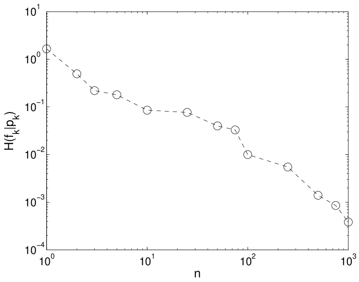
Figure 9: Relative entropy $H\left(f_{k}|p_{k}\right)$ of the numerically obtained distribution of pointer states $f_{k}$ with respect to the expected distribution $p_{k}=\left|c_{k}\right|^{2}$ as a function of the number of trajectories $n$ generated in the simulation. The plot indicates that the pointer states are distributed according to the initial overlap $\left|c_{k}\right|^{2}$.

5.3.2 Superposition of $N>2$ localized states

The stochastic process is much more involved if the initial superposition consists of more than two pointer states. Our numerical implementation of the stochastic process defined by (68), (86) and (88) is based on a Metropolis-Hastings algorithm to draw the momentum transfer $q$ in accordance with the rate (88), with $G\left(q\right)$ a Gaussian. Each of the generated trajectories ends asymptotically in one of the fixed points corresponding to a pointer state, and we thus obtain a numerical estimate of the statistical weights by means of the relative frequencies $f_{k}\>,\,1\leqslant k\leqslant N$, of the asymptotic states. To confirm the expected probability distribution $p_{k}=\left|c_{k}\left(0\right)\right|^{2}$, we evaluate the relative entropy $H\left(f_{k}|p_{k}\right)$ between these two distributions. Figure 9 shows the result for a random initial state with $N=5$ as a function of the number of trajectories $n$, indicating convergence to zero. In addition, we found for $100$ random initial states, with random $2<N<11$, based on $10^{4}$ trajectories that the relative entropy was always less than $4\times 10^{-3}$. This holds both for cases where the initial wave packets $\pi_{i}\left(x\right)$ are far apart such that the localization rate is saturated, $F\left(x_{i}-x_{j}\right)\simeq\gamma$, and for situations where the wave packets are located close together such that $F\left(x_{i}-x_{j}\right)<\gamma$. We conclude that the asymptotic trajectories are indeed distributed according to the expected overlap (91).

As an alternative confirmation of the statistical weights, we performed a $\chi^{2}$-test. Similar to the treatment above, $100$ random initial states $\left\{\Psi_{i}|\,1\leqslant i\leqslant 100\right\}\,$, with random $2<N<11$, were drawn by the simplex picking method. For each random state, $n=100$ trajectories were generated, each of which ends asymptotically in one of the pointer states. Using the observed relative frequencies $f_{k}\>,\,1\leqslant k\leqslant N$, of the pointer states, we evaluate

$$\chi^{2} = n\sum_{k=1}^{N}\frac{\left(f_{k}-\left|c_{k}\left(0\right)\right|^{2}\right)^{2}}{\left|c_{k}\left(0\right)\right|^{2}}\,,$$ (99)

for each random state. In order to verify that the pointer states are distributed according to $\left|c_{k}\left(0\right)\right|^{2}$, the set $\left\{\chi_{i}^{2}\right\}$ must be shown to be sampled from a $\chi^{2}$-distribution with $N-1$ degrees of freedom. Comparing the set $\left\{\chi_{i}^{2}\right\}$ with the $\alpha$-quantiles (denoted by $Q_{\alpha}$) of the corresponding $\chi^{2}$-distribution, a typical run shows ten cases where $\chi_{i}^{2}>Q_{0.9\,}$, one case where $\chi_{i}^{2}>\mbox{\rm$Q_{0.99}$}$, but not a single case where $\chi_{i}^{2}>\mbox{\rm$Q_{0.999}$}$, as one expects if the $\left\{\chi_{i}^{2}\right\}$ are $\chi^{2}$-distributed. Like above, this confirms statistically that the asymptotic trajectories are distributed according to the expected overlap (91).

6 Conclusion

In this article, we related the nonlinear pure state equation discussed in [6, 7, 8] to a specific orthogonal unraveling of the collisional decoherence master equation. This puts into evidence that the dynamics of a particle in an ideal gas environment can be represented by an ensemble of pure state trajectories which evolve into spatially localized pointer states. For sufficiently strong collisions with the background gas, these solitonic wave packets move according to the classical equations of motion, thus explaining the emergence of classical dynamics within the quantum framework.

Once the pointer state is reached by an individual quantum trajectory, the latter is no longer affected by the stochastic part of the unraveling, such that the integration of the trajectory is reduced to the solution of the classical equations of motion. This suggests that the orthogonal unraveling is an efficient algorithm for the long time solution of master equations which exhibit a pointer basis. On the other hand, also the short time solution turns out to be efficient, since the orthogonal unraveling can be reduced (under appropriate assumptions) from an infinite dimensional unraveling to a stochastic process in $\mathbbm{C}^{N}$.

Future studies might consider the emergence and dynamics of pointer states in dissipative quantum systems. We note that the present work relies on the model of pure collisional decoherence which does not describe long time effects such as dissipation or thermalization. It would certainly be worth to determine the pointer states of a more involved model such as the quantum linear Boltzmann equation presented in [33, 34, 35]. For large mass ratios between the test particle and the gas, one expects that the pointer states then evolve according to a Langevin equation, thus explaining the emergence of classical Brownian motion within the quantum framework.

We thank B. Vacchini for helpful discussions. The work was supported by the DFG Emmy Noether program.

References

- [1] E. Joos and H. D. Zeh, Z. Phys. B: Condens. Matter 59, 223–243 (1985).
- [2] M. Schlosshauer, Decoherence and the Quantum-To-Classical Transition, Springer, Berlin, 2007.
- [3] W. H. Zurek, Rev. Mod. Phys. 75, 715–775 (2003).
- [4] W. H. Zurek, Phys. Rev. D 24, 1516–1525 (1981).
- [5] W. H. Zurek, S. Habib, and J. P. Paz, Phys. Rev. Lett. 70, 1187–1190 (1993).
- [6] L. Diósi and C. Kiefer, Phys. Rev. Lett. 85, 3552–3555 (2000).
- [7] N. Gisin and M. Rigo, J. Phys. A: Math. Gen. 28, 7375–7390 (1995).
- [8] W. T. Strunz, Lect. Notes Phys. 611, 199–233 (2002).
- [9] J. Eisert, Phys. Rev. Lett. 92, 210401 (2004).
- [10] K. Hornberger, S. Uttenthaler, B. Brezger, L. Hackermüller, M. Arndt, and A. Zeilinger, Phys. Rev. Lett. 90, 160401 (2003).
- [11] L. Hackermüller, K. Hornberger, B. Brezger, A. Zeilinger, M. Arndt, Appl. Phys. B 77, 781–787 (2003).
- [12] K. Hornberger, J. E. Sipe, and M. Arndt, Phys. Rev. A 70, 053608 (2004).
- [13] B. Vacchini, J. Mod. Opt. 51, 1025–1029 (2004).
- [14] B. Vacchini, Phys. Rev. Lett. 95, 230402 (2005).
- [15] L. Diósi, Phys. Lett. 114A, 451–454 (1986).
- [16] M. Rigo and N. Gisin, Quantum Semiclass. Opt. 8, 255–268 (1996).
- [17] M. Busse and K. Hornberger, J. Phys. A: Math. Gen. 42, 362001 (2009).
- [18] G. C. Ghirardi, A. Rimini, and T. Weber, Phys. Rev. D 34, 470–491 (1986).
- [19] A. Bassi and G. Ghirardi, Phys. Rep. 379, 257–426 (2003).
- [20] B. Vacchini, J. Phys. A: Math. Gen. 40, 2463–2473 (2007).
- [21] H.-P. Breuer and F. Petruccione, The Theory of Open Quantum Systems, Oxford University Press, Oxford, 2007.
- [22] K. Hornberger, Introduction to Decoherence Theory, in: Entanglement and Decoherence. Foundations and Modern Trends, ed. by A. Buchleitner, C. Viviescas, and M. Tiersch, Lect. Notes Phys. 768, 221–276, Springer, Berlin, 2009.
- [23] M. R. Gallis and G. N. Fleming, Phys. Rev. A 42, 38–48 (1990).
- [24] K. Hornberger and J. E. Sipe, Phys. Rev. A 68, 012105 (2003).
- [25] J. Eisert, M. B. Plenio, S. Bose, and J. Hartley, Phys. Rev. Lett. 93, 190402 (2004).
- [26] J. Klauder and B. Skagerstam, J. Phys. A: Math. Gen. 40, 2093 (2007).
- [27] H. Carmichael, An Open Systems Approach to Quantum Optics, Springer, Berlin, 1993.
- [28] K. Mølmer, Y. Castin, and J. Dalibard, J. Opt. Soc. Am. B 10, 524–538 (1993).
- [29] K. Mølmer and Y. Castin, Quantum Semiclass. Opt. 8, 49 (1996).
- [30] L. Diósi, Phys. Lett. A 112, 288–292 (1985).
- [31] N. Gisin and I. Percival, J. Phys. A: Math. Gen. 25, 5677–5677 (1992).
- [32] L. Diósi, J. Phys. A: Math. Gen. 21, 2885–2898 (1988).
- [33] K. Hornberger, Phys. Rev. Lett. 97, 060601 (2006).
- [34] K. Hornberger, B. Vacchini, Phys. Rev. A 77, 022112 (2008).
- [35] B. Vacchini and K. Hornberger, Phys. Rep. 478, 71–120 (2009).