Short-recurrence Krylov subspace methods for the overlap Dirac operator at nonzero chemical potential

Abstract

The overlap operator in lattice QCD requires the computation of the sign function of a matrix, which is non-Hermitian in the presence of a quark chemical potential. In previous work we introduced an Arnoldi-based Krylov subspace approximation, which uses long recurrences. Even after the deflation of critical eigenvalues, the low efficiency of the method restricts its application to small lattices. Here we propose new short-recurrence methods which strongly enhance the efficiency of the computational method. Using rational approximations to the sign function we introduce two variants, based on the restarted Arnoldi process and on the two-sided Lanczos method, respectively, which become very efficient when combined with multishift solvers. Alternatively, in the variant based on the two-sided Lanczos method the sign function can be evaluated directly. We present numerical results which compare the efficiencies of a restarted Arnoldi-based method and the direct two-sided Lanczos approximation for various lattice sizes. We also show that our new methods gain substantially when combined with deflation.

1 Introduction

While this paper discusses new numerical methods that are expected to be useful in a large number of applications, the main motivation for these new methods comes from quantum chromodynamics (QCD) formulated on a discrete space-time lattice. QCD is the fundamental theory of the strong interaction. Being a non-Abelian gauge theory, it is notoriously difficult to deal with. Lattice QCD is the only systematic non-perturbative approach to compute observables from the theory, and it is amenable to numerical simulations. The main object relevant for our discussion is the Dirac operator, for which there exist several formulations that differ on the lattice but are supposed to give the same continuum limit when the lattice spacing is taken to zero. We are focusing on the overlap Dirac operator ${D_{\text{ov}}}$ [1, 2], which is the cleanest formulation in terms of lattice chiral symmetry [3, 4] but very expensive in terms of the numerical effort it requires. Trying to improve algorithms dealing with the overlap operator is an active field of research, and even small improvements can have an impact on the large-scale lattice simulations that are being run by the lattice QCD collaborations worldwide.

The overlap operator is essentially given by the sign function of its kernel, which we assume is the usual Hermitian Wilson operator $H_{W}=\gamma_{5}D_{W}$ (see [5] for the notation). On the lattice, this operator is represented by a sparse matrix, and on current production lattices the dimension of this matrix can be as large as $10^{8}\sim 10^{9}$. The main numerical effort lies in the inversion of the overlap operator, which is done by iterative methods and requires the repeated application of the sign function of $H_{W}$ on a vector. At zero chemical potential $\mu$, $H_{W}$ is Hermitian, and many sophisticated methods have been developed for this case (see, e.g., [6]). However, one can also study QCD at nonzero quark chemical potential (or, equivalently, density), which is relevant for many physical systems such as neutron stars, relativistic heavy ion collisions, or the physics of the early universe. The overlap operator has been generalized to this case [5, 7]. While the result is formally similar to the one at $\mu=0$, it is in fact more complicated since $H_{W}$ becomes a non-Hermitian matrix, of which we need to compute the sign function. This case is much less studied and the focus of the present paper, which is a natural continuation of earlier work [8]. For simplicity we will still refer to $H_{W}=\gamma_{5}D_{W}$ as the “Hermitian” Wilson operator.

In mathematical terms, we investigate the computation of $f(A)b$, where $A\in{\mathbb{C}}^{n\times n}$ is non-Hermitian and $f$ is a general function defined on the spectrum of $A$ such that the extension of $f$ to matrix arguments is defined. For a simple definition of matrix functions we assume that $A$ is diagonalizable and let $A=R\Lambda R^{-1}$ be the eigendecomposition with $R\in{\mathbb{C}}^{n\times n}$ and diagonal $\Lambda$ containing the eigenvalues $\lambda_{1},\dots,\lambda_{n}\in{\mathbb{C}}$. Then the matrix evaluation of $f$ is defined as

$$f(A)=Rf(\Lambda)R^{-1}=R\operatorname{diag}(f(\lambda_{1}),\dots,f(\lambda_{n}))R^{-1}\,.$$ (1)

Accordingly, if $b=Ry\in{\mathbb{C}}^{n}$ is a vector expressed in terms of the eigenvectors, then

$$f(A)b=Rf(\Lambda)y\,.$$ (2)

For a thorough treatment of matrix functions see [9]; a compact overview is given in [10]. The case $f=\operatorname{sign}$ will be of particular interest. We use the standard definition $\operatorname{sign}{z}=\operatorname{sign}\operatorname{Re}(z)$ for $z\in\mathbb{C}$ [9], which in the physics case we are considering was also shown to follow from the domain-wall formalism [7].

If $A$ is large and sparse, $f(A)$ is too costly to compute, whereas $f(A)b$ can still be obtained in an efficient manner via a Krylov subspace method.

The foundation for any Krylov subspace method is the computation of an appropriate basis for the Krylov subspace $K_{k}(A,b)=\operatorname{span}\{b,Ab,\dots,A^{k-1}b\}$. For Hermitian matrices an orthonormal basis can be built with short recurrences using the Lanczos process. For non-Hermitian matrices the corresponding process, which again computes an orthonormal basis, is known as the Arnoldi process. It requires long recurrences and is usually summarized via the Arnoldi relation

$$AV_{k}=V_{k}H_{k}+h_{k+1,k}v_{k+1}e_{k}^{T}\,.$$ (3)

Here, $V_{k}=\left[v_{1}|\cdots|v_{k}\right]\in{\mathbb{C}}^{n\times k}$ is the matrix which contains the computed basis vectors (the Arnoldi vectors), $H_{k}={V_{k}}^{\dagger}AV_{k}$ is the upper Hessenberg matrix containing the recurrence coefficients $h_{ij}$, and $e_{k}$ denotes the $k$-th unit vector of ${\mathbb{C}}^{k}$. $H_{k}$ being upper Hessenberg reflects the fact that the computation of the next Arnoldi vector $v_{k+1}$ results in a long recurrence since the projection of $Av_{k}$ on all previous vectors $v_{1},\dots,v_{k}$ has to be subtracted from $Av_{k}$. Long recurrences slow down computation and increase storage requirements, and thus become inefficient or even infeasible if $k$, the dimension of the Krylov subspace, becomes large. This is the reason why in this paper we investigate two ways to circumvent this problem for non-Hermitian matrices, i.e., restarts of the Arnoldi process and the use of the two-sided Lanczos process. We will consider these two methods in combination with a rational function approximation to $f$. In the case of two-sided Lanczos, we will also consider a direct evaluation of the function.

This paper is organized as follows. In Section 2 we describe the two alternatives just mentioned to obtain short recurrences. In Section 3 we address several aspects of the important issue of deflation. Section 4 contains the descriptions of four different short-recurrence algorithms to compute the sign function, all of which use the preferred method of LR deflation. In Section 5 we discuss the choice of the rational function to approximate the sign function. Our numerical results are presented in Section 6, and conclusions are drawn in Section 7.

2 Short recurrences for non-Hermitian matrices

For simplicity, we assume $\|b\|=1$ from now on. The standard Krylov subspace approach, introduced in [11] (see also [9]), to obtain approximations to the action $f(A)b$ is to compute

$$f(A)b\approx V_{k}{V_{k}}^{\dagger}f(A)b=V_{k}{V_{k}}^{\dagger}f(A)V_{k}e_{1}\approx V_{k}f(H_{k})e_{1}$$ (4)

for some suitable $k\ll n$. Here, $e_{1}$ denotes the first unit vector. We refer to [8, 12] for a discussion in the context of the overlap operator at nonzero chemical potential.

The approximation (4) can be viewed as a projection approach. The operator $A$ is orthogonally projected onto $K_{k}(A,b)$, the projection being represented by $H_{k}={V_{k}}^{\dagger}AV_{k}$. We then compute $f(H_{k})e_{1}$, i.e., we evaluate the matrix function of $f$ for the projected operator, applied to the projected vector $e_{1}={V_{k}}^{\dagger}b$. This result is finally lifted back to the larger, original space by multiplication with $V_{k}$. The matrix function $f(H_{k})$, where $H_{k}$ is of small size, can be evaluated using existing schemes for matrix functions, e.g., by computing the eigendecomposition of $H_{k}$ or by using iterative schemes like, in the case of $f=\operatorname{sign}$, Roberts’ iterative scheme based on Newton’s method, see, e.g., [9].

2.1 Restarting the Arnoldi process

To prevent recurrences from becoming too long for (4) one could, in principle, use a restart procedure. This means that one stops the Arnoldi process after ${k_{\text{max}}}$ iterations. At this point we have a, possibly crude, approximation (4) to $f(A)b$, and to allow for a restart one now has to express the error of this approximation anew as the action of a matrix function, $f_{1}(A)b_{1}$, say. It turns out that this can indeed be done, see [13], at least in theory, with $f_{1}$ defined as a divided difference of $f$ with respect to the eigenvalues of $H_{{{k_{\text{max}}}}}$ and with $b_{1}=v_{{k_{\text{max}}}}$, the last Arnoldi vector of the previous step. Unfortunately, however, this may result in a numerically unstable process, so that after a few restarts the numerical results become useless. For details, see [13].

An important exception arises when $f$ is a rational function of the form

$$f(t)=\sum_{i=1}^{s}\frac{\omega_{i}}{t-\sigma_{i}}\,.$$ (5)

We then have

$$f(A)b=\sum_{i=1}^{s}\omega_{i}x^{(i)}\,,$$ (6)

where the $x^{(i)}$, $i=1,\dots,s$, are solutions of the $s$ shifted systems

$$(A-\sigma_{i}I_{n})x^{(i)}=b$$ (7)

and $I_{n}$ is the $n\times n$ unit matrix (we will frequently suppress the index on $I$). For $A$ large and sparse, these shifted systems cannot be solved efficiently by direct methods. Using the Arnoldi projection approach outlined before, the current approximation $x_{k}$ for $f(A)b$ is obtained as

$$x_{k}=\sum_{i=1}^{s}\omega_{i}x_{k}^{(i)}\qquad\mbox{with }x_{k}^{(i)}=V_{k}(H_{k}-\sigma_{i}I_{k})^{-1}e_{1}\,,\quad i=1,\ldots,s\,.$$ (8)

Note that Krylov subspaces are shift invariant, i.e., $K_{k}(A,b)=K_{k}(A-\sigma_{i}I,b)$, and that the Arnoldi process applied to $A-\sigma_{i}I$ instead of $A$ produces the same set of Arnoldi vectors, i.e., the same matrices $V_{k}$ with $H_{k}$ replaced by the shifted counterpart $H_{k}-\sigma_{i}I$, see [14, 15]. This shows that the vectors $x_{k}^{(i)}$ in (8) are the iterates of the full orthogonalization method FOM, see [16], for the linear systems

$$(A-\sigma_{i}I)x=b\,.$$ (9)

A crucial observation is that for any $k$ the individual residuals $r^{(i)}_{k}=b-(A-\sigma_{i}I)x_{k}^{(i)}$ of the FOM iterates are just scalar multiples of the Arnoldi vector $v_{k+1}$, see, e.g., [17, 18], i.e.,

$$r^{(i)}_{k}=\rho_{k}^{(i)}v_{k+1}\,,\quad i=1,\ldots,s\,,$$ (10)

with collinearity factors $\rho_{k}^{(i)}\in\mathbb{C}$. The error $e_{k}=f(A)b-x_{k}$ of the approximation at step $k$ can therefore be expressed as

$$e_{k}=f_{1}(A)v_{k+1}\,,\qquad\mbox{where }f_{1}(t)=\sum_{i=1}^{s}\frac{\omega_{i}\rho^{(i)}_{k}}{t-\sigma_{i}}\,.$$ (11)

This allows for a simple restart at step ${k_{\text{max}}}$ of the Arnoldi process, with the new function $f_{1}$ again being rational with the same poles as $f$. For this reason, the stability problems that are usually encountered with restarts for general functions $f$ do not occur here.

The restart process just described can also be regarded as performing restarted FOM for each of the individual systems $(A-\sigma_{i}I)x=b,\,i=1,\ldots,s$ (and combining the individual iterates appropriately), the point being that, even after a restart, we need only a single Krylov subspace for all $s$ systems, see [18]. Restarted FOM is not the only “multishift” solver based on a single Krylov subspace to compute approximations to $f(A)b$ by combining approximate solutions to $(A-\sigma_{i}I)x=b$. An important alternative to FOM is to use restarted GMRES for families of shifted linear systems as presented in [19]. This method also relies on the restarted Arnoldi process, but now a difference has to be made between the seed system, for which “true” restarted GMRES is performed, and the other systems, for which a variant of GMRES is performed which keeps the residuals collinear to that of the seed system. The convergence analysis in [19] shows that this approach is justified if $A$ is positive real (i.e., $\operatorname{Re}(x^{\dagger}Ax)>0$ for all $x\neq 0$) and all shifts are negative. Indeed then, taking as the seed system the one belonging to the shift which is smallest in modulus, $\sigma_{1}$ say, the residuals of all the other systems — for which we do not perform “true” GMRES — are smaller in norm than the residual for $\sigma_{1}$. But for the first system we do perform true restarted GMRES which is known to converge under the assumptions made.

2.2 The two-sided Lanczos process

Another way to obtain short recurrences when computing a basis for the Krylov subspaces for non-Hermitian matrices is to replace the Arnoldi process by the two-sided Lanczos process. The two-sided Lanczos process builds two biorthogonal bases $v_{1},\ldots,v_{k}$ and $w_{1},\ldots,w_{k}$ for the two Krylov subspaces $K_{k}(A,b)$ and $K_{k}(A^{\dagger},\tilde{b})$, respectively. Here, $\tilde{b}$ is a so-called shadow vector which can be chosen arbitrarily. We always chose $\tilde{b}=b$ motivated by the fact that then for $\mu\to 0$ one recovers the standard Lanczos method for which the projection on the Krylov subspace (see (14) below) is orthogonal. With $V_{k}=\left[v_{1}|\cdots|v_{k}\right]$ and $W_{k}=\left[w_{1}|\cdots|w_{k}\right]$ we thus have ${V_{k}}^{\dagger}W_{k}=I_{k}$, and the resulting recurrences can be summarized as

$$AV_{k} =V_{k}H_{k}+h_{k+1,k}v_{k+1}e_{k}^{T}\,,$$ (12)

$$A^{\dagger}W_{k} =W_{k}{H_{k}}^{\dagger}+\bar{h}_{k,k+1}w_{k+1}e_{k}^{T}\,,$$ (13)

where $H_{k}=W_{k}^{\dagger}AV_{k}$ is tridiagonal. Note that an iteration will now require two matrix-vector multiplications, one by $A$ and one by $A^{\dagger}$. In principle, the choice of $\tilde{b}$ can substantially influence the two-sided Lanczos process, which can even break down prematurely or run into numerical instabilities. With our choice of $\tilde{b}=b$ such undesirable behavior never occurred in our numerical experiments.

The matrix $V_{k}{W_{k}}^{\dagger}$ now represents an oblique projection, and in analogy to (4) we get the approximations

$$f(A)b\approx V_{k}{W_{k}}^{\dagger}f(A)b=V_{k}{W_{k}}^{\dagger}f(A)V_{k}e_{1}\approx V_{k}f(H_{k})e_{1}.$$ (14)

A first report on the application of (14) to the overlap operator with chemical potential can be found in [21].

If $f$ is a rational function, see (5), the approximation (14) can be expressed as

$$f(A)b\approx\sum_{i=1}^{s}\omega_{i}x_{k}^{(i)}\quad\mbox{with }x_{k}^{(i)}=V_{k}(H_{k}-\sigma_{i}I)^{-1}e_{1}\,.$$ (15)

Since, just as the Arnoldi process, the two-sided Lanczos process creates the same vectors $v_{k},w_{k}$ if one passes from $A$ to $A-\sigma_{i}I$ with the projected matrix $H_{k}$ passing to $H_{k}-\sigma_{i}I$, this shows that for all $i$ the vectors $x_{k}^{(i)}$ are just the BiCG iterates for the systems $(A-\sigma_{i}I)x=b$. In other words: If $f$ is a rational function, the approximation (14) is equivalent to performing “multishift” BiCG, see [17, 22] (and recombining the individual iterates $x_{k}^{(i)}$ as $\sum_{i=1}^{s}\omega_{i}x_{k}^{(i)}$). Although no breakdowns were observed in the numerical experiments of Ref. [20], for reasons of numerical stability one might prefer using the BiCGStab [23] or QMR method [24] instead of BiCG. Both also rely on the two-sided Lanczos process, and efficient multishift versions exist as well, see [17, 22, 25].

2.3 Summary and comparison

To summarize, so far we have presented the following approaches to developing short-recurrence methods to iteratively approximate $f(A)b$:

1. Methods based on restarted Arnoldi:

   • Approximate $f$ by a rational function $g$. Then use multishift restarted FOM or multishift restarted GMRES for $g(A)b$.

   • Apply the restarted Arnoldi process directly. As discussed at the beginning of Section 2.1, this is not possible in computational practice because of stability problems.

2. Methods based on two-sided Lanczos:

   • Approximate $f$ by a rational function $g$. Then use multishift BiCG/BiCGStab/QMR for $g(A)b$.

   • Use directly the approximation $V_{k}f(H_{k})e_{1}$ to the oblique projection $V_{k}{W_{k}}^{\dagger}f(A)b$ for any $f$, see (14).

The corresponding algorithms will be given in Section 4.

Note that short recurrences, in principle, result in constant work per iteration. However, for approach 2b) we will have to evaluate $f(H_{k})$ for a $k\times k$ matrix $H_{k}$, and this work will become substantial if $k$ is large, see Proposition 2 below. Also, in approach 2b) we have to store all vectors $v_{1},v_{2},\ldots$ which may become prohibitive so that a two-pass strategy may be mandatory: The two-sided Lanczos process is run twice. In the first run, $H_{k}$ is built up, but the vectors $v_{k},w_{k}$ are discarded. Once $y_{k}=f(H_{k})e_{1}$ has been computed, the Lanczos process is run again, and the vectors $v_{k}$ are combined with the coefficients from $y_{k}$ to obtain the final approximation. Both of these drawbacks are not present in the other approaches. These, however, rely on the fact that we must be able to replace the computation of $f(A)b$ by $g(A)b$ with a sufficiently precise rational approximation $g$ to $f$.

3 Deflation

In [8] two approaches to deflate eigenvectors were proposed for the Krylov subspace approximation (4). These deflation techniques use eigenvalue information, namely Schur vectors (Schur deflation) or left and right eigenvectors (LR deflation) corresponding to some “critical” eigenvalues. Critical eigenvalues are those which are close to a singularity of $f$ since, if these are not reflected very precisely in the Krylov subspace, we get a poor approximation. In case of the sign function the critical eigenvalues are those close to the imaginary axis. In this section we describe both deflation methods and show how they can be combined with multishifts so that they can be used in approaches based on a rational approximation. We point out a serious disadvantage of Schur deflation, leaving LR deflation as the method of choice. For the sake of simplicity we present the deflation techniques without taking restarts into account. We will briefly comment on restarts after (24) below.

We start with Schur deflation. Let $S_{m}=[s_{1}|\cdots|s_{m}]$ be the matrix whose columns $s_{i}$ are the Schur vectors of $m$ critical eigenvalues of the matrix $A$. This means that we have ${S_{m}}^{\dagger}S_{m}=I_{m}$ and

$$AS_{m}=S_{m}T_{m}\,,$$ (16)

where $T_{m}$ is an upper triangular matrix with the $m$ critical eigenvalues of $A$ on its diagonal, see [27]. Let us note that the Schur vectors span an invariant subspace of $A$, and that they can be computed via orthogonal transformations, which is very stable numerically. The extraction of the eigenvectors themselves is a less stable process if $A$ is non-Hermitian.

In the case of the shifted matrices $A-\sigma_{i}I$, $i=1,\dots,s$, and $S_{m}$, $T_{m}$ computed with respect to $A$ we have

$$(A-\sigma_{i}I)S_{m}=AS_{m}-\sigma_{i}S_{m}=S_{m}(T_{m}-\sigma_{i}I_{m})\,,\qquad i=1,\dots,s\,.$$ (17)

Clearly, the matrix ${\tilde{P}}=S_{m}{S_{m}}^{\dagger}$ represents the orthogonal projector onto the subspace $\Omega_{m}=\operatorname{span}\{s_{1},\dots,s_{m}\}$. The solutions to (7) are now approximated in augmented Krylov subspaces,

$$x_{k}^{(i)}\in\Omega_{m}+(I-{\tilde{P}})K_{k}(A,b)\,.$$ (18)

In fact, the projected Krylov subspace $(I-{\tilde{P}})K_{k}(A,b)$, which is orthogonal to $\Omega_{m}$, is a Krylov subspace again, but now for $(I-{\tilde{P}})A$ instead of $A$ and $(I-{\tilde{P}})b$ instead of $b$: Since $\Omega_{m}=\operatorname{range}({\tilde{P}})$ is $A$-invariant, i.e., for any $y$ there is a $\tilde{y}$ such that $A{\tilde{P}}y={\tilde{P}}\tilde{y}$, we have

$$(I-{\tilde{P}})A(I-{\tilde{P}})y=(I-{\tilde{P}})Ay-(I-{\tilde{P}})A{\tilde{P}}y=(I-{\tilde{P}})Ay-(I-{\tilde{P}}){\tilde{P}}\tilde{y}=(I-{\tilde{P}})Ay$$ (19)

and thus

$$(I-{\tilde{P}})K_{k}(A,b) =\operatorname{span}\{(I-{\tilde{P}})b,(I-{\tilde{P}})Ab,\dots,(I-{\tilde{P}})A^{k-1}b\}$$

$$=\operatorname{span}\{(I-{\tilde{P}})b,(I-{\tilde{P}})A(I-{\tilde{P}})b,\dots,((I-{\tilde{P}})A)^{k-1}(I-{\tilde{P}})b\}$$

$$=K_{k}((I-{\tilde{P}})A,(I-{\tilde{P}})b)\>.$$ (20)

To build a basis $V_{k}=\left[v_{1}|\cdots|v_{k}\right]$ for this Krylov subspace we have to multiply by $(I-{\tilde{P}})A$ instead of $A$ in every step, reflecting the fact that we have to project out the $\Omega_{m}$-part after every multiplication by $A$. This may result in quite considerable computational work: The work for one projection has cost $\mathcal{O}(nm)$, because each of the $m$ Schur vectors is usually non-sparse.

We now turn to LR deflation. The idea is essentially the same as for Schur deflation, except that we use a different projector. As we will see below, this has a useful consequence: It removes the need to multiply by $I-{\tilde{P}}$ in every step. Thus the $\mathcal{O}(nm)$ effort for the projection step has to be paid only once, instead of once per iteration (but see the comment after Eq. (22)).

The projector we use is an oblique projector onto $\Omega_{m}$, defined by $P=R_{m}L_{m}^{\dagger}$, where $R_{m}=\left[r_{1}|\cdots|r_{m}\right]$ is the matrix containing the right eigenvectors and $L_{m}^{\dagger}=\left[l_{1}|\cdots|l_{m}\right]^{\dagger}$ is the matrix containing the left eigenvectors corresponding to the $m$ critical eigenvalues of $A$. With $\Lambda_{m}$ the diagonal matrix with the $m$ critical eigenvalues on its diagonal, the left and right eigenvectors satisfy

$$AR_{m}=R_{m}\Lambda_{m}\quad\text{and}\quad L_{m}^{\dagger}A=\Lambda_{m}L_{m}^{\dagger}\,.$$ (21)

The left and right eigenvectors are biorthogonal and are normalized such that $L_{m}^{\dagger}R_{m}=I_{m}$, thus ensuring $P^{2}=P$.

As in the Schur deflation the projected Krylov subspace $(I-P)K_{k}(A,b)$ is a Krylov subspace. It is no longer orthogonal to $\Omega_{m}$ because the projector is oblique, but it now is a Krylov subspace for the original matrix $A$ since both $\operatorname{range}(P)$ and $\operatorname{range}(I-P)$ are $A$-invariant so that $(I-P)Ay=Ay$ for $y\in\operatorname{range}(I-P)$. Instead of (3) we now have

$$(I-P)K_{k}(A,b)=K_{k}(A,(I-P)b)\,.$$ (22)

Therefore, no additional projection is needed within the Arnoldi method when we build up a basis $V_{k}=\left[v_{1}|\cdots|v_{k}\right]$ for this subspace. In computational practice, however, components outside of $\operatorname{range}(I-P)$ will show up gradually due to rounding effects in floating-point arithmetic. It is thus necessary to apply $(I-P)$ from time to time in order to eliminate these components. We will come back to this point in Section 4.1.

The numerical accuracy of the computed eigenvectors turned out to always be sufficient in our computations. Therefore, because of its greater efficiency, from now on we concentrate on LR rather than Schur deflation.

The overall approach is thus as follows: With the oblique projector $P=R_{m}L_{m}^{\dagger}$ we split $f(A)b$ into the two parts

$$f(A)b=f(A)(Pb)+f(A)(I-P)b\,.$$ (23)

Since we know the left and right eigenvectors which make up $P$, using (2) we directly obtain

$$x_{P}\equiv f(A)(Pb)=f(A)R_{m}L_{m}^{\dagger}b=R_{m}f(\Lambda_{m})(L_{m}^{\dagger}b)\,.$$ (24)

The remaining part $f(A)(I-P)b$ can then be approximated iteratively by any of the approaches discussed in Section 2. Since the only effect of LR deflation is the replacement of $b$ by $(I-P)b$ in (4), no modifications are necessary when using one of the restarted approaches.

There is a beneficial effect of deflation on the number of poles to use when $f$ is approximated by a rational function $g$. Let $y$ be the coefficient vector of $b$ when represented in the basis of right eigenvectors of $A$, i.e., $b=Ry$, and assume that we sorted them to put the critical eigenvectors first, i.e.,

$$R=\left[R_{m}\left|R_{\neg m}\right.\right]\,,\qquad y=\left[\begin{array}[]{c}y_{m}\\ y_{\neg m}\end{array}\right]\,,\qquad\Lambda=\left[\begin{array}[]{cc}\Lambda_{m}&0\\ 0&\Lambda_{\neg m}\end{array}\right]\,.$$ (25)

Then $f(A)Pb=R_{m}f(\Lambda_{m})y_{m}$ and $f(A)(I-P)b=R_{\neg m}f(\Lambda_{\neg m})y_{\neg m}$. So when approximating $f(A)(I-P)b$ via a rational function $g$, we have $f(A)(I-P)b\approx g(A)(I-P)b=R_{\neg m}g(\Lambda_{\neg m})y_{\neg m}$. This shows that we only have to take care that $g$ approximates $f$ well on the non-critical eigenvalues (those in $\Lambda_{\neg m}$). Consequently, a good approximation can be obtained using a smaller number of poles as compared to the situation where we would have to approximate well on the full spectrum of $A$. This pole-reduction phenomenon can be very substantial, even if we deflate only a small number of eigenvalues, see Section 6.

4 Algorithms

In this section we present four algorithms, corresponding to the list in Section 2.3, to compute the action (23) of the sign function of a non-Hermitian matrix on a vector, using LR deflation for the first term $f(A)(Pb)$ and short-recurrence Krylov subspace methods for the remaining term $f(A)(I-P)b$.

4.1 Restarted Arnoldi with rational functions

In this subsection we discuss methods based on restarted Arnoldi, corresponding to 1a) in Section 2.3. We assume that the original function $f$ is replaced by a rational function given by (5) which approximates the original function sufficiently well. The choice of the rational function will be discussed in Section 5.

We start with LR-deflated restarted FOM. The resulting algorithm is given as Algorithm 1, where we use (8) to obtain the iterates for all shifted systems in the current cycle, and where we give the details on how to obtain the collinearity factors $\rho_{k}^{(i)}$ from (10) for the residuals, see also [18]. Here, the notation FOM-LR($m,k$) indicates that we LR-deflate a subspace of dimension $m$ and that we restart FOM after a cycle of $k$ iterations. The vector $x$ is the approximation to $f(A)b$. After the completion of each cycle we perform a projection step to eliminate numerical contamination by components outside of $\operatorname{range}(I-P)$, as discussed in Section 3 after (22).

Algorithm 1

Restarted FOM-LR($m,k$)

  {Input $m$, $k={k_{\text{max}}}$, $A$, $\{\sigma_{1},\dots,\sigma_{s}\}$, $\{\omega_{1},\ldots,\omega_{s}\}$, $b$, $L=L_{m}$, $R=R_{m}$, $\Lambda=\Lambda_{m}$}

  

  $x=x_{P}=Rf(\Lambda){L}^{\dagger}b$

  $r=(I-P)b$

  $\rho^{(i)}=1$, $i=1,\dots,s$

  while not all systems are converged do {loop over restart cycles}

     $\beta=\|r\|_{2}$

     $v_{1}=r/\beta$

     compute $V_{k}$, $H_{k}$ by running $k$ steps of Arnoldi with $A$

     for $i=1,\dots,s$ do

        $y_{k}^{(i)}=\beta\rho^{(i)}(H_{k}-\sigma_{i}I_{k})^{-1}e_{1}$

     end for

     $x=x+V_{k}\sum_{i=1}^{s}\omega_{i}y_{k}^{(i)}$

     $r=v_{k+1}$

     $\rho^{(i)}=-h_{k+1,k}e_{k}^{T}y_{k}^{(i)}$, $i=1,\dots,s$

     $r=(I-P)r$ {projection step}

  end while

Since Algorithm 1 will be used in our numerical experiments, we now analyze the main contributions to its computational cost.

Proposition 1

Let $C_{n}$ denote the cost for one matrix-vector multiplication by the matrix $A$, and let $k_{\rm tot}$ be the total number of such matrix-vector multiplications performed. The computational cost of Algorithm 1 is given as

$$k_{\rm tot}\Big{[}C_{n}+n\,\big{[}\mathcal{O}(k_{\rm max})+\mathcal{O}(m/k_{\rm max})\big{]}\Big{]}\,.$$ (26)

To see this, let us discuss the dominating contributions to the computational cost in one sweep of the while-loop. For simplicity we write $k$ instead of $k_{\text{max}}$, as we also did in the algorithm. Computing $V_{k}$ and $H_{k}$ with the Arnoldi process has cost $kC_{n}+\mathcal{O}(nk^{2})$, since for $j=1,\ldots,k$ the $j$-th step requires one matrix-vector multiplication and $j$ inner products, vector additions and scalings. Since we can solve systems with the upper Hessenberg matrices $H_{k}-\sigma_{i}I_{k}$ with cost $\mathcal{O}(k^{2})$, the total cost for the computation of all the vectors $y_{k}^{(i)}$ is $\mathcal{O}(sk^{2})$, which can be neglected compared to the $\mathcal{O}(nk^{2})$ cost contained in the Arnoldi process. Updating $x$ with the linear combination of the columns of $V_{k}$ has cost $\mathcal{O}(ks+nk)$, which can again be neglected compared to the $\mathcal{O}(nk^{2})$ cost in the Arnoldi process. The final projection step has cost $\mathcal{O}(mn)$. Multiplying these costs by the number $n_{\text{sweep}}$ of sweeps through the while-loop and using $k_{\text{tot}}=n_{\text{sweep}}k_{\text{max}}$ gives the total cost. The initial steps prior to the while loop have cost $\mathcal{O}(mn)$, which is dominated by the last term of Eq. (26).

We now formulate the LR-deflated restarted GMRES algorithm. Let us first introduce the $(k+1)\times k$ matrix

$$\widehat{H}_{k}=\left[\begin{array}[]{c}H_{k}\\ h_{k+1,k}e_{k}^{T}\end{array}\right]$$ (27)

through which the Arnoldi relation (3) can be summarized as $AV_{k}=V_{k+1}\widehat{H}_{k}$. We choose the first system (with shift $\sigma_{1})$ to be the seed system, i.e., the system for which we run “true” restarted GMRES. This implies that we have to solve a least squares problem involving $\widehat{H}_{k}-\sigma_{1}\widehat{I}_{k}$ to get the corresponding iterate. Here the matrix $\widehat{I}_{k}$ denotes the $k$-dimensional identity matrix extended with an extra row of zeros. For the other shifts $\sigma_{2},\ldots,\sigma_{s}$ we impose the collinearity constraint for the residuals. The corresponding iterates are now obtained via solutions of linear systems. For a detailed derivation we refer to [19], and the detailed algorithmic formulation is given in Algorithm 2.

Algorithm 2

Restarted GMRES-LR($m,k$)

  {Input $m$, $k={k_{\text{max}}}$, $A$, $\{\sigma_{1},\dots,\sigma_{s}\}$, $\{\omega_{1},\ldots,\omega_{s}\}$, $b$, $L=L_{m}$, $R=R_{m}$, $\Lambda=\Lambda_{m}$}

  

  $x=x_{P}=Rf(\Lambda){L}^{\dagger}b$

  $r=(I-P)b$

  $\rho_{0}^{(i)}=1$, $i=2,\dots,s$

  $\beta=\|r\|_{2}$

  while not all systems are converged do {loop over restart cycles}

     $v_{1}=r/\beta$

     compute $V_{k}$, $\widehat{H}_{k}$ by running $k$ steps of Arnoldi for $A$

     compute $y_{k}^{(1)}$ as the minimizer of $\,\|\beta e_{1}-(\widehat{H}_{k}-\sigma_{1}\widehat{I}_{k})y\|_{2}$

     for $i=2,\dots,s$ do

        compute $y_{k}^{(i)}$ and $\rho_{k}^{(i)}$ as the solution of the $(k+1)\times(k+1)$ system $\,\left[\widehat{H}_{k}-\sigma_{i}\widehat{I}_{k}\left|V_{k+1}^{\dagger}r\right.\right]\left[\begin{array}[]{c}y_{k}^{(i)}\\ \rho_{k}^{(i)}\end{array}\right]=\rho_{0}^{(i)}\beta e_{1}$

     end for

     $x=x+V_{k}\sum_{i=1}^{s}\omega_{i}y_{k}^{(i)}$

     $r=r-V_{k+1}(\widehat{H}_{k}-\sigma_{1}\widehat{I}_{k})y_{k}^{(1)}$

     $\beta=\|r\|_{2}$

     $\rho_{0}^{(i)}=\rho_{k}^{(i)}$, $i=2,\dots,s$

     $r=(I-P)r$ {projection step}

  end while

4.2 Two-sided Lanczos with rational functions

We now turn to methods based on two-sided Lanczos, corresponding to 2a) in Section 2.3. In this case there is no need for restarts because the two-sided Lanczos process uses only short recurrences anyway. We summarize a high-level view of the resulting computational method using multishift BiCG as Algorithm 3. The changes necessary to obtain multishift BiCGStab/QMR should be obvious.

Algorithm 3

BiCG-LR($m$)

  {Input $m$, $A$, $\{\sigma_{1},\dots,\sigma_{s}\}$, $\{\omega_{1},\ldots,\omega_{s}\}$, $b$, $L=L_{m}$, $R=R_{m}$, $\Lambda=\Lambda_{m}$}

  

  $x_{P}=Rf(\Lambda){L}^{\dagger}b$

  $r=(I-P)b$

  for $k=1,2,\ldots$ until all systems are converged do

     compute the $k$-th BiCG iterates $x_{k}^{(i)}$, $i=1,\ldots,s$, for the systems $(A-\sigma_{i}I)x^{(i)}=r$

  end for

  $x=x_{P}+\sum_{i=1}^{s}\omega_{i}x_{k}^{(i)}$

4.3 Direct application of the two-sided Lanczos approach

We now consider the two-sided Lanczos approach for $f(A)(I-P)b$ as given in (14), corresponding to 2b) in Section 2.3. The resulting computational method is summarized as Algorithm 4. Note that due to the deflation this algorithm uses a modified shadow vector: We remove from $b$ all critical eigenvector components belonging to the right eigenvectors of $A^{\dagger}$, i.e., the left eigenvectors of $A$. With this modified shadow vector, the biorthogonality relation enforced by the two-sided Lanczos process numerically helps keeping the computed basis for $K(A,r)$ free of contributions from the right critical eigenvectors, as it should be in exact arithmetic. In Algorithm 4, the parameter $m$ denotes the number of deflated eigenvalues, and $k$ is the maximum dimension of the Krylov subspace being built, a parameter which has to be fixed a priori.

Algorithm 4

Direct two-sided Lanczos-LR($m$, $k$)

  {Input $m$, $k$, $A$, $b$, $L=L_{m}$, $R=R_{m}$, $\Lambda=\Lambda_{m}$}

  

  $x_{P}=Rf(\Lambda){L}^{\dagger}b$

  $r=b-R{L}^{\dagger}b$

  $\tilde{r}=b-L{R}^{\dagger}b$ {the modified shadow vector}

  put $v_{1}=r$, $\beta=\|r\|_{2}$, choose $w_{1}=\tilde{r}$ and normalize s.t. $v_{1}^{\dagger}w_{1}=1$

  for $j=1,2,\ldots,k$ do

     update $H_{j}$, compute $v_{j+1}$ and $w_{j+1}$ from the two-sided Lanczos process (12), (13)

  end for

  put $x_{k}=x_{P}+\beta\cdot V_{k}f(H_{k})e_{1}$

We now analyze the main contributions to the computational cost of Algorithm 4, which will also be used in our numerical tests.

Proposition 2

Let $M_{n}$ denote the cost for one matrix-vector multiplication by the matrix $A$, and let $k_{\rm tot}$ be the total number of iterations performed, i.e., $k_{\rm tot}=k$ from Algorithm 4. The computational cost of Algorithm 4 is given as

$$2k_{\rm tot}M_{n}+\mathcal{O}(k_{\rm tot}n)+\mathcal{O}(mn)+\mathcal{O}(k_{\rm tot}^{3}).$$ (28)

To see this, we discuss the dominating contributions to the computational cost as we did for Algorithm 1. The initialization phase has cost $\mathcal{O}(mn)$, since $R,L\in{\mathbb{C}}^{n\times m}$. In each sweep through the for-loop, updating $H_{j}$ and the Lanczos vectors has cost $2M_{n}+\mathcal{O}(n)$, which gives a total of $2k_{\rm tot}M_{n}+\mathcal{O}(k_{\rm tot}n)$. The last line of the algorithm requires $\mathcal{O}(k_{\rm tot}^{3})$ operations to compute $f(H_{k_{\rm tot}})$ and additional $\mathcal{O}(k_{\rm tot}n)$ operations to get $x_{k_{\rm tot}}$.

5 Choice of the rational function

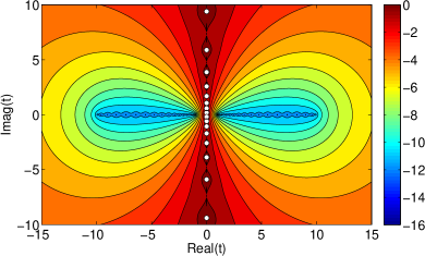
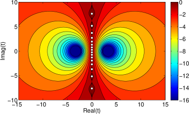
Figure 1: Error of the Zolotarev rational approximation (left) and the Neuberger rational approximation (right). Both rational approximations are of the form $g_{s}(t)=t\sum_{i=1}^{s}\omega_{i}/(t^{2}-\sigma_{i})$ with $\sigma_{i}<0$. We took $s=10$ in both cases and plotted the contours for $\log_{10}(g_{10}(t)-\operatorname{sign}(t))$. We chose $a=1$ and $b=10$ for the Zolotarev approximation, and $c=1/\sqrt{10}$ for the Neuberger approximation. The white spots on the imaginary axis mark the poles $t=\pm i\sqrt{-\sigma_{i}}$ of the rational approximation that lie in the interval $i[-10,10]$.

In this section we address the issue of how to find good rational approximations to the sign function in the non-Hermitian case.

In the Hermitian case, if we know intervals $[-b,-a]$, $[a,b]$ which contain the (deflated) spectrum of $A$, the sign function of $A$ can be approximated using the Zolotarev best rational approximation, see [28] and, e.g., [29, 6]. Using the Zolotarev approximation on non-Hermitian matrices gives rather poor results, unless all eigenvalues are close to the real axis (see the left plot in Figure 1). A better choice for generic non-Hermitian matrices is the rational approximation originally suggested by Kenney and Laub [30] and used by Neuberger [31, 32] for vanishing chemical potential,

$$\operatorname{sign}(t)\approx g_{s}(ct)\,,\mbox{ where }g_{s}(t)=\frac{(t+1)^{2s}-(t-1)^{2s}}{(t+1)^{2s}+(t-1)^{2s}}\,.$$ (29)

Note that $g_{s}(t)=g_{s}(1/t)$, and $g_{s}(t)=\tanh\left(2s\;\text{atanh}\,t\right)$ for $|t|<1$. The partial fraction expansion of $g_{s}$ is known to be

$$g_{s}(t)=t\sum_{i=1}^{s}\frac{\omega_{i}}{t^{2}-\sigma_{i}}\quad\text{with }\omega_{i}=\frac{1}{s}\cos^{-2}\left(\frac{\pi}{2s}\left(i-\frac{1}{2}\right)\right)\,,\quad\sigma_{i}=-\tan^{2}\left(\frac{\pi}{2s}\left(i-\frac{1}{2}\right)\right)\,,$$ (30)

see [30, 31]. In (29), $c>0$ is a parameter which one chooses to minimize the number of poles $s$ of the partial fraction expansion (30), see [6] and the discussion after Theorem 1 below. Whereas for the Zolotarev approximation the regions of good approximation are concentrated along the real axis, the approximation $g_{s}(t)$ approaches $\operatorname{sign}(t)$ well on circles to the left and right of the imaginary axis, see the right plot in Figure 1. For this reason, the Neuberger approximation is better suited for generic non-Hermitian matrices. All we need is some a priori information on the spectrum from which we can determine an appropriate circle $C$ in the right half-plane, centered on the real axis, such that $C$ together with $-C$ contains all the eigenvalues. We then can compute the degree $s$ of the Neuberger approximation such that the sign function is approximated to a given accuracy on $C\cup-C$.

The following theorem gives the insight necessary for this approach to work.

Theorem 1

For given $s$ and $\epsilon>0$ we have

$$|e_{s}(t)|=|g_{s}(t)-\operatorname{sign}(t)|\leq\epsilon\quad\text{for }t\in C_{s,\epsilon}\text{ or }-t\in C_{s,\epsilon}\,,$$ (31)

where $C_{s,\epsilon}$ is the circle with radius $R=2\delta(\epsilon,s)/[\delta(\epsilon,s)^{2}-1]$ and center $M=[\delta(\epsilon,s)^{2}+1]/[\delta(\epsilon,s)^{2}-1]$, with $\delta(\epsilon,s)=(2/\epsilon+1)^{1/(2s)}$.

Proof. Assume that $t$ is in the right half-plane (the case of $t$ in the left half-plane can be treated in a completely analogous manner). With $z=[(t+1)/(t-1)]^{2s}$ we write $g_{s}(t)=(z-1)/(z+1)$ such that $e_{s}(t)=g_{s}(t)-1=-2/(z+1)$. Therefore $|e_{s}(t)|\leq\epsilon$ if and only if $|z+1|\geq 2/\epsilon$.

Since $|z|-1\leq|z+1|$, a sufficient condition for $|e_{s}(t)|\leq\epsilon$ is $|z|-1\geq 2/\epsilon$, which is equivalent to

$$\left|\frac{t+1}{t-1}\right|\geq\left(\frac{2}{\epsilon}+1\right)^{1/(2s)}=\delta(\epsilon,s)\,.$$ (32)

Let $t=x+iy$ be on the circle $C_{s,\epsilon}$, i.e., $(x-M)^{2}+y^{2}=R^{2}$. Then

$$\left|\frac{t+1}{t-1}\right|^{2} =\frac{(x+1)^{2}+y^{2}}{(x-1)^{2}+y^{2}}$$

$$=\frac{(x+1)^{2}+R^{2}-(x-M)^{2}}{(x-1)^{2}+R^{2}-(x-M)^{2}}$$

$$=\frac{2x(M+1)+1+R^{2}-M^{2}}{2x(M-1)+1+R^{2}-M^{2}}\,.$$ (33)

In fact we have $1+R^{2}-M^{2}=1+(R-M)(R+M)=1-\frac{\delta(\epsilon,s)-1}{\delta(\epsilon,s)+1}\cdot\frac{\delta(\epsilon,s)+1}{\delta(\epsilon,s)-1}=0$ and thus

$$\left|\frac{1+t}{1-t}\right|^{2}=\frac{M+1}{M-1}=\frac{\frac{\delta(\epsilon,s)^{2}+1}{\delta(\epsilon,s)^{2}-1}+1}{\frac{\delta(\epsilon,s)^{2}+1}{\delta(\epsilon,s)^{2}-1}-1}=\delta(\epsilon,s)^{2}\,.$$ (34)

So we have shown that $|e_{s}(t)|\leq\epsilon$ on the boundary of the circle $C_{s,\epsilon}$, and by the maximum modulus principle this also holds for $t$ inside the circle. $\Box$

The parameter $c$ in (29) can now be used in order to optimize the number of poles for a given target accuracy $\epsilon$ if the spectrum of the operator is known to be contained in the union of two circles $C(m,r)\cup C(-m,r)$, where $C(m,r)$ is the circle $\{|z-m|\leq r\}$ and $m$ is real, $0<r<m$. For symmetry reasons it is again sufficient to discuss only the circle in the right half-plane, $C(m,r)$. Note that $s$ is a positive integer. Restricting the function $g_{s}(t)$ to real arguments, we see that it is positive on $(0,\infty)$, monotonically increasing on $t\in(0,1]$, and that $g_{s}(t)=g_{s}(1/t)$ as well as $g_{s}(1)=1$. The maximum error $e_{\max}=\max_{t\in[m-r,m+r]}|1-g_{s}(ct)|$ is therefore smallest if $c$ is chosen such that the scaled interval $[c(m-r),c(m+r)]$ is of the form $[1/d,d]$. This is the case for $c=((m+r)(m-r))^{-1/2}$ with $d=((m+r)/(m-r))^{1/2}$, see also [6]. For this choice of $c$ we see that $t$ is in $C(m,r)$ if and only if $ct$ is in $C(M,R)$ with $M=\frac{d^{2}+1}{2d}$ and $R=\frac{d^{2}-1}{2d}$. But $C(M,R)$ is precisely of the form that was considered in Theorem 1 with $\delta(\epsilon,s)=\frac{d+1}{d-1}$. Therefore, if we want the error $|g_{s}(ct)-1|$ to be smaller than $\epsilon$ for $t\in C(m,r)$, Theorem 1 tells us that it is sufficient to require $\frac{d+1}{d-1}=\delta(\epsilon,s)=(2/\epsilon+1)^{1/(2s)}$. Solving for $s$ we see that this precision is obtained if the number $s$ of poles satisfies

$$s\geq\frac{\log\left(\frac{\epsilon}{\epsilon+2}\right)}{2\cdot\log\left(\frac{d-1}{d+1}\right)}.$$ (35)

6 Numerical results

This section contains the results of several numerical experiments comparing some of the methods developed in this paper. We only present results for Algorithms 1 and 4 since the results for Algorithms 2 and 3 are very similar to those of Algorithm 1 [20]. Algorithms 1 and 4 as described in Section 4 were applied to compute $\operatorname{sign}(H_{W})b$, where $H_{W}=\gamma_{5}D_{W}(\mu)$ is the “Hermitian” Wilson Dirac operator at nonzero chemical potential and $b=\left(1,\dots,1\right)$ for generic QCD gauge field configurations on lattices with sizes $4^{4},6^{4},8^{4}$, and $10^{4}$. The lattice parameters are $\beta=5.1$, $m_{W}=-2$, $m_{q}=0$, and $\mu=0.3$, see [5] for the notation.

In Algorithm 1 one has to decide which rational approximation to use. This decision should be made depending on the spectrum of $A$. Even though in lattice QCD the eigenvalues do not move far away from the real axis for reasonable values of $\mu$, we adopted a conservative strategy and used the Neuberger approximation in our numerical experiments. As we discussed at the end of section 5, in order to use a Neuberger rational approximation we have to determine circles $C(m,r)$ and $C(-m,r)$ which should contain all the eigenvalues (except the ones that have been deflated). Of course, we cannot precompute the whole spectrum, so we have to rely on a reasonable heuristics. From the deflation process we know a parameter $\alpha>0$ such that all non-deflated eigenvalues have modulus larger than $\alpha$. We also precomputed the eigenvalue which is largest in modulus with value $\beta>0$. The heuristics, which is confirmed by additional numerical experiments, is to assume that for reasonable values of $\mu$ all eigenvalues are contained in the two circles centered on the real line and intersecting it at the points $\alpha$, $\beta$ and $-\alpha$, $-\beta$, respectively. This gives $m=(\alpha+\beta)/2$ and $r=(\beta-\alpha)/2$. The number of poles to use is now given by (35) together with the corresponding (scaled) Neuberger approximation. Note that this approach is quite defensive since it allows eigenvalues to deviate substantially from the real axis if their real parts are not close to $\alpha$, $\beta$, $-\alpha$ or $-\beta$. For larger lattice volumes and $\mu$ relatively small we observed that the Zolotarev approximation based on the intervals $[-\beta,-\alpha]$ and $[\alpha,\beta]$ can be an interesting alternative, since the spectrum deviates only marginally from the real axis. Using Zolotarev instead of Neuberger would reduce the computational cost for the restarted FOM method since the number of poles $s$ would be reduced (since this moves the smallest shifts away from the origin, it also leads to a reduction in $k_{\text{tot}}$). However, as mentioned above, we only used the more conservative Neuberger approximation.

In Algorithm 1 one also has to decide when the iteration to solve any of the linear systems is considered to be converged. We require the norms of the residuals to be less than $\epsilon$, with $\epsilon$ the target accuracy of the rational approximation defined in Eq. (31). This gives an upper bound of $\approx 2\epsilon$ on the total error. In our experiments we observed that the total error (as defined in the next paragraph) was smaller (as small as $0.1\epsilon$), which is natural since most of the eigenvalues are in the interior of the circles $C(m,r)$ and $C(-m,r)$, where the approximation works better than at the boundary.

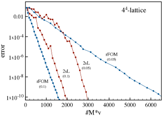
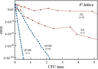
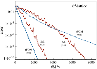
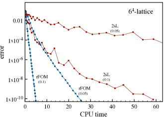
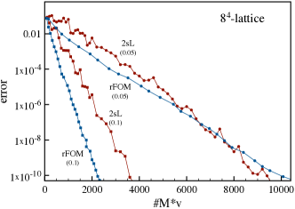
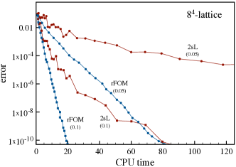
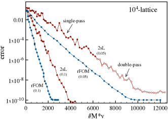
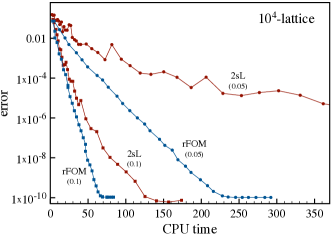
Figure 2: Comparison of the accuracy of the restarted FOM-LR algorithm (rFOM) and the direct two-sided Lanczos-LR method (2sL) as a function of the number of matrix-vector multiplications (left) and the CPU time in seconds (right) for a $4^{4}$ (row 1), $6^{4}$ (row 2), $8^{4}$ (row 3), and $10^{4}$ (row 4) lattice configuration. Each plot shows data for two different deflation gaps, given in parentheses. The restart size used in the restarted FOM-LR algorithm is ${k_{\text{max}}}=30$ for the $4^{4}$ lattice, ${k_{\text{max}}}=40$ for the $6^{4}$ and $8^{4}$ lattices and ${k_{\text{max}}}=50$ for the $10^{4}$ lattice.

We now turn to the question of how to determine the accuracy of the approximations to the sign function in our numerical tests. The exact error cannot be determined because the computational cost to evaluate $\operatorname{sign}(A)b$ exactly by a direct method is too large if $A$ is large. To obtain an estimate for the error, we compute $\operatorname{sign}(A)^{2}b$ (by applying $\operatorname{sign}(A)$ twice in succession), which should equal $b$ if the approximation to the sign function were exact, and then take $\frac{1}{2}||\operatorname{sign}(A)^{2}b-b||/||b||$ as a measure for the error (or accuracy). Of course, in production runs one would check the quality of the approximation only occasionally.

In Figure 2 we compare the results of the restarted FOM-LR approximation with those of the direct two-sided Lanczos-LR method for various lattice sizes: $4^{4}$ ($n=3,072$), $6^{4}$ ($n=15,552$), $8^{4}$ ($n=49,152$), and $10^{4}$ ($n=120,000$), and for two different deflation gaps, i.e., the modulus of the smallest non-deflated eigenvalue.^, The accuracy is shown as a function of the number of matrix-vector multiplications (left) and as a function of the CPU time on a 2.4 GHz Intel Core 2 with 8 GB of memory (right). Although the number of matrix-vector multiplications is often used to compare the efficiency of different iterative methods, it is not the best measure of the efficiency since it only includes the first term in Eqs. (26) and (28), respectively. The total run time is a better measure since it includes the other terms as well. Depending on the parameters actually used, some of these terms can be dominant or negligible. E.g., the $\mathcal{O}(k^{3})$ term in the two-sided-Lanczos-LR method becomes dominant when the Krylov subspace grows. Another example are the $\mathcal{O}(mn)$ terms in both algorithms, which reflect the cost of using the deflated eigenvectors and which could be neglected in all cases we considered. Note that for the two smaller lattices a larger fraction of the problem fits in cache, which leads to a reduction of the run time.

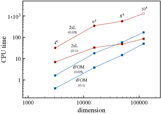
Figure 3: Run time (in seconds) for the restarted FOM-LR algorithm and the direct two-sided Lanczos-LR method as a function of the matrix size to achieve an accuracy of $10^{-8}$. The run time does not include the cost of deflation. The deflation gaps are given in parentheses, and the restart sizes are the same as in Figure 2. The data point for 2sL(0.05) on a $10^{4}$ lattice (open circle) was computed in double-pass for memory reasons.

In Figure 3 we show how the efficiency of both methods scales with the volume. This figure should be interpreted with care. Since we used a constant deflation gap we expect the number of iterations ($k_{\text{tot}}$ resp. $k$) to be approximately constant. This would result in a contribution to the execution time which is linearly dependent on the volume, for both methods. However, there are several effects which obscure this linear dependence. For example, in the restarted FOM there is a dependence on $k_{\max}$. In the direct two-sided Lanczos method the ${\cal O}(k^{3})$ cost to compute $f(H_{k})$ dominates for small volumes. In addition, there are the cache effects already mentioned.

The restarted FOM-LR method contains three tunable parameters: the deflation gap $m$, the number $s$ of poles in the partial fraction expansion and the restart size $k_{\text{max}}$, i.e., the maximal size of the Krylov subspace before restarting. Figure 4 shows the effect of the restart size on the CPU time used by the restarted FOM-LR method. Clearly, there is an optimal size which should be determined before performing production runs. The number of poles in the partial fraction expansion is chosen adequately to achieve the desired accuracy, and strongly depends on the deflation gap. In our numerical results the number of poles varied between 8 and 70.

             

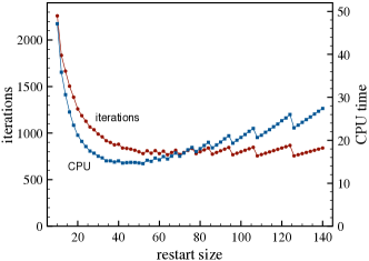
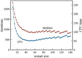
Figure 4: Dependence of the number of iterations and run time (in seconds) on the restart size for the restarted FOM-LR method to achieve an accuracy of $10^{-8}$ for an $8^{4}$ configuration (left) and a $10^{4}$ configuration (right). The deflation gap is 0.1 in both cases.

7 Conclusions

At nonzero chemical potential, the overlap Dirac operator contains the sign function of the Wilson operator $H_{W}=\gamma_{5}D_{W}$, which is non-Hermitian. The by far most expensive part when applying the overlap Dirac operator to a field vector $b$ — the standard step in any iterative solver for the overlap Dirac operator — is the computation of the action of $\operatorname{sign}(H_{W})$ on $b$. As a step towards developing computationally feasible methods for the dynamical simulation of overlap fermions at nonzero chemical potential, we proposed in this paper several short-recurrence Krylov subspace methods to efficiently compute $\operatorname{sign}(H_{W})b$.

One class of methods is based on restarts of the Arnoldi process and requires a precise rational approximation for the sign function on the (complex) spectrum of the Wilson operator. This means that we need to have information on the location of the spectrum in the complex plane and that we have to adapt the number of poles in the rational approximation accordingly. The storage requirements for these methods depend on the restart value, a parameter which has to be tuned to be optimal, and the number of poles in the rational approximation. Storage does not depend on the number of iterations to be performed.

The other class of methods relies on the two-sided Lanczos process. We can use a rational function approximation, in which case the comments made in the previous paragraph apply as well, except that there is no restart. Alternatively, the sign function can be evaluated directly. In that case, if a two-pass strategy is used, the storage requirements are minimal; otherwise storage increases linearly with the number of iterations. No a priori knowledge on the spectrum is required. If the number of iterations to be performed gets large, the work spent in evaluating the sign function of the projected operator, which is represented by a tridiagonal matrix, becomes decisive in terms of computational cost. Therefore, the methods based on a rational function approximation were faster in the numerical experiments that we performed on lattices with sizes ranging from $4^{4}$ to $10^{4}$. However, fast methods are currently being developed to compute the sign of the projected tridiagonal matrix, which will speed up the direct two-sided Lanczos method substantially [26].

For both classes of methods the deflation of critical eigenvalues is an important ingredient towards efficiency. We showed that LR deflation is to be preferred to Schur deflation.

References

- [1] R. Narayanan, H. Neuberger, A construction of lattice chiral gauge theories, Nucl. Phys. B443 (1995) 305–385. arXiv:hep-th/9411108.
- [2] H. Neuberger, Exactly massless quarks on the lattice, Phys. Lett. B417 (1998) 141–144. arXiv:hep-lat/9707022.
- [3] P. H. Ginsparg, K. G. Wilson, A remnant of chiral symmetry on the lattice, Phys. Rev. D25 (1982) 2649.
- [4] M. Lüscher, Exact chiral symmetry on the lattice and the Ginsparg-Wilson relation, Phys. Lett. B428 (1998) 342–345. arXiv:hep-lat/9802011.
- [5] J. C. R. Bloch, T. Wettig, Overlap Dirac operator at nonzero chemical potential and random matrix theory, Phys. Rev. Lett. 97 (2006) 012003. arXiv:hep-lat/0604020.
- [6] J. van den Eshof, A. Frommer, T. Lippert, K. Schilling, H. A. van der Vorst, Numerical methods for the QCD overlap operator. I: Sign-function and error bounds, Comput. Phys. Commun. 146 (2002) 203–224. arXiv:hep-lat/0202025.
- [7] J. C. R. Bloch, T. Wettig, Domain-wall and overlap fermions at nonzero quark chemical potential, Phys. Rev. D76 (2007) 114511. arXiv:0709.4630.
- [8] J. C. R. Bloch, A. Frommer, B. Lang, T. Wettig, An iterative method to compute the sign function of a non- Hermitian matrix and its application to the overlap Dirac operator at nonzero chemical potential, Comput. Phys. Commun. 177 (2007) 933–943. arXiv:0704.3486.
- [9] N. J. Higham, Functions of Matrices: Theory and Computation, Society for Industrial and Applied Mathematics, 2008.
- [10] A. Frommer, V. Simoncini, Matrix Functions, Vol. 13 of Mathematics in Industry, Springer, Heidelberg, 2008, Ch. 3, pp. 275–303.
- [11] H. van der Vorst, An iterative solution method for solving , using Krylov subspace information obtained for the symmetric positive definite matrix A., J. Comput. Appl. Math. 18 (1987) 249–263.
- [12] J. C. R. Bloch, T. Wettig, A. Frommer, B. Lang, An iterative method to compute the overlap Dirac operator at nonzero chemical potential, PoS LAT2007 (2007) 169. arXiv:0710.0341.
- [13] M. Eiermann, O. Ernst, A restarted Krylov subspace method for the evaluation of matrix functions, SIAM J. Numer. Anal. 44 (2006) 2481–2504.
- [14] B. N. Parlett, A new look at the Lanczos algorithm for solving symmetric systems of linear equations, Linear Algebra Appl. 29 (1980) 323–346.
- [15] C. C. Paige, B. N. Parlett, H. A. van der Vorst, Approximate solutions and eigenvalue bounds from Krylov subspaces, Numer. Linear Algebra Appl. 2 (2) (1995) 115–134.
- [16] Y. Saad, Iterative Methods for Sparse Linear Systems, 2nd Edition, SIAM, Philadelphia, 2003.
- [17] A. Frommer, BiCGStab(l) for families of shifted linear systems, Computing 70 (2) (2003) 87–109.
- [18] V. Simoncini, Restarted full orthogonalization method for shifted linear systems, BIT Numerical Mathematics 43 (2003) 459–466.
- [19] A. Frommer, U. Glässner, Restarted GMRES for shifted linear systems, SIAM J. Sci. Comput. 19 (1998) 15–26.
- [20] K. Schäfer, Krylov subspace methods for shifted unitary matrices and eigenvalue deflation applied to the Neuberger Operator and the matrix sign function, Ph.D. thesis, University of Wuppertal (2008).
- [21] J. C. R. Bloch, T. Breu, T. Wettig, Comparing iterative methods to compute the overlap Dirac operator at nonzero chemical potential, PoS LATTICE2008 (2008) 027. arXiv:0810.4228.
- [22] B. Jegerlehner, Krylov space solvers for shifted linear systems (1996). arXiv:hep-lat/9612014.
- [23] H. A. van der Vorst, BI-CGSTAB: a fast and smoothly converging variant of BI-CG for the solution of nonsymmetric linear systems, SIAM J. Sci. Stat. Comput. 13 (2) (1992) 631–644.
- [24] R. W. Freund, N. M. Nachtigal, QMR: a Quasi-Minimal Residual Method for Non-Hermitian Linear Systems, Numer. Math. 60 (1991) 315–339.
- [25] R. W. Freund, Solution of Shifted Linear Systems by Quasi-Minimal Residual Iterations, in: L. Reichel, A. Ruttan, R. S. Varga (Eds.), Numerical Linear Algebra, W. de Gruyter, 1993, pp. 101–121.
- [26] J. C. R. Bloch, S. Heybrock, A nested Krylov subspace method to compute the sign function of large complex matrices (2009). arXiv:0912.4457.
- [27] G. H. Golub, C. F. van Loan, Matrix Computations, 3rd Edition, Johns Hopkins University Press, 1996.
- [28] E. I. Zolotarev, Application of elliptic functions to the question of functions deviating least and most from zero, Zap. Imp. Akad. Nauk. St. Petersburg 30 (1877) .
- [29] D. Ingerman, V. Druskin, L. Knizhnerman, Optimal finite difference grids and rational approximations of the square root. I. Elliptic problems, Comm. Pure Appl. Math. 53 (8) (2000) 1039–1066.
- [30] C. Kenney, A. Laub, A hyperbolic tangent identity and the geometry of Padé sign function iterations, Numer. Algorithms 7 (2-4) (1994) 111–128.
- [31] H. Neuberger, A practical implementation of the overlap Dirac operator, Phys. Rev. Lett. 81 (1998) 4060–4062. arXiv:hep-lat/9806025.
- [32] H. Neuberger, The overlap Dirac operator, in: A. Frommer, T. Lippert, B. Medeke, K. Schilling (Eds.), Numerical challenges in Lattice Quantum Chromodynamics, Springer Berlin, 2000, pp. 1–17. arXiv:hep-lat/9910040.