NEW TESTS FOR DISRUPTION MECHANISMS OF STAR CLUSTERS: METHODS AND APPLICATION TO THE ANTENNAE GALAXIES

Abstract

We present new tests for disruption mechanisms of star clusters based on the bivariate mass-age distribution $g(M,\tau)$. In particular, we derive formulae for $g(M,\tau)$ for two idealized models in which the rate of disruption depends on the masses of the clusters and one in which it does not. We then compare these models with our Hubble Space Telescope observations of star clusters in the Antennae galaxies over the mass-age domain in which we can readily distinguish clusters from individual stars: $\tau\lesssim 10^{7}(M/10^{4}M_{\odot})^{1.3}$ yr. We find that the models with mass-dependent disruption are poor fits to the data, even with complete freedom to adjust several parameters, while the model with mass-independent disruption is a good fit. The successful model has the simple form $g(M,\tau)\propto M^{-2}\tau^{-1}$, with power-law mass and age distributions, $dN/dM\propto M^{-2}$ and $dN/d\tau\propto\tau^{-1}$. The predicted luminosity function is also a power law, $dN/dL\propto L^{-2}$, in good agreement with our observations of the Antennae clusters. The similarity of the mass functions of star clusters and molecular clouds indicates that the efficiency of star formation in the clouds is roughly independent of their masses. The age distribution of the massive young clusters is plausibly explained by the following combination of disruption mechanisms: (1) removal of interstellar material by stellar feedback, $\tau\lesssim 10^{7}$ yr; (2) continued stellar mass loss, $10^{7}{\rm yr}\lesssim\tau\lesssim 10^{8}{\rm yr}$; (3), tidal disturbances by passing molecular clouds, $\tau\gtrsim 10^{8}$ yr. None of these processes is expected to have a strong dependence on mass, consistent with our observations of the Antennae clusters. We speculate that this simple picture also applies—at least approximately—to the clusters in many other galaxies.

1 INTRODUCTION

Star clusters are born in molecular clouds and are then dispersed into the surrounding stellar field by a variety of processes operating on different timescales, including the removal of interstellar material by stellar feedback, continued stellar mass loss, tidal disturbances by passing molecular clouds, gravitational shocks during rapid passages near the galactic bulge or through the galactic disk, orbital decay into the galactic center caused by dynamical friction, and stellar escape driven by internal two-body relaxation. Signatures of these processes are encoded in the mass function, $\psi(M)\propto dN/dM$, and the age distribution, $\chi(\tau)\propto dN/d\tau$, for a population of clusters in a particular galaxy. A more informative, but less familiar statistic is the bivariate distribution of masses and ages, $g(M,\tau)\propto\partial^{2}N/\partial{M}\partial{\tau}$. The key feature of $g(M,\tau)$ is that it includes correlations between $M$ and $\tau$, information that is absent from the univariate distributions $\psi(M)$ and $\chi(\tau)$. Thus, with the help of $g(M,\tau)$, we can answer questions such as whether low-mass clusters are disrupted faster than, or at the same rate as, high-mass clusters. In this paper, we derive formulae for $g(M,\tau)$ for the first time for several different models for the disruption of clusters, and we then compare these formulae with our Hubble Space Telescope (HST) observations of clusters in the Antennae galaxies. In a companion paper, we present similar comparisons for the clusters in the Large and Small Magellanic Clouds (LMC and SMC; Chandar et al. 2009, hereafter CFW09).

We have focused on the star clusters in the Antennae galaxies for several reasons. First, the population of clusters is large, $N\approx 2300$ brighter than $M_{V}=-9$, ample for statistical studies. Second, many of the bright young clusters have masses in the range of old globular clusters, $10^{4}\lesssim M/M_{\odot}\lesssim 10^{6}$, suggesting that the former may simply be younger versions of the latter. Third, because the Antennae are currently in the throes of a major merger, they give us a close-up, internal view of events and processes that were more common in galaxies in the past, during their hierarchical formation. Fourth, the Antennae have been mapped at almost every wavelength available to astronomers, from radio to X-rays, providing a more detailed picture of their stellar and interstellar contents than for almost any other galaxy outside the Local Group.

In our previous studies of the clusters in the Antennae, we found that the mass and age distributions could be approximated by power laws: $\psi(M)\propto M^{\beta}$ with $\beta\approx-2$ (Zhang & Fall 1999, hereafter ZF99) and $\chi(\tau)\propto\tau^{\gamma}$ with $\gamma\approx-1$ (Fall et al. 2005, hereafter FCW05). In these studies, we also found that the shapes of $\psi(M)$ and $\chi(\tau)$ are approximately independent of the age and mass limits, respectively, of the samples used to determine them. These findings suggest that the bivariate mass-age distribution can be approximated simply by the product of the univariate distributions:

$$g(M,\tau)\propto\psi(M)\chi(\tau)\propto M^{\beta}\tau^{\gamma}$$ (1)

$${\rm for}\,\,\,\,\,\,\,\,\,\tau\lesssim 10^{7}(M/10^{4}M_{\odot})^{1.3}\,{\rm yr}.$$ (2)

The second expression above indicates the approximate domain of validity of the first, the condition that objects in the sample be brighter than the most luminous individual stars ($L_{V}\gtrsim 3\times 10^{5}L_{\odot}$). In this model, clusters form with a power-law initial mass function and are then disrupted at rates that are independent of their masses. We have already explored some of the consequences of equation (1) in two recent papers (Fall 2006; Whitmore et al. 2007, hereafter WCF07). In this paper, we make further tests of this model, and we also compare our HST observations of the Antennae clusters with two models in which clusters of different masses are disrupted at different rates.

The age distribution for a population of star clusters reflects, in principle, a combination of both formation and disruption rates. We interpret the decline of $\chi(\tau)$ primarily as the result of disruption rather than formation for the following reasons. First, the age distribution has a sharp peak at the present time, $\tau=0$, and a small width, characterized by the median age $\tau\sim 10^{7}$ yr. This requires either rapid disruption at an arbitrary time (now) or rapid formation at a special time (now), the former being much more likely a priori than the latter. Of course, the Antennae galaxies are presently merging, which has almost certainly boosted the formation rates of stars and clusters, but this occurs more slowly, on the orbital timescale of the galaxies, $\tau\sim{\rm few}\times 10^{8}$ yr. In the simulations of merging galaxies by Mihos et al. (1993), including the Antennae, for example, the star formation rate varies by factors of only a few or less in the past $10^{8}$ yr, whereas the observed age distribution of the clusters drops by nearly 2 orders of magnitude in this interval of time. The second reason we interpret the decline of $\chi(\tau)$ in terms of disruption is that it has the same shape, including the sharp peak at $\tau=0$, in large regions separated by distances of order 10 kpc within the Antennae galaxies (Whitmore 2004; WCF07). There is no physical mechanism that could synchronize a burst of cluster formation this precisely at these separations; the communication time is $\tau\sim 10^{9}$ yr for a signal traveling at the typical random velocity in the interstellar medium (ISM; $v\sim 10$ km s^-1) and $\tau\sim 10^{8}$ yr for one traveling at the highest bulk velocity ($v\sim 100$ km s^-1). Thus, we conclude that the observed decline in the age distribution is caused mainly by disruption, at least for $\tau\lesssim\mbox{few}\times 10^{8}$ yr.

We have speculated that equation (1) for $g(M,\tau)$ may also describe—approximately—the cluster populations in other galaxies (Fall 2006; WCF07). If this picture turns out to be generally valid, it will mean that star clusters form and evolve in much the same way in different galaxies, the primary variable being an overall scale factor proportional to the total number of clusters and hence to their average formation rate. We define a cluster here to be any concentrated aggregate of stars with a density much higher than that of the surrounding stellar field, whether or not it is gravitationally bound, since this is virtually impossible to determine from the available observations, especially for clusters younger than about 10 internal crossing times. Most, if not all, stars form in clusters (as just defined) and most clusters then dissolve into the stellar field. We find it intriguing that this whole complex process might be represented approximately by a simple “recipe” such as equation (1).

There are a few other hints that point toward this model: (1) The same mass and age distributions, $\psi(M)\propto M^{-2}$ and $\chi(\tau)\propto\tau^{-1}$, are found for clusters with $M\lesssim 10^{3}M_{\odot}$ and $\tau\lesssim 3\times 10^{8}$ yr in the solar neighborhood (Lada & Lada 2003). (2) The luminosities of the brightest clusters in different galaxies scale approximately with the size of the population in the way expected from equation (1) (Larsen 2002; Whitmore 2003; WCF07). (3) The mass spectrum of molecular clouds, from which the clusters form, appears to be similar in different galaxies (Blitz et al. 2007). (4) The most important early disruption processes, removal of ISM by stellar feedback and continued stellar mass loss, are independent of the properties of the host galaxy (except possibly its metallicity and stellar initial mass function (IMF)). Of course, a definitive conclusion about the generality of equation (1) will require more detailed studies, such as that presented here for the Antennae, of the cluster populations in several other galaxies. We have recently made a start on this with the LMC and SMC (CFW09). Our main purpose in this paper is to present some of the interpretive tools needed for such studies.

The plan for the remainder of this paper is the following: In §2, we present analytic formulae for $g(M,\tau)$ for two models with mass-dependent disruption and the model already mentioned with mass-independent disruption. In §3, we describe our HST observations of the Antennae clusters and compare these with the models presented in the previous section. We also derive the luminosity function of the Antennae clusters and show how this is related to the mass function through $g(M,\tau)$. In §4, we discuss the physical processes most likely responsible for the formation and disruption of clusters and how these processes affect the mass and age distributions. This interpretative section presents our current understanding of the entire life cycles of star clusters. In §5, we summarize our main results and their broader implications. The paper also includes two appendices. The first (A) discusses some related work on the mass and luminosity functions of the Antennae clusters by Mengel et al. (2005) and by Anders et al. (2007) respectively, while the second (B) presents some specialized formulae needed in §3.

2 MODELS

The basic element of a statistical description of a population of star clusters is the multivariate distribution of all the important properties of the clusters, such as their luminosities, masses, ages, effective radii, internal concentrations, stellar contents, and so forth. For a population of clusters more distant than $\sim 10$ Mpc, however, many clusters are poorly resolved or not resolved at all, and the list of available properties shrinks to just three: luminosities, masses, and ages, of which only two are independent if the stellar IMF is assumed to be universal, as it almost always is in practice. With these thoughts in mind, we focus here on the bivariate distribution $g(M,\tau)$, defined such that $g(M,\tau)dMd\tau$ is the number of clusters with masses between $M$ and $M+dM$ and ages between $\tau$ and $\tau+d\tau$. This distribution can be estimated from fits of stellar population models to photometry in several bands of the clusters in a large sample, as we describe in the next section.

The goal of this section is to relate $g(M,\tau)$ to information about the formation and disruption of the clusters. This is done most easily with the help of a few auxiliary functions. We define another distribution $f(M_{0},\tau)$ such that $f(M_{0},\tau)dM_{0}d\tau$ is the number of clusters born with initial masses between $M_{0}$ and $M_{0}+dM_{0}$ at times in the past between $\tau$ and $\tau+d\tau$. Furthermore, we assume that the current mass $M(M_{0},\tau)$ of a cluster with an initial mass $M_{0}$ and the inverse relation $M_{0}(M,\tau)$ are known functions of the age $\tau$. Then $f$ and $g$ are related by the continuity equation in the form

$$g(M,\tau)=f[M_{0}(M,\tau),\tau](\partial{M_{0}}/\partial{M})_{\tau}.$$ (3)

This generalizes equation (2) of Fall & Zhang (2001) from an instantaneous burst to an arbitrary history of cluster formation. In equation (3) here, all information about formation is encoded in $f(M_{0},\tau)$, while all information about disruption is encoded in $M(M_{0},\tau)$ and hence in the difference between $f$ and $g$. In fact, these distributions are equal only if clusters are never disrupted (i.e., $M=M_{0}$ for all $\tau$).

We can exploit equation (3) in either of two ways. If we knew everything about the disruption mechanisms (likely more than one) and hence the precise form of $M(M_{0},\tau)$, we could use the empirical determination of $g(M,\tau)$ together with equation (3) to infer $f(M_{0},\tau)$. In practice, however, we must work in the other direction: make reasonable assumptions about $f(M_{0},\tau)$, adopt a specific model for $M(M_{0},\tau)$, compute $g(M,\tau)$ from equation (3), and compare this with the corresponding empirical distribution to see if the model is acceptable or must be rejected. In this spirit, we assume that clusters form with the following initial mass-age distribution:

$$f(M_{0},\tau)=C(\tau)(M_{0}/M_{*})^{\beta}.$$ (4)

Here $C(\tau)$, with units of [mass]^-1 [time]^-1, specifies the formation rate of clusters at an age $\tau$, while $M_{*}$ is a fiducial mass, usually taken to be $10^{4}~{}M_{\odot}$. Our assumption that the initial mass function is a power law is justified by our previous results and those presented in the next section of this paper. In all our detailed comparisons with observations, we assume for simplicity that the formation rate $C(\tau)$ in equation (4) is constant. For the reasons discussed in the Introduction, this should be a good approximation for the Antennae clusters younger than a $\mbox{few}\times 10^{8}$ yr. It is worth noting here, however, that the mathematical formulae for $g(M,\tau)$ presented in this section [equations (6), (12), and (13) below] are equally valid with a variable formation rate, even one as extreme as an instantaneous burst, with $C(\tau)\propto\delta(\tau-\tau_{0})$. We also note that, although $f(M_{0},\tau)$ is a separable function of $M_{0}$ and $\tau$ (by assumption), $g(M,\tau)$ will generally include correlations between $M$ and $\tau$, except in the special case in which $M/M_{0}$ is a function only of $\tau$.

In the remainder of this section, we present the mass-age distribution $g(M,\tau)$ for three simple, illustrative models for the disruption of clusters. In this context, it is important to bear in mind that several processes probably operate together to disrupt the clusters, with different combinations predominating at different ages over the lifetimes of the clusters. Thus, we cannot expect the most successful model to display the signature of any single process operating in isolation. The massive young clusters in our sample are probably disrupted first by the removal of residual interstellar material driven by early stellar feedback (photoionization, radiation pressure, stellar winds, and supernovae), then by continued mass loss from the stars themselves through stellar winds and other ejecta, and then possibly by the escape of stars driven by tidal disturbances of passing structures such as molecular clouds and/or spiral arms. The three models we consider have simple functional forms but several adjustable parameters to accommodate this likely complexity. We note here that the clusters in our sample are all too massive and too young to have lost a significant fraction of their mass as the result of stellar escape driven by internal two-body relaxation, the primary long-term disruptive process for clusters and one that certainly depends on mass (see §4.3 below).

Model 1: Sudden Mass-Dependent Disruption. In this case, we assume clusters retain all of their initial mass until they are destroyed suddenly and completely at an age $\tau_{d}(M_{0})$:

$$M(\tau)=\left\{\begin{array}[]{ll}M_{0}&\mbox{for $\tau\leq\tau_{d}(M_{0})$}\\ 0&\mbox{otherwise.}\end{array}\right.$$ (5)

The corresponding mass-age distribution, from equations (3), (4), and (5), is

$$g(M,\tau)=\left\{\begin{array}[]{ll}C(M/M_{*})^{\beta}&\mbox{for $\tau\leq\tau_{d}(M)$}\\ 0&\mbox{otherwise.}\end{array}\right.$$ (6)

These equations are valid for any dependence of $\tau_{d}(M_{0})$ on $M_{0}$. Boutloukos & Lamers (2003) have proposed a specific version of this model with a power-law dependence on mass:

$$\tau_{d}(M_{0})=\tau_{*}(M_{0}/M_{*})^{k}.$$ (7)

The discontinuous evolution posited by this model is clearly an oversimplification. Boutloukos & Lamers (2003) claim that Model 1 does, nevertheless, reveal the correct mass dependence of disruption when it is compared with observations. They find the same exponent $k\approx 0.6$ but very different disruption timescales $\tau_{*}$ for the cluster populations in several galaxies. We are skeptical of these claims for reasons we explain in detail in §3 and §4 (see also WCF07).

Model 2: Gradual Mass-Dependent Disruption. In this case, we assume clusters lose mass gradually according to the equations

$$dM/d\tau=-M/\tau_{d}(M),$$ (8)

$$\tau_{d}(M)=\tau_{*}(M/M_{*})^{k}.$$ (9)

The similarity between the disruption timescales $\tau_{d}(M_{0})$ and $\tau_{d}(M)$ in equations (7) and (9) makes Model 2 an analog of Model 1 but with continuous evolution (as noted also by Boutloukos & Lamers 2003). It seems reasonable to suppose that the gradual evolution posited by Model 2 would make it more realistic and hence a better match to the observations than Model 1. Indeed, Model 2 has known physical justifications in two special cases, both of which apply to tidally limited clusters (with constant mean density). For $k=0$, it describes the disruption of clusters by external gravitational shocks, while for $k=1$, it describes the disruption of clusters by internal two-body relaxation (Spitzer 1987). The first of these is potentially relevant to intermediate-age clusters, while the second is certainly relevant to old clusters, as we discuss in detail in §4.

The solutions of equations (8) and (9) are

$$M(\tau)=\left\{\begin{array}[]{ll}M_{0}\left[1-k(M_{0}/M_{*})^{-k}(\tau/\tau_{*})\right]^{1/k}\\ \qquad\mbox{for $k\not=0$}\\ M_{0}\exp(-\tau/\tau_{*})\\ \qquad\mbox{for $k=0$.}\end{array}\right.$$ (10)

Thus, the derivative required in equation (3) is

$$(\partial{M_{0}}/\partial{M})_{\tau}=(M_{0}/M)^{1-k}\hskip 28.45274pt{\rm for}\,\,{\rm all}\,\,k.$$ (11)

Combining equations (3), (4), (10), and (11), we obtain the mass-age distribution

$$g(M,\tau)=\left\{\begin{array}[]{ll}C(M/M_{*})^{\beta}\left[1+k(M/M_{*})^{-k}(\tau/\tau_{*})\right]^{(\beta+1-k)/k}\\ \qquad\mbox{for $k\not=0$}\\ C(M/M_{*})^{\beta}\exp\left[(\beta+1)(\tau/\tau_{*})\right]\\ \qquad\mbox{for $k=0$.}\end{array}\right.$$ (12)

Several features of this equation are noteworthy. For fixed $\tau$ and $k>0$, $g(M,\tau)$ is a double power law with a low-$M$ exponent $k-1$, a gradual bend at the mass given by $\tau\approx\tau_{d}(M)$, and a high-$M$ exponent $\beta$. For fixed $M$ and $k\not=0$, $g(M,\tau)$ is constant for small $\tau$, has a knee at $\tau\approx\tau_{d}(M)$, and is a power law with an exponent $(\beta+1-k)/k$ for large $\tau$. However, for $k=0$, $g(M,\tau)$ is a single power law in $M$ with an exponent $\beta$ for fixed $\tau$, and declines exponentially in $\tau$ with a timescale $-\tau_{*}/(\beta+1)$ (i.e., faster than any power law) for fixed $M$.

Model 3: Gradual Mass-Independent Disruption. In this case, we adopt the mass-age distribution indicated by our earlier studies (ZF99, FCW05, Fall 2006, WCF07), namely

$$g(M,\tau)=C(M/M_{*})^{\beta}(\tau/\tau_{*})^{\gamma}.$$ (13)

This distribution is manifestly separable: $g(M,\tau)\propto\psi(M)\chi(\tau)$, with $\psi(M)\propto(M/M_{*})^{\beta}$ (independent of $\tau$) and $\chi(\tau)\propto(\tau/\tau_{*})^{\gamma}$ (independent of $M$). It has three independent, adjustable parameters: $C$, $\beta$, and $\gamma$. The other parameters, $M_{*}$ and $\tau_{*}$ (which are not independent of $C$, $\beta$, and $\gamma$), merely specify the units in which masses and ages are measured. We can derive equation (13) from equations (3) and (4) with $M(\tau)=M_{0}(\tau/\tau_{*})^{-\gamma/(\beta+1)}$. In this case, the masses of all clusters decline gradually, with the same power law in age. However, this interpretation of equation (13) is not unique. Another possibility is that $g(M,\tau)$ specifies the probability that clusters of mass $M$ survive to an age $\tau$, even if disruption, when it happens, is sudden. The form of $g(M,\tau)$ displayed in equation (13) then implies that the survival probability is independent of mass and declines as a power law in age. Intermediate cases are also possible, with different combinations of age-dependent masses and survival probabilities. Moreover, some clusters may lose only part of their mass (generally in the form of the least bound stars), while others are completely destroyed. We refer to all situations described by equation (13) as gradual mass-independent disruption, irrespective of whether the disruption of individual clusters is gradual or sudden, partial or complete, because it leads to a gradual decline in the number of clusters of each mass with age at a fractional rate independent of mass.

The main justification for Model 3 is that it provides a simple, approximate representation of $g(M,\tau)$ for the massive young clusters in the Antennae galaxies (in the mass-age domain specified by eqn. [2] above). It is likely that the power-law dependence of $g(M,\tau)$ on $M$ reflects the mass function of the molecular clouds in which the clusters formed, and an efficiency of star formation that is nearly independent of the masses of the clouds. The subsequent disruption of many of the young clusters by the removal of their ISM, stellar mass loss, and tidal disturbances also tends to preserve the power-law shape of the mass function. These effects plausibly predominate in the following sequence: (1) removal of ISM, $\tau\lesssim 10^{7}$ yr; (2) stellar mass loss, $10^{7}{\rm yr}\lesssim\tau\lesssim 10^{8}{\rm yr}$; (3) tidal disturbances, $\tau\gtrsim 10^{8}$ yr. This combination of disruptive processes might then account (approximately) for the power-law dependence of $g(M,\tau)$ on $\tau$. Variations in the formation rate could also play some role, although we expect this to be minor, for the reasons discussed in the Introduction. We discuss these issues more fully in §4.

3 OBSERVATIONS AND COMPARISONS WITH MODELS

The goal of this section is to compare the observed mass and age distributions of star clusters in the Antennae with predictions from the three disruption models developed in the previous section. In the next section, we discuss the physical implications of our results for the formation and disruption of the clusters, and in a companion paper we make similar comparisons between models and data for clusters in the Magellanic Clouds (CFW09).

3.1 Observations and Input Data

We have derived the masses and ages of the Antennae clusters from UBVIH$\alpha$ photometry of images taken with the WFPC2 on HST. These images cover nearly all of the main bodies of the Antennae galaxies, omitting only a small region in the northwest and the long tidal tails. Thus, all the results presented in this paper are essentially averages over the two merging galaxies. We describe our procedure in detail in FCW05, including extensive tests of its validity, and the resulting age distributions for mass- and luminosity-limited samples of clusters. Here, we give only a brief summary of our procedure but a more complete set of results, including the bivariate mass-age distribution and the univariate mass and age distributions. The present work also updates the earlier results from ZF99 based on UBVI photometry of the same images, but with masses and ages estimated from two reddening-free $Q$ parameters.

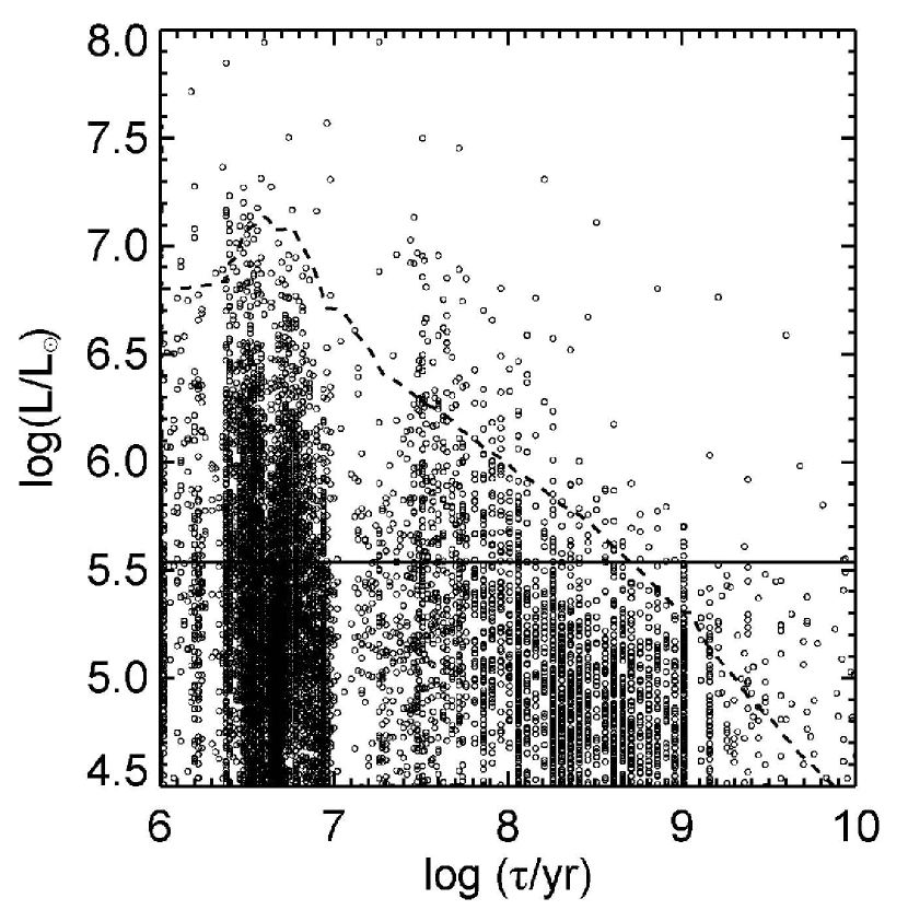
Figure 1: Luminosity-age plane for the Antennae clusters. The luminosities are in the $V$ band and have been corrected for extinction. The dashed diagonal line is the evolutionary track of a model cluster with an initial mass of $M=2\times 10^{5}$ $M_{\odot}$ (Bruzual & Charlot 2003), while the solid horizontal line at $L=3\times 10^{5}$ $L_{\odot}$ is the approximate upper limit for stellar contamination. The vertical gap in the data points just above $\tau=1\times 10^{7}$ yr is an artifact caused by loops in the color tracks of stellar population models during the RSG phase (see the text).

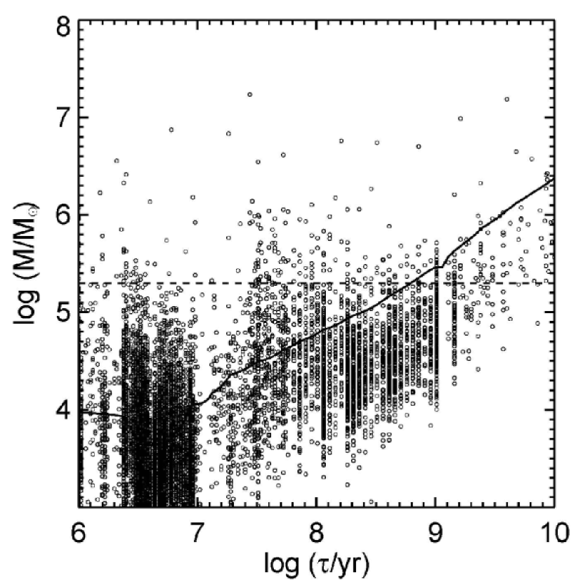
Figure 2: Mass-age plane for the Antennae clusters. This is an alternative, but equivalent, representation of the data plotted in Fig. 1. The lines in the two diagrams are also equivalent: the dashed horizontal one indicates $M=2\times 10^{5}$ $M_{\odot}$, while the solid diagonal one indicates $L=3\times 10^{5}$ $L_{\odot}$, the approximate upper limit for stellar contamination. The vertical gap in the data points just above $\tau=1\times 10^{7}$ yr is an artifact caused by loops in the color tracks of stellar population models during the RSG phase (see the text).

In the present study, we determine the age $\tau$ and extinction $A_{V}$ of each object by performing a minimum $\chi^{2}$ fit between the observed UBVIH$\alpha$ magnitudes and those predicted by stellar population models. We use the Bruzual & Charlot (2003) models with solar metallicity, a Salpeter (1955) IMF with lower and upper cutoffs at 0.1 $M_{\odot}$ and 100 $M_{\odot}$, and the Galactic-type extinction law from Fitzpatrick (1999). Our procedure, which uses measurements in five filters (four colors) simultaneously to estimate two parameters ($\tau$ and $A_{V}$) for each cluster, is thus over-constrained mathematically. The H$\alpha$ flux varies rapidly with age near $\approx 10^{7}$ yr, and is particularly useful in distinguishing clusters younger and older than this. We estimate the masses of the clusters from their total $V$-band luminosity (corrected for extinction) and the age-dependent mass-to-light ratio ($M/L_{V}$) from the stellar population models, assuming a distance of 19.2 Mpc to the Antennae. Figure 1 shows the resulting luminosity-age distribution for all objects, and Figure 2 shows the equivalent mass-age distribution. If, instead of the Salpeter (1955) IMF, we had adopted the Kroupa (2001) or Chabrier (2003) IMF, all the masses would be reduced by about 40% while all the ages would remain virtually the same (see Fig. 1 of CFW09).

The objects plotted in Figures 1 and 2 include both individual stars and compact star clusters. If the Antennae were closer we could use structural parameters alone to select the clusters, but not all of them are spatially resolved in the $HST$ images (i.e. broader than the point-spread function), and differentiating clusters from individual stars becomes increasingly difficult at faint magnitudes and in crowded regions. Therefore, following the standard technique (e.g., Whitmore et al. 1999), we minimize contamination by restricting our sample to objects brighter than all but the most luminous stars ($L_{V}\geq 3\times 10^{5}L_{\odot}$ or $M_{V}\leq-9$), resulting in stellar contamination at the $\lesssim 5$% level (ZF99), and giving a final sample of $\approx 2300$ clusters. The solid lines in Figures 1 and 2 show our cluster selection limit of $M_{V}=-9$. While our optically selected catalog undoubtedly misses some very young, dust-enshrouded clusters, we estimate it to be complete at the $\gtrsim 85$% level for clusters with $\tau\lesssim 10^{7}$ yr, based on positional coincidences between radio-continuum and optically selected sources (Whitmore & Zhang 2002), and between infrared and optically selected sources (Whitmore et al. 2009).

We have performed a variety of tests to assess the reliability of our age estimates. These include repeating the entire analysis using both the Bruzual & Charlot (2003) and the Starburst99 (Leitherer et al. 1999) stellar population models, including and excluding the H$\alpha$ measurements, and assuming a Galactic-type extinction law (Fitzpatrick 1999) and the starburst absorption curves of Calzetti et al. (1994). Most reddening values $E_{B-V}$ for Antennae clusters lie between 0.0 and 1.0, with a median value $\approx 0.3$ mag, very similar to that determined by Whitmore et al. (1999) from reddening-free $Q$ parameters. The standard error in $\log\tau$ for an individual cluster is $\sim 0.3$–0.4, corresponding to a factor of 2.0–2.5 in $\tau$, determined from a comparison with spectroscopic ages for $>20$ Antennae clusters (FCW05; R. Chandar et al. 2009, in preparation). For most ages, the errors in $\log\tau$ are approximately symmetric, causing little if any bias in the age distribution. This is not true, however, for the very youngest clusters and those with ages in the range $7.0\lesssim\log(\tau/{\rm yr})\lesssim 7.5$, where the optical emission from massive clusters is dominated by red supergiant (RSG) stars. During the RSG phase, the color tracks of the stellar population models loop back on themselves, and the fitted ages become degenerate, with a tendency to avoid values just above $10^{7}$ yr and a tendency to prefer slightly higher values. This well-known effect accounts for the relatively-empty vertical stripes in Figures 1 and 2. As a result of this type of bias, there may be small-scale features in the observed age distribution that are not present in the real age distribution. We deal with this problem (in §3.3–3.5; see also FCW05) simply by binning on somewhat larger scales, $\Delta\log\tau\sim 0.6$–0.8, thus smoothing over any fine structure in the age distribution, whether real or artificial. Almost all studies of cluster age and mass distributions rely on broadband optical measurements similar to those used here, and thus inherently face a similar problem. Future studies that include near-infrared photometry, which provides more reliable estimates of ages in the range $7.0\lesssim\log(\tau/{\rm yr})\lesssim 7.5$, may be less affected by these difficulties.

We now consider the uncertainties in our mass estimates. The random errors in the ages propagate into $1\sigma$ uncertainties of $\approx 0.3$ in $\log M$, or a factor of two in $M$. As we have already noted, the derived masses, but not the ages, of the clusters depend on the IMF in the stellar population models. We have adopted the Salpeter (1955) IMF, mainly for ease of comparison with our earlier studies and those of others. If we had adopted the more modern Kroupa (2001) IMF or Chabrier (2003) IMF, which flatten below 1 $M_{\odot}$, all the masses in this paper would be reduced by a nearly constant (age-independent) offset of 40% (shown graphically in CFW09). Similarly, adopting a shorter (longer) distance to the Antennae would systematically reduce (increase) the cluster masses, since they are derived from luminosities. It is important to note that none of these systematic uncertainties affect the ratios of cluster masses or the shape of the mass function presented in §3.2, and hence they do not affect the primary results of this paper.

3.2 Mass and Luminosity Functions

Figures 1 and 2 contain much of the statistical information about the population of clusters in the Antennae, embodied in the bivariate mass-age distribution $g(M,\tau)$ and its various projections, including the univariate mass, age, and luminosity distributions. In FCW05, we presented the age distribution from this data set, and in this section, we present new determinations of the mass and luminosity functions.

The mass function can be obtained by projecting clusters diagonally, along the stellar population tracks in Figure 1, or equivalently, horizontally in Figure 2. Figure 3 shows the mass function for Antennae clusters in the two age intervals $10^{6}~{}{\rm yr}<\tau\leq 10^{7}~{}{\rm yr}$ and $10^{7}~{}{\rm yr}<\tau\leq 10^{8}~{}{\rm yr}$, which were chosen in part to minimize the influence of errors in the estimated ages during the RSG phase mentioned above. We adopt a bin width of 0.4 in log $M$ as a compromise between uncertainties in the mass estimates and adequate sampling of the mass function. We have checked that our mass function is not sensitive to the specific (constant or variable) widths or locations of the bins, provided that they are at least $\approx$0.2 wide in log $M$. The plotted range of masses for each age interval was chosen to lie above the stellar contamination limit, except for the lowest mass bins, which contain some objects fainter than this limit (fewer than 50%). We find that over this mass-age domain, the mass function declines monotonically with no obvious breaks or bends. It can be represented nicely by a pure power law, $dN/dM\propto M^{\beta}$, with $\beta=-2.14\pm 0.03$ for clusters with $10^{6}~{}{\rm yr}<\tau\leq 10^{7}~{}{\rm yr}$ and $M\gtrsim 10^{4}~{}M_{\odot}$, and $\beta=-2.03\pm 0.07$ for clusters with $10^{7}~{}{\rm yr}<\tau\leq 10^{8}~{}{\rm yr}$ and $M\gtrsim 3\times 10^{4}~{}M_{\odot}$, where the exponents and their 1$\sigma$ errors are based on least-square fits of the form $\log(dN/dM)=\beta\log M+{\rm const}$. This power law extends at least up to $10^{6}M_{\odot}$ and possibly up to $10^{7}M_{\odot}$. The true uncertainties in the exponents are larger than the quoted formal errors, probably $\Delta\beta\approx 0.2$, based on our experience with different stellar population models, extinction laws, and bin sizes.

The mass function of the Antennae clusters presented here is in excellent agreement with the earlier one from ZF99, based on the same WFPC2 observations, and with a more recent one from Whitmore et al. (2009), based on new observations with the ACS on HST. However, it differs from the mass functions for the Antennae clusters presented by Fritze-von Alvensleben (1999) and Mengel et al. (2005), both of which exhibit substantial deviations from power laws. Fritze-von Alvensleben found a lognormal-like mass function with a peak or turnover at $\sim 10^{5}~{}M_{\odot}$. This feature, however, was close to the limit of the WF/PC1 observations (with spherical aberration), and was subsequently shown to be an artifact of incompleteness by the deeper WFPC2 observations (ZF99). Mengel et al. (2005) found a mass function with a gradual bend at $\sim 10^{5}M_{\odot}$. However, this is based on a sample of clusters with a wide range of ages and a constant luminosity limit, rather than one that tracks the fading of the clusters (as in the ZF99 and present studies). The Mengel et al. selection criteria therefore include younger low-mass clusters, but artificially exclude older low-mass clusters, those that have faded below the fixed luminosity limit. The bend in the mass function then reflects this underrepresentation of low-mass clusters in the sample, not any physical process involving the formation or disruption of the clusters. We demonstrate this explicitly in Appendix A, where we construct mass functions from our own sample with selection criteria like those adopted by Mengel et al.

It is also instructive to determine the luminosity function of the Antennae clusters and its relationship to the mass function. While the mass function is usually of greater interest in dynamical studies, the luminosity function can be derived from observations in fewer bands and is available for the cluster systems in more galaxies. Figure 4 shows our determinations of the luminosity function of the Antennae clusters, with and without corrections for extinction. These can be represented by pure power laws, $dN/dL\propto L^{\alpha}$, with $\alpha=-2.09\pm 0.05$ (corrected for extinction) and $\alpha=-2.37\pm 0.06$ (not corrected for extinction), for $L_{V}\geq 3\times 10^{5}L_{\odot}$. While there may be minor deviations from these power laws, such as mild curvature, at the level $\Delta\alpha\lesssim 0.3$, the reality of such features is doubtful, given that the true uncertainties on $\alpha$ are nearly as large. We conclude that the extinction-corrected luminosity function has the same or nearly the same power-law shape as the mass function, i.e., $\alpha\approx\beta\approx-2$.

Before we discuss the implications of this result, we note a contrary claim by Anders et al. (2007). They find a peak in the $V$-band luminosity function of the Antennae clusters near $M_{V}\approx-8.5$. This is based on a sample that excludes all clusters with uncertainties in the $U$-band magnitudes greater than $0.2$. However, these clusters certainly exist and should be included in any unbiased determination of the luminosity function, as they are in the results presented here. When we apply the Anders et al. selection criteria to our own sample, we reproduce their luminosity function, as discussed further in Appendix A. Thus, we conclude that the peak they have found is an artifact of their selection criteria.

In a previous study of the Antennae clusters, we found some marginal evidence for a weak bend in the luminosity function near $M_{V}\approx-10.4$ (Whitmore et al. 1999). This was based on luminosities without corrections for extinction. There is a slight hint of mild curvature in the uncorrected and corrected luminosity functions derived here, but we are skeptical of this feature because it appears at about the same level as the true uncertainties in the exponent, namely $\Delta\alpha\approx 0.2$. A recent analysis of deeper observations taken with the ACS on $HST$ confirms the results presented here that the luminosity function of the Antennae clusters is well represented by a pure power law with $\alpha\approx-2$ (Whitmore et al. 2009). Moreover, the luminosity functions of the star clusters in many other galaxies can also be approximated by power laws with $\alpha\approx-2$ (Larsen 2002).

While the luminosity function is sometimes regarded as a proxy for the mass function, this need not be true for clusters with a wide range of ages and hence mass-to-light ratios. For example, a (hypothetical) population of star clusters that all form with the same mass at a constant rate and experience no disruption will have a power-law luminosity function with $\alpha\approx-2$, very different from the assumed underlying delta-function mass function (Fall 2006). Thus, the similarity of $\phi(L)$ and $\psi(M)$ we have found for the Antennae clusters should not be taken for granted. Instead, it must reflect a basic property of the mass-age distribution $g(M,\tau)$. In the special case that this distribution is separable, $g(M,\tau)\propto\psi(M)\chi(\tau)$, and the mass function is a power law, $\psi(M)\propto M^{\beta}$, the age variable can be integrated out and the luminosity function will also be a power law, $\phi(L)\propto L^{\alpha}$, with the same exponent, $\alpha=\beta$ (Fall 2006). This is true regardless of the specific form of $\chi(\tau)$. Therefore, the fact that the observed mass and luminosity functions of the Antennae clusters are similar power laws is indirect support for the decomposition of $g(M,\tau)$ given in equation (1). Indeed, the assumption that masses and ages are independent of one another is the basis of Model 3, which, as we show in $\S 3.5$, provides a much better fit to the observations than Models 1 and 2.

3.3 Comparison with Model 1: Sudden Mass-Dependent Disruption

In this and the next two subsections, we compare predictions from the three disruption models developed in §2 with observations of the Antennae clusters. The simplest way to do this is in terms of the averages of $g(M,\tau)$ over several adjacent intervals of mass and age. These averages or projections are given by the expressions

$$\bar{g}(M)\equiv\frac{1}{(\tau_{2}-\tau_{1})}\int_{\tau_{1}}^{\tau_{2}}g(M,\tau)d\tau,$$ (14)

$$\bar{g}(\tau)\equiv\frac{1}{(M_{2}-M_{1})}\int_{M_{1}}^{M_{2}}g(M,\tau)dM.$$ (15)

An alternative approach would be to compare the models and observations in the $M$–$\tau$ plane, using standard statistical methods (e.g., minimum $\chi^{2}$ or maximum likelihood) to derive a single goodness-of-fit measure. This however, has the disadvantage that any systematic errors, like those from estimating ages in the RSG phase as discussed in §3.1, cause artificial non-random deviations from the models, for which it is not possible to assign meaningful $\chi^{2}$ values. Moreover, it turns out to be fairly obvious from $\bar{g}(M)$ and $\bar{g}(\tau)$ which models match the observations and which do not. We present analytical formulae for $\bar{g}(M)$ and $\bar{g}(\tau)$ in Appendix B for the three models discussed in §2. These are our main tools for interpreting the observations in terms of formation and disruption processes.

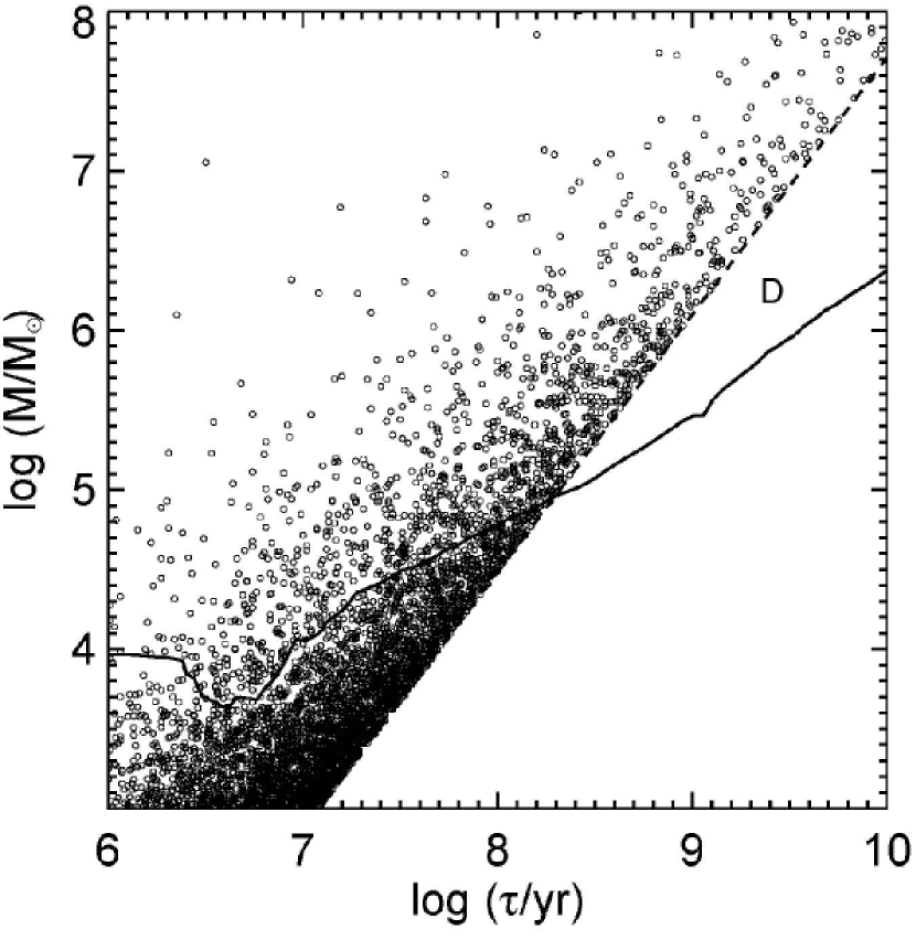
Figure 5: Mass-age plane for a simulated population of clusters based on Model 1. This has a power-law initial mass function, a constant formation rate, and sudden mass-dependent disruption with $\tau_{*}=5\times 10^{7}$ yr and $k=0.62$ in equation (7). The solid line is the approximate upper limit for stellar contamination ($L=3\times 10^{5}L_{\odot}$), while the dashed line indicates the age at which clusters are destroyed. The number of clusters in the simulated population above the solid line is approximately the same as in the real Antennae population. The region marked D here is empty, in contrast to the same region of Fig. 2.

We first consider Model 1, which assumes that clusters are disrupted suddenly at a mass-dependent age $\tau_{d}(M)=\tau_{*}(M/M_{*})^{k}$. It is instructive first to display the predictions of this model in the $M$–$\tau$ plane. Figure 5 shows a Monte Carlo realization of a cluster population generated by Model 1 with $\beta=-2$, $\tau_{*}=5\times 10^{7}$ yr, and $k=0.62$. It has been suggested that this value of $k$ may be ubiquitous among the cluster systems of different galaxies (Boutloukos & Lamers 2003). In this model, lower mass clusters are destroyed sooner than higher mass clusters, resulting in a sharp, diagonal line beyond which no clusters survive. The index $k$ regulates the slope of this line (proportional to $1/k$), while $\tau_{*}$ controls its intercept. Model 1 predicts an evacuated, triangular region to the right of the disruption line (marked D in Fig. 5). However, no such feature appears in Figure 2, the observed $M$–$\tau$ plane for the Antennae clusters. Thus, we can immediately rule out Model 1, at least for the mass-age domain studied here.

Despite this failure of Model 1, it is still instructive to compare the predicted and observed $\bar{g}(M)$ and $\bar{g}(\tau)$ distributions as a prelude to tests of the more realistic Models 2 and 3. Figures 6 and 7 show these comparisons for the same parameters adopted in Figure 5. Evidently, the shapes of the predicted and observed $\bar{g}(M)$ distributions match for sufficiently large $\tau_{*}$ (i.e. $\tau_{*}{\>\hbox to0.0pt{\raise 2.0pt\hbox{$>$}\hss}\lower 3.0pt\hbox{$\sim$}\>}5\times 10^{7}$ yr), ensuring that the predicted curvature occurs below the observed mass range. However, the amplitudes cannot be matched; the predicted amplitude is constant with age because, in the model, there is no evolution until clusters are suddenly disrupted, whereas the observed amplitude decreases substantially with age. The opposite problem arises with the $\bar{g}(\tau)$ distribution. In this case, the predicted and observed amplitudes agree (a direct consequence of the adopted initial mass function, $\psi_{0}(M)\propto M^{-2}$), but the shapes are quite different; the observations decline approximately like a power law in age, while the predictions remain flat for a while and then drop rapidly near the disruption time $\tau_{d}$ for clusters with the relevant mass ($M_{1}<M<M_{2}$). This behavior is generic: $\bar{g}(\tau)$ is predicted to have a sharp bend at $\tau_{d}$, but none is observed. Thus, we confirm our earlier conclusion that Model 1 does not describe the population of massive young clusters in the Antennae.

3.4 Comparison with Model 2: Gradual Mass-Dependent Disruption

Model 2 retains the power-law dependence of the disruption timescale on mass but smooths out the discontinuous evolution postulated by Model 1. As a result of this smoothness, one might guess that Model 2 would fare better against the observations than Model 1, but this turns out not to be true, as we now demonstrate. In Figures 8, 9, and 10, we compare the predicted $\bar{g}(M)$ from Model 2 for $k=0$, 0.6, and 1.0, respectively, with our Antennae observations. In the limit $k=0$, the disruption rate is independent of mass. In this case (Fig. 8), the predicted and observed $\bar{g}(M)$ match in shape for all values of $\tau_{*}$ but in amplitude only for $\tau_{*}\approx 1.4\times 10^{7}$ yr. However, with this value of $\tau_{*}$ (or any other), the predicted $\bar{g}(\tau)$ fails to reproduce the observed one, as shown in Figure 11. The reason for this is that, with the disruption law postulated by Model 2 (eqs. [8] and [9]), there is always a bend near $\tau_{d}$ in $M(\tau)$ (eq. [10]) and hence in $\bar{g}(\tau)$ (eqs. [B6] and [B7]), whereas the observations show no such feature. In the mass-dependent cases, $k=0.6$ (Fig. 9) and $k=1.0$ (Fig. 10), the predicted $\bar{g}(M)$ matches the observed one in shape for large enough $\tau_{*}$, so that the predicted curvature occurs below the observed mass range, but it never matches in amplitude for clusters both younger and older than $10^{7}$ yr. These are essentially the same problems that afflicted Model 1, with relatively minor differences resulting from the different disruption laws (one sudden, one gradual). We conclude, therefore, that Model 2 also fails to describe the Antennae clusters in the mass-age domain studied here.

This leads us to a more general consideration of mass-dependent disruption. We have shown that the observed mass function of star clusters in the Antennae has the same shape but different amplitude for different ages, while the observed age distribution has the same shape but different amplitude for different masses. These facts cannot be explained by mass-dependent disruption. In particular, if low-mass clusters were disrupted faster than high-mass clusters, the mass function would become flatter with increasing age; and conversely, if disruption had the opposite dependence on mass, the mass function would become steeper. Neither effect is observed in the mass function of the Antennae clusters. Furthermore, there are no discernible features in the observed mass and age distributions, as would be expected if the rate of disruption changed at a characteristic mass or age. We emphasize that these conclusions are not affected by the formation history of the clusters (i.e., whether they form at a constant or variable rate), provided only that the shape of their initial mass function is invariant. In this case, variations in the formation rate would affect only the amplitude of the mass function, but not its shape, at different ages. Thus, we conclude, quite generally, that disruption of the massive young clusters in the Antennae has little or no dependence on mass.

3.5 Comparison with Model 3: Gradual Mass-Independent Disruption

Model 3, with mass-independent disruption, was designed to remedy the problems encountered in fitting Models 1 and 2 to the Antennae data. As we noted in Section 2, the disruption of the population of clusters is gradual in this model, although the disruption of individual clusters may be gradual or sudden. This model also has fewer adjustable parameters ($C$, $\beta$, $\gamma$) than the other models ($C$, $\beta$, $k$, $\tau_{*}$). In Model 3, the averages over $g(M,\tau)$ are pure power laws: $\bar{g}(M)\propto M^{\beta}$ and $\bar{g}(\tau)\propto\tau^{\gamma}$. As Figures 12 and 13 show, the predicted and observed $\bar{g}(M)$ and $\bar{g}(\tau)$ agree nicely, both in shape and amplitude, for $\beta=-2.0$ and $\gamma=-1.0$. These results corroborate those from our earlier studies of the Antennae clusters (ZF99, FCW05, WCF07). Model 3 provides an excellent description of the population of massive young clusters in the Antennae. We note that the domain of validity of this result—the region of the $M$–$\tau$ plane above the stellar contamination limit—covers a relatively wide range of masses for very young clusters but becomes progressively narrower with increasing age, as shown in Figure 2 and approximated by equation (2). Thus, we regard Model 3 as a robust description of the observations for $\tau{\>\hbox to0.0pt{\raise 2.0pt\hbox{$<$}\hss}\lower 3.0pt\hbox{$\sim$}\>}10^{8}$ yr and more akin to an extrapolation for $\tau{\>\hbox to0.0pt{\raise 2.0pt\hbox{$>$}\hss}\lower 3.0pt\hbox{$\sim$}\>}10^{8}$ yr.

4 INTERPRETATION AND IMPLICATIONS

We showed in the previous section that the joint distribution of masses and ages of massive young clusters in the Antennae can be approximated by the simple formula $g(M,\tau)\propto M^{-2}\tau^{-1}$. This means that the shape of the mass function $\psi(M)\propto M^{-2}$ is independent of age and that the shape of the age distribution $\chi(\tau)\propto\tau^{-1}$ is independent of mass (at least over the observed domain of $M$ and $\tau$). We now seek to understand these results in terms of the physical processes that operated during the formation and early evolution of the clusters. We also consider the long-term future evolution of the young clusters and whether their mass function will eventually resemble that of old globular clusters. The picture presented here is an extension of the one proposed by Harris & Pudritz (1994) and Elmegreen & Efremov (1997) and developed in some of our earlier papers (ZF99; Fall & Zhang 2001; FCW05).

4.1 Formation of Star Clusters from Molecular Clouds

The mass functions of young star clusters must depend in some way on the mass functions of the molecular clouds in which they formed. Blitz et al. (2007) review CO observations of molecular clouds in several galaxies in the Local Group: the Milky Way, LMC, SMC, M31, M33, and IC10. The mass functions of the clouds can be represented by power laws, $dN/dM\propto M^{\beta}$, with $\beta\approx-1.7$ in most cases. The exceptions are M33, which has $\beta\approx-2.5$, and the SMC, which has too few clouds to estimate $\beta$. The range of masses covered by these observations varies substantially, from a $\mbox{few}\times 10^{5}~{}M_{\odot}{\>\hbox to0.0pt{\raise 2.0pt\hbox{$<$}\hss}\lower 3.0pt\hbox{$\sim$}\>}M{\>\hbox to0.0pt{\raise 2.0pt\hbox{$<$}\hss}\lower 3.0pt\hbox{$\sim$}\>}10^{6}~{}M_{\odot}$ for M33 to $10^{3}~{}M_{\odot}{\>\hbox to0.0pt{\raise 2.0pt\hbox{$<$}\hss}\lower 3.0pt\hbox{$\sim$}\>}M{\>\hbox to0.0pt{\raise 2.0pt\hbox{$<$}\hss}\lower 3.0pt\hbox{$\sim$}\>}\mbox{few}\times 10^{6}~{}M_{\odot}$ for the Milky Way. For complexes of molecular clouds in the Antennae, Wilson et al. (2003) find $\beta\approx-1.4$ (for $M{\>\hbox to0.0pt{\raise 2.0pt\hbox{$>$}\hss}\lower 3.0pt\hbox{$\sim$}\>}10^{7}~{}M_{\odot}$). While these estimates of $\beta$ are suggestive, it is worth noting that they pertain to clouds with relatively low column density thresholds (compared with the regions of most intense star formation) and, in the case of the Antennae, may also suffer from blending as a result of the larger distance and hence lower spatial resolution.

It is also interesting at this stage to recall some results for protoclusters in other galaxies. Studies of HII regions and OB associations in the Milky Way and many nearby galaxies show that their H$\alpha$ and Lyc luminosity functions have power-law form, $dN/dL\propto L^{\alpha}$, with exponents near $\alpha=-2$ (Kennicutt et al. 1989; McKee & Williams 1997). There appear to be small differences among the exponents for different galaxies and in some cases a high-luminosity turnover or cutoff. As we have noted before, luminosity and mass functions in general are not the same, due to the spread in ages and fading of the clusters. However, for HII regions and OB associations, the age spread is relatively narrow ($\tau\lesssim 10^{7}$ yr), the $M/L$ variations are modest, and luminosity functions become effective proxies for mass functions. Dowell et al. (2008) have derived the mass functions of young clusters ($\tau\lesssim 2\times 10^{7}$ yr) in several nearby galaxies based on broadband multi-color photometry (by a method generally similar to ours but using ground-based rather than $HST$ data). For $M\gtrsim{\rm few}\times 10^{4}M_{\odot}$, they find $dN/dM\propto M^{\beta}$, with $\beta=-1.9$ for their combined sample of irregular galaxies and $\beta=-1.8$ for their combined sample of spiral galaxies. We find $\beta\approx-1.8$ for the young clusters in the LMC (CFW09).

It is remarkable that all these mass functions are power laws with nearly the same exponent, $\beta\approx-2$. There may be small but real differences between the mass functions of molecular clouds and young star clusters in general and/or between the mass functions of either clouds or clusters in different galaxies, at the level $\Delta\beta\approx 0.2$–0.6. The significance of these differences is low, typically 1–3 $\sigma$, based on the statistical and likely systematic uncertainties in $\beta$. We also note that the different mass functions were determined by different researchers using different methods and that they pertain to different density thresholds and mass ranges. Thus it is possible that they are all basically the same, or more conservatively, that any differences between them are barely detectable. This means that the average efficiency of star formation in protoclusters—the ratio of the final stellar mass to the initial interstellar mass—is approximately independent of the mass of the protoclusters. If the efficiency varies at all, it decreases with increasing mass, since the mass functions of molecular clouds appear to be slightly flatter than the mass functions of young clusters. On average, low-mass protoclusters make stars just about as efficiently as high-mass protoclusters. This is a simple but important empirical result, which should help to guide theories of star and cluster formation. Indeed, it probably reflects a balance between star formation and stellar feedback within protoclusters (Elmegreen & Efremov 1997; Krumholz et al. 2006).

A complete understanding of the mass functions of young star clusters clearly requires an understanding of the mass functions of their progenitor molecular clouds. The ISM is often described as a turbulent medium in which the density and velocity fluctuations on each spatial scale mimic those on other scales in a self-similar hierarchy (see the reviews by Elmegreen & Scalo 2004 and McKee & Ostriker 2007). Given this picture, it is not surprising that the mass function of molecular clouds is a power law. The important question is what physical processes determine the exponent $\beta$. Fleck (1996) has derived $\beta=-2$ for relatively diffuse, non-self-gravitating clouds based on a simple analytical model of compressible turbulence in the ISM. Wada et al. (2000) find $\beta=-1.7$ in their 2D hydrodynamic simulations of ISM turbulence without stellar feedback and slightly steeper mass functions when feedback is included (see also Vázquez-Semadeni et al. 1997). Elmegreen (2002) finds $\beta\approx-2$ in his static models of a fractal ISM, and slightly steeper (shallower) mass functions for clouds with higher (lower) density thresholds. Despite these results, it is not yet entirely clear why the mass function of real molecular clouds has $\beta\approx-2$ rather than $\beta\approx-3$ or $\beta\approx-1$ (say). Explaining the physical origin of this exponent remains an important theoretical challenge.

4.2 Early Disruption: Processes and Timescales

Interstellar material is removed from protoclusters by feedback from massive stars (photoionization, radiation pressure, stellar winds, and supernovae). Observationally, the dividing line between protoclusters that contain interstellar material and those that do not is roughly $\tau\sim 10^{7}$ yr, based on the coincidence of molecular clouds and HII regions with the locations of clusters of different ages (Blitz et al. 2007). This timescale also makes sense from a physical point of view; it is a few multiples of the lifetimes of the most massive stars and about an order of magnitude longer than the dynamical or crossing times within the clusters. An important consequence of this early, rapid mass loss is that many of the protoclusters cannot remain gravitationally bound and therefore begin to dissolve almost as soon as they form (Hills 1980), a process often called “infant mortality.” In reality, the removal of ISM by stellar feedback will unbind some protoclusters completely and others only partially, leaving behind less-massive, but bound remnants. This process obviously affects the age distribution and hence the amplitude of the mass function of young clusters. But does it also affect the shape of the mass function?

It has been proposed that ISM removal disrupts a higher proportion of low-mass clusters than high-mass clusters, and that this introduces a bend or flattening in the mass function at $\sim 10^{5}M_{\odot}$ (Kroupa & Boily 2002; Baumgardt et al. 2008; Parmentier et al. 2008). We believe these claims are based on unrealistic models of protoclusters (see below). However, it is an easy matter to check observationally whether or not they are correct, by comparing the mass functions of Antennae clusters in the two age bins divided at $\tau=10^{7}$ yr (Figure 3). These show no hint of a bend; the power-law form of the mass function in the older bin appears identical to that in the younger bin, as we have already noted. If infant mortality imprints any feature in the mass function at all, it must be well below $10^{5}M_{\odot}$ and probably below $10^{4}M_{\odot}$ (to avoid any hint of curvature). We obtain even stronger constraints on mass-dependent disruption in our recent study of the clusters in the LMC (CFW09).

The shape of the mass function of young clusters depends on how effectively stellar feedback removes the ISM from protoclusters of different masses. This in turn depends on the fraction of the input energy that is radiated away from the protoclusters as a function of their mass. Most of the internal kinetic energy of molecular clouds is in the form of supersonic turbulence, which is dissipated in strong shocks on the dynamical timescales of the clouds (McKee & Ostriker 2007 and references therein). This important energy sink is not included in the models proposed by Kroupa & Boily (2002), Baumgardt et al. (2008), and Parmentier et al. (2008). Thus, it is likely that they have overestimated the energy available for disrupting protoclusters, possibly by large factors. In the limit of no radiative losses, the feedback is energy-driven, whereas in the opposite limit of maximum losses, it is momentum-driven. The second regime is likely to be more realistic than the first, and further analysis is needed to determine whether such feedback would imprint any features on the mass function of young clusters. Preliminary indications are that it would not (S. M. Fall et al. 2009, in preparation).

The preceding discussion of infant mortality presumes that the molecular clouds in which star clusters formed were gravitationally bound for at least some time before the onset of stellar feedback. This picture, however, is now debated (see the reviews by Elmegreen & Scalo 2004 and McKee & Ostriker 2007). It is possible instead that some of the sites of star and cluster formation are merely transient molecular concentrations created by convergent flows in the interstellar turbulence. The protoclusters produced at these sites might be unbound from the beginning, irrespective of any stellar feedback that occurs within them. This cannot be the whole story, of course, because at least a small fraction of clusters—those that survive for many of their own crossing times—must have formed as gravitationally bound objects. The revised picture in which some protoclusters are initially bound while others are unbound has not yet been studied in enough detail to make firm predictions about the shape of the resulting mass function of the surviving clusters. In a scale-free (fractal) ISM, however, there is no immediate reason to suspect that the fractions of bound and unbound clusters would change abruptly at a preferred mass scale or would even depend on mass at all.

The young clusters will continue to lose mass through stellar winds and other ejecta even after they have expelled all their nascent interstellar material. Stellar evolution alone depletes the masses of star clusters by $\sim$40% over a period of a ${\rm few}\times 10^{8}$ yr, although most of this mass is lost in the first ${\rm few}\times 10^{7}$ yr, the exact fraction and timescale depending on the shape of the stellar IMF. This process can unbind clusters in a tidal field if they are already weakly bound, with concentration parameters [$c\equiv\log(r_{t}/r_{c})$] in the range $c\lesssim 0.7$ (corresponding to dimensionless central potentials in the range $W_{0}{\>\hbox to0.0pt{\raise 2.0pt\hbox{$<$}\hss}\lower 3.0pt\hbox{$\sim$}\>}3$; Chernoff & Weinberg 1990; Fukushige & Heggie 1995; Takahashi & Portegies Zwart 2000). As a result of the prior removal of interstellar material, we expect many of the surviving clusters to be only weakly bound and thus vulnerable to disruption by subsequent stellar mass loss. If the concentration parameters of the clusters are uncorrelated with their masses (the simplest possibility), a large fraction of them could be disrupted in the period $10^{7}~{}\mbox{yr}\lesssim\tau\lesssim 10^{8}$ yr, without altering the power-law shape of the mass function, consistent with our observations of the Antennae and LMC clusters. In contrast, Vesperini & Zepf (2003) have argued that this process would produce a “bell-shaped” mass function. They base this claim on an assumed strong correlation between concentration and mass for young clusters, a hypothesis for which there is no physical explanation or observational evidence. The old globular clusters in the Milky Way do have such a correlation, but this is almost certainly a product of internal dynamical evolution over a Hubble time, including core collapse, tidal heating, and so forth. In any case, the similar shapes of the mass functions of clusters younger and older than $10^{7}$ yr in both the Antennae and the LMC tell heavily against this suggestion.

Another mechanism for disrupting star clusters is tidal disturbances by passing molecular clouds (Spitzer 1958). We follow the comprehensive treatment by Binney & Tremaine (2008, Sec 8.2) and distinguish two regimes: catastrophic, in which clusters are disrupted suddenly by a single strong encounter, and diffusive, in which clusters are disrupted gradually by a sequence of weak encounters. The disruption timescales in these regimes (up to proportionality) are

$$t_{\rm d}\propto\frac{\rho_{\rm h}^{1/2}}{M_{\rm p}n_{\rm p}}\,\,\,\,\,\,\,\,\,\,\,\,\,\,\,~{}~{}~{}~{}~{}~{}~{}~{}~{}~{}{\rm(catastrophic~{}regime)},$$ (16)

$$t_{\rm d}\propto\frac{\sigma_{\rm rel}r_{\rm hp}^{2}\rho_{\rm h}}{M_{\rm p}^{2}n_{\rm p}}\,\,\,\,\,\,\,\,\,\,\,\,\,\,\,~{}~{}~{}~{}~{}~{}~{}~{}~{}~{}~{}{\rm(diffusive~{}regime)}.$$ (17)

Here, $\rho_{\rm h}\equiv 3M/(8\pi r_{\rm h}^{3})$ is the mean density within the half-mass radius $r_{\rm h}$ of the clusters, $M_{\rm p}$, $r_{\rm hp}$, and $n_{\rm p}$ are the mass, half-mass radius, and mean number density of the molecular clouds (the perturbers), respectively, and $\sigma_{\rm rel}$ is the dispersion of the relative velocities between the clusters and clouds. Equations (16) and (17) display two important consequences of tidal disruption: (1) In both regimes, $t_{\rm d}$ depends on the masses $M$ of the clusters only through their mean internal densities $\rho_{\rm h}$; (2) In the catastrophic regime, $t_{\rm d}$ depends on the properties of the molecular clouds only through their mean smoothed-out density, $\bar{\rho}_{\rm p}\equiv M_{\rm p}n_{\rm p}$. For open clusters in the solar neighborhood, Binney & Tremaine (2008) estimate $t_{\rm d}\sim 3\times 10^{8}$ yr (in the catastrophic regime). This might provide a rough indication of what to expect in the Antennae galaxies, since $\rho_{\rm h}$ and $\bar{\rho}_{\rm p}$ might also be similar to their local values. If so, tidal disturbances would be effective in disrupting clusters older than $\sim 10^{8}$ yr in the Antennae. Despite the large uncertainty in the timescale for this process, we do not expect it to alter the shape of the mass function, since the mean internal densities of the clusters are fixed mainly by the galactic tidal field and should therefore be approximately the same for clusters of different masses.

We argued in the Introduction that the age distribution $\chi(\tau)$ primarily reflects the disruption history rather than the formation history of the clusters. The disruption history in turn is likely dominated by different physical processes in different intervals of age. Based on our previous discussion, the following sequence seems plausible: (1) disruption by removal of ISM, $\tau\lesssim 10^{7}$ yr; (2) disruption by stellar mass loss, $10^{7}{\rm yr}\lesssim\tau\lesssim 10^{8}{\rm yr}$; (3) disruption by tidal disturbances, $\tau\gtrsim 10^{8}$ yr. It also seems likely that the rate of disruption and hence the shape of the age distribution varies from one of these regimes to another, with some sort of features at the transitions between them. However, this combination of disruption processes involves too many unknowns to predict how prominent such features would be. As we have already noted, the uncertainties in the ages of the clusters preclude the measurement of fine structure in the age distribution, especially near the likely transition between disruption dominated by ISM removal and by stellar mass loss, at $\tau\sim 10^{7}$ yr. Moreover, the tail of $\chi(\tau)$ potentially dominated by tidal disturbances, at $\tau\gtrsim 10^{8}$ yr, is based on observations near the limit of our sample, where the accessible range of masses is relatively small. Plausible variations in the formation rate could also make the age distribution slightly flatter or slightly steeper. Thus, it is likely that our power-law model, $\chi(\tau)\propto\tau^{-1}$, is a simple approximation to a complex situation involving several different physical processes rather than an exact description of a single process. In any case, since the shape of the mass function is preserved by each of these processes, it will also be preserved by any combination of them.

4.3 Late Disruption of Clusters: Evaporation

As we already noted, a primary motivation for the present study has been to understand the formation and early evolution of star clusters in an environment similar to that during the early phases of the hierarchical assembly of galaxies, when the clusters that are now classified as old globular clusters were originally produced. Thus, we are led to speculate on the long-term future evolution of the young clusters in the Antennae, those that survive the first $\sim 10^{8}$ yr, over the next $\sim 10^{10}$ yr or so. A major issue here is that the mass functions of the young and old clusters are very different, and this immediately raises the question whether the former would evolve by long-term disruptive processes into the latter.

The upper panel of Figure 14 shows the mass functions of the young clusters in the Antennae and the LMC (both samples restricted to $\tau\lesssim 10^{8}$ yr). Here, we have plotted $dN/d\log{M}$ rather than $dN/dM$, as in our previous figures. The mass function for the Antennae clusters is taken from the present paper, while that for the LMC clusters is taken from our companion paper (CFW09), with a vertical shift to allow for the different sizes of the two populations. Both functions have the same power-law shape, although they cover different ranges of mass (higher in the Antennae, lower in the LMC). The upper smooth curves in both panels of Figure 14 are the same Schechter function, $\psi_{0}(M)\propto M^{\beta}\exp(-M/M_{c})$, with the parameters $\beta=-2$ and $M_{c}=2\times 10^{6}M_{\odot}$. We have appended the subscript 0 to $\psi$ to indicate that we will adopt this as the “initial” mass function in the calculation that follows. Evidently, we can represent the mass functions of young clusters over the observed range of masses equally well by a pure power law or a Schechter function with a sufficiently large cutoff $M_{c}$. In the present context, the Schechter function is preferable because it provides a better fit to the high-mass end of the mass function of old globular clusters, shown in the lower panel of Figure 14 (see also Burkert & Smith 2000; Jordán et al. 2007).

The most important long-term disruptive process operating on clusters is the gradual escape of stars driven by internal two-body relaxation (“evaporation”). This process depletes the mass of each cluster approximately linearly with time, $M(t)\approx M_{0}-\mu_{ev}t$, at a rate $\mu_{ev}$ that depends primarily on the mean internal volume or surface density of the cluster ($\mu_{ev}\propto\rho_{t}^{1/2}$ with $\rho_{t}\propto M/r_{t}^{3}$ for standard evaporation, $\mu_{ev}\propto\Sigma_{t}^{3/4}$ with $\Sigma_{t}\propto M/r_{t}^{2}$ for retarded evaporation; see Fig. 6 and eq. (12) of Baumgardt & Makino 2003 for the linearity of $M(t)$ and McLaughlin & Fall 2008 for the dependence of $\mu_{ev}$ on $\rho_{t}$ and $\Sigma_{t}$). The mass function of clusters with the same internal density at an age $\tau$ is then related to the initial mass function by the simple formula

$$\psi(M,\tau) \approx \psi_{0}(M+\mu_{ev}\tau)$$

$$\propto (M+\mu_{ev}\tau)^{\beta}\exp[-(M+\mu_{ev}\tau)/M_{c}]$$

(Fall & Zhang 2001; Jordán et al. 2007). For a population of clusters with different internal densities, and hence evaporation rates, the mass function is a superposition of terms like the one above, each with its own value of $\mu_{ev}$. Here, we approximate this superposition by a single term with a typical value of $\mu_{ev}$ for the whole population, which we have checked is sufficiently accurate for our present, illustrative purposes (see McLaughlin & Fall 2008 for a comprehensive discussion of these issues).

Two other long-term disruptive processes that are sometimes invoked are gravitational shocks (during passages through a galactic disk or near a galactic bulge) and dynamical friction. Gravitational shocks may be important for some massive clusters, but they are negligible compared with evaporation for low-mass clusters, in particular, those with masses near and below the turnover in the mass function i.e., $M\lesssim 10^{5}~{}M_{\odot}$ (Fall & Zhang 2001). Furthermore, gravitational shocks alone cannot change the shape of the mass function. Dynamical friction is only important in a massive galaxy, such as the eventual remnant of the merging Antennae, for a few very massive clusters located very near the galactic center and can safely be neglected for all the other clusters in a first approximation (Fall & Zhang 2001; Binney & Tremaine 2008). Tidal encounters with molecular clouds can also be neglected once the clusters are dispersed out of the disks of the merging galaxies and into the spheroid or halo of the remnant galaxy (at $\tau\sim 10^{9}$ yr or earlier).

The lower panel of Figure 14 shows the mass functions of the old globular clusters in the Milky Way and the Sombrero galaxy, again plotted as $dN/d\log{M}$. Both mass functions are derived from the corresponding luminosity functions, based on data from Harris (1996, as updated at http://www.mcmaster.ca/ $\tilde{}$harris/mwgc.dat) and Spitler et al. (2006), respectively, with an assumed mass-to-light ratio $M/L_{V}=1.5M_{\odot}/L_{\odot}$, a typical value obtained in dynamical studies (McLaughlin 2000). Again, the mass functions were shifted vertically to allow for the different sizes of the populations; and again both functions have similar shapes, although they cover somewhat different ranges of mass. With increasing mass, these functions first rise approximately linearly ($dN/d\log{M}\propto M$, corresponding to $dN/dM\approx{\rm const}$), reach a peak at $M_{p}\approx(1-2)\times 10^{5}~{}M_{\odot}$, and then decline steeply. The five solid curves in each panel of Figure 14 are the predictions of the simple evaporation model, equation (18) with $\mu_{ev}=2\times 10^{-5}M_{\odot}~{}{\rm yr}^{-1}$ and $\tau=0$, 1.5, 3, 6, and 12 Gyr. This value of $\mu_{ev}$ corresponds to an escape rate of 5%–10% per relaxation time, as indicated by various Fokker-Planck, Monte-Carlo, and $N$-body simulations of the evaporation of tidally limited clusters, when combined with the typical observed internal densities of the globular clusters in the Milky Way and Sombrero galaxies (Chandar et al. 2007; McLaughlin & Fall 2008). Thus, the horizontal position of the models in Figure 14 is fixed to within $\pm 0.2$ or less in $\log{M}$. The vertical position of the models is fixed by the high-mass end of the observed mass function, where evolution can be neglected.

Evidently, the model $\psi(M,\tau)$ at $\tau=12$ Gyr coincides remarkably well with the observed mass function of old globular clusters over the full range of masses, from $\sim 10^{4}M_{\odot}$ to above $\sim 10^{6}M_{\odot}$. This is a very simple and gratifying result: starting with a population of massive young clusters like those in the Antennae and the LMC, and then letting evaporation take its toll for about 12 Gyr, leads inevitably to a population of old globular clusters like those in the Milky Way and the Sombrero galaxy. No other ingredients or mechanisms are needed. This conclusion contrasts sharply with some recent suggestions that the turnover or bend at $M\sim 10^{5}~{}M_{\odot}$ in the evolved mass function of old globular clusters is simply a relic of a similar feature in the mass function of young clusters (see, for example, Parmentier et al. 2008). There are two problems with this explanation: (1) The postulated bend in the “initial” mass function conflicts directly with observations, as we have shown here for the Antennae clusters (and was shown earlier by ZF99) and in a companion paper for the LMC clusters (CFW09). (2) The claimed mechanisms for producing a bend in the mass functions of young clusters are either physically unrealistic (neglecting radiative dissipation of turbulence), or unjustified (assuming a strong correlation between mass and concentration). We note that the model with a power-law initial mass function (i.e., without a bend) is both simpler and fully consistent with all relevant observations of old globular clusters, including the dependence of their evolved mass function on their internal densities and galactocentric positions (Chandar et al. 2007; McLaughlin & Fall 2008).

5 SUMMARY AND CONCLUSIONS

In this paper, we have derived analytical formulae for the bivariate mass-age distribution $g(M,\tau)$ for three idealized models of the formation and disruption of star clusters. We have also derived formulae for the corresponding averages of $g(M,\tau)$ over finite intervals of $M$ and $\tau$, denoted by $\bar{g}(\tau)$ and $\bar{g}(M)$ respectively. In all three models considered here, clusters are assumed to form with a power-law initial mass function at a constant rate. In the first two models, proposed by Boutloukos & Lamers (2003), clusters are disrupted on a timescale that depends on their masses as $\tau_{d}(M)\propto M^{k}$ with $k>0$, either suddenly (Model 1) or gradually (Model 2). In the third model, clusters are disrupted (suddenly or gradually) at a fractional rate independent of their masses, as indicated by our earlier studies of the Antennae clusters (ZF99, FCW05, WCF07). Model 3 has the remarkably simple bivariate distribution $g(M,\tau)\propto M^{\beta}\tau^{\gamma}$. The corresponding luminosity, mass, and age distributions are all pure power laws: $\phi(L)\propto L^{\alpha}$, $\psi(M)\propto M^{\beta}$, $\chi(\tau)\propto\tau^{\gamma}$.

We have compared Models 1, 2, and 3 with the empirical distributions of luminosities, masses, and ages for a large sample of star clusters in the Antennae galaxies. These are based on our UBVIH$\alpha$ photometry of point-like sources in images taken with the WFPC2 on HST and comparisons with stellar population models to estimate $M$ and $\tau$ for each source (after correcting for interstellar reddening). To distinguish clusters of stars from individual stars, we have restricted our sample for analysis to objects brighter than $M_{V}=-9$, corresponding to $L>3\times 10^{5}L_{\odot}$. This limit defines the domain of validity of the models in the $L$-$\tau$ and $M$–$\tau$ planes, the regions above the solid curves in Figures 1 and 2 respectively, corresponding approximately to $\tau\lesssim 10^{7}(M/10^{4}M_{\odot})^{1.3}$ yr. Thus, all the results presented in this paper pertain to relatively massive and relatively young clusters (except in §4.3).

We find that Model 3, with mass-independent disruption, provides a good match to the observed mass-age distribution of the Antennae clusters. The best-fitting exponents in this model are $\beta\approx-2$ and $\gamma\approx-1$. Models 1 and 2, with mass-dependent disruption fare much worse. Even with complete freedom to adjust several parameters, these models never come close to matching the data. While our detailed comparisons are based on models in which the formation rates of clusters are constant, our main conclusion, that the disruption rates do not depend on mass, is valid even if the formation rates are variable. As a check on these results, we have also rederived the luminosity function of the Antennae clusters. After corrections for interstellar extinction, we find a good fit to a pure power law, $\phi(L)\propto L^{\alpha}$, with $\alpha\approx-2$. The fact that the mass and luminosity functions are nearly identical power laws ($\alpha\approx\beta$) is a consequence of—and additional support for—the weak or nonexistent correlations between masses and ages, i.e., the decomposition $g(M,\tau)\propto\psi(M)\chi(\tau)$. We have also investigated recent claims that there are bends or other features in the mass and luminosity functions of the Antennae clusters (Fritze-von Alvensleben 1999; Mengel et al. 2005; Anders et al. 2007). We show that these features are artifacts of the ways the samples are defined and do not reflect physical processes involved in the formation and disruption of the clusters.

In an effort to understand the physical basis for our simple—but doubtless approximate—model for $g(M,\tau)$, we first note that the resulting mass function, $\psi(M)\propto M^{-2}$, resembles that of molecular clouds in nearby galaxies. This indicates that the efficiency of star formation in the clouds is roughly independent of their masses. We also consider a variety of processes that could disrupt the protoclusters and clusters: removal of ISM by stellar feedback, continued stellar mass loss, tidal disturbances by passing molecular clouds, gravitational shocks during rapid passages near the galactic bulge and through the galactic disk, orbital decay into the galactic center caused by dynamical friction, and stellar escape driven by internal two-body relaxation. We suggest that the massive young clusters in the Antennae galaxies are disrupted in the following approximate sequence: (1) ISM removal, $\tau\lesssim 10^{7}$ yr, (2) stellar mass loss, $10^{7}{\rm yr}\lesssim\tau\lesssim 10^{8}{\rm yr}$, (3) tidal disturbances, $\tau\gtrsim 10^{8}$ yr. We have argued on theoretical grounds that these processes would operate at rates roughly independent of the masses of the clusters, consistent with our empirically-based decomposition $g(M,\tau)\propto\psi(M)\chi(\tau)$ (which, however, is only well established for $\tau\lesssim 10^{8}$ yr). In combination, these processes plausibly account for the observed decline of the age distribution, $\chi(\tau)\propto\tau^{-1}$. In the longer term, after 12 Gyr or so, the escape of stars driven by two-body relaxation will preferentially disrupt low-mass clusters and imprint a peak or turnover in the evolved mass function at $M_{p}\approx(1-2)\times 10^{5}M_{\odot}$, similar to that for old globular clusters in the Milky Way and other galaxies.

How general is this picture? In the Introduction, we mentioned some circumstantial evidence in favor of its wide applicability: the statistics of embedded clusters in the solar neighborhood (Lada & Lada 2003), the luminosities of the brightest clusters in different galaxies (Larsen 2002; Whitmore 2003; WCF07), the similarity of the mass spectra of molecular clouds in different galaxies (Blitz et al. 2007), and the fact that the early disruption of protoclusters and clusters ($\tau\lesssim 10^{8}$ yr) is driven mainly by internal processes that depend weakly, if at all, on the properties of their host galaxies (§4 here). Furthermore, from a detailed study of the mass-age distributions of clusters in the LMC and SMC, we find results nearly identical to those presented here for the clusters in the Antennae (CFW09). This is a strong test because the Antennae and the Magellanic Clouds represent very different environments for star and cluster formation: two large interacting galaxies on one hand, two small, relatively quiescent galaxies on the other hand. Nevertheless, further tests of this picture in other galaxies would be beneficial. If this picture turns out to be generally valid, it will mean that the main difference between populations of young clusters is simply in the normalization of $g(M,\tau)$ and hence in the overall formation rate. From this perspective, the objects traditionally designated open, populous, globular, or super clusters would belong to a continuum, with mass and age as the most fundamental variables, and would not require different formation and/or disruption processes to account for their observed properties.

The picture presented here has the virtues of simplicity and possible universality. It captures the salient properties of the observed mass-age distribution, at least for the populations of clusters we have studied so far. Nevertheless, we do not expect our model $g(M,\tau)$ to be strictly universal. It may break down outside its domain of validity in most galaxies or inside this domain in some extreme environments, such as those dominated by population III stars. There may also be minor deviations from the model in some normal galaxies, even within the domain of validity, caused for example by variations in the formation rates and/or differences in the disruption rates by passing molecular clouds. However, these are only likely to affect $g(M,\tau)$ at intermediate ages ($10^{8}{\rm yr}\lesssim\tau\lesssim 10^{9}{\rm yr}$), which will be difficult to detect observationally. We see an analogy between, on one hand, the potentially universal stellar IMF, represented by a simple, approximate formula (first by Salpeter (1955) and then revised in subsequent studies based on more modern data) and, on the other hand, the potentially universal mass-age distribution $g(M,\tau)$ for star clusters, represented here by a simple, approximate formula. Both the stellar IMF and the cluster $g(M,\tau)$ are thought to be the outcome of several complex physical processes, in ways not yet fully understood, and neither is expected to hold exactly in all situations. Even so, these functions provide compact and useful summaries of the observations and are thus natural focal points for future studies of the formation and early evolution of stars and clusters.

Appendix A COMPARISON WITH OTHER WORKS

The mass and luminosity functions of star clusters in the Antennae galaxies derived in several other studies differ from the simple power laws presented here. However, as we demonstrate in this appendix, the claimed peaks, bends, and other deviations from power laws all result from incompleteness in the samples of clusters rather than from any physical processes involved in their formation or disruption. Before we discuss any specific claims for features in the mass and luminosity functions, however, it is worth considering the credibility of such claims in general. Features that appear near the luminosity limit or detection threshold should be considered with skepticism, as they are almost always due to incompleteness. Another common problem is selection criteria that fail to account for the fading of the clusters with age, or that are linked in some way to measurement errors. Finally, we note that it is inherently much more likely that selection effects or measurement errors would convert a simple underlying function like a power law into a more complicated one with extra features than the other way around.

These concerns are well founded in practice. Based on observations taken with the WF/PC1 on $HST$ (before the spherical aberration was corrected), Fritze-von Alvensleben (1999) claimed that the mass function of the young clusters in the Antennae galaxies had a lognormal form, with a peak at $M\sim 10^{5}M_{\odot}$, like that of old globular clusters. However, the purported peak was near the detection limit, and much deeper observations taken with the WFPC2 (after the correction of spherical aberration), showed that it was simply an artifact of incompleteness, and that the mass function was in fact well represented by a power law, $\psi(M)\propto M^{-2}$, over the full range of masses, $10^{4}M_{\odot}\lesssim M\lesssim 10^{6}M_{\odot}$ (ZF99 and §3.2 here).

Mengel et al. (2005) have presented a mass function for the Antennae clusters that exhibits a gradual bend at $M\sim 10^{5}~{}M_{\odot}$. Their result, derived from ground-based $K$-band observations, is reproduced here as the open triangles in the top panel of Figure 15. This is based on a sample that is limited at a constant luminosity with no restriction on age, instead of being limited at a variable luminosity, corresponding to a constant mass, and restricted to relatively narrow intervals of age, as in our procedure. Because the clusters fade with age, the Mengel et al. sample does not include the same range of masses at all ages; older, low-mass clusters will be missed as they fade below the luminosity limit. We illustrate this in the bottom panel of Figure 15, which shows a mass function constructed from our own sample but with a selection procedure like that of Mengel et al. Here, we have included clusters of all ages brighter than $K_{\rm lim}=19$ (open circles), where we have estimated the $K$-band magnitude of each cluster from the observed $V$-band magnitude and the $V-K$ color predicted by the stellar population models of Bruzual & Charlot (2003) for the age derived from our UBVIH$\alpha$ observations. Evidently, this selection procedure introduces a bend in the output mass functions similar to the one found by Mengel et al., even though the input mass function is a power law (see §3.2 and Fig. 3). We have also performed experiments with luminosities limited in the $V$ and other bands and with gradual and sharp cutoffs, and we always recover a similar, artificial bend in the mass function. Mengel et al. (2005) themselves appear to be aware of this problem and urge caution in interpreting the bend in their mass function as a real feature.

Anders et al. (2007) have derived a luminosity function of Antennae clusters with a peak near $M_{V}\approx-8.5$, based on the same WFPC2 observations used here but a very different selection procedure. In particular, they include only clusters with photometric errors $\leq 0.2$ mag in UBVI, thereby excluding many real clusters. Since most of the missing clusters are faint, the luminosity function derived in this way will fall below the true one at low luminosities, potentially introducing an artificial peak. To test for this, we have repeated the steps in the Anders et al. selection procedure, but using our own sample of clusters, for which the input luminosity function is known to be a power law (see §3.2 and Fig. 4). In this case, the output luminosity function resembles the one presented by Anders et al., with strong deviations from a power law, resulting primarily from the elimination of clusters with large uncertainties in the $U$-band photometry. Thus, we conclude that the purported peak is an artifact of this selection bias. A forthcoming study of the Antennae clusters based on deeper, higher-resolution observations taken with the ACS on HST confirms and extends the results presented in this paper, finding a luminosity function that is well represented by a pure power law with $\alpha\approx-2$ down to at least $M_{V}\approx-7$, with no evidence for a break or flattening near $M_{V}\approx-8.5$ (Whitmore et al. 2009).

Appendix B FORMULAE FOR $\bar{g}(M)$ and $\bar{g}(\tau)$

Here, we present formulae for $\bar{g}(M)$ and $\bar{g}(\tau)$, the averages of $g(M,\tau)$ over age ($\tau_{1}\leq\tau\leq\tau_{2}$) and mass ($M_{1}\leq M\leq M_{2}$), respectively, for the three disruption models discussed in Section 2. The equations that follow were derived from equations (6) and (12)–(15). The function $M_{d}(\tau)$ in equations (B3) and (B4) is the inverse of the function $\tau_{d}(M)$ in equations (B1) and (B2). The formulae for $\bar{g}(M)$ and $\bar{g}(\tau)$ are valid for the stated values of the exponents $k$ and $\gamma$ in the disruption models. They are valid for all values of the exponent of the initial mass function except $\beta=-1$, which is far enough from the observed value $\beta\approx-2$ to be irrelevant in the present context.

Model 1: Sudden Mass-Dependent Disruption.

$$\bar{g}(M)=C(M/M_{*})^{\beta}\left\{\begin{array}[]{ll}0&\mbox{for $\tau_{d}(M)<\tau_{1}$}\\ R(M)&\mbox{for $\tau_{1}\leq\tau_{d}(M)\leq\tau_{2}$}\\ 1&\mbox{for $\tau_{2}<\tau_{d}(M)$}\end{array}\right.$$ (B1)

$$R(M)=\frac{\tau_{d}(M)-\tau_{1}}{\tau_{2}-\tau_{1}}$$ (B2)

$$\bar{g}(\tau)=C_{1}\left\{\begin{array}[]{ll}1&\mbox{for $M_{d}(\tau)<M_{1}$}\\ S(\tau)&\mbox{for $M_{1}\leq M_{d}(\tau)\leq M_{2}$}\\ 0&\mbox{for $M_{2}<M_{d}(\tau)$}\end{array}\right.$$ (B3)

$$S(\tau)=\frac{M_{2}^{\beta+1}-M_{d}(\tau)^{\beta+1}}{M_{2}^{\beta+1}-M_{1}^{\beta+1}}$$ (B4)

$$C_{1}=\left(\frac{C}{\beta+1}\right)\left(\frac{M_{*}}{M_{2}-M_{1}}\right)\left[\left(\frac{M_{2}}{M_{*}}\right)^{\beta+1}-\left(\frac{M_{1}}{M_{*}}\right)^{\beta+1}\right]$$ (B5)

Model 2: Gradual Mass-Dependent Disruption.

$$\bar{g}(M)=C_{2}(M/M_{*})^{\beta+k}\left[T(M,\tau_{2})-T(M,\tau_{1})\right]\hskip 28.45274pt{\rm for}\,\,\,\,\,k\not=0$$ (B6)

$$T(M,\tau)=\left[1+k(M/M_{*})^{-k}(\tau/\tau_{*})\right]^{(\beta+1)/k}$$ (B7)

$$C_{2}=\left(\frac{C}{\beta+1}\right)\left(\frac{\tau_{*}}{\tau_{2}-\tau_{1}}\right)$$ (B8)

$$\bar{g}(M)=C_{3}(M/M_{*})^{\beta}\hskip 28.45274pt{\rm for}\,\,\,\,\,k=0$$ (B9)

$$C_{3}=\left(\frac{C}{\beta+1}\right)\left(\frac{\tau_{*}}{\tau_{2}-\tau_{1}}\right)\left\{\exp\left[(\beta+1)\left(\frac{\tau_{2}}{\tau_{*}}\right)\right]-\exp\left[(\beta+1)\left(\frac{\tau_{1}}{\tau_{*}}\right)\right]\right\}$$ (B10)

$$\bar{g}(\tau)=C_{1}\exp\left[(\beta+1)(\tau/\tau_{*})\right]\hskip 28.45274pt{\rm for}\,\,\,\,\,k=0$$ (B11)

Model 3: Gradual Mass-Independent Disruption.

$$\bar{g}(M)=C_{4}(M/M_{*})^{\beta}\hskip 28.45274pt{\rm for}\,\,\,\,\,\gamma\not=-1$$ (B12)

$$C_{4}=\left(\frac{C}{\gamma+1}\right)\left(\frac{\tau_{*}}{\tau_{2}-\tau_{1}}\right)\left[\left(\frac{\tau_{2}}{\tau_{*}}\right)^{\gamma+1}-\left(\frac{\tau_{1}}{\tau_{*}}\right)^{\gamma+1}\right]$$ (B13)

$$\bar{g}(M)=C_{5}(M/M_{*})^{\beta}\hskip 28.45274pt{\rm for}\,\,\,\,\,\gamma=-1$$ (B14)

$$C_{5}=C\left(\frac{\tau_{*}}{\tau_{2}-\tau_{1}}\right)\ln\left(\frac{\tau_{2}}{\tau_{1}}\right)$$ (B15)

$$\bar{g}(\tau)=C_{1}(\tau/\tau_{*})^{\gamma}\hskip 28.45274pt{\rm for}\,\,{\rm all}\,\,\gamma$$ (B16)

Figure 3: Mass function of Antennae clusters in the indicated intervals of age. The lines are power laws, $dN/dM\propto M^{\beta}$, with best-fit exponents $\beta=-2.14\pm 0.03$ (dashed) and $\beta=-2.03\pm 0.07$ (solid) for the younger and older clusters, respectively.

Figure 4: Luminosity function of Antennae clusters in the $V$ band, with and without corrections for extinction (as indicated). The lines are power laws, $dN/dL\propto L^{\alpha}$, with best-fit exponents $\alpha=-2.09\pm 0.05$ (dashed) and $\alpha=-2.37\pm 0.06$ (solid) for the corrected and uncorrected luminosities, respectively.

Figure 6: Mass distribution averaged over the indicated intervals of age for the Antennae clusters (data points) and for Model 1 (lines). In this model, clusters have a power-law initial mass function, a constant formation rate, and sudden mass-dependent disruption. The dashed and solid lines were computed for the younger and older clusters, respectively, from equations (7), (B1), and (B2) with $\tau_{*}=5\times 10^{7}$ yr and $k=0.62$.

Figure 7: Age distribution averaged over the indicated intervals of mass for the Antennae clusters (data points) and for Model 1 (lines). In this model, clusters have a power-law initial mass function, a constant formation rate, and sudden mass-dependent disruption. The dashed and solid lines were computed for less massive and more massive clusters, respectively, from equations (7) and (B3)–(B5) with $\tau_{*}=5\times 10^{7}$ yr and $k=0.62$.

Figure 8: Mass distribution averaged over the indicated intervals of age for the Antennae clusters (data points) and for Model 2 with $k=0$ (lines). In this model, clusters have a power-law initial mass function, a constant formation rate, and gradual mass-dependent disruption. The solid lines were computed for the older clusters only from equations (B9) and (B10) with the indicated values of $\tau_{*}$. The dashed line, with $\tau_{*}=1.4\times 10^{7}$ yr, provides a good fit to the observed distribution for the older clusters.

Figure 9: Mass distribution averaged over the indicated intervals of age for the Antennae clusters (data points) and for Model 2 with $k=0.6$ (lines). In this model, clusters have a power-law initial mass function, a constant formation rate, and gradual mass-dependent disruption. The solid lines were computed for the older clusters only from equations (B6)–(B8) with the indicated values of $\tau_{*}$.

Figure 10: Mass distribution averaged over the indicated intervals of age for the Antennae clusters (data points) and for Model 2 with $k=1.0$ (lines). In this model, clusters have a power-law initial mass function, a constant formation rate, and gradual mass-dependent disruption. The solid lines were computed for the older clusters only from equations (B6)–(B8) with the indicated values of $\tau_{*}$.

Figure 11: Age distribution averaged over the indicated interval of mass for the Antennae clusters (data points) and for Model 2 with $k=0$ (lines). In this model, clusters have a power-law initial mass function, a constant formation rate, and gradual mass-dependent disruption. The solid lines were computed from equations (B5) and (B11) with the indicated values of $\tau_{*}$. The dashed line here corresponds to the dashed line in Fig. 8 (both with $\tau_{*}=1.4\times 10^{7}$ yr).

Figure 12: Mass distribution averaged over the indicated intervals of age for the Antennae clusters (data points) and for Model 3 with $\gamma=-1.0$ (lines). In this model, clusters have a power-law initial mass function, a constant formation rate, and gradual mass-independent disruption. The dashed and solid lines were computed for the younger and older clusters, respectively, from equations (B14) and (B15).

Figure 13: Age distribution averaged over the indicated intervals of mass for the Antennae clusters (data points) and for Model 3 with $\gamma=-1.0$ (lines). In this model, clusters have a power-law initial mass function, a constant formation rate, and gradual mass-independent disruption. The dashed and solid lines were computed for the less massive and more massive clusters, respectively, from equations (B5) and (B16).

Figure 14: Mass functions of young clusters in the Antennae and LMC (upper panel) and old globular clusters in the Milky Way and Sombrero (lower panel), as described in the text. The smooth curves in both panels are from the simple evaporation model, eqn. (18) with $\mu_{ev}=2\times 10^{-5}M_{\odot}{\rm yr}^{-1}$, at ages $\tau=0$, 1.5, 3, 6, and 12 Gyr. Note the excellent fit of the model to the data at both $\tau=0$ (upper panel) and $\tau=12$ Gyr (lower panel).

Figure 15: Upper Panel: Mass function of Antennae clusters from this work (filled circles) and from Mengel et al. (2005) (open triangles). The former is based on an age-restricted subsample ($\tau=$ 1–10 Myr); the latter is based on a subsample limited in $K_{s}$-band luminosity but with no restriction on age. The vertical dashed line is the stated 50% completeness limit for the Mengel et al. sample ($K_{s}\approx 18.4$). Lower Panel: Mass function of Antennae clusters from this work (filled circles) and for a subsample with a luminosity limit similar to that of Mengel et al., based on $K_{s}$ magnitudes predicted from stellar population models and the observed $V$ magnitudes (open circles).

References

- (1) Anders, P., Bissantz, N., Boysen, L., de Grijs, R., & Fritze-von Alvensleben, U. 2007, MNRAS, 377, 91
- (2) Baumgardt, H., Kroupa, P., & Parmentier, G. 2008, MNRAS, 384, 1231
- (3) Baumgardt, H., & Makino, J. 2003, MNRAS, 340, 227
- (4) Binney, J., & Tremaine, S. 2008 Galactic Dynamics, 2nd Ed (Princeton: Princeton Univ. Press)
- (5) Blitz, L., Fukui, Y., Kawamura, A., Leroy, A., Mizuno, N., & Rosolowsky, E. 2007, in Protostars and Planets V, ed. B. Reipurth, D. Jewitt, & K. Keil (Tucson: Univ. Arizona Press), 81
- (6) Boutloukos, S. G., & Lamers, H. J. G. L. M. 2003, MNRAS, 338, 717
- (7) Bruzual, G., & Charlot, S. 2003, MNRAS, 344, 1000
- (8) Burkert, A., & Smith, G. H. 2000, ApJ, 542, L95
- (9) Calzetti, D., Kinney, A. L., & Storchi-Bergmann, T. 1994, ApJ, 429, 572
- (10) Chabrier, G. 2003, PASP, 115, 763
- (11) Chandar, R., Fall, S. M., & McLaughlin, D. E. 2007, ApJ, 668, L119
- (12) Chandar, R., Fall, S. M., & Whitmore, B. C. 2009, ApJ, submitted (CFW09)
- (13) Chernoff, D. F., & Weinberg, M. D. 1990, ApJ, 351, 121
- (14) Dowell, J. D., Buckalew, B. A., & Tan, J. C. 2008, AJ, 135, 823
- (15) Elmegreen, B. G. 2002, ApJ, 564, 773
- (16) Elmegreen, B. G., & Efremov, Y. N. 1997, ApJ, 480, 235
- (17) Elmegreen, B. G., & Scalo, J. 2004, ARA&A, 42, 211
- (18) Fall, S. M. 2006, ApJ, 652, 1129
- (19) Fall, S. M., Chandar, R., & Whitmore, B. C. 2005, ApJ, 631, L133 (FCW05)
- (20) Fall, S. M., & Zhang, Q. 2001, ApJ, 561, 751
- (21) Fitzpatrick, E. L. 1999, PASP, 111, 63
- (22) Fleck, R. C. 1996, ApJ, 458, 739
- (23) Fritze-von Alvensleben, U. 1999, A&A, 342, L25
- (24) Fukushige, T., & Heggie, D. C. 1995, MNRAS, 276, 206
- (25) Harris, W. E. 1996, AJ, 112, 1487
- (26) Harris, W. E., & Pudritz, R. E., 1994, ApJ, 429, 177
- (27) Hills, J. G. 1980, ApJ, 225, 986
- (28) Jordán, A., et al. 2007, ApJS, 171, 101
- (29) Kennicutt, R. C., Edgar, B. K., & Hodge, P. W. 1989, ApJ, 337, 761
- (30) Kroupa, P. 2001, MNRAS, 322, 231
- (31) Kroupa, P., & Boily, C. M. 2002, MNRAS, 336, 1188
- (32) Krumholz, M. R., Matzner, C. D., & McKee, C. F. 2006, ApJ, 653, 361
- (33) Lada, C. J., & Lada, E. A. 2003, ARA&A, 41, 57
- (34) Larsen, S. S. 2002, AJ, 124, 1393
- (35) Leitherer, C. et al. 1999, ApJS, 123, 3
- (36) Matzner, C. D., & McKee, C. F. 2000, ApJ, 545, 364
- (37) McKee, C. F., & Ostriker, E. C. 2007, ARA&A, 42, 211
- (38) McKee, C. F., & Williams, J. P. 1997, ApJ, 476, 144
- (39) McLaughlin, D. E. 2000, ApJ, 539, 618
- (40) McLaughlin, D. E., & Fall, S. M. 2008, ApJ, 679, 1272
- (41) Mengel, S., Lehnert, M. D., Thatte, N., & Genzel, R. 2005, A&A, 443, 41
- (42) Mihos, J. C., Bothun, G. D., & Richstone, D. O. 1993, ApJ, 418, 82
- (43) Parmentier, G., Goodwin, S. P., Kroupa, P., & Baumgardt, H. 2008, ApJ, 678, 347
- (44) Salpeter, E. 1955, ApJ, 121, 161
- (45) Spitler, L. R., Larsen, S. S., Strader, J., Brodie, J. P., Forbes, D. A., & Beasley, M. A. 2006, AJ, 132, 1593
- (46) Spitzer, L. 1958, ApJ, 127, 17
- (47) Spitzer, L. 1987, Dynamical Evolution of Globular Clusters (Princeton: Princeton Univ. Press)
- (48) Takahashi, K., & Portegies Zwart, S. F. 2000, ApJ, 535, 759
- (49) Vázquez-Semadeni, E., Ballesteros-Paredes, J., & Rodríguez, L. F. 1997, ApJ, 474, 292
- (50) Vesperini, E., & Zepf, S. E. 2003, ApJ, 587, L97
- (51) Vesperini, E., Zepf, S. E., Kundu, A., & Ashman, K. M. 2003, ApJ, 593, 760
- (52) Wada, K., Spaans, M., & Kim, S. 2000, ApJ, 540, 797
- (53) Whitmore, B. C. 2003, in A Decade of Hubble Space Telescope Science, ed. M. Livio, K. Noll, & M. Stiavelli (Cambridge: Cambridge Univ. Press), 153
- (54) Whitmore, B. C. 2004, in ASP Conf. Ser. 322, The Formation and Evolution of Massive Young Star Clusters, ed. H. J. G. L. M. Lamers, L. J. Smith, & A. Nota (San Francisco: ASP), 411
- (55) Whitmore, B. C., Chandar, R., & Fall, S. M. 2007, AJ, 133, 1067 (WCF07)
- (56) Whitmore, B. C., & Zhang, Q. 2002, AJ, 124, 1418
- (57) Whitmore, B. C., Zhang, Q., Leitherer, C., Fall, S. M., Schweizer, F., & Miller, B. W. 1999, AJ, 118, 1551
- (58) Whitmore, B. C., et al. 2009, AJ, submitted
- (59) Wilson, C. D., Scoville, N., Madden, S. C., & Charmandaris, V. 2003, ApJ, 599, 1049
- (60) Zhang, Q., & Fall, S. M. 1999, ApJ, 527, L81 (ZF99)