Wilson loops at finite N in 2D

Abstract:

Some exact expressions for non-selfintersecting Wilson loops in Yang Mills theory on the infinite plane are reviewed.

1 Introduction

Wilson loops need to be renormalized in 3D and 4D $SU(N)$ pure gauge theory. One way to do this, which is well defined outside perturbation theory too, is smearing [1, 2]. Wilson loop operators regularized by smearing satisfy all the constraints coming from the supposition that they are statistically distributed unitary matrices of unit determinant. In particular, one can define an eigenvalue density which will have support restricted to the unit circle for all loop sizes. Smeared Wilson loops in 3D and 4D $SU(N)$ gauge theory undergo an infinite-$N$ phase transition in their eigenvalue density at a specific loop size. At this size, a gap in the spectrum at -1 just closes. The transition is in the same universality class as in 2D, where it was discovered by Durhuus and Olesen in 1981 [3].

In 2D no smearing is needed because there are no perimeter divergences and the problem is exactly solvable. Consequently, also in 3D or 4D the eigenvalues close to -1 can be described by the equivalent 2D functions if $\infty>N\gg 1$ and if the loop size is close to critical.

I shall present some useful exact results in 2D for arbitrary finite $N$. These results provide a parametrization of the behavior of extremal Wilson loop eigenvalues in the crossover scale range separating small from large loops [4].

The hope is to use this to connect the two extreme regimes in 4D by a matched asymptotic expansion valid for $N\gg 1$: Suppose we accept that for $N\gg 1$ there exists a theory of open strings which would be free at $N=\infty$ and which can be used to write expressions for gauge theory observables like Wilson loops. The free string theory is not known, but for large distances it can be approximated by an effective string theory, starting form the Nambu action, and augmented by an infinite set of corrections ranked by powers of an inverse scale. The problem now becomes how to connect this effective theory at large distances to the theory at short distances which admits the standard perturbative expansion. More precisely, we wish to calculate the parameters of the effective string theory from standard field theory. Our main point is to establish that smeared Wilson loops are useful observables in that the transition from short scales to long scales becomes a phase transition at infinite $N$ with universal properties identical to the same type of transition in the exactly solvable 2D case. The universal regime ought to be matched onto expressions obtained from perturbation theory at short distances and onto expressions obtained from effective string theory at long distances. Knowledge of the universal functions describing the Wilson loop in the vicinity of the transition scale is the means by which unknown parameters in the string description could be expressed in terms of parameters of perturbation theory. The first challenge would be to calculate the string tension in units of $\Lambda_{SU(N)}$.

2 Probability density for Wilson loops in 2D

2.1 Averaging class functions

Wilson loops regularized by smearing can be thought of as expressed in terms of a fluctuating unitary matrix. More conventional regularizations will not admit such a picture because some inequalities obeyed by the trace of a unitary matrix will get violated. In two dimensions, there is no need to regularize the Wilson loops and smearing is not needed.

In 2D the probability density for a Wilson loop matrix $W$ is

$${\cal P}_{N}(W,t)=\sum_{r}d_{r}\chi_{r}(W)e^{-\frac{t}{2N}C_{2}(r)}$$ (1)

with $t=\lambda{\cal A}$ and $\lambda=g^{2}N$ the ’t Hooft coupling. $\cal A$ is the area enclosed by the loop. The loop is assumed to be smooth and non-self-intersecting. $d_{r}$, $C_{2}(r)$ and $\chi_{r}(W)$ are the dimension, quadratic Casimir and character for the irreducible representation $r$ of $SU(N)$, respectively. Unlike in higher dimensions, there is no dependence on the shape of the loop, only on its area.

Averages over $W$ at fixed $t$ are given by

$$\langle{\cal O}(W)\rangle=\int dW{\cal P}_{N}(W,t){\cal O}(W)$$ (2)

with Haar measure $dW$.

3 Eigenvalue behavior as a function of scale

3.1 Three observables – definitions

3.1.1 asym

The simplest observable is the generating function for all totally antisymmetric irreducible representations, described by single-column Young patterns:

$$\langle\det(z-W)\rangle,~{}~{}\tau\equiv t(1+1/N)\,.$$ (3)

3.1.2 sym

The second observable is the generating function for all totally symmetric irreducible representations, described by single-row Young patterns. This is the simplest observable that generates a smoothed out eigenvalue density for any $N$:

$$\langle\det(z-W)^{-1}\rangle,~{}~{}T\equiv t(1-1/N)\,.$$ (4)

3.1.3 true

The third observable is the generating function for all irreducible representations given by Young patterns of the following “hook” shape:

(5)

The quadratic Casimir for the above hook pattern is $C_{2}(p,q)$ and the dimension of the associated irreducible representation is $d(p,q)$, where $p,q\geq 0$. The observable is

$$\langle\det[(1+uW)/(1-vW)]\rangle\,.$$ (6)

From this observable one can extract the single-eigenvalue density of $W$ for any $N$.

3.2 Three observables – leading order in $1/N$

To leading order in large $N$ one has

$$\langle\det(z-W)^{-1}\rangle\approx\frac{1}{\langle\det(z-W)\rangle}\,,\quad\langle\det[(1+uW)/(1-vW)]\rangle\approx\frac{\langle\det(1+uW)\rangle}{\langle\det(1-vW)\rangle}\,.$$ (7)

3.3 Three observables – exact expressions

In each case, using character orthogonality, averaging produces a sum over all contributing characters of $W$.

3.3.1 asym

The density

$$\rho_{N}^{\tt asym}(\theta,\tau)=\frac{2\pi}{N}\sum_{j=0}^{N-1}\delta_{2\pi}(\theta-\theta_{j}(\tau))$$ (8)

is described by a sum of $N$ $\delta$-functions because $\langle\det(z-W)\rangle$ is a polynomial of rank $N$. This density is obtained from Eq. (3) as follows:

$$\Phi^{(N)}(z,\tau)=\frac{i}{N}\frac{\partial\log\langle\det(z-W)\rangle}{\partial\log z}+\frac{i}{2}\,,$$ (9)

$$\phi_{\pm}^{(N)}(\theta,\tau)=\lim_{\epsilon\searrow 0}\Phi^{(N)}(e^{-i(\theta\pm i\epsilon)},\tau)\,,$$ (10)

$$\rho_{N}^{\tt asym}(\theta,\tau)=-i\left[\phi_{+}^{(N)}(\theta,\tau)-\phi_{-}^{(N)}(\theta,\tau)\right].$$ (11)

The evolution of the angles is exactly described by a Calogero system:

$$\dot{\theta}_{j}=\frac{1}{2N}\sum_{k\neq j}\cot\frac{\theta_{j}-\theta_{k}}{2}\,,\quad\theta_{j}(0)=0\,.$$ (12)

Eigenvalues shoot out from the origin at $\tau=0$ and go round the unit circle until they relax exponentially into the locations of the $N$ roots of unity at $\tau=\infty$ [4].

3.3.2 asym: Burgers’ equation

Setting $\Phi_{N}(y,\tau)=-i\Phi^{(N)}(-e^{y},\tau)$ leads one to Burgers’ equation [5]:

$$\frac{\partial\Phi_{N}}{\partial\tau}+\Phi_{N}\frac{\partial\Phi_{N}}{\partial y}=\frac{1}{2N}\frac{\partial^{2}\Phi_{N}}{\partial y^{2}}\,,\quad\Phi_{N}(y,0)=-\frac{1}{2}\tanh\frac{y}{2}\,.$$ (13)

At $N=\infty$ a shock wave forms at $y=0$ and $\tau=4$; this is a well known property of Burgers’ equation [6]. The shock wave reflects the Durhuus and Olesen $N=\infty$ phase transition. They obtained their result from the inviscid limit of Burgers’ equation. The new result is that this particular observable satisfies the full equation of Burgers at finite $N$. The viscosity is equal to $\frac{1}{2N}$. Figure 1 shows how a shock develops as a result of a propagation velocity that depends linearly on the amplitude.

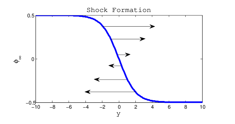
Figure 1: The making of a shock.

3.3.3 sym

The density associated with all the symmetric representations is given by

$$\rho_{N}^{\tt sym}(\theta,T)=1+\frac{1}{N}\left[p(\theta,T)+p^{\ast}(\theta,T)\right],$$ (14)

where

$$p(\theta,T)=\frac{\sum_{k=1}^{\infty}k{N+k-1\choose N-1}e^{ik\theta}e^{-T\frac{k(k+N)}{2N}}}{1+\sum_{k=1}^{\infty}{N+k-1\choose N-1}e^{ik\theta}e^{-T\frac{k(k+N)}{2N}}}\,.$$ (15)

This expression is obtained from

$$\rho_{N}^{\tt sym}(\theta,T)=i\lim_{\epsilon\searrow 0}\left[\Phi_{+}^{(N)}(e^{-i\theta+\epsilon},T)-\Phi_{-}^{(N)}(e^{-i\theta-\epsilon},T)\right].$$ (16)

The $\Phi_{\pm}^{(N)}(z,T)$ are obtained from Eq. (4),

$$\Phi_{\pm}^{(N)}(z,T)=\frac{i}{N}\frac{\partial\log\psi_{\pm}^{(N)}(z,T)}{\partial\log z}+\frac{i}{2}\,,$$ (17)

where $\psi_{\pm}^{(N)}(z,T)=\langle\det(z-W)^{-1}\rangle$ with $+$ for $|z|>1$ and $-$ for $|z|<1$.

The functions $\Phi_{\pm}^{(N)}$ satisfy the complex Burgers’ equation. Consequently, $\rho_{N}^{\tt sym}$ satisfies an integro-differential equation [8], called the quasi-geostrophic equation [9], appearing in meteorology, among other places.

3.3.4 true

$S(u,v;W)\equiv\det[(1+uW)/(1-vW)]$ is expanded in characters and only the single-hook patterns of (5) enter:

$$S(u,v;W)=1+(u+v)\sum_{p=0}^{N-1}\sum_{q=0}^{\infty}u^{p}v^{q}\chi_{p,q}(W)\,.$$ (18)

Averaging and taking $u\to-v$ gives

$$\rho_{N}^{\tt true}(\theta,t)=1-\frac{2}{N}\lim_{\epsilon\searrow 0}\operatorname{Re}[v{\bar{R}}(v)]\quad\text{with}\quad v=e^{i\theta-\epsilon}\,,$$ (19)

where

$${\bar{R}}(v)\equiv\langle{\rm Tr}\frac{1}{v-W^{\dagger}}\rangle=-\sum_{p=0}^{N-1}\sum_{q=0}^{\infty}(-1)^{p}v^{p+q}e^{-\frac{t}{2N}C_{2}(p,q)}d(p,q)\,.$$ (20)

${\bar{R}}(v)$ is the resolvent of $W^{\dagger}$. In all dimensions we assume invariance under charge conjugation, so the average resolvent of $W^{\dagger}$ is the same as that of $W$.

4 Comparing three eigenvalue characterizations

4.1 true vs sym

This comparison is shown in Figure 2. The main observation is that $\rho_{N}^{\tt true}(\theta,t)$ has $N$ peaks at the preferred locations of the eigenvalues, while $\rho_{N}^{\tt sym}(\theta,T)$ is more featureless averaging over the peaks. For $t\ll 4$, the densities at $\theta\approx\pi$ are abnormally small while for $t\gg 4$ they are of the same order as elsewhere.

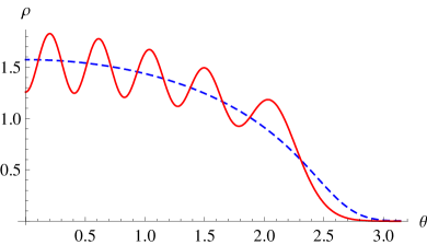
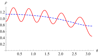
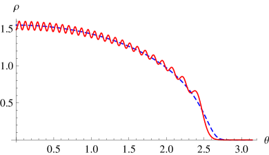
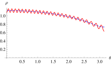
Figure 2: Plots of the densities $\rho_{N}^{\tt true}(\theta,t)$ (red, solid) and $\rho_{N}^{\tt sym}(\theta,T)$ (blue, dashed) for $t=2$ (left) and $t=5$ (right), $N=10$ (top), and $N=50$ (bottom).

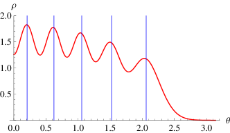
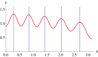
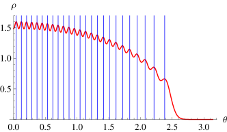
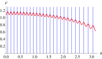
Figure 3: Plots of the density $\rho_{N}^{\tt true}(\theta,t)$ (oscillatory red curve) together with the positions of the angles of the zeros $\theta_{a}$ (vertical blue lines) for $t=2$ (left) and $t=5$ (right), $N=10$ (top), and $N=50$ (bottom).

4.2 asym zeros and true peaks

This comparison is shown in Figure 3. The main observation is that the locations of the delta functions of $\rho_{N}^{\tt asym}(\theta,\tau)$ approximate well the locations of the peaks in $\rho_{N}^{\tt true}(\theta,t)$. In this sense one can think about the $e^{i\theta_{j}}$ as the average eigenvalues of $W$.

5 Summary

The eigenvalues of non-self-intersecting Wilson loops in 2D YM have statistical properties related to exactly integrable systems. Several different exact finite-$N$ observables exist which approach in universal ways a common nonanalytic infinite-$N$ limit. One can interpret $\frac{1}{2N}$ as a viscosity [5, 7]. Thus the short-long distance crossover in large-$N$ YM in $\text{D}=2,3,4$ is mapped into the very small viscosity regime of “Burgers turbulence”.

6 Acknowledgments

We acknowledge support by BayEFG (RL), by the DOE under grant number DE-FG02-01ER41165 at Rutgers University (HN, RL), and by DFG and JSPS (TW). HN notes with regret that his research has for a long time been deliberately obstructed by his high energy colleagues at Rutgers.

References

- [1] R. Narayanan, H. Neuberger, JHEP03 (2006) 064.
- [2] R. Narayanan, H. Neuberger, JHEP12 (2007) 066.
- [3] B. Durhuus, P. Olesen, Nucl. Phys. B184 (1981) 461.
- [4] R. Lohmayer, H. Neuberger, T. Wettig, JHEP05 (2009) 107.
- [5] H. Neuberger, Phys. Lett. B666 (2008) 106.
- [6] J. M. Burgers, “The nonlinear diffusion equation: asymptotic solutions and statistical properties”, D. Reidel Publishing Company, 1974.
- [7] J.-P. Blaizot, M. A. Nowak, Phys. Rev. Lett. 101 (2008) 102001.
- [8] H. Neuberger, Phys. Lett. B670 (2008) 235.
- [9] P. Constantin, J. Wu, SIAM J. Math. Anal. 30 (1999) 937.