Electron-positron pairs in physics and astrophysics: from heavy nuclei to black holes
Abstract
Due to the interaction of physics and astrophysics we are witnessing in these years a splendid synthesis of theoretical, experimental and observational results originating from three fundamental physical processes. They were originally proposed by Dirac, by Breit and Wheeler and by Sauter, Heisenberg, Euler and Schwinger. For almost seventy years they have all three been followed by a continued effort of experimental verification on Earth-based experiments. The Dirac process, , has been by far the most successful. It has obtained extremely accurate experimental verification and has led as well to an enormous number of new physics in possibly one of the most fruitful experimental avenues by introduction of storage rings in Frascati and followed by the largest accelerators worldwide: DESY, SLAC etc. The Breit–Wheeler process, , although conceptually simple, being the inverse process of the Dirac one, has been by far one of the most difficult to be verified experimentally. Only recently, through the technology based on free electron X-ray laser and its numerous applications in Earth-based experiments, some first indications of its possible verification have been reached. The vacuum polarization process in strong electromagnetic field, pioneered by Sauter, Heisenberg, Euler and Schwinger, introduced the concept of critical electric field . It has been searched without success for more than forty years by heavy-ion collisions in many of the leading particle accelerators worldwide.
The novel situation today is that these same processes can be studied on a much more grandiose scale during the gravitational collapse leading to the formation of a black hole being observed in Gamma Ray Bursts (GRBs). This report is dedicated to the scientific race. The theoretical and experimental work developed in Earth-based laboratories is confronted with the theoretical interpretation of space-based observations of phenomena originating on cosmological scales. What has become clear in the last ten years is that all the three above mentioned processes, duly extended in the general relativistic framework, are necessary for the understanding of the physics of the gravitational collapse to a black hole. Vice versa, the natural arena where these processes can be observed in mutual interaction and on an unprecedented scale, is indeed the realm of relativistic astrophysics.
We systematically analyze the conceptual developments which have followed the basic work of Dirac and Breit–Wheeler. We also recall how the seminal work of Born and Infeld inspired the work by Sauter, Heisenberg and Euler on effective Lagrangian leading to the estimate of the rate for the process of electron–positron production in a constant electric field. In addition of reviewing the intuitive semi-classical treatment of quantum mechanical tunneling for describing the process of electron–positron production, we recall the calculations in Quantum Electro-Dynamics of the Schwinger rate and effective Lagrangian for constant electromagnetic fields. We also review the electron–positron production in both time-alternating electromagnetic fields, studied by Brezin, Itzykson, Popov, Nikishov and Narozhny, and the corresponding processes relevant for pair production at the focus of coherent laser beams as well as electron beam–laser collision. We finally report some current developments based on the general JWKB approach which allows to compute the Schwinger rate in spatially varying and time varying electromagnetic fields.
We also recall the pioneering work of Landau and Lifshitz, and Racah on the collision of charged particles as well as experimental success of AdA and ADONE in the production of electron–positron pairs.
We then turn to the possible experimental verification of these phenomena. We review: (A) the experimental verification of the process studied by Dirac. We also briefly recall the very successful experiments of annihilation to hadronic channels, in addition to the Dirac electromagnetic channel; (B) ongoing Earth based experiments to detect electron–positron production in strong fields by focusing coherent laser beams and by electron beam–laser collisions; and (C) the multiyear attempts to detect electron–positron production in Coulomb fields for a large atomic number in heavy ion collisions. These attempts follow the classical theoretical work of Popov and Zeldovich, and Greiner and their schools.
We then turn to astrophysics. We first review the basic work on the energetics and electrodynamical properties of an electromagnetic black hole and the application of the Schwinger formula around Kerr–Newman black holes as pioneered by Damour and Ruffini. We only focus on black hole masses larger than the critical mass of neutron stars, for convenience assumed to coincide with the Rhoades and Ruffini upper limit of 3.2 . In this case the electron Compton wavelength is much smaller than the spacetime curvature and all previous results invariantly expressed can be applied following well established rules of the equivalence principle. We derive the corresponding rate of electron–positron pair production and introduce the concept of dyadosphere. We review recent progress in describing the evolution of optically thick electron–positron plasma in presence of supercritical electric field, which is relevant both in astrophysics as well as ongoing laser beam experiments. In particular we review recent progress based on the Vlasov-Boltzmann-Maxwell equations to study the feedback of the created electron–positron pairs on the original constant electric field. We evidence the existence of plasma oscillations and its interaction with photons leading to energy and number equipartition of photons, electrons and positrons. We finally review the recent progress obtained by using the Boltzmann equations to study the evolution of an electron–positron-photon plasma towards thermal equilibrium and determination of its characteristic timescales. The crucial difference introduced by the correct evaluation of the role of two and three body collisions, direct and inverse, is especially evidenced. We then present some general conclusions.
The results reviewed in this report are going to be submitted to decisive tests in the forthcoming years both in physics and astrophysics. To mention only a few of the fundamental steps in testing in physics we recall the starting of experimental facilities at the National Ignition Facility at the Lawrence Livermore National Laboratory as well as corresponding French Laser the Mega Joule project. In astrophysics these results will be tested in galactic and extragalactic black holes observed in binary X-ray sources, active galactic nuclei, microquasars and in the process of gravitational collapse to a neutron star and also of two neutron stars to a black hole giving origin to GRBs. The astrophysical description of the stellar precursors and the initial physical conditions leading to a gravitational collapse process will be the subject of a forthcoming report. As of today no theoretical description has yet been found to explain either the emission of the remnant for supernova or the formation of a charged black hole for GRBs. Important current progress toward the understanding of such phenomena as well as of the electrodynamical structure of neutron stars, the supernova explosion and the theories of GRBs will be discussed in the above mentioned forthcoming report. What is important to recall at this stage is only that both the supernovae and GRBs processes are among the most energetic and transient phenomena ever observed in the Universe: a supernova can reach energy of ergs on a time scale of a few months and GRBs can have emission of up to ergs in a time scale as short as of a few seconds. The central role of neutron stars in the description of supernovae, as well as of black holes and the electron–positron plasma, in the description of GRBs, pioneered by one of us (RR) in 1975, are widely recognized. Only the theoretical basis to address these topics are discussed in the present report.
1 Introduction
The annihilation of electron–positron pair into two photons, and its inverse process – the production of electron–positron pair by the collision of two photons were first studied in the framework of quantum mechanics by P.A.M. Dirac and by G. Breit and J.A. Wheeler in the 1930s [1, 2].
A third fundamental process was pioneered by the work of Fritz Sauter and Oscar Klein, pointing to the possibility of creating an electron–positron pair from the vacuum in a constant electromagnetic field. This became known as the ‘Klein paradox’ and such a process named as vacuum polarization. It would occur for an electric field stronger than the critical value
| (1) |
where , , and are respectively the electron mass and charge, the speed of light and the Planck’s constant.
The experimental difficulties to verify the existence of such three processes became immediately clear. While the process studied by Dirac was almost immediately observed [3] and the electron–positron collisions became possibly the best tested and prolific phenomenon ever observed in physics. The Breit–Wheeler process, on the contrary, is still today waiting a direct observational verification. Similarly the vacuum polarization process defied dedicated attempts for almost fifty years in experiments in nuclear physics laboratories and accelerators all over the world, see Section 6.
From the theoretical point of view the conceptual changes implied by these processes became immediately clear. They were by vastness and depth only comparable to the modifications of the linear gravitational theory of Newton introduced by the nonlinear general relativistic equations of Einstein. In the work of Euler, Oppenheimer and Debye, Born and his school it became clear that the existence of the Breit–Wheeler process was conceptually modifying the linearity of the Maxwell theory. In fact the creation of the electron–positron pair out of the two photons modifies the concept of superposition of the linear electromagnetic Maxwell equations and impose the necessity to transit to a nonlinear theory of electrodynamics. In a certain sense the Breit–Wheeler process was having for electrodynamics the same fundamental role of Gedankenexperiment that the equivalence principle had for gravitation. Two different attempts to study these nonlinearities in the electrodynamics were made: one by Born and Infeld [4, 5, 6] and one by Euler and Heisenberg [7]. These works prepared the even greater revolution of Quantum Electro-Dynamics by Tomonaga [8], Feynman [9, 10, 11], Schwinger [12, 13, 14] and Dyson [15, 16].
In Section 2 we review the fundamental contributions to the electron–positron pair creation and annihilation and to the concept of the critical electric field. In Section 2.1 we review the Dirac derivation [1] of the electron–positron annihilation process obtained within the perturbation theory in the framework of relativistic quantum mechanics and his derivation of the classical formula for the cross-section in the rest frame of the electron
where is the energy of the positron and is as usual the fine structure constant, and we recall the corresponding formula for the center of mass reference frame. In Section 2.2 we recall the main steps in the classical Breit–Wheeler work [2] on the production of a real electron–positron pair in the collision of two photons, following the same method used by Dirac and leading to the evaluation of the total cross-section in the center of mass of the system
where is the reduced velocity of the electron or the positron. In Section 2.3 we recall the basic higher order processes, compared to the Dirac and Breit–Wheeler ones, leading to pair creation. In Section 2.4 we recall the famous Klein paradox [17, 18] and the possible tunneling between the positive and negative energy states leading to the concept of level crossing and pair creation by analogy to the Gamow tunneling [19] in the nuclear potential barrier. We then turn to the celebrated Sauter work [20] showing the possibility of creating a pair in a uniform electric field . We recover in Section 2.5.1 a JWKB approximation in order to reproduce and improve on the Sauter result by obtaining the classical Sauter exponential term as well as the prefactor
where for a spin- particle and for spin-, is the volume. Finally, in Section 2.5.2 the case of a simultaneous presence of an electric and a magnetic field is presented leading to the estimate of pair production rate
and
where
where the scalar and the pseudoscalar are
where is the dual field tensor.
In Section 3 we first recall the seminal work of Hans Euler [21] pointing out for the first time the necessity of nonlinear character of electromagnetism introducing the classical Euler Lagrangian
where
a first order perturbation to the Maxwell Lagrangian. In Section 3.2 we review the alternative theoretical approach of nonlinear electrodynamics by Max Born [5] and his collaborators, to the more ambitious attempt to obtain the correct nonlinear Lagrangian of Electro-Dynamics. The motivation of Born was to attempt a theory free of divergences in the observable properties of an elementary particle, what has become known as ‘unitarian’ standpoint versus the ‘dualistic’ standpoint in description of elementary particles and fields. We recall how the Born Lagrangian was formulated
and one of the first solutions derived by Born and Infeld [6]. We also recall one of the interesting aspects of the courageous approach of Born had been to formulate this Lagrangian within a unified theory of gravitation and electromagnetism following Einstein program. Indeed, we also recall the very interesting solution within the Born theory obtained by Hoffmann [22, 23]. Still in the work of Born [5] the seminal idea of describing the nonlinear vacuum properties of this novel electrodynamics by an effective dielectric constant and magnetic permeability functions of the field arisen. We then review in Section 3.3.1 the work of Heisenberg and Euler [7] adopting the general approach of Born and generalizing to the presence of a real and imaginary part of the electric permittivity and magnetic permeability. They obtain an integral expression of the effective Lagrangian given by
where are the dimensionless reduced fields in the unit of the critical field ,
obtaining the real part and the crucial imaginary term which relates to the pair production in a given electric field. It is shown how these results give as a special case the previous result obtained by Euler (78). In Section 3.3.2 the work by Weisskopf [24] working on a spin-0 field fulfilling the Klein–Gordon equation, in contrast to the spin 1/2 field studied by Heisenberg and Euler, confirms the Euler-Heisenberg result. Weisskopf obtains explicit expression of pair creation in an arbitrary strong magnetic field and in an electric field described by and expansion.
For the first time Heisenberg and Euler provided a description of the vacuum properties by the characteristic scale of strong field and the effective Lagrangian of nonlinear electromagnetic fields. In 1951, Schwinger [25, 26, 27] made an elegant quantum field theoretic reformulation of this discovery in the QED framework. This played an important role in understanding the properties of the QED theory in strong electromagnetic fields. The QED theory in strong coupling regime, i.e., in the regime of strong electromagnetic fields, is still a vast arena awaiting for experimental verification as well as of further theoretical understanding.
In Section 4 after recalling some general properties of QED in Section 4.1 and some basic processes in Section 4.2 we proceed to the consideration of the Dirac and the Breit–Wheeler processes in QED in Secton 4.3. Then we discuss some higher order processes, namely double pair production in Section 4.4, electron-nucleus bremsstrahlung and pair production by a photon in the field of a nucleus in Section 4.5, and finally pair production by two ions in Section 4.6. In Section 4.7 the classical result for the vacuum to vacuum decay via pair creation in uniform electric field by Schwinger is recalled
This formula generalizes and encompasses the previous results reviewed in our report: the JWKB results, discussed in Section 2.5, and the Sauter exponential factor (57), and the Heisenberg-Euler imaginary part of the effective Lagrangian. We then recall the generalization of this formula to the case of a constant electromagnetic fields. Such results were further generalized to spatially nonuniform and time-dependent electromagnetic fields by Nikishov [28], Vanyashin and Terent’ev [29], Popov [30, 31, 32], Narozhny and Nikishov [33] and Batalin and Fradkin [34]. We then conclude this argument by giving the real and imaginary parts for the effective Lagrangian for arbitrary constant electromagnetic field recently published by Ruffini and Xue [35]. This result generalizes the previous result obtained by Weisskopf in strong fields. In weak field it gives the Euler-Heisenberg effective Lagrangian. As we will see in the Section 6.2 much attention has been given experimentally to the creation of pairs in the rapidly changing electric fields. A fundamental contribution in this field studying pair production rates in an oscillating electric field was given by Brezin and Itzykson [36] and we recover in Section 4.8 their main results which apply both to the case of bosons and fermions. We recall how similar results were independently obtained two years later by Popov [37]. In Section 4.10 we recall an alternative physical process considering the quantum theory of the interaction of free electron with the field of a strong electromagnetic waves: an ultrarelativistic electron absorbs multiple photons and emits only a single photon in the reaction [38]:
This process appears to be of the great relevance as we will see in the next Section for the nonlinear effects originating from laser beam experiments. Particularly important appears to be the possibility outlined by Burke et al. [39] that the high-energy photon created in the first process propagates through the laser field, it interacts with laser photons to produce an electron–positron pair
We also refer to the papers by Narozhny and Popov [40, 41, 42, 43, 44, 45] studying the dependence of this process on the status of the polarization of the photons.
We point out the great relevance of departing from the case of the uniform electromagnetic field originally considered by Sauter, Heisenberg and Euler, and Schwinger. We also recall some of the classical works of Brezin and Itzykson and Popov on time varying fields. The space variation of the field was also considered in the classical papers of Nikishov and Narozhny as well as in the work of Wang and Wong. Finally, we recall the work of Khriplovich [46] studying the vacuum polarization around a Reissner–Nordström black hole. A more recent approach using the worldline formalism, sometimes called the string-inspired formalism, was advanced by Dunne and Schubert [47, 48].
In Section 5, after recalling studies of pair production in inhomogeneous electromagnetic fields in the literature by [48, 49, 50, 51, 52, 53], we present a brief review of our recent work [54] where the general formulas for pair production rate as functions of either crossing energy level or classical turning point, and total production rate are obtained in external electromagnetic fields which vary either in one space direction or in time . In Sections 5.1 and 5.2, these formulas are explicitly derived in the JWKB approximation and generalized to the case of three-dimensional electromagnetic configurations. We apply these formulas to several cases of such inhomogeneous electric field configurations, which are classified into two categories. In the first category, we study two cases: a semi-confined field for and the Sauter field
where is width in the -direction, and
In these two cases the pairs produced are not confined by the electric potential and can reach an infinite distance. The resultant pair production rate varies as a function of space coordinate. The result we obtained is drastically different from the Schwinger rate in homogeneous electric fields without any boundary. We clearly show that the approximate application of the Schwinger rate to electric fields limited within finite size of space overestimates the total number of pairs produced, particularly when the finite size is comparable with the Compton wavelength , see Figs. 7 and 8 where it is clearly shown how the rate of pair creation far from being constant goes to zero at both boundaries. The same situation is also found for the case of the semi-confined field for , see Eq. (327). In the second category, we study a linearly rising electric field , corresponding to a harmonic potential , see Figs. 6. In this case the energy spectra of bound states are discrete and thus energy crossing levels for tunneling are discrete. To obtain the total number of pairs created, using the general formulas for pair production rate, we need to sum over all discrete energy crossing levels, see Eq. (338), provided these energy levels are not occupied. Otherwise, the pair production would stop due to the Pauli principle.
In Section 6 we focus on the phenomenology of electron–positron pair creation and annihilation experiments. There are three different aspects which are examined: the verification of the process (2) initially studied by Dirac, the process (3) studied by Breit and Wheeler, and then the classical work of vacuum polarization process around a supercritical nucleus, following the Sauter, Euler, Heisenberg and Schwinger work. We first recall in Section 6.1 how the process (2) predicted by Dirac was almost immediately discovered by Klemperer [3]. Following this discovery the electron–positron collisions have become possibly the most prolific field of research in the domain of particle physics. The crucial step experimentally was the creation of the first electron–positron collider the “Anello d’Accumulazione” (AdA) was built by the theoretical proposal of Bruno Touschek in Frascati (Rome) in 1960 [55]. Following the success of AdA (luminosity /(cm2 sec), beam energy 0.25GeV), it was decided to build in the Frascati National Laboratory a storage ring of the same kind, Adone. Electron-positron colliders have been built and proposed for this purpose all over the world (CERN, SLAC, INP, DESY, KEK and IHEP). The aim here is just to recall the existence of this enormous field of research which appeared following the original Dirac idea. The main cross-sections (345) and (346) are recalled and the diagram (Fig. 11) summarizing this very great success of particle physics is presented. While the Dirac process (2) has been by far one of the most prolific in physics, the Breit–Wheeler process (3) has been one of the most elusive for direct observations. In Earth-bound experiments the major effort today is directed to evidence this phenomenon in very strong and coherent electromagnetic field in lasers. In this process collision of many photons may lead in the future to pair creation. This topic is discussed in Section 6.2. Alternative evidence for the Breit–Wheeler process can come from optically thick electron–positron plasma which may be created either in the future in Earth-bound experiments, or currently observed in astrophysics, see Section 9. One additional way to probe the existence of the Breit–Wheeler process is by establishing in astrophysics an upper limits to observable high-energy photons, as a function of distance, propagating in the Universe as pioneered by Nikishov [56], see Section 6.4. We then recall in Section 6.3 how the crucial experimental breakthrough came from the idea of John Madey [57] of self-amplified spontaneous emission in an undulator, which results when charges interact with the synchrotron radiation they emit [58]. Such X-ray free electron lasers have been constructed among others at DESY and SLAC and focus energy onto a small spot hopefully with the size of the X-ray laser wavelength nm [59], and obtain a very large electric field , much larger than those obtainable with any optical laser of the same power. This technique can be used to achieve a very strong electric field near to its critical value for observable electron–positron pair production in vacuum. No pair can be created by a single laser beam. It is then assumed that each X-ray laser pulse is split into two equal parts and recombined to form a standing wave with a frequency . We then recall how for a laser pulse with wavelength about and the theoretical diffraction limit being reached, the critical intensity laser beam would be
In Section 6.2.1 we recall the theoretical formula for the probability of pair production in time-alternating electric field in two limiting cases of large frequency and small frequency. It is interesting that in the limit of large field and small frequency the production rate approach the one of the Sauter, Heisenberg, Euler and Schwinger, discussed in Section 4. In the following Section 6.2.2 we recall the actually reached experimental limits quoted by Ringwald [60] for a X-ray laser and give a reference to the relevant literature. In Section 6.2.3 we summarize some of the most recent theoretical estimates for pair production by a circularly polarized laser beam by Narozhny, Popov and their collaborators. In this case the field invariants (69) are not vanishing and pair creation can be achieved by a single laser beam. They computed the total number of electron–positron pairs produced as a function of intensity and focusing parameter of the laser. Particularly interesting is their analysis of the case of two counter-propagating focused laser pulses with circular polarizations, pair production becomes experimentally observable when the laser intensity for each beam, which is about orders of magnitude lower than for a single focused laser pulse, and more than orders of magnitude lower than the critical intensity (351). Equally interesting are the considerations which first appear in treating this problem that the back reaction of the pairs created on the field has to be taken into due account. We give the essential references and we will see in Section 8 how indeed this feature becomes of paramount importance in the field of astrophysics. We finally review in Section 6.2.4 the technological situation attempting to increase both the frequency and the intensity of laser beams.
The difficulty of evidencing the Breit–Wheeler process even when the high-energy photon beams have a center of mass energy larger than the energy-threshold MeV was clearly recognized since the early days. We discuss the crucial role of the effective nonlinear terms originating in strong electromagnetic laser fields: the interaction needs not to be limited to initial states of two photons [61, 62]. A collective state of many interacting laser photons occurs. We turn then in Section 6.3 to an even more complex and interesting procedure: the interaction of an ultrarelativistic electron beam with a terawatt laser pulse, performed at SLAC [63], when strong electromagnetic fields are involved. A first nonlinear Compton scattering process occurs in which the ultrarelativistic electrons absorb multiple photons from the laser field and emit a single photon via the process (229). The theory of this process has been given in Section 4.10. The second is a drastically improved Breit–Wheeler process (230) by which the high-energy photon , created in the first process, propagates through the laser field and interacts with laser photons to produce an electron–positron pair [39]. In Section 6.3.1 we describe the status of this very exciting experiments which give the first evidence for the observation in the laboratory of the Breit–Wheeler process although in a somewhat indirect form. Having determined the theoretical basis as well as attempts to verify experimentally the Breit–Wheeler formula we turn in Section 6.4 to a most important application of the Breit–Wheeler process in the framework of cosmology. As pointed out by Nikishov [56] the existence of background photons in cosmology puts a stringent cutoff on the maximum trajectory of the high-energy photons in cosmology.
Having reviewed both the theoretical and observational evidence of the Dirac and Breit–Wheeler processes of creation and annihilation of electron–positron pairs we turn then to one of the most conspicuous field of theoretical and experimental physics dealing with the process of electron–positron pair creation by vacuum polarization in the field of a heavy nuclei. This topic has originated one of the vastest experimental and theoretical physics activities in the last forty years, especially by the process of collisions of heavy ions. We first review in Section 6.5 the catastrophe, a collapse to the center, in semi-classical approach, following the Pomeranchuk work [64] based on the imposing the quantum conditions on the classical treatment of the motion of two relativistic particles in circular orbits. We then proceed showing in Section 6.5.3 how the introduction of the finite size of the nucleus, following the classical work of Popov and Zeldovich [65], leads to the critical charge of a nucleus of above which a bare nucleus would lead to the level crossing between the bound state and negative energy states of electrons in the field of a bare nucleus. We then review in Section 6.5.5 the recent theoretical progress in analyzing the pair creation process in a Coulomb field, taking into account radial dependence and time variability of electric field. We finally recall in Section 6.6 the attempt to use heavy-ion collisions to form transient superheavy “quasimolecules”: a long-lived metastable nuclear complex with . It was expected that the two heavy ions of charges respectively and with would reach small inter-nuclear distances well within the electron’s orbiting radii. The electrons would not distinguish between the two nuclear centers and they would evolve as if they were bounded by nuclear “quasimolecules” with nuclear charge . Therefore, it was expected that electrons would evolve quasi-statically through a series of well defined nuclear “quasimolecules” states in the two-center field of the nuclei as the inter-nuclear separation decreases and then increases again. When heavy-ion collision occurs the two nuclei come into contact and some deep inelastic reaction occurs determining the duration of this contact. Such “sticking time” is expected to depend on the nuclei involved in the reaction and on the beam energy. Theoretical attempts have been proposed to study the nuclear aspects of heavy-ion collisions at energies very close to the Coulomb barrier and search for conditions, which would serve as a trigger for prolonged nuclear reaction times, to enhance the amplitude of pair production. The sticking time should be larger than sec [66] in order to have significant pair production. Up to now no success has been achieved in justifying theoretically such a long sticking time. In reality the characteristic sticking time has been found of the order of sec, hundred times shorter than the needed to activate the pair creation process. We finally recall in Section 6.6.2 the Darmstadt-Brookhaven dialogue between the Orange and the Epos groups and the Apex group at Argonne in which the claim for discovery of electron–positron pair creation by vacuum polarization in heavy-ion collisions was finally retracted. Out of the three fundamental processes addressed in this report, the Dirac electron–positron annihilation and the Breit–Wheeler electron–positron creation from two photons have found complete theoretical descriptions within Quantum Electro-Dynamics. The first one is very likely the best tested process in physical science, while the second has finally obtained the first indirect experimental evidence. The third process, the one of the vacuum polarization studied by Sauter, Euler, Heisenberg and Schwinger, presents in Earth-bound experiments presents a situation “terra incognita”.
We turn then to astrophysics, where, in the process of gravitational collapse to a black hole and in its outcomes these three processes will be for the first time verified on a much larger scale, involving particle numbers of the order of , seeing both the Dirac process and the Breit–Wheeler process at work in symbiotic form and electron–positron plasma created from the “blackholic energy” during the process of gravitational collapse. It is becoming more and more clear that the gravitational collapse process to a Kerr–Newman black hole is possibly the most complex problem ever addressed in physics and astrophysics. What is most important for this report is that it gives for the first time the opportunity to see the above three processes simultaneously at work under ultrarelativistic special and general relativistic regimes. The process of gravitational collapse is characterized by the timescale sec and the energy involved are of the order of ergs. It is clear that this is one of the most energetic and most transient phenomena in physics and astrophysics and needs for its correct description such a highly time varying treatment. Our approach in Section 7 is to gain understanding of this process by separating the different components and describing 1) the basic energetic process of an already formed black hole, 2) the vacuum polarization process of an already formed black hole, 3) the basic formula of the gravitational collapse recovering the Tolman-Oppenheimer-Snyder solutions and evolving to the gravitational collapse of charged and uncharged shells. This will allow among others to obtain a better understanding of the role of irreducible mass of the black hole and the maximum blackholic energy extractable from the gravitational collapse. We will as well address some conceptual issues between general relativity and thermodynamics which have been of interest to theoretical physicists in the last forty years. Of course in these brief chapter we will be only recalling some of these essential themes and refer to the literature where in-depth analysis can be found. In Section 7.1 we recall the Kerr–Newman metric and the associated electromagnetic field. We then recall the classical work of Carter [67] integrating the Hamilton-Jacobi equations for charged particle motions in the above given metric and electromagnetic field. We then recall in Section 7.2 the introduction of the effective potential techniques in order to obtain explicit expression for the trajectory of a particle in a Kerr–Newman geometry, and especially the introduction of the reversible–irreversible transformations which lead then to the Christodoulou-Ruffini mass formula of the black hole
where is the irreducible mass of a black hole, and are its charge and angular momentum. We then recall in Section 7.3 the positive and negative root states of the Hamilton–Jacobi equations as well as their quantum limit. We finally introduce in Section 7.4 the vacuum polarization process in the Kerr–Newman geometry as derived by Damour and Ruffini [68] by using a spatially orthonormal tetrad which made the application of the Schwinger formalism in this general relativistic treatment almost straightforward. We then recall in Section 7.5 the definition of a dyadosphere in a Reissner–Nordström geometry, a region extending from the horizon radius
out to an outer radius
where the dimensionless mass and charge parameters , . In Section 7.6 the definition of a dyadotorus in a Kerr–Newman metric is recalled. We have focused on the theoretically well defined problem of pair creation in the electric field of an already formed black hole. Having set the background for the blackholic energy we recall some fundamental features of the dynamical process of the gravitational collapse. In Section 7.7 we address some specific issues on the dynamical formation of the black hole, recalling first the Oppenheimer-Snyder solution [69] and then considering its generalization to the charged nonrotating case using the classical work of W. Israel and V. de la Cruz [70, 71]. In Section 7.7.1 we recover the classical Tolman-Oppenheimer-Snyder solution in a more transparent way than it is usually done in the literature. In the Section 7.7.2 we are studying using the Israel-de la Cruz formalism the collapse of a charged shell to a black hole for selected cases of a charged shell collapsing on itself or collapsing in an already formed Reissner–Nordström black hole. Such elegant and powerful formalism has allowed to obtain for the first time all the analytic equations for such large variety of possibilities of the process of the gravitational collapse. The theoretical analysis of the collapsing shell considered in the previous section allows to reach a deeper understanding of the mass formula of black holes at least in the case of a Reissner–Nordström black hole. This allows as well to give in Section 7.8 an expression of the irreducible mass of the black hole only in terms of its kinetic energy of the initial rest mass undergoing gravitational collapse and its gravitational energy and kinetic energy at the crossing of the black hole horizon
Similarly strong, in view of their generality, are the considerations in Section 7.8.2 which indicate a sharp difference between the vacuum polarization process in an overcritical and undercritical black hole. For the electron–positron plasma created will be optically thick with average particle energy 10 MeV. For the process of the radiation will be optically thin and the characteristic energy will be of the order of eV. This argument will be further developed in a forthcoming report. In Section 7.9 we show how the expression of the irreducible mass obtained in the previous Section leads to a theorem establishing an upper limit to 50% of the total mass energy initially at rest at infinity which can be extracted from any process of gravitational collapse independent of the details. These results also lead to some general considerations which have been sometimes claimed in reconciling general relativity and thermodynamics.
The conditions encountered in the vacuum polarization process around black holes lead to a number of electron–positron pairs created of the order of confined in the dyadosphere volume, of the order of a few hundred times to the horizon of the black hole. Under these conditions the plasma is expected to be optically thick and is very different from the nuclear collisions and laser case where pairs are very few and therefore optically thin. We turn then in Section 8, to discuss a new phenomenon: the plasma oscillations, following the dynamical evolution of pair production in an external electric field close to the critical value. In particular, we will examine: (i) the back reaction of pair production on the external electric field; (ii) the screening effect of pairs on the electric field; (iii) the motion of pairs and their interactions with the created photon fields. In Secs. 8.1 and 8.2, we review semi-classical and kinetic theories describing the plasma oscillations using respectively the Dirac-Maxwell equations and the Boltzmann-Vlasov equations. The electron–positron pairs, after they are created, coherently oscillate back and forth giving origin to an oscillating electric field. The oscillations last for at least a few hundred Compton times. We review the damping due to the quantum decoherence. The energy from collective motion of the classical electric field and pairs flows to the quantum fluctuations of these fields. This process is quantitatively discussed by using the quantum Boltzmann-Vlasov equation in Sections 8.4 and 8.5. The damping due to collision decoherence is quantitatively discussed in Sections 8.6 and 8.7 by using Boltzmann-Vlasov equation with particle collisions terms. This damping determines the energy flows from collective motion of the classical electric field and pairs to the kinetic energy of non-collective motion of particles of these fields due to collisions. In Section 8.7, we particularly address the study of the influence of the collision processes on the plasma oscillations in supercritical electric field [72]. It is shown that the plasma oscillation is mildly affected by a small number of photons creation in the early evolution during a few hundred Compton times (see Fig. 32). In the later evolution of Compton times, the oscillating electric field is damped to its critical value with a large number of photons created. An equipartition of number and energy between electron–positron pairs and photons is reached (see Fig. 32). In Section 8.8, we introduce an approach based on the following three equations: the number density continuity equation, the energy-momentum conservation equation and the Maxwell equations. We describe the plasma oscillation for both overcritical electric field and undercritical electric field [73]. In additional of reviewing the result well known in the literature for we review some novel result for the case . It was traditionally assumed that electron–positron pairs, created by the vacuum polarization process, move as charged particles in external uniform electric field reaching arbitrary large Lorentz factors. It is reviewed how recent computations show the existence of plasma oscillations of the electron–positron pairs also for . For both cases we quote the maximum Lorentz factors reached by the electrons and positrons as well as the length of oscillations. Two specific cases are given. For the length of oscillations 10 , and the length of oscillations 107 . We also review the asymptotic behavior in time, , of the plasma oscillations by the phase portrait technique. Finally we review some recent results which differentiate the case from the one with respect to the creation of the rest mass of the pair versus their kinetic energy. For the vacuum polarization process transforms the electromagnetic energy of the field mainly in the rest mass of pairs, with moderate contribution to their kinetic energy.
We then turn in Section 9 to the last physical process needed in ascertaining the reaching of equilibrium of an optically thick electron–positron plasma. The average energy of electrons and positrons we illustrate is MeV. These bounds are necessary from the one hand to have significant amount of electron–positron pairs to make the plasma optically thick, and from the other hand to avoid production of other particles such as muons. As we will see in the next report these are indeed the relevant parameters for the creation of ultrarelativistic regimes to be encountered in pair creation process during the formation phase of a black hole. We then review the problem of evolution of optically thick, nonequilibrium electron–positron plasma, towards an equilibrium state, following [74, 75]. These results have been mainly obtained by two of us (RR and GV) in recent publications and all relevant previous results are also reviewed in this Section 9. We have integrated directly relativistic Boltzmann equations with all binary and triple interactions between electrons, positrons and photons two kinds of equilibrium are found: kinetic and thermal ones. Kinetic equilibrium is obtained on a timescale of few , where and are Thomson’s cross-section and electron–positron concentrations respectively, when detailed balance is established between all binary interactions in plasma. Thermal equilibrium is reached on a timescale of few , when all binary and triple, direct and inverse interactions are balanced. In Section 9.1 basic plasma parameters are illustrated. The computational scheme as well as the discretization procedure are discussed in Section 9.2. Relevant conservation laws are given in Section 9.3. Details on binary interactions, consisting of Compton, Møller and Bhabha scatterings, Dirac pair annihilation and Breit–Wheeler pair creation processes, and triple interactions, consisting of relativistic bremsstrahlung, double Compton process, radiative pair production and three photon annihilation process, are presented in Section 9.5 and 9.6, respectively. In Section 9.5 collisional integrals with binary interactions are computed from first principles, using QED matrix elements. In Section 9.7 Coulomb scattering and the corresponding cutoff in collisional integrals are discussed. Numerical results are presented in Section 9.8 where the time dependence of energy and number densities as well as chemical potential and temperature of electron–positron-photon plasma is shown, together with particle spectra. The most interesting result of this analysis is to have differentiate the role of binary and triple interactions. The detailed balance in binary interactions following the classical work of Ehlers [76] leads to a distribution function of the form of the Fermi-Dirac for electron–positron pairs or of the Bose-Einstein for the photons. This is the reason we refer in the text to such conditions as the Ehlers equilibrium conditions. The crucial role of the direct and inverse three-body interactions is well summarized in fig. 41, panel A from which it is clear that the inverse three-body interactions are essential in reaching thermal equilibrium. If the latter are neglected, the system deflates to the creation of electron–positron pairs all the way down to the threshold of MeV. This last result which is referred as the Cavallo–Rees scenario [77] is simply due to improper neglection of the inverse triple reaction terms.
In Section 10 we present some general remarks.
Here and in the following we will use Latin indices running from 1 to 3, Greek indices running from 0 to 3, and we will adopt the Einstein summation rule.
2 The fundamental contributions to the electron–positron pair creation and annihilation and the concept of critical electric field
In this Section we recall the annihilation process of an electron–positron pair with the production of two photons
| (2) |
studied by Dirac in [1], the Breit–Wheeler process of electron–positron pair production by light-light collisions [2]
| (3) |
and the vacuum polarization in external electric field, introduced by Sauter [20]. These three results, obtained in the mid-30’s of the last century [78, 79], played a crucial role in the development of the Quantum Electro-Dynamics (QED).
2.1 Dirac’s electron–positron annihilation
Dirac had proposed his theory of the electron [80, 81] in the framework of relativistic quantum theory. Such a theory predicted the existence of positive and negative energy states. Only the positive energy states could correspond to the electrons. The negative energy states had to have a physical meaning since transitions were considered to be possible from positive to negative energy states. It was proposed by Dirac [81] that nearly all possible states of negative energy are occupied with just one electron in accordance with Pauli’s exclusion principle and that the unoccupied states, ‘holes’ in the negative energy states should be regarded as ‘positrons’111Actually initially [1, 81] Dirac believed that these ‘holes’ in negative energy spectrum describe protons, but later he realized that these holes represent particles with the same mass as of electron but with opposite charge, ‘anti-electrons’ [82]. The discovery of these anti-electrons was made by Anderson in 1932 [83] and named by him ‘positrons’ [84].. Historical review of this exciting discovery is given in [85].
Adopting his time-dependent perturbation theory [86] in the framework of relativistic Quantum Mechanics Dirac pointed out in [1] the necessity of the annihilation process of electron–positron pair into two photons (2). He considered an electron under the simultaneous influence of two incident beams of radiation, which induce transition of the electron to states of negative energy, then he calculated the transition probability per unit time, using the well established validity of the Einstein emission and absorption coefficients, which connect spontaneous and stimulated emission probabilities. He obtained the explicit expression of the cross-section of the annihilation process.
Such process is spontaneous, i.e. it occurs necessarily for any pair of electron and positron independently of their energy. The process does not need any previously existing radiation. The derivation of the cross-section, considering the stimulated emission process, was simplified by the fact that the electromagnetic field could be treated as an external classical perturbation and did not need to be quantized [87].
Dirac started from his wave equation [80] for the spinor field :
| (4) |
where and are electron’s mass and charge, is electromagnetic vector potential, and the matrices and are:
| (5) |
where and are respectively the Pauli’s and unit matrices. By choosing a gauge in which vanishes he obtained:
| (6) |
where and are respectively the frequencies of the two beams, and are the unit vectors in their direction of motion and and are the polarization vectors, the modulus of which are the amplitudes of the two beams.
Dirac solved Eq. (4) by a perturbation method, finding a solution of the form , where is the solution in the free case, and is the first order perturbation containing the field , or, explicitly . He then computed the explicit expression of the second order expansion term , which represents electrons that have made the double photon emission process and decay into negative energy states. He evaluated the transition amplitude for the stimulated transition process, which reads
| (7) |
where , and are the photons’ frequencies and
| (8) |
is a dimensionless number depending on the unit vectors in the directions of the two photon’s polarization vectors and . The quantities and are respectively given by . Introducing the intensity of the two incident beams
| (9) |
where . Dirac obtained from the above transition amplitude the transition probability
| (10) |
In order to evaluate the spontaneous emission probability Dirac uses the relation between the Einstein coefficients and which is of the form
| (11) |
Integrating on all possible directions of emission he obtains the total probability per unit time in the rest frame of the electron
| (12) |
where is the energy of the positron and is the fine structure constant. Again, historically Dirac was initially confused about the negative energy states interpretation as we recalled. Although he derived the correct formula, he was doubtful about the presence in it of the mass of the electron or of the mass of the proton. Of course today this has been clarified and this derivation is fully correct if one uses the mass of the electron and applied this formula to description of electron–positron annihilation. The limit for high-energy pairs () is
| (13) |
The corresponding center of mass formula is
| (14) |
where is the reduced velocity of the electron or the positron.
2.2 Breit–Wheeler pair production
We now turn to the equally important derivation on the production of an electron–positron pair in the collision of two real photons given by Breit and Wheeler [2]. According to Dirac’s theory of the electron, this process is caused by a transition of an electron from a negative energy state to a positive energy under the influence of two light quanta on the vacuum. This process differently from the one considered by Dirac, which occurs spontaneously, has a threshold due to the fact that electron and positron mass is not zero. In other words in the center of mass of the system there must be sufficient available energy to create an electron–positron pair. This energy must be larger than twice of electron rest mass energy.
Breit and Wheeler, following the discovery of the positron by Anderson [84], studied the effect of two light waves upon an electron in a negative energy state, represented by a normalized Dirac wave function . Like in the previous case studied by Dirac [1] the light waves have frequencies , wave vectors and vector potentials (6). Under the influence of the light waves, the initial electron wave function is changed after some time into a final wave function . The method adopted is the time-dependent perturbation [86] (for details see [88]) to solve the Dirac equation with the time-dependent potential (6). The transition amplitude was calculated by an expansion in powers of up to . The wave function contains a term representing an electron in a positive energy state. The associated density is found to be
| (15) | ||||
| (16) |
where is the dimensionless number already obtained by Dirac, Eq. (8), depending on initial momenta and spin of the wave function and the polarizations of the quanta. This quantity is actually the squared transition matrix in the momenta and spin of initial and final states of light and electron–positron. The squared amplitudes in Eq. (15) are determined by the intensities of the two light beams as
| (17) |
The quantity in Eq. (15) is the difference in energies between initial light states and final electron–positron states. Indicating by , where is the four-momentum of the positron, the negative energy of the electron in its initial state and the corresponding quantity for the electron , where is the 4-momentum of the electron, is given by
| (18) |
and is the final momentum of the electron. From this energy and momentum conservation it follows
| (19) |
It is then possible to sum the probability densities (15) over all possible initial electron states of negative energy in the volume . An integral over the phase space must be performed. The effective collision area for the head-on collision of two light quanta was shown by Breit and Wheeler to be
| (20) |
where is the solid angler, which fulfills the total energy conservation .
In the center of mass of the system, the momenta of the electron and the positron are equal and opposite . In that frame the momenta of the photons in the initial state are . As a consequence, the energies of the electron and the positron are equal: , and so are the energies of the photons: . The total cross-section of the process is then
| (21) |
where , and . Therefore, the necessary kinematic condition in order for the process (3) taking place is that the energy of the two colliding photons be larger than the threshold , i.e.,
| (22) |
From Eq. (21) the total cross-section in the center of mass of the system is
| (23) |
In modern QED cross-sections (13) and (23) emerge form two tree-level Feynman diagrams (see, for example, the textbook [89] and Section 4).
For , the total effective cross-section is approximately proportional to
| (24) |
The cross-section in line (23) can be easily generalized to an arbitrary reference frame, in which the two photons and cross with arbitrary relative directions. The Lorentz invariance of the scalar product of their 4-momenta gives . Since , to obtain the total cross-section in the arbitrary frame , we must therefore make the following substitution [90]
| (25) |
in Eq. (23).
2.3 Collisional pair creation near nuclei: Bethe and Heitler, Landau and Lifshitz, Sauter, and Racah
After having recalled in the previous sections the classical works of Dirac on the reaction (2) and Breit–Wheeler on the reaction (3) it is appropriate to return for a moment on the discovery of electron–positron pairs from observations of cosmic rays. The history of this discovery sees as major actors on one side Carl Anderson [84] at Caltech and on the other side Patrick Maynard Stuart Blackett and Giuseppe Occhialini [91] at the Cavendish laboratory. A fascinating reconstruction of their work can be found e.g. in [85]. The scene was however profoundly influenced by a fierce conceptual battle between Robert A. Millikan at Caltech and Arthur Compton at Chicago on the mechanism of production of these cosmic rays. For a refreshing memory of these heated discussions and a role also of Sir James Hopwood Jeans see e.g. [92]. The contention by Millikan was that the electron–positron pairs had to come from photons originating between the stars, while Jeans located their source on the stars. Compton on the contrary insisted on their origin from the collision of charged particles in the Earth atmosphere. Moreover, at the same time there were indications that similar process of charged particles would occur by the scattering of the radiation from polonium-beryllium, see e.g. Joliot and Curie [93].
It was therefore a natural outcome that out of this scenario two major theoretical developments occurred. One development inquired electron–positron pair creation by the interaction of photons with nuclei following the reaction:
| (26) |
major contributors were Oppenheimer and Plesset [94], Heitler [95], Bethe-Heitler [96], Sauter [97] and Racah [98]. Heitler [95] obtained an order of magnitude estimate of the total cross-section of this process
| (27) |
In the ultrarelativistic case the total cross-section for pair production by a photon with a given energy is [96]
| (28) |
The second development was the study of the reaction
| (29) |
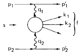
with the fundamental contribution of Landau and Lifshitz [99] and Racah [98, 100]. This process is an example of two photon pair production, see. Fig. 1. The 4-momenta of particles and are respectively and .
The total pair production cross-section is [99]
| (30) |
where . Racah [100] gives next to leading terms
| (31) |
The differential cross-section is given in Section 4.5. The differential distributions of electrons and positrons in a wide energy range was computed by Bhabha in [102].
In parallel progress on the reaction
| (32) |
was made by Sommerfeld [103], Heitler [95] and later by Bethe and Heitler [96].
Once the exact cross-section of the process (26) was known, the corresponding cross-section for the process (32) was found by an elegant method, called the equivalent photons method [101, 104]. The idea to treat the field of a fast charged particle in a way similar to electromagnetic radiation with particular frequency spectrum goes back to Fermi [105]. In such a way electromagnetic interaction of this particle e.g. with a nucleus is reduced to the interaction of this radiation with the nucleus. This idea was successfully applied to the calculation of the cross-section of interaction of relativistic charged particles by Weizsäcker [106] and Williams [107]. In fact, this method establishes the relation between the high-energy photon induced cross-section to the corresponding cross-section induced by a charged particle by the relation which is expressed by
| (33) |
where is the spectrum of equivalent photons. Its simple generalization,
| (34) |
Generally speaking, the equivalent photon approximation consists in ignoring that in such a case intermediate (virtual) photons are a) off mass shell and b) no longer transversely polarized. In the early years this spectrum was estimated on the ground of semi-classical approximations [106, 108] as
| (35) |
where is relativistic charged particle energy. This logarithmic dependence of the equivalent photon spectrum on the particle energy is characteristic of the Coulomb field. Racah [98] applied this method to compute the bremsstrahlung cross-section in the process (32), which is given in Section 4.5. Bethe and Heitler [96], obtained the same formula and computed the effect of the screening of the electrons of the nucleus. They found the screening is significant when the energy of relativistic particle is not too high (), where is the mass of the particle. Finally, Bethe and Heitler discussed the energy loss of charged particles in a medium.
Racah [100] used the equivalent photons method to compute from (34) the cross-section of pair creation at collision of two charged particles (29). Unlike Landau and Lifshitz result [99] which is valid only for the cross-section of Racah contains more terms of different powers of the logarithm, see Section 4.6.
2.4 Klein paradox and Sauter work
Every relativistic wave equation of a free particle of mass , momentum and energy , admits “positive energy” and “negative energy” solutions. In Minkowski space such a solution is symmetric with respect to the zero energy and the wave function given by
| (36) |
describes a relativistic particle, whose energy, mass and momentum satisfy,
| (37) |
This gives rise to the familiar positive and negative energy spectrum () of positive and negative energy states of the relativistic particle, as represented in Fig. 2. In such a situation, in absence of external field and at zero temperature, all the quantum states are stable; that is, there is no possibility of “positive” (“negative”) energy states decaying into “negative” (“positive”) energy states since there is an energy gap separating the negative energy spectrum from the positive energy spectrum. This stability condition was implemented by Dirac by considering all negative energy states as fully filled.
A scalar field described by the wave function satisfies the Klein–Gordon equation [109, 110, 111, 112]
| (38) |
If there is only an electric field in the -direction and varying only as a function of , we can choose a vector potential with the only nonzero component and potential energy
| (39) |
For an electron of charge by assuming
with a fixed transverse momentum in the -direction and an energy eigenvalue , and Eq. (38) becomes simply
| (40) |
Klein studied a relativistic particle moving in an external step function potential and in this case Eq. (40) is modified as
| (41) |
where . He solved his relativistic wave equation [109, 110, 111, 112] by considering an incident free relativistic wave of positive energy states scattered by the constant potential , leading to reflected and transmitted waves. He found a paradox that in the case , the reflected flux is larger than the incident flux , although the total flux is conserved, i.e. . This is known as the Klein paradox [17, 18]. This implies that negative energy states have contributions to both the transmitted flux and reflected flux .
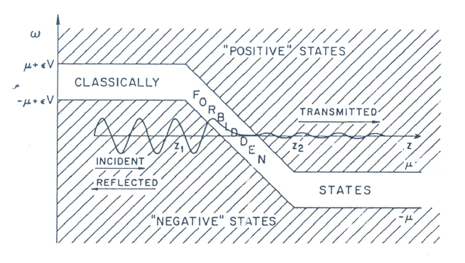
Sauter studied this problem by considering a potential varying in the -direction corresponding to a constant electric field in the -direction and considering spin 1/2 particles fulfilling the Dirac equation. In this case the energy is shifted by the amount . He further assumed an electric field uniform between and and null outside. Fig. 3 represents the corresponding sketch of allowed states. The key point now, which is the essence of the Klein paradox [17, 18], is that a level crossing between the positive and negative energy levels occurs. Under this condition the above mentioned stability of the “positive energy” states is lost for sufficiently strong electric fields. The same is true for “negative energy” states. Some “positive energy” and “negative energy” states have the same energy levels. Thus, these “negative energy” waves incident from the left will be both reflected back by the electric field and partly transmitted to the right as a “‘positive energy” wave, as shown in Fig. 3 [113]. This transmission represents a quantum tunneling of the wave function through the electric potential barrier, where classical states are forbidden. This quantum tunneling phenomenon was pioneered by George Gamow by the analysis of alpha particle emission or capture in the nuclear potential barrier (Gamow wall) [19]. In the latter case however the tunneling occurred between two states of positive energy while in the Klein paradox and Sauter computation the tunneling occurs for the first time between the positive and negative energy states giving rise to the totally new concept of the creation of particle-antiparticle pairs in the positive energy state as we are going to show.
Sauter first solved the relativistic Dirac equation in the presence of the constant electric field by the ansatz,
| (42) |
where spinor function obeys the following equation ( are Dirac matrices)
| (43) |
and the solution can be expressed in terms of hypergeometric functions [20]. Using this wave function (42) and the flux , Sauter computed the transmitted flux of positive energy states, the incident and reflected fluxes of negative energy states, as well as exponential decaying flux of classically forbidden states, as indicated in Fig. 3. Using the regular matching conditions of the wave functions and fluxes at boundaries of the potential, Sauter found that the transmission coefficient of the wave through the electric potential barrier from the negative energy state to positive energy states:
| (44) |
This is the probability of negative energy states decaying to positive energy states, caused by an external electric field. The method that Sauter adopted to calculate the transmission coefficient is indeed the same as the one Gamow used to calculate quantum tunneling of the wave function through nuclear potential barrier, leading to the -particle emission [19].
The simplest way to calculate the transmission coefficient (44) is the JWKB (Jeffreys–Wentzel–Kramers–Brillouin) approximation. The electric potential is not a constant. The corresponding solution of the Dirac equation is not straightforward, however it can be found using the quasi-classical, JWKB approximation. Particle’s energy , momentum and mass satisfy,
| (45) |
where the momentum is spatially dependent. The momentum for both negative and positive energy states and the wave functions exhibit usual oscillatory behavior of propagating wave in the -direction, i.e. . Inside the electric potential barrier where are the classically forbidden states, the momentum given by Eq. (45) becomes negative, and becomes imaginary, which means that the wave function will have an exponential behavior, i.e. , instead of the oscillatory behavior which characterizes the positive and negative energy states. Therefore the transmission coefficient of the wave through the one-dimensional potential barrier is given by
| (46) |
where and are roots of the equation defining the turning points of the classical trajectory, separating positive and negative energy states.
2.5 A semi-classical description of pair production in quantum mechanics
2.5.1 An external constant electric field
The phenomenon of pair production can be understood as a quantum mechanical tunneling process of relativistic particles. The external electric field modifies the positive and negative energy spectrum of the free Hamiltonian. Let the field vector point in the -direction. The electric potential is where and the length , then the positive and negative continuum energy spectra are
| (47) |
where is the momentum in -direction, transverse momenta. The energy spectra (47) are sketched in Fig. 4. One finds that crossing energy levels between two energy spectra and (47) appear, then quantum tunneling process occurs. The probability amplitude for this process can be estimated by a semi-classical calculation using JWKB method (see e.g. [88, 54]):
| (48) |
where
| (49) |
is the classical momentum. The limits of integration are the turning points of the classical orbit in imaginary time. They are determined by setting in Eq. (47). The solutions are
| (50) |
At the turning points of the classical orbit, the crossing energy level
| (51) |
as shown by dashed line in Fig. 4. The tunneling length is
| (52) |
which is independent of crossing energy levels . The critical electric field in Eq. (1) is the field at which the tunneling length (52) is twice the Compton length .
Changing the variable of integration from to ,
| (53) |
we obtain
| (54) |
and the JWKB probability amplitude (48) becomes
| (55) | |||||
Summing over initial and final spin states and integrating over the transverse phase space yields the final result
| (56) | |||||
where the transverse surface . For the constant electric field in , crossing energy levels vary from the maximal energy potential to the minimal energy potential . This probability Eq. (56) is independent of crossing energy levels . We integrate Eq. (56) over crossing energy levels and divide it by the time interval during which quantum tunneling occurs, and find the transition rate per unit time and volume
| (57) |
where for a spin- particle and for spin-, is the volume. The JWKB result contains the Sauter exponential [20] and reproduces as well the prefactor of Heisenberg and Euler [7].
Let us specify a quantitative condition for the validity of the above “semi-classical” JWKB approximation, which is in fact leading term of the expansion of wave function in powers of . In order to have the next-leading term be much smaller than the leading term, the de Broglie wavelength of wave function of the tunneling particle must have only small spatial variations [88]:
| (58) |
with of Eq. (49). The electric potential must satisfy
| (59) |
so that the result (57) is valid only for .
2.5.2 An additional constant magnetic field
The result (57) can be generalized to include a uniform magnetic field . The calculation is simplest by going into a Lorentz frame in which and are parallel to each other, which is always possible for uniform and static electromagnetic field. This frame will be referred to a center-of-fields frame, and the associated fields will be denoted by and . Suppose the initial and are not parallel, then we perform a Lorentz transformation with a velocity determined by [114]
| (60) |
in the direction as follows
| (61) | |||||
| (62) |
The fields and are now parallel. As a consequence, the wave function factorizes into a Landau state and into a spinor function, this last one first calculated by Sauter (see Eqs. (42),(43)). The energy spectrum in the JWKB approximation is still given by Eq. (47), but the squared transverse momenta is quantized due to the presence of the magnetic field: they are replaced by the Landau energy levels whose transverse energies have the discrete spectrum
| (63) |
where is the anomalous magnetic moment of the electron [115, 11, 116, 117, 118], the Landau frequency, for a spin- particle ( for a spin- particle) are eigenvalues of spinor operator in the -direction, i.e., in the common direction of and in the selected frame. The quantum number characterizing the Landau levels is associated with harmonic oscillations in the plane orthogonal to and . Apart from the replacement (63), the JWKB calculation remains the same as in the case of constant electric field (57). We must only replace the integration over the transverse phase space in Eq. (56) by the sum over all Landau levels with the degeneracy [88]:
| (64) |
The results are
| (65) |
and
| (66) |
We find the pair production rate per unit time and volume
| (67) |
and
| (68) |
We can now go back to an arbitrary Lorentz frame by expressing the result in terms of the two Lorentz invariants that can be formed from the and fields: the scalar and the pseudoscalar
| (69) |
where is the dual field tensor. We define the invariants and as the solutions of the invariant equations
| (70) |
and obtain
| (71) | |||||
| (72) |
In the special frame with parallel and , we see that and , so that we can replace (67) and (68) directly by the invariant expressions
| (73) |
and
| (74) |
which are pair production rates in arbitrary constant electromagnetic fields. We would like to point out that and in (69) are identically zero for any field configuration in which
| (75) |
As example, for a plane wave of electromagnetic field, and no pairs are produced.
3 Nonlinear electrodynamics and rate of pair creation
3.1 Hans Euler and light-light scattering
Hans Euler in his celebrated diplom thesis [21] discussed at the University of Leipzig called attention on the reaction
He recalled that Halpern [119] and Debye [120] first recognized that Dirac theory of electrons and the Dirac process (2) and the Breit–Wheeler one (3) had fundamental implication for the light on light scattering and consequently implied a modifications of the Maxwell equations.
If the energy of the photons is high enough then a real electron–positron pair is created, following Breit and Wheeler [2]. Again, if electron–positron pair does exist, two photons are created following [1]. In the case that the sum of energies of the two photons are smaller than the threshold then the reaction (above) still occurs through a virtual pair of electron and positron.
Under this condition the light-light scattering implies deviation from superposition principle, and therefore the linear theory of electromagnetism has to be substituted by a nonlinear one. Maxwell equations acquire nonlinear corrections due to the Dirac theory of the electron.
Euler first attempted to describe this nonlinearity by an effective Lagrangian representing the interaction term. He showed that the interaction term had to contain the forth power of the field strengths and its derivatives
| (76) |
being symbolically the electromagnetic field strength. He also estimated that the constants may be determined from dimensional considerations. Since the interaction has the dimension of energy density and contains electric charge in the forth power, the constants up to numerical factors are
| (77) |
where , namely “the field strength at the edge of the electron”.
From these general qualitative considerations Euler made an important further step taking into account that the Lagrangian (76) describing such a process had necessarily be built from invariants constructed from the field strengths, such as and following a precise procedure indicated by Max Born, see e.g. Pauli’s book [121]. Contrary to the usual Maxwell Lagrangian which is only a function of Euler first recognized that virtual electron–positron loops are represented by higher powers in the field strength corrections to the linear action of electromagnetism and written down the Lagrangian with second order corrections
| (78) |
where
| (79) |
The crucial result of Euler has been to determine the values of the coefficients (79) using time-dependent perturbation technique, e.g. [88] in Dirac theory.
Euler computed only the lowest order corrections in to Maxwell equations, namely “the 1/137 fraction of the field strength at the edge of the electron”. This perturbation method did not allow calculation of the tunneling rate for electron–positron pair creation in strong electromagnetic field which became the topic of the further work with Heisenberg [7].
3.2 Born’s nonlinear electromagnetism
A nonlinear theory of electrodynamics was independently proposed and developed by Max Born [4, 5] and later by Born and Infeld [6]. The main motivation in Born’s approach was the avoidance of infinities in an elementary particle description. Among the classical discussions on the fundamental interactions this topic had attracted attention of a large number of scientists. It was clear in fact from the considerations of J.J. Thomson, Abraham Lorentz that a point-like electron needed to have necessarily an infinite mass. The existence of a finite radius was attempted by Poincare by introduction of non-electromagnetic stresses. Also among the attempts we have to recall the theory of Mie [122, 123, 124, 125] modifying the Maxwell theory by nonlinear terms. This theory however had serious difficulty because solutions of Mie field equations depend on the absolute value of the potentials.
Max Born developed his theory in collaboration with Infeld. This alternative to the Maxwell theory is today called the Born-Infeld theory which still finds interest in the framework of subnuclear physics. The coauthorship of Infeld is felt by the general premise of the article in distinguishing the unitarian standpoint versus the dualistic standpoint in the description of particles and fields. “In the dualistic standpoint the particles are the sources of the field, are acted own by the field but are not a part of the field. Their characteristic properties are inertia, measured by specific constant, the mass” [6]. The unitarian theory developed by Thomson, Lorentz and Mie tends to describe the particle as a point-like singularity but with finite mass-energy density fulfilling uniquely an appropriate nonlinear field equations. It is interesting that this approach was later developed in the classical book by Einstein and Infeld [126] as well as in the classical paper by Einstein, Infeld and Hoffmann [127] on equations of motion in General Relativity.
In the Born-Infeld approach the emphasis is directed to a formalism encompassing General Relativity. But for simplicity the field equations are solved within the realm only of the electromagnetic field. A basic tensor is introduced. Its symmetric part is identified with a metric component and the antisymmetric part with the electromagnetic field. Formally therefore both the electromagnetic and gravitational fields are present although the authors explicitly avoided to insert the part of the Lagrangian describing the gravitational interaction and focused uniquely on the following nonlinear Lagrangian
| (80) |
The necessity to have the quadratic form of the term is due to obtain a Lagrangian invariant under reflections as pointed out by W. Pauli in his classical book [121]. For small field strengths Lagrangian (80) has the same form as (78) obtained by Euler.
From the nonlinear Lagrangian (80) Born and Infeld calculated the fields D and H through a tensor, and , where
| (81) |
and introduced therefore an effective electric permittivity and magnetic permeability which are functions of and . It is very interesting that Born and Infeld managed to obtain a solution for electrostatic field of a point particle () in which the radial component becomes infinite as but the radial component of E field is perfectly finite and is given by the expression
| (82) |
where is the “radius” of the electron.
Most important the integral of the electromagnetic energy is finite and given by
| (83) |
Equating this energy to they obtain .
The attempt therefore is to have a theoretical framework explaining the mass of the electron solely by a modified nonlinear electromagnetic field theory. This approach has not been followed by the current theories in particle physics where the dualistic approach is today adopted in which the charged particles are described by half-integer spin fields and electro-magnetic interactions by integer-spin fields.
The initial goal to develop a fully covariant theory of electrodynamics within General Relativity although not developed by Born himself was not abandoned. Hoffmann found an analytic solution [22] to the coupled system of the Einstein-Born-Infeld equations.
3.3 The Euler-Heisenberg Lagrangian
The two different approaches of Born and Infeld and of Euler present strong analogies and substantial differences. The attempt of Born and Infeld was to obtain at once a new nonlinear Lagrangian for electromagnetic field replacing the Maxwell Lagrangian in order to avoid the appearance of infinite self-energy for a classical point-like electron.
The attempt of Euler [128] was more conservative, to obtain the first order nonlinear perturbation corrections to the Maxwell Lagrangian on the ground of the Dirac theory of the electron.
Born and Infeld in addition introduced an effective dielectric constant and an effective magnetic permeability of the vacuum out of their nonlinear Lagrangian (80). This approach was adopted as well in the classical work of Heisenberg and Euler [7]. They introduced an effective Lagrangian on the ground of the Dirac theory of the electron and expressed the result in integral form duly taking away infinities, see Section 3.3.1. This integral was explicitly performed in the weak field limit and the special attention was given to the real part, see Section 3.3.2 and the imaginary part, see Section 3.3.3.
A successive work of Weisskopf [24] derived the same equations of Heisenberg and Euler for the real part of the dielectric constant and magnetic permeability by using instead of the spin 1/2 particle of the Dirac equation the scalar relativistic wave equation of Klein and Gordon. The results differ from the one of spin 1/2 particle only by a factor 2 due to the Bose statistics, see Section 3.3.1. The technique used by Weisskopf refers to the case of magnetic field of arbitrary strengths and describes the electric field perturbatively, see Section 3.3.2. As we will see in the following, the Heisenberg and Euler integral can be found in the case of arbitrary large both electric and magnetic fields, see Section 4.7.3.
3.3.1 Real part of the effective Lagrangian
We now recall how Heisenberg and Euler adopted the crucial idea of Max Born to describe the nonlinear Lagrangian by the introduction of an effective dielectric constant and magnetic permeability [7]. They further extended this idea by adopting the most general case of a dielectric constant containing real and imaginary part. Such an approach is generally followed in the description of dissipative media. The crucial point was to relate electron–positron pair creation process to imaginary part of the Lagrangian.
Let to be the Lagrangian density of electromagnetic fields , a Legendre transformation produces the Hamiltonian density:
| (84) |
In Maxwell’s theory, the two densities are given by
| (85) |
To quantitatively describe nonlinear electromagnetic properties of the vacuum based on the Dirac theory, Heisenberg and Euler introduced an effective Lagrangian of the vacuum state and an associated Hamiltonian density
| (86) |
Here and are complex functions of and . In Maxwell’s theory, in the vacuum, so that and .
Heisenberg and Euler derived the induced fields as the derivatives
| (87) |
Consequently, the vacuum behaves as a dielectric and permeable medium [7, 24] in which,
| (88) |
where and are complex and field-dependent dielectric and permeability tensors of the vacuum.
The discussions on complex dielectric and permeability tensors ( and ) can be found for example in Ref. [129]. The effective Lagrangian and Hamiltonian densities in such a medium are given by
| (89) |
In this medium, the conservation of electromagnetic energy has the form
| (90) |
where is the Poynting vector describing the density of electromagnetic energy flux. Consider complex and monochromatic electromagnetic field
| (91) |
of frequency , and dielectric and permeability tensors are frequency-dependent, i.e., and . Substituting these fields and tensors into the right-hand side of Eq. (90), one obtains the dissipation of electromagnetic energy per unit time into the medium
| (92) |
This is nonzero if and contain an imaginary part. The dissipation of electromagnetic energy in a medium is accompanied by heat production. In the light of the third thermodynamical law of entropy increase, the energy lost of electromagnetic fields in the medium is always positive, i.e., . As a consequence, and . The real parts of and represent an electric and magnetic polarizability of the vacuum and leads, for example, to the refraction of light in an electromagnetic field, or to the elastic scattering of light from light. The is the reflection index of the medium. The field dependence of and implies nonlinear electromagnetic properties of the vacuum as a dielectric and permeable medium.
The effective Lagrangian density (86) is a relativistically invariant function of the field strengths and . Since and are relativistic invariants, one can formally expand in powers of weak field strengths:
| (93) |
where are field-independent constants whose subscripts indicate the powers of and , respectively. Note that the invariant appears only in even powers since it is odd under parity and electromagnetism is parity invariant. The Lagrangian density (93) corresponds, via relation (84), to
| (94) | |||||
To obtain in Dirac’s theory, one has to calculate
| (95) |
where are the wave functions of the occupied negative energy states. When performing the sum, one encounters infinities which were removed by Dirac, Heisenberg, and Weisskopf [24, 130, 131, 132] by a suitable subtraction.
Heisenberg [131] expressed the Hamiltonian density in terms of the density matrix [130]. Heisenberg and Euler [7] calculated the coefficients . They did so by solving the Dirac equation in the presence of parallel electric and magnetic fields and in a specific direction,
| (96) |
where are the Landau states222Landau determined the quantum states of a particle in an external magnetic field in 1930 [88, 90]. depending on the magnetic field and are the spinor functions calculated by Sauter [20]. Heisenberg and Euler used the Euler-Maclaurin formula to perform the sum over , and obtained for the additional Lagrangian in (86) the integral representation
| (97) | |||||
where are the dimensionless reduced fields in the unit of the critical field ,
| (98) |
Expanding this expression in powers of up to yields the following values for the four constants:
| (99) |
The above results will receive higher corrections in QED and are correct only up to order . Up to this order, the field-dependent dielectric and permeability tensors and (88) have the following real parts for weak fields
| (100) |
3.3.2 Weisskopf effective Lagrangian
Weisskopf [24] adopted a simpler method. He considered first the special case in which and used the Landau states to find of Eq. (94), extracting from this and . Then he added a weak electric field to calculate perturbatively its contributions to in the Born approximation (see for example [88]). This led again to the coefficients (99), (100). In addition to the weak field expansion of real part of effective Lagrangian, Weisskopf also obtained the leading order term considering very large field strengths or ,
| (101) |
We shall address this same problem in Section 4.7.3 in the framework of QED [35] and we will compare and contrast our exact expressions with the one given by Weisskopf. The crucial point stressed by Weisskopf is that if one limits to the analysis of the real part of the dielectric constant and magnetic permeability then the nonlinearity of effective electromagnetic Lagrangian represent only small corrections even for field strengths which are much higher than the critical field strength . As we will show however, the contribution of the imaginary part of the effective Lagrangian diverges as pointed out by Heisenberg and Euler [7].
3.3.3 Imaginary part of the effective Lagrangian
Heisenberg and Euler [7] were the first to realize that for the powers series expansion (93) is not convergent, due to singularities of the integrand in (97) at . They concluded that the powers series expansion (93) does not yield all corrections to the Maxwell Lagrangian, calling for a more careful evaluation of the integral representation (97). Selecting an integration path that avoids these singularities, they found an imaginary term. Motivated by Sauter’s work [20] on Klein paradox [17, 18], Heisenberg and Euler estimated the size of the imaginary term in the effective Lagrangian as
| (102) |
and pointed out that it is associated with pair production by the electric field. The exponential in this expression is exactly reproducing the Sauter result (44). However, for the first time the pre-exponential factor is determined. This imaginary term in the effective Lagrangian is related to the imaginary parts of field-dependent dielectric and permeability of the vacuum.
In 1950’s, Schwinger [25, 26, 27] derived the same formula (97) within the Quantum Electro-Dymanics (QED). In the following sections, our discussions and computations will focus on the Schwinger formula, the real and imaginary parts of effective Lagrangian for arbitrary values of electromagnetic field strength.
The consideration of Heisenberg and Euler were applied to a uniform electric field. The exponential factor in Eqs. (44) and (102) characterizes the transmission coefficient of quantum tunneling, Heisenberg and Euler [7] introduced the critical field strength (98). They compared it with the field strength of an electron at its classical radius, where . They found the field strength is 137 time larger than the critical field strength , i.e. . At a critical radius , the field strength of the electron would be equal to the critical field strength . There have been various attempts to reach the critical field: in Secs. 6.5 and 6.6 we will examine the possibility of reaching such value around the bare nucleus. In Section 7.5 we will discuss the possibility of reaching such a field in an astrophysical setting around a black hole.
In conclusion, if an electric field attempts to tear an electron out of the filled state the gap energy must be gained over the distance of two electron radii. The virtual particles give an electron a radius of the order of the Compton wavelength . Thus we expect a significant creation of electron–positron pairs if the work done by the electric field over twice the Compton wave length is larger than
This condition defines a critical electric field (1) above which pair creation becomes abundant. To have an idea how large this critical electric field is, we compare it with the value of the electric field required to ionize a hydrogen atom. There the above inequality holds for twice of the Bohr radius and the Rydberg energy
where V/cm, so that is about times as large, a value that has so far not been reached in a laboratory on Earth.
4 Pair production and annihilation in QED
4.1 Quantum Electro-Dynamics
Quantum Electro-Dynamics (QED), the quantum theory of electrons, positrons, and photons, was established by by Tomonaga [8], Feynman [9, 10, 11], Schwinger [12, 13, 14] and Dyson [15, 16] and others in the 1940’s and 1950’s [133]. For decades, both theoretical computations and experimental tests have been developed to great perfection. It is now one of the fundamental pillars of the theory of the microscopic world. Many excellent monographs have been written [134, 135, 136, 137, 138, 90, 89, 139, 25, 26, 27, 140, 141, 142, 143], so the concepts of the theory and the techniques of calculation are well explained. On the basis of this material, we review some aspects and properties of the QED that are relevant to the subject of the present review.
QED combines a relativistic extension of quantum mechanics with a quantized electromagnetic field. The nonrelativistic system has a unique ground state, which is the state with no particle, the vacuum state. The excited states contain a fixed number of electrons and an arbitrary number of photons. As electrons are allowed to become relativistic, their number becomes also arbitrary, and it is possible to create pairs of electrons and positrons.
In the modern functional integral description, the nonrelativistic system is described by a given set of fluctuating particle orbits running forward in time. If the theory is continued to an imaginary time, in which case one speaks of a Euclidean formulation, the nonrelativistic system corresponds to a canonical statistical ensemble of trajectories.
In the relativistic system, the orbits form worldlines in four-dimensional space-time which may run in any time direction, in particular they may run backwards in time, in which case the backward parts of a line correspond to positrons. The number of lines is arbitrary and the Euclidean formulation corresponds to a grand-canonical ensemble. The most efficient way of describing such an ensemble is by a single fluctuating field [143].
The vacuum state contains no physical particles. It does, however, harbor zero-point oscillations of the electron and photon fields. In the worldline description, the vacuum is represented by a grand-canonical ensemble of interacting closed world lines. These are called virtual particles. Thus the vacuum contains the full complexity of a many-body problem so that one may rightfully say that the vacuum is the world [144]. In the Fourier decomposition of the fluctuating fields, virtual particles correspond to Fourier components, or modes, in which the 4-vectors of energy and momentum do not satisfy the mass-shell relation
| (103) |
valid for real particles.
The only way to evaluate physical consequences from QED is based on the smallness of the electromagnetic interaction. It is characterized by the dimensionless fine structure constant . All theoretical results derived from QED are found in the form of series expansions in powers of , which are expansions around the non-interacting system. Unfortunately, all these expansions are badly divergent (see e.g. Section 4.62 in [145]). The number of terms contributing to the same order of grows factorially fast, i.e., faster than any exponential, leading to a zero radius of convergence. Fortunately, however, the coupling is so small that the series possess an apparent convergence up to order , which is much higher than will be calculable for a long time to come (see e.g. Section 4.62 in [145]). With this rather academic limitation, perturbation expansions are well defined.
In perturbation expansions, all physical processes are expressible in terms of Feynman diagrams. These are graphic representations of the interacting world lines of all particles. Among these lines, there are some which run to infinity. They satisfy the mass shell relation (103) and describe real particles observable in the laboratory. Those which remain inside a finite space-time region are virtual.
The presence of virtual particles in the perturbation expansions leads to observable effects. Some of these have been measured and calculated with great accuracy. The most famous examples are
- 1.
- 2.
-
3.
the dependence of the electric charge on the distance. It is observed by measuring cross-sections of electron–positron collisions, most recently in the L3-experiments at the Large Electron-Positron Collider (LEP) at CERN [148].
- 4.
There are, of course, many other discussions of the effects of virtual particles caused either by external boundary conditions or by external classical fields [161, 162, 163, 164, 165, 166, 167, 168, 169, 170, 171, 172, 173, 174, 175].
An interesting aspect of virtual particles both theoretically and experimentally is the possibility that they can become real by the effect of external fields. In this case, real particles are excited out of the vacuum. In the previous Section 2.4 and 3.3.1, we have shown that this possibility was first pointed out in the framework of quantum mechanics by Klein, Sauter, Euler and Heisenberg [17, 18, 20, 7] who studied the behavior of the Dirac vacuum in a strong external electric field. Afterward, Schwinger studied this process and derived the probability (Schwinger formula) in the field theory of Quantum Electro-Dynamics, which will be described in this chapter. If the field is sufficiently strong, the energy of the vacuum can be lowered by creating an electron–positron pair. This makes the vacuum unstable. This is the Sauter-Euler-Heisenberg-Schwinger process for electron–positron pair production. There are many reasons for the interest in the phenomenon of pair production in a strong electric field. The most compelling one is that now both laboratory conditions and astrophysical events provide possibilities for observing this process.
In the following chapters, in addition to reviewing the Schwinger formula and QED-effective Lagrangian in constant electromagnetic fields, we will also derive the probability of pair production in an alternating field, and discuss theoretical studies of pair production in (i) electron-beam–laser collisions and (ii) superstrong Coulomb potential. In addition, the plasma oscillations of electron–positron pairs in electric fields will be reviewed in Section 8. The rest part of this chapter, we shall use natural units .
4.2 Basic processes in Quantum Electro-Dynamics
The total Lagrangian describing the interacting system of photons, electrons, and positrons reads, see e.g. [90]
| (104) |
where the free Lagrangians and for electrons and photons are expressed in terms of quantized Dirac field and quantized electromagnetic field as follows:
| (105) | ||||
| (106) |
Here are the Dirac matrices, , and denotes the electromagnetic field tensor. Minimal coupling gives rise to the interaction Lagrangian
| (107) |
After quantization, the photon field is expanded into plane waves as
| (108) |
where are polarization vectors, and , are annihilation and creation operators of photons. The quantized fermion field has the expansion
where the four-component spinors , are positive and negative energy solutions of the Dirac equation with momentum and spin component . The operators , annihilate and create electrons, the operators and do the same for positrons [90].
In the framework of QED the transition probability from an initial to a final state for a given process is represented by the imaginary part of the unitary S-matrix squared
| (110) |
where
| (111) |
is called matrix element and -function stays for energy-momentum conservation in the process.
When initial state contains two particles with energies and , and final state contain arbitrary number of particles having 3-momenta , the transition probability per unit time and unit volume is given by
| (112) |
The Lorentz invariant differential cross-section for a given process is then obtained from (112) by dividing it on the flux density of initial particles
| (113) |
where and are particles’ 4-momenta, and are their masses respectively, .
It is useful to work with Mandelstam variables which are kinematic invariants built from particles 4-momenta. Consider the process . Lorentz invariant variables can be constructed in the following way
| (114) | ||||
Since any incoming particle can be regarded as outgoing antiparticle, it gives rise to the crossing symmetry property of the scattering amplitude, which is best reflected in the Mandelstam variables. In fact, reactions , or where the bar denotes the antiparticle are just different cross-channels of a single general reaction. The meaning of the variables changes, but the amplitude is the same.
The S-matrix is computed through the interaction operator as
| (115) |
where is the chronological operator. Perturbation theory is applied, since the fine structure constant is small, while any additional interaction in collision of particles contains the factor .
A simple and elegant way of computation of the S-matrix and consequently of the matrix element is due to Feynman, who discovered a graphical way to depict each QED process, in momentum representation.
In what follows we consider briefly the calculation for the case of Compton scattering process [90], which is given by two Feynman diagrams. Conservation law for 4-momenta is , where and are 4-momenta of electron and photon respectively, and invariant . After the calculation of traces with gamma-matrices, the final result, expressed in Mandelstam variables, is
| (116) |
, and. Since the differential cross-section is independent of the azimuth of relative to , it is obtained from (116) as
| (117) |
In the laboratory frame, where , and electron is at rest before the collision with photon, the differential cross-section of Compton scattering is thus given by the Klein–Nishina formula [176]
| (118) |
where and are frequencies of photon before and after the collision, is the angle at which the photon is scattered.
4.3 The Dirac and the Breit–Wheeler processes in QED
We turn now to the formulas obtained within framework of quantum mechanics by Dirac [1] and Breit and Wheeler [2] within QED. The crossing symmetry allows to readily write the matrix element for the pair production (2) and pair annihilation (3) processes with the energy-momentum conservation written as , where and are 4-momenta of the positron and the electron, and are 4-momenta of two photons. It is in fact given by the same formula (116) with the substitution , but with different meaning of the kinematic invariants , ,. Matrix elements for Dirac and Breit–Wheeler processes are the same. The differential cross-section of the Dirac process is obtained from (116) with the exchange and the invariant , which leads to (12). For the case of the Breit–Wheeler process with the invariant , the result is reduced to (23).
Since the Dirac pair annihilation process (2) is the inverse of Breit–Wheeler pair production (3), it is useful to compare the cross-section of the two processes. We note that the squared transition amplitude must be the same for two processes, due to the CPT invariance. The cross-sections could be different only by kinematics and statistical factors. Let us consider the pair annihilation process in the center of mass system where is the total energy, the initial and final momenta are equal and opposite, and . The differential cross-section is given by (117). For the Breit and Wheeler process (3) of two colliding photons with 4-momenta and , the scalar . For the Dirac process (2) of colliding electron and positron with 4-momenta and , the scalar . As results, one has
| (119) |
where momenta and energies are related by
Integrating Eq. (119) over all scattering angles yields the total cross-section. Whereas the previous required division by a Bose factor 2 for the two identical photons in the final state, the cross-section has no such factor since the final electron and positron are not identical. Hence we obtain
| (120) |
By re-expressing the kinematic quantities in the laboratory frame, one obtains the Dirac cross-section (12).
As shown in Eq. (120) in the center of mass of the system, the two cross-sections and of the above described phenomena differ only in the kinematics and statistical factor , which is related to the fact that the resulting particles are massless or massive. The process of electron and positron production by the collision of two photons has a kinematic energy threshold, while the process of electron and positron annihilation to two photons has not such kinematic energy threshold. In the limit of high energy neglecting the masses of the electron and positron, , the difference between two cross-sections and is only the statistical factor .
The total cross-sections (14) of Breit–Wheeler’s and Dirac’s process are of the same order of magnitude and have the same energy dependence above the energy threshold. The energy threshold () have made until now technically impossible to observe the pair production by the Breit–Wheeler process in laboratory experiments at the intersection of two beams of X-rays. Another reason is of course the smallness of the total cross-section (24) (cm2) and the experimental limitations on the intensities (17) of the light beams. We shall see however, that this Breit–Wheeler process occurs routinely in the dyadosphere of a black hole. The observations of such phenomena in the astrophysical setting are likely to give the first direct observational test of the validity of the Breit–Wheeler process, see e.g. [177].
4.4 Double-pair production
Following the Breit–Wheeler pioneer work on the process (3), Cheng and Wu [178, 179, 180, 181, 182, 183] considered the high-energy behavior of scattering amplitudes and cross-section of two photon collision, up to higher order [184],
| (121) |
For this purpose, they calculated the two photon forward scattering amplitude (see Eq. (112)) by taking into account all relevant Feynman diagrams via two electron loops up to the order . The total cross-section for photon-photon scattering is related to the photon-photon scattering amplitude in the forward direction by the optical theorem,
| (122) |
where is the square of the total energy in the center of mass system. They obtained the total cross-section of double pair production (121) at high energy ,
| (123) |
which is independent of as well as helicities of the incoming photons. Up to the order, Eq. (123) is the largest term in the total cross-section for photon-photon scattering at very high energy. This can be seen by comparing Eq. (123) with the cross-section (23,24) of the Breit–Wheeler process (3), which is the lowest-order process in a photon-photon collision and vanishes as . Thus, although the Breit–Wheeler cross-section is of lower order in , the Cheng-Wu cross-section (123) is larger as the energy becomes sufficiently high. In particular, the Cheng-Wu cross-section (123) exceeds the Breit–Wheeler one (23) as the center of mass energy of the photon GeV. Note that in the double pair production (121), the energy threshold is rather than in the one pair production of Breit–Wheeler.
In Ref. [185, 186], using the same method Cheng and Wu further calculated other cross-sections for high-energy photon-photon scattering to double pion, muon and electron–positron pairs:
-
•
the process of double muon pair production and its cross-section can be obtained by replacing in Eq. (123), thus .
-
•
the process of double pion pair production and its extremely small cross-section
(124) -
•
the process of one pion pair and one electron–positron pair production and its small cross-section
(125) which is more than one hundred times larger than (124).
-
•
the process of one pion pair and one muon-antimuon pair production and its small cross-section can be obtained by replacing in Eq. (125) everywhere.
4.5 Electron-nucleus bremsstrahlung and pair production by a photon in the field of a nucleus
The other two important QED processes, related by the crossing symmetry are the electron-nucleus bremsstrahlung (32) and creation of electron–positron pair by a photon in the field of a nucleus (26). These processes were considered already in the early years of QED. They are of higher order, comparing to the Compton scattering and the Breit–Wheeler processes, respectively, and contain one more vertex connecting fermions with the photon.
The nonrelativistic cross-section for the process (32) was derived by Sommerfeld [103]. Here we remind the basic results obtained in the relativistic case by Bethe and Heitler [96] and independently by Sauter [97]. The Feynman diagram for bremsstrahlung can be imagined considering for the Compton scattering, but treating one of the photons as virtual one corresponding to an external field. We consider this process in Born approximation, and the momentum recoil of the nucleus is neglected. Integrating the differential cross-section over all directions of the photon and the outgoing electron one has, see e.g. [90]
| (126) |
where
| (127) |
and is photon energy, and are electron momenta before and after the collision, respectively, and are its initial and final energies.
The averaged cross-section for the process of pair production by a photon in the field of a nucleus may be obtained by applying the transformation rules relating the processes (26) and (32), see e.g. [90]. The result is
| (128) |
where
| (129) |
and and are momenta and energies of positron and electron respectively.
4.6 Pair production in collision of two ions
The process of the pair production by two ions (29) in ultrarelativistic approximation was considered by Landau and Lifshitz [99] and Racah [100]. For the modern review of these topics see [189]. The corresponding differential cross-section with logarithmic accuracy can be obtained from the differential cross-section (128) taking its ultrarelativistic approximation for the Lorentz factor of the relative motion of the two nuclei with charges and respectively, and treating the real photon line in the process (26) as a virtual photon corresponding to the external field of the nucleus. One should then multiply the cross-section by the spectrum of these equivalent photons, see Section 2.3, and the result is
| (132) |
The total cross-section is given in Section 2.3, see (30) and (31). More recent results containing higher order in corrections are obtained in [190, 191], see also [192, 193].
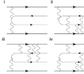
Lepton pair production in relativistic ion collision to all orders in with logarithmic accuracy is studied in [194] where the matrix elements are separated in different classes, see Fig. 5, according to numbers of photon lines attached to a given nucleus
| (133) |
The Born amplitude corresponding to the lowest order in with one photon line attached to each nucleus was computed by Landau and Lifshitz [99] who obtained the famous dependence of the cross-section in (30). It should be mentioned that the Racah formula (31) in contrast with the Landau and Lifshitz result (30) contains also terms proportional to and . These terms come from the absolute square of and and their interference with the Born amplitude [191]. Their result for the Coulomb corrections which is defined as the difference between the full cross-section and the Born approximation, in order is of the “Bethe–Maximon” type [191]
| (134) |
The Coulomb corrections here are up to -term in the Racah formula (31).
The calculations mentioned above were all made as early as in the 1930s. Clearly, at that time only pair production was discussed. However, these calculations can be considered for any lepton pair production, for example pair production, as long as the total energy in the center of mass of the system is large enough. However, simple substitution , where stands for any lepton is not sufficient since when the energy reaches the inverse radius of the nucleus the electric field of the nucleus cannot be approximated as a Coulomb field of a point-like particle [195]. The review of computation for lepton pair production can be found in [196] and [101].
Another effect of large enough collision energy is multiple pair production. Early work on this subject started with the observation that the impact-parameter-dependent total pair production probability computed in the lowest order perturbation theory is larger than one. The analysis of Ref. [190] devoted to the study of the corresponding Feynman diagrams in the high-energy limit leads to the probability of lepton pair production obeying the Poisson distribution. For a review of this topic see [189].
Two photon particle pair production by collision of two electrons or electron and positron (see Fig. 1, where 4-momenta and correspond to their momenta) were studied in storage rings in Novosibirsk ( [197]) and in Frascati at ADONE ( [198], [199], [200]), see also [201]. At high energy the total cross-section of two photon production of lepton pairs is given by [99, 101]
| (135) |
see c.f. Eq. (30).
4.7 QED description of pair production
We turn now to a Sauter-Heisenberg-Euler process in QED. An external electromagnetic field is incorporated by adding to the quantum field in (107) an unquantized external vector potential , so that the total interaction becomes
| (136) |
Instead of an operator formulation, one can derive the quantum field theory from a functional integral formulation, see e.g. [202], in which the quantum mechanical partition function is described by
| (137) |
to be integrated over all fluctuating electromagnetic and Grassmannian electron fields. The normalized quantity gives the amplitude for the vacuum to vacuum transition in the presence of the external classical electromagnetic field:
| (138) |
where is the initial vacuum state at the time , and is the final vacuum state at the time . By selecting only the one-particle irreducible Feynman diagrams in the perturbation expansion of one obtains the effective action as a functional of :
| (139) |
In general, there exists no local effective Lagrangian density whose space-time integral is . An infinite set of derivatives would be needed, i.e., would have the arguments , containing gradients of arbitrary high order. With presently available methods it is possible to calculate a few terms in such a gradient expansion, or a semi-classical approximation à là JWKB for an arbitrary but smooth space-time dependence (see Section 3.21ff in Ref. [202]). Under the assumption that the external field varies smoothly over a finite space-time region, we may define an approximately local effective Lagrangian ,
| (140) |
where is the spatial volume and time interval .
For a large time interval , the amplitude of the vacuum to vacuum transition (138) has the form,
| (141) |
where is the difference between the vacuum energies in the presence and the absence of the external field, is the vacuum decay rate, and the time over which the field is nonzero. The probability that the vacuum remains as it is in the presence of the external classical electromagnetic field is
| (142) |
This determines the decay rate of the vacuum in an external electromagnetic field:
| (143) |
The vacuum decay is caused by the production of electron and positron pairs. The external field changes the energy density by
| (144) |
4.7.1 Schwinger formula for pair production in uniform electric field
The Dirac fields appears quadratically in the partition functional (137) and can be integrated out, leading to
| (145) |
where Det denotes the functional determinant of the Dirac operator. Ignoring the fluctuations of the electromagnetic field, the result is a functional of the external vector potential :
| (146) |
The infinitesimal constant with specifies the treatment of singularities in energy integrals. From Eqs. (138)–(146), the effective action (142) is given by
| (147) |
where Tr denotes the functional and Dirac trace. In physical units, this is of order . The result may be expressed as a one-loop Feynman diagram, so that one speaks of one-loop approximation. More convenient will be the equivalent expression
| (148) |
where
| (149) |
where , . Using the identity
| (150) |
Eq. (148) becomes
| (151) |
where are the diagonal matrix elements in the local basis . This is defined by the matrix elements with the momentum eigenstates being plane waves: . The symbol denotes integral in space-time and the trace in spinor space. For constant electromagnetic fields, the integrand in (151) does not depend on , and commutes with all other operators. This will allows us to calculate the exponential in Eq. (151) explicitly. The presence of in the mass term ensures convergence of integral for .
If only a constant electric field is present, it may be assumed to point along the -axis, and one can choose a gauge such that is the only nonzero component of . Then one finds
| (152) |
where the symbol denotes the trace in spinor space. Using the commutation relation , where , one computes the exponential term in the effective action (151) (c.e.g. [89])
| (153) |
The second term in Eq. (151) is obtained by setting in Eq. (153), so that the effective action (151) yields,
| (154) |
Since the field is constant, the integral over gives a volume factor, and the effective action (151) can be attributed to the space-time integral over an effective Lagrangian (140)
| (155) |
By expanding the integrand in Eq. (155) in powers of , one obtains,
| (156) |
The small- divergence in the integrand,
| (157) |
is proportional to the electric term in the original Maxwell Lagrangian. The divergent term (157) can therefore be removed by a renormalization of the field . Thus we subtract a counterterm in Eq. (155) and form
| (158) |
Remembering Eq. (143), we find from (158) the decay rate of the vacuum per unit volume
| (159) |
The integral (159) can be evaluated analytically by the method of residues. Since the integrand is even, the integral can be extended to the entire -axis. After this, the integration contour is deformed to enclose the negative imaginary axis and to pick up the contributions of the poles of the function at . The result is
| (160) |
This result, i.e. the Schwinger formula [25, 26, 27] is valid to lowest order in for arbitrary constant electric field strength.
An analogous calculation for a charged scalar field yields
| (161) |
which generalizes the Weisskopf treatment being restricted to the leading term . These Schwinger results complete the derivation of the probability for pair productions. The leading -terms of (160) and (161) agrees with the JWKB results we discuss in Section 2.5, and thus the correct Sauter exponential factor (44) and Heisenberg-Euler imaginary part of the effective Lagrangian (102).
Narozhny and Nikishov [33] have expressed Eq. (142) through the probability of one pair production , of pair production with as well as the average number of pair productions
| (162) |
where is the probability of pair production, and the probability of one pair production is,
| (163) |
The average number of pair productions is then given by
| (164) |
which is the quantity directly related to the experimental measurements.
4.7.2 Pair production in constant electromagnetic fields
Since the QED theory is gauge and Lorentz invariant, effective action and Lagrangian are expressed as functionals of the scalar and pseudoscalar invariants (69). Thus they must be invariant under the discrete duality transformation:
| (165) |
i.e.,
| (166) |
This implies that in the case and , results can be simply obtained by replacing in Eqs. (153), (158), (159):
| (167) |
and
| (168) |
In the presence of both constant electric and magnetic fields and , we adopt parallel and pointing along the -axis in the center-of-fields frame, as discussed after Eqs. (60), (61), (62). We can choose a gauge such that only , are nonzero. Due to constant fields, the exponential in the effective action Eq. (151) can be factorized into a product of the magnetic part and the electric part. Following the same method used to compute the electric part (152,153), one can compute the magnetic part by using the commutation relation , where . Or one can make the substitution (165) to obtain the magnetic part, based on the discrete symmetry of duality. As results, Eqs. (152), (153) become
| (169) |
and
| (170) |
In this special frame, the effective Lagrangian is then given by
| (171) |
Using definitions in Eqs. (69), (70), (71), we obtain the effective Lagrangian
| (172) |
and the decay rate
| (173) |
in terms of the invariants and (71) for arbitrary electromagnetic fields and .
The integral (173) is evaluated as in Eq. (160) by the method of residues, and yields [25, 26, 27]
| (174) |
which reduces for () correctly to (160). The -term is the JWKB approximation (73).
The analogous result for bosonic fields is
| (175) |
where the first term corresponds to the Euler-Heisenberg result (102). Note that the magnetic field produces in the fermionic case an extra factor in each term which enhances the decay rate. The bosonic series (175), on the other hand, carries in each term a suppression factor . The average number (164) is given by
| (176) |
The decay rate gives the number of electron–positron pairs produced per unit volume and time. The prefactor can be estimated on dimensional grounds. It has the dimension of , i.e., . This arises from the energy of a pair divided by the volume whose diameter is the Compton wavelength , produced within a Compton time . The exponential factor suppresses pair production as long as the electric field is much smaller than the critical electric field , in which case the JWKB results (73) and (74) are good approximations.
The general results (174),(175) was first obtained by Schwinger [25, 26, 27] for scalar and spinor electrodynamics (see also Nikishov [28], Batalin and Fradkin [29]). The method was extended to special space-time-dependent fields in Refs. [30, 31, 32, 33, 34]. The monographs [89, 145, 203, 204, 205] can be consulted about more detailed calculation, discussion and bibliography.
4.7.3 Effective nonlinear Lagrangian for arbitrary constant electromagnetic field
Starting from the integral form of Heisenberg and Euler Lagrangian (172) we find explicitly real and imaginary parts of the effective Lagrangian (172) for arbitrary constant electromagnetic fields and [35]. The essential step is to reach a direct analytic form resulting from performing the integration. We use the expressions [206],
| (177) | ||||
| (178) |
and obtain for the finite effective Lagrangian of Heisenberg and Euler integral representation,
| (179) |
where divergent terms , and are excluded from the sum, as indicated by a prime. The symbol denotes the complimentary Kronecker- which vanishes for . The divergent term with is eliminated by the zero-field subtraction in Eq. (172), while the divergent terms and
| (180) |
are eliminated by the second subtraction in Eq. (172). This can be seen by performing the sums
| (181) |
where is the Riemann function.
The infinitesimal accompanying the mass term in the -integral (179) is equivalent to replacing by . This implies that is to be integrated slightly below (above) the real axis for (). Equivalently one may shift the () variables slightly upwards (downwards) to () in the complex plane.
In order to calculate the finite effective Lagrangian (179), the factor is divided into its sin and cos parts:
| (182) | ||||
| (183) |
The sin part (182) has an even integrand allowing for an extension of the -integral over the entire -axis. The contours of integration can then be closed by infinite semicircles in the half plane, the integration receives contributions from poles , so that the residue theorem leads to,
| (184) | ||||
| (185) |
The first part (184) leads to the exact non-perturbative Schwinger rate (174) for pair production.
The second term, as we see below, is canceled by the imaginary part of the cos term. In fact, shifting , we rewrite the cos part of effective Lagrangian (183) as
| (186) |
In the first term of magnetic part, singularities and appear in integrating -axis. We decompose
| (187) |
where indicates the principle value under the integral. The integrals over the -functions give
| (188) |
which exactly cancels the second part (185) of the sin part .
It remains to find the principle-value integrals in Eq. (186), which corresponds to the real part of the effective Lagrangian
| (189) |
We rewrite the cos function as and make the rotations of integration contours by respectively,
| (190) | |||||
Using the formulas (see Secs. 3.354, 8.211.1 and 8.211.2 in Ref. [206])
| (191) |
where is the exponential-integral function,
| (192) |
we obtain the principal-value integrals (190),
| (193) |
Having so obtained the real part of an effective Lagrangian for an arbitrary constant electromagnetic field we recover the usual approximate results by suitable expansion of the exact formula. With the help of the series and asymptotic representation (see formula 8.215 in Ref. [206]) of the exponential-integral function for large , corresponding to weak electromagnetic fields (),
| (194) |
and Eq. (193), we find,
| (195) |
Applying the summation formulas (181), the weak field expansion (195) is seen to agree with the Heisenberg and Euler effective Lagrangian [7],
| (196) |
which is expressed in terms of a powers series of weak electromagnetic fields up to . The expansion coefficients of the terms of order have the general form . As long as the fields are much smaller than , the expansion converges.
On the other hand, we can address the limiting form of the effective Lagrangian (193) corresponding to electromagnetic fields (). We use the series and asymptotic representation (formulas 8.214.1 and 8.214.2 in Ref. [206]) of the exponential-integral function for small ,
| (197) |
with being the Euler-Mascheroni constant, we obtain the leading terms in the strong field expansion of Eq. (193),
| (198) |
In the case of vanishing magnetic field and in Eq. (198), we have,
| (199) |
for a strong electric field . In the case of vanishing electric field and in Eq. (198), we obtain for the strong magnetic field ,
| (200) |
The () term is the one obtained by Weisskopf [24].
We have presented in Eqs. (184), (185), (188), (193) closed form results for the one-loop effective Lagrangian (172) for arbitrary strength of constant electromagnetic fields. The results will receive fluctuation corrections from higher loop diagrams. These carry one or more factors , , … and are thus suppressed by factors . Thus results are valid for all field strengths with an error no larger than roughly 1%. If we include, for example, the two-loop correction, the first term in the Heisenberg and Euler effective Lagrangian (196) becomes [145]
| (201) |
Readers can consult the recent review article [207], where one finds discussions and computations of the effective Lagrangian at the two-loop level, and [208] for discussion of pair production rate.
4.8 Theory of pair production in an alternating field
When the external electromagnetic field is space-time-dependent, i.e., the exponential in Eq. (151) can no longer be calculated exactly. In this case, JWKB methods have to be used to calculate pair production rates [36, 30, 31, 32, 37, 209, 210, 30, 31, 32]. The aim of this section is to show how one can use a semi-classical JWKB approach to estimate the rate of pair production in an oscillating electric field as first indicated by Brezin and Itzykson in Ref. [36]. They evaluated the production rate of charged boson pairs. The results they obtained can be straightforwardly generalized to charged fermion case, since the spins of charged particles contribute essentially with a counting factor to the final results (see Secs. 2.5 and 4.7.1). Thus, let the electromagnetic potential be directed, uniform in space and periodic in time with frequency :
| (202) |
Then the electric field is directed, uniform in space and periodic in time as well. The electric field strength is given by . It is assumed that the electric field is adiabatically switched on and damped off in a time , which is much larger than the period of oscillation . Suppose also that is much larger than the Compton time of the created particle , i.e.,
| (203) |
where , being the 3-momentum of the created particle. Furthermore, is assumed to be much smaller than , i.e., (see Eq. (59)).
We have to study the time evolution of a scattered wave function representing the production of particle and antiparticle pairs in the electromagnetic potential (202). As usual, an antiparticle can be thought of as a wave-packet moving backward in time. Therefore, for large positive time (forward) only positive energy modes () contribute to . Similarly, for large negative times both positive energy and negative energy modes () contribute to which satisfies the differential equation [36]:
| (204) |
where the “variable frequency” is defined as
| (205) |
The JWKB method suggests a general solution of the from
| (206) |
where the boundary conditions at large positive and negative times are:
| (207) |
The backward scattering amplitude for large negative time () represents the probability of antiparticle production.
The normalization condition implies
| (208) |
Eq. (204) can be written in terms of the scattering amplitudes as
| (209) |
or, which is the same,
| (210) | |||||
| (211) |
It follows from assumption (203) that vanishes as , i.e.,
| (212) |
More precisely
| (213) |
Therefore, and slowly vary in time and tend to constants as . The phase oscillates very rapidly as compared to the variation of and , for . In the zeroth order the oscillating terms in Eqs. (210), (211) are negligible and one finds
| (214) |
which duly satisfy the boundary conditions, and
| (215) |
where (203) and (213) have been used. gives information about the probability of particle-antiparticle pair production. Namely, the probability of pair production per unit volume and time is given by
| (216) | |||||
Since is a periodic function with the same frequency as one can make a Fourier series expansion:
| (217) |
Defined a renormalized frequency via one finds
| (218) |
so that
| (219) |
Consequently, the probability of pair production (216) is,
| (220) |
where and are determined via Eq. (217) as
| (221) |
The expression for contains a very rapidly oscillating phase factor with frequency of the order of , and it decreases very rapidly in terms of imaginary time . Its evaluation requires the application of the steepest-descent method in the complex time plane. This is done by selecting a proper contour turning in a neighborhood of the saddle point and following the steepest-descent line, so as to find the main contributions to the integral in Eq. (221). The saddle point originates from branch points and poles in Eq. (221), which are the zeros of . Mathematical details can be found in Ref. [36]. One finds
| (222) |
where
| (223) |
and the saddle point is .
The exponential factor in Eq. (222) indicates that particle-antiparticle pairs tend to be emitted with small momenta. This allows one to estimate the right-hand side of Eq. (222) as follow: (i) is set equal to zero, moreover, the range of the -integration is of the order of as suggested by the classical equation of motion (204); (ii) is replaced by its average value . As a result, one obtains [36],
| (224) |
where , and
| (225) |
where is the Gauss hypergeometrical function. The function is monotonically increasing:
| (226) |
which indicates that the integral in (224) is strongly dominated by values in a neighborhood of . This allows one to approximately perform the integration and leads to the rate of pair production of charged bosons [36],
| (227) |
Analogously, the rate of pair production of charged fermions can be approximately obtained from Eq. (227) by taking into account two helicity states of fermions (see Secs. 2.5 and 4.7.1),
| (228) |
This formula has played an important role in recent studies of electron and positron pair production by laser beams, which we will discuss in some details in Section 6.2. Momentum spectrum of electrons and positrons, produced from the vacuum, was calculated in [30, 31, 37, 32]. For this distribution is concentrated along the direction of electric field, while for it approaches isotropic one.
Unfortunately, it appears very difficult to produce a macroscopic electric field with strength of the order of the critical value (1) and lifetime long enough () in any ground laboratory to directly observe the Sauter-Euler-Heisenberg-Schwinger process of electron–positron pair production in vacuum. The same argument applies for the production of any other pair of fermions or bosons. In the following Section, we discuss some ideas to experimentally create a transient electric field in Earth-bound laboratories, whose lifetime is expected to be long enough (larger than ) for the pair production process to take place.
4.9 Nonlinear Compton scattering and Breit-Wheeler process
In Section 2.2, we have discussed the Breit–Wheeler process [2] in which an electron–positron pair is produced in the collision of two real photons (3). The cross-section they obtained is , where is the classical electron radius, see Eq. (24). This lowest order photon-photon pair production cross-section is so small that it is difficult to observe creation of pairs in the collision of two high-energy photon beams, even if their center of mass energy is larger than the energy-threshold MeV.
In the previous Sections we have seen that in strong electromagnetic fields in lasers the effective nonlinear terms (196) become significant and therefore, the interaction needs not to be limited to initial states of two photons [61, 62]. A collective state of many interacting laser photons occurs.
We turn now to two important processes [38, 39] emerging in the interaction of an ultrarelativistic electron beam with a terawatt laser pulse, performed at SLAC [63], when strong electromagnetic fields are involved. The first process is the nonlinear Compton scattering, in which an ultrarelativistic electron absorbs multiple photons from the laser field, but emits only a single photon via the process
| (229) |
where represents photons from the strong electromagnetic wave of the laser beam (its frequency being ), indicates the number of absorbed photons and represents a high-energy emitted photon (see Eq. (230) for cross symmetry). The theory of this nonlinear Compton effect (229) is given in Section 4.10. The same process (229) has been expressed by Bamber et al. [211] in a semi-classical framework. The second is the nonlinear Breit–Wheeler process
| (230) |
between this very high-energy photon and multiple laser photons: the high-energy photon , created in the first process, propagates through the laser field and interacts with laser photons to produce an electron–positron pair [39].
In the electric field of an intense laser beam, an electron oscillates with the frequency of the laser and its maximum velocity in unit of the speed of light is given by
| (231) |
In the case of weak electric field, and the nonrelativistic electron emits the dipole radiation well described in linear and perturbative QED. On the other hand, in the case of strong electric fields, and the ultrarelativistically oscillating electron emits multi-pole radiation. The radiated power is then a nonlinear function of the intensity of the incident laser beam. Using the maximum velocity of oscillating electrons in the electric field of laser beam, one can characterize the effect of nonlinear Compton scattering by the dimensionless parameter
| (232) |
where the subscript ‘rms’ means root-mean-square, with respect to the number of interacting laser photons with scattered electron. The parameter can be expressed as a Lorentz invariant,
| (233) |
where is the gauge potential of laser wave, and the time-average is taken over one period of laser wave, and
| (234) |
Eq. (233) shows that is the intensity parameter of laser fields, and in (232) coincides with the parameter introduced in Eq. (224) for the pair production in an alternating electric field (see Section 4.8).
4.10 Quantum description of nonlinear Compton effect
In Refs. [61, 62, 40, 41, 42, 43, 44, 45, 212, 213, 214, 215, 216, 90], the quantum theory of the interaction of free electrons with the field of a strong electromagnetic wave has been studied. The application of quantum perturbation theory to such interaction requires not only that the interaction constant should be small but also that field should be sufficiently weak. The characteristic quantity in this respect is the dimensionless invariant ratio , see (233). The photon emission processes occurring in the interaction of an electron with the field of a strong electromagnetic wave have been discussed in Ref. [90] for any value. The method used is based on an exact treatment of this interaction, while the interaction of the electron with the newly emitted photons regarded as a perturbation.
Laser beam is considered as a monochromatic plane wave, described by the gauge potential and , where wave vector (see Eq. (6)). The Dirac equation can be exactly solved [217] for an electron moving in this field of electromagnetic plane wave of an arbitrary polarization and the normalized wave function of the electron with momentum is given by (c.e.g. [90]),
| (235) | |||||
| (236) |
where is the solution of free Dirac equation and the time-average value of 4-vector,
| (237) |
is the kinetic momentum operator in the electron state (235) and the “effective mass” of the electron in the field is
| (238) |
where is given by (233). The electron becomes “heavy” in an oscillating electromagnetic field.
The -matrix element for a transition of the electron from the state to the state , with emission of a photon having momentum and polarization is given by (c.e.g. [90])
| (239) | |||||
| (240) |
where the integrand in Eq. (239) is expanded in Fourier series and expansion coefficients are in terms of Bessel functions , the scattering amplitude in Eq. (240) is obtained333The explicit expression is not given here for its complexity, see for example [90]. by integrating over . Eq. (240) shows that is an infinite sum of terms, each corresponds to an energy-momentum conservation law , indicating an electron () absorbs -photons () and emits another photon () of frequency
| (241) |
in the frame of reference where the electron is at rest (), and is the angle between and . Given the th term of the -matrix (240), the differential probability per unit volume and unit time yields,
| (242) |
Integrating over the phase space of final states , one obtains the total probability of emission from unit volume in unit time (circular polarization),
| (243) |
where , and Bessel functions ,
| (244) |
for any value. A systematic investigation of various quantum processes in the field of a strong electromagnetic wave can be found in [40, 41, 42, 43, 44, 45], in particular photon emission and pair production in the field of a plane wave with various polarizations are discussed.
We now turn to the Breit–Wheeler process for multi-photons (230). In this process, the pair production is attributed to the interaction of a high-energy photon with many laser photons in the electromagnetic laser wave. Actually, the Breit–Wheeler process for multi-photons, see Eq. (230), is related to the nonlinear Compton scattering process, see Eq. (229), by crossing symmetry. By replacement and and reverse the common sign of the expression in Eq. (240), one obtains the probability of pair production (230) by a photon (momentum ) colliding with laser photons (momentum ) per unit volume in unit time (circular polarization) [40, 41, 42, 43, 44, 45],
| (245) | |||||
where , , and Bessel functions ,
In Eq. (245), the number of laser photons must be larger than (), which is the energy threshold for the process (230) of pair production to occur.
5 Semi-classical description of pair production in a general electric field
As shown in previous sections, the rate of pair production may be split into an exponential and a pre-exponential factor. The exponent is determined by the classical trajectory of the tunneling particle in imaginary time which has the smallest action. It plays the same role as the activation energy in a Boltzmann factor with a “temperature” . The pre-exponential factor is determined by the quantum fluctuations of the path around that trajectory. At the semi-classical level, the latter is obtained from the functional determinant of the quadratic fluctuations. It can be calculated in closed form only for a few classical paths [202]. An efficient technique for doing this is based on the JWKB wave functions, another on solving the Heisenberg equations of motion for the position operator in the external field [202].
Given the difficulties in calculating the pre-exponential factor, only a few nonuniform electric fields in space or in time have led to analytic results for the pair production rate: (i) the electric field in the -direction is confined in the space , i.e., where [218, 219]; (ii) the electric field in the -direction depends only on the light-cone coordinate , i.e., [220, 221]. If the nonuniform field has the form , which will be referred as a Sauter field, the rate was calculated by solving the Dirac equation [33] in the same way as Heisenberg and Euler did for the constant electric field. For general space and time dependencies, only the exponential factor can be written down easily — the fluctuation factor is usually hard to calculate [65]. In the Coulomb field of heavy nucleus whose size is finite and charge is supercritical, the problem becomes even more difficult for bound states being involved in pair production, and a lot of effort has been spent on this issue [65, 203, 222].
If the electric field has only a time dependence , both exponential and pre-exponential factors were approximately computed by Brezin and Itzykson using JWKB methods for the purely periodic field [36]. The result was generalized by Popov in Ref. [209, 223] to more general time-dependent fields . After this, several time-independent but space-dependent fields were treated, for instance an electric field between two conducting plates [224], and an electric field around a Reissner–Nordström black hole [46].
The semi-classical expansion was carried beyond the JWKB approximation by calculating higher order corrections in powers of in Refs. [51, 52] and [53]. Unfortunately, these terms do not comprise all corrections of the same orders as explained in [54].
An alternative approach to the same problems was recently proposed by using the worldline formalism [47], sometimes called the “string-inspired formalism”. This formalism is closely related to Schwinger’s quantum field theoretic treatment of the tunneling problem, where the evaluation of a fluctuation determinant is required involving the fields of the particle pairs created from the vacuum. The worldline approach is a special technique for calculating precisely this functional determinant. Within the worldline formalism, Dunne and Schubert [48] calculated the exponential factor and Dunne et al. [49] gave the associated prefactor for various field configurations: for instance a spatially uniform, and single-pulse field with a temporal Sauter shape . For general -dependencies, a numerical calculation scheme was proposed in Ref. [225, 226, 227, 228] and applied further in [229]. For a multidimensional extension of the techniques see Ref. [50].
In this Section, a general expression is derived for the pair production rate in nonuniform electric fields pointing in the -direction recently derived in [230, 54]. A simple variable change in all formulas leads to results for electric fields depending also on time rather than space. As examples, three cases will be treated: (i) a nonzero electric field confined to a region of size , i.e., (Sauter field see Eq. (297)); (ii) a nonzero electric field in a half space, i.e., (see Eq. (318)); (iii) an electric field increasing linearly like . In addition, the process of negative energy electrons tunneling into the bound states of an electric potential with the emission of positrons will be studied, by considering the case: the electric field of harmonic potential .
5.1 Semi-classical description of pair production
The phenomenon of pair production in an external electric field can be understood as a quantum mechanical tunneling process of Dirac electrons [80, 1]. In the original Dirac picture, the electric field bends the positive and negative energy levels of the Hamiltonian, leading to a level crossing and a tunneling of the electrons in the negative energy band to the positive energy band. Let the field vector point in the -direction. In the one-dimensional potential energy (39) the classical positive and negative energy spectra are
| (246) |
where is the momentum in the -direction, the momentum orthogonal to it, and . For a given energy , the tunneling takes place from to determined by in Eq. (246)
| (247) |
The points are the turning points of the classical trajectories crossing from the positive energy band to the negative one at energy . They satisfy the equations
| (248) |
This energy level crossing is shown in Fig. 6 for the Sauter potential .
5.1.1 JWKB transmission probability for Klein–Gordon Field
The probability of quantum tunneling in the -direction is most easily studied for a scalar field which satisfies the Klein–Gordon equation (38). If there is only an electric field in the -direction which varies only along , a vector potential with the only nonzero component (39) is chosen, and the ansatz , is made with a fixed momentum in the -direction and an energy , and Eq. (38) becomes simply
| (249) |
By expressing the wave function as an exponential
| (250) |
where is some normalization constant, the wave equation becomes a Riccati equation for :
| (251) |
where the function is the solution of the equation
| (252) |
The solution of Eq. (251) can be found iteratively as an expansion in powers of :
| (253) |
Neglecting the expansion terms after leads to the JWKB approximation for the wave functions of positive and negative energies (see e.g. [88, 202])
| (254) |
where is the eikonal
| (255) |
Between the turning points , whose positions are illustrated in Fig. 6, the momentum is imaginary and it is useful to define the positive function
| (256) |
The tunneling wave function in this regime is the linear combination
| (257) |
Outside the turning points, i.e., for and , there exist negative energy and positive energy solutions for and for positive . On the left-hand side of , the general solution is a linear combination of an incoming wave running to the right and outgoing wave running to the left:
| (258) |
On the right-hand of , there is only an outgoing wave
| (259) |
The connection equations can be solved by
| (260) |
The incident flux density is
| (261) |
which can be written as
| (262) |
where is the velocity and the density of the incoming particles. Note that the -dependence of and cancel each other. By analogy, the outgoing flux density is .
5.1.2 Rate of pair production
From the considerations given above, the transmission probability
| (263) |
is found to be the simple exponential
| (264) |
In order to derive from (263) the total rate of pair production in the electric field, it must be multiplied with the incident particle flux density at the entrance of the tunnel. The particle velocity at that point is , where the relation between and is given by Eq. (248):
| (265) |
This must be multiplied with the particle density which is given by the phase space density . The incident flux density at the tunnel entrance is therefore
| (266) |
and the extra factor is equal to for electrons with two spin orientations444By setting equal to one can obtain the tunneling result also for spin- particles although the Dirac picture is no longer applicable..
It is useful to change the variable of integration from to defined by
| (267) |
and to introduce the notation for the electric field , where is the inverse function of (267), the equations in (248) reduce to
| (268) |
In terms of the variable , the JWKB transmission probability (264) can be rewritten as
| (269) |
Here a standard field strength has been introduced to make the integral in the exponent dimensionless, which is abbreviated by
| (270) |
The first term in the exponent of (269) is equal to .
At the semi-classical level, tunneling takes place only if the potential height is larger than and for energies for which there are two real turning points . The total tunneling rate is obtained by integrating over all incoming momenta and the total area of the incoming flux. The JWKB-rate per area is
| (271) |
Using the relation following from (265)
| (272) |
the alternative expression is obtained
| (273) |
where is obtained by solving the differential equation (272).
The integral over cannot be done exactly. At the semi-classical level, this is fortunately not necessary. Since is proportional to , the exponential in (269) restricts the transverse momentum to be small of the order of , so that the integral in (273) may be calculated from an expansion of up to the order :
| (274) | |||||
where , and
| (275) | |||||
The integral over in (273) is approximately performed as follows:
| (276) | |||
where
| (277) |
The electric fields at the tunnel entrance in the prefactor of (273) can be expanded similarly to first order in . If denotes the solutions of (265) at , it is found that for small :
| (278) |
so that
| (279) |
Here the extra term proportional to can be neglected in the semi-classical limit since it gives a contribution to the prefactor of the order . Thus the JWKB-rate (273) of pair production per unit area is obtained
| (280) |
where is short for . At this point it is useful to return from the integral introduced in (273) to the original energy integral in (271), so that the final result is
| (281) |
where -integration is over all crossing energy levels.
These formula can be approximately applied to the three-dimensional case of electric fields and potentials at the points where the tunneling length (52) is much smaller than the variation lengths of electric potentials in the -plane,
| (282) |
At these points , one can arrange the tunneling path and momentum in the direction of electric field, corresponding perpendicular area for incident flux and perpendicular momentum . It is then approximately reduced to a one-dimensional problem in the region of size around these points. The surfaces and associated with the classical turning points are determined by Eqs. (267) and Eqs. (268) for a given energy . The JWKB-rate of pair production (280) can then be expressed as a volume integral over the rate density per volume element
| (283) |
On the right-hand side it is useful to rewrite the rate as the time derivative of the number of pair creation events , so that one obtains an event density in four-space
| (284) |
Here and are related by the function which is obtained by solving (272).
It is now useful to observe that the left-hand side of (284) is a Lorentz invariant quantity. In addition, it is symmetric under the exchange of time and , and this symmetry will be exploited in the next section to relate pair production processes in a -dependent electric field to those in a time-dependent field .
5.1.3 Including a smoothly varying -field parallel to
The results presented above can easily be extended for the presence of a constant magnetic field parallel to . Then the wave function factorizes into a Landau state and a spinor function first calculated by Sauter [20]. In the JWKB approximation, the energy spectrum is still given by Eq. (246), but the squared transverse momenta is quantized and must be replaced by discrete values corresponding to the Landau energy levels. From the known nonrelativistic levels for the Hamiltonian one extracts immediately the replacements (63). Apart from the replacement (63), the JWKB calculations remain the same. Thus one must only replace the integration over the transverse momenta in Eq. (276) by the sum over all Landau levels with the degeneracy . Thus, the right-hand side becomes
| (285) |
where and are as in (63). The result is, for spin-0 and spin-1/2:
| (286) |
where
| (287) |
The result remains approximately valid if the magnetic field has a smooth -dependence varying little over a Compton wavelength .
In the following only nonuniform electric fields without a magnetic field are considered.
5.2 Time-dependent electric fields
The semi-classical considerations given above can be applied with little change to the different physical situation in which the electric field along the -direction depends only on time rather than . Instead of the time itself it is better to work with the zeroth length coordinate , as usual in relativistic calculations. As an intermediate step consider for a vector potential
| (288) |
with the electric field
| (289) |
The associated Klein–Gordon equation (38) reads
| (290) |
The previous discussion was valid under the assumption , in which case the ansatz
led to the field equation (249). For the present discussion it is useful to write the ansatz as with , and Eq. (249) in the form
| (291) |
Now assume that the electric field depends only on . Then the ansatz leads to the field equation
| (292) |
5.3 Applications
Now formulas (281) or (280) are applied to various external field configurations capable of producing electron–positron pairs.
5.3.1 Step-like electric field
First one checks the result for the original case of a constant electric field where the potential energy is the linear function . Here the function (270) becomes trivial
| (294) |
which is independent of (or ). The JWKB-rate for pair production per unit time and volume is found from Eq. (280) to be
| (295) |
where . This expression contains the exponential found by Sauter [20], and the correct prefactor as calculated by Heisenberg and Euler [7], and by Schwinger [25, 26, 27].
5.3.2 Sauter electric field
Let us now consider the nontrivial Sauter electric field localized within finite slab in the -plane with the width in the -direction. A field of this type can be produced, e.g., between two opposite charged conducting plates. The electric field in the -direction and the associated potential energy are given by
| (297) |
where
| (298) |
From now on natural units, in which energies are measured in units of , are used. Figure 6 shows the positive and negative energy spectra of Eq. (246) for in particular the energy gap and energy level crossings. From Eq. (248) one finds the classical turning points
| (299) |
Tunneling is possible for all energies satisfying
| (300) |
for the strength parameter .
One may invert Eq. (267) to find the relation between and :
| (301) |
In terms of the function , the Eq. (299) reads simply .
Inserting (301) into the equation for in Eq. (297), one obtains
| (302) |
and of Eqs. (270), (274) and (275) are calculated:
| (303) |
and
| (304) |
Substituting the functions and into Eqs. (280) and (281), one obtains the general expression for the pair production rate per volume slice at a given tunnel entrance point or the associated energy . The pair production rate per area is obtained by integrating over all slices permitted by the energy inequality (300).
In Fig. 7, the slice dependence of the integrand in the tunneling rate (280) for the Sauter potential (297) is shown and compared with the constant field expression (295) of Euler and Heisenberg, if it is evaluated at the -dependent electric field . This is done once as a function of the tunnel entrance point and once as a function of the associated energy . On each plot, the difference between the two curves illustrates the nonlocality of the tunneling process555Note that omitting the -integral in the rate formula (280) does not justify calling the result a “local production rate”, as done in the abstract of Ref. [229]. The result is always nonlocal and depends on all gradients of the electric field..
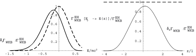
The integral is dominated by the region around , where the tunneling length is shortest [see Fig. 6] and tunneling probability is largest. Both functions and have a symmetric peak at . Around the peak they can be expanded in powers of as
| (305) | |||||
and
| (306) | |||||
The exponential has a Gaussian peak around whose width is of the order of . This implies that in the semi-classical limit, one may perform only a Gaussian integral and neglect the -dependence of the prefactor in (281). Recalling that in this section is in natural units with , one should replace by and can perform the integral over approximately as follows
| (307) | |||||
For convenience, the limits of integration over is extended from the interval to . This introduces exponentially small errors and can be ignored.
Using the relation (298) one may replace by , and obtain
| (308) |
This approximate result agrees 666See Eq. (63) of Dunne and Schubert [48], and replace there . It agrees also with the later paper by Dunne et al. [49] apart from a factor 2. with that obtained before with a different, somewhat more complicated technique proposed by Dunne and Schubert [48] after the fluctuation determinant was calculated exactly in [49] with the help of the Gelfand–Yaglom method, see Section 2.2 in Ref. [202]. The advantage of knowing the exact fluctuation determinant could not, however, be fully exploited since the remaining integral was calculated only in the saddle point approximation. The rate (308) agrees with the leading term of the expansion (42) of Kim and Page [53]. Note that the higher expansion terms calculated by the latter authors do not yet lead to proper higher order results since they are only of type II and III in the list after Eq. (284). The terms of equal order in in the expansion (253) of the solution of the Riccati equation are still missing.
Using the transformation rules (293), it is straightforward to obtain the pair production rate of the Sauter type of electric field depending on time rather than space. According to the transformation rules (293), one has to replace , where is the characteristic time over which the electric field acts—the analog of in (297). Thus the field (297) becomes
| (309) |
According to the same rules, one must also replace , where
| (310) |
This brings of Eq. (303) to the form
| (311) |
and yields the pair production rate
| (312) |
where is the number of pairs produced per unit thickness in a spatial shell parallel to the -plane. This is in agreement with Ref. [49].
Note also that the constant field result (295) of Euler and Heisenberg cannot be deduced from (308) by simply taking the limit as one might have expected. The reason is that the saddle point approximation (307) to the integral (281) becomes invalid in this limit. Indeed, if is large in Eqs. (303) and (304), these become
| (313) |
and the integral in (281) becomes approximately
| (314) |
For not too large , the integral can be evaluated in the leading Gaussian approximation
| (315) |
corresponding to the previous result (308) for large-. For a constant field, however, where the integrands becomes flat, the Gaussian approximation is no longer applicable. Instead one must first set in the integrand of (314), making it constant. Then the integral (314) becomes777This treatment is analogous to that of the translational degree of freedom in instanton calculations in Section 17.3.1 of [202] [see in particular Eq. (17.112)].
| (316) |
Inserting this into (281) one recovers the constant field result (295). One must replace by to comply with the relation (272) from which one obtains
In order to see the boundary effect on the pair production rate, this section is closed with a comparison between pair production rates in the constant field (295) and Sauter field (308) for the same field strength in the volume . The ratio of pair production rates (308) and (295) in the volume is defined as
| (317) |
The soft boundary of the Sauter field (297) reduces its pair production rate with respect to the pair production rate (295) computed in a constant field of width . The reduction is shown quantitatively in Fig. 8, where curves are plotted for the rates (295) and (308), and and for their ratio (317) at and [recall (298)]. One can see that the reduction is significant if the width of the field slab shrinks to the size of a Compton wavelength .
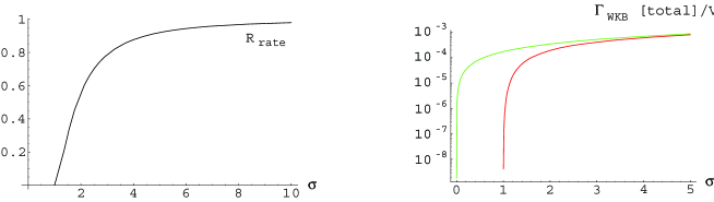
5.3.3 Constant electric field in half space
As a second application consider an electric field which is zero for and goes to over a distance as follows:
| (318) |
where . In Fig. 9, the positive and negative energy spectra defined by Eq. (246) for are plotted to show energy gap and level crossing.
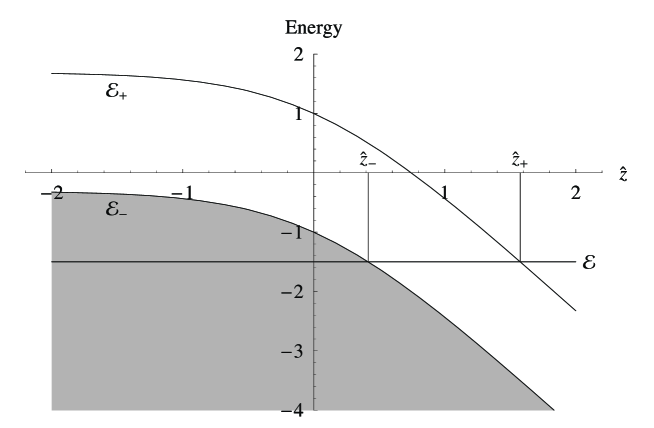
From Eq. (248) one finds now the classical turning points [instead of (299)]
| (319) |
For tunneling to take place, the energy has to satisfy
| (320) |
and must be larger than . Expressing in terms of as
| (321) |
so that , one finds the electric field in the form
| (322) |
Inserting this into Eq. (270) and expanding in powers one obtains
| (323) | |||||
where is a modified Bessel function. Expanding in powers of :
| (324) |
one can identify
| (325) | |||||
| (326) |
The integral over in Eq. (281) starts at where the integrand rises from 0 to as exceeds a few units of . The derivative of drops from to over this interval. Hence the derivative is peaked around some value . Thus the integral is performed by parts as
| (327) |
The first term can be rewritten with the help of as , thus giving rise to the decay rate (295) in the volume , and the second term gives only a small correction to this. The second term in Eq. (327) shows that the boundary effects reduce the pair production rate compared with the pair production rate (295) in the constant field without any boundary.
5.4 Tunneling into bound States
We turn now to the case in which instead of an outgoing wave as given by (259) there is a bound state. A linearly rising electric field whose potential is harmonic is considered:
| (328) |
It will be convenient to parametrize the field strength in terms of a dimensionless reduced electric field as . In Fig. 10, the positive and negative energy spectra defined by Eq. (246) for are plotted to show energy gap and level crossing for (left) and (right).
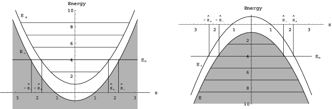
If is positive, Eq. (248) yields for ,
| (329) |
and mirror-reflected turning points for , obtained by exchanging in (329). Negative energy electrons tunnel into the potential well , where , forming bound states. The associated positrons run off to infinity.
5.4.1 JWKB transmission probability
Due to the physical application to be discussed in the next section, here only the tunneling process for on the left-hand side of Fig. 10 will be studied. One can consider the regime with the turning pints . The incident wave and flux for pointing in the positive -direction are given by Eqs. (258) and (261). The wave function for has the form Eq. (257) with the replacement . The transmitted wave is now no longer freely propagating as in (259), but describes a bound state of a positive energy electron:
| (330) |
The Sommerfeld quantization condition
| (331) |
fixes the energies . The connection rules for the wave functions (257) and (330) at the turning point determine
| (332) |
Assuming the states to be initially unoccupied, the transmitted flux to these states at the classical turning point is
| (333) |
From Eqs. (261), (333), and (263) one then finds the JWKB transmission probability for positrons to fill these bound states leaving a positron outside:
| (334) |
which has the same form as Eq. (56). The same result is obtained once more for with turning points , which can be obtained from (334) by the mirror reflection .
5.4.2 Energy spectrum of bound states
From Eq. (252) for and Eq. (328) for the potential , the eikonal (331) is calculated to determine the energy spectrum of bound states
| (335) | |||||
where , are complete elliptical integrals of the first and second kind, respectively, and . The Sommerfeld quantization rule (331) becomes
| (336) | |||
For any given transverse momentum , this determines the discrete energies .
5.4.3 Rate of pair production
By analogy with Eqs. (271) and (281), the transmission probability (334) must now be integrated over all incident particles with the flux (266) to yield the rate of pair production:
| (337) | |||||
| (338) |
In obtaining these expressions one has used the energy conservation law to perform the integral over . This receives only contributions for where . The factor accounts for the equal contributions from the two regimes and . The previous relation (272) is now replaced by
| (339) |
Using Eq. (267) and expressing in terms of as
| (340) |
one calculates , and find the electric field in the form
| (341) |
Inserting this into Eq. (270) one obtains
| (342) | |||||
where and . Expanding in powers of one finds the zeroth order term
| (343) |
and the derivative
| (344) | |||||
where .
6 Phenomenology of electron–positron pair creation and annihilation
6.1 annihilation experiments in particle physics
The process predicted by Dirac was almost immediately observed [3]. The annihilation experiments have since became possibly the most prolific field of research in the active domain of particle physics. The Dirac pair annihilation process (2) has no energy threshold and the energy release in the collision is larger than . This process is the only one in the limit of low energy. As the energy increases the collision produces not only photons through the Dirac process (230) but also other particles. For early work in this direction, predicting resonances for pions, K-mesons etc., see [231]. Production of such particles are achievable and precisely conceived in experimental particle physics, but hardly possible with the vacuum polarization process . In particular when the energy in the center of mass is larger than twice muon mass about 100 times electron mass, the electron and positron electromagnetically annihilate into two muons via the intermediation of a virtual photon. The cross-section in the center of mass frame is given by [232]
| (345) |
where is the muon part of the vacuum polarization tensor and the square of energy of the center of mass frame, where are 4-momenta of positron and electron. At very high energy , .
At very high energies of the order of several GeV, electron and positron electromagnetically annihilate into hadrons, whose cross-section has the same structure as the cross-section (345) with replaced by the hadron part of the vacuum polarization tensor ,
| (346) |
The two cross-sections (345) and (346) are comparable, of the order of a few tens of nanobarns (cm2). It is traditional to call the ratio of hadronic to electromagnetic annihilation cross-sections [232],
| (347) |
As the energy of electron and positron collision increases and reaches the mass–energy thresholds of constituents of hadrons, i.e. “quarks”, narrow resonances occurs, see Fig. 11 for the ratio as a function of measured at SLAC [233]. These resonances correspond to production of particles such as , etc.

This provides a fruitful investigation of hadron physics. For a review of this topic see [101].
As the center of mass energy reaches the electroweak scale (several hundred GeVs), electron and positron annihilation process probes a rich domain of investigating electroweak physics, see for instance Refs. [234, 235]. Recent experiments on collisions at LEP, SLAC and the Tevatron allowed precision tests of the electroweak Standard Model. In [236, 237] the results of these precision tests together with implications on parameters, in particular Higgs boson mass, as well as constraints for possible new physics effects are discussed.
Electron and positron collisions are used to produce many particles in the laboratory, which live too short to occur naturally. Several electron–positron colliders have been built and proposed for this purpose all over the world (CERN, SLAC, INP, DESY, KEK and IHEP), since the first electron–positron collider the “Anello d’Accumulazione” (AdA) was built by the theoretical proposal of Bruno Touschek in Frascati (Rome) in 1960 [55]. Following the success of AdA (luminosity /(cm2 sec), beam energy 0.25GeV), it was decided to build in the Frascati National Laboratory a storage ring of the same kind, Adone and then Daphne (luminosity /(cm2sec), beam energy 0.51GeV), with the aim of exploring the new energy range in subnuclear physics opened by the possibility of observing particle-antiparticle interactions with center of mass at rest. The biggest of all is CERN’s Large Electron Positron (LEP) collider [148], which began operation in the summer of 1989 and have reached a maximal collision energy of 206.5 GeV. The detectors around the LEP ring have been able to perform precise experiments, testing and extending our knowledge of particles and their strong, electromagnetic and weak interactions, as described by the Standard Model for elementary particle physics.
All these clearly show how the study of reaction introduced by Dirac have grown to be one of the most prolific field in particle physics and have received remarkable verification in energies up to TeV in a succession of machines increasing in energy.
6.2 The Breit–Wheeler process in laser physics
While the Dirac process (2) has been by far one of the most prolific in physics, the Breit–Wheeler process (3) has been one of the most elusive for direct observations. In Earth-bound experiments the major effort today is directed to evidence this phenomenon in very strong and coherent electromagnetic field in lasers. In this process collision of many photons may lead in the future to pair creation. This topic is discussed in the following Sections. Alternative evidence for the Breit–Wheeler process can come from optically thick electron–positron plasma which may be created in the future either in Earth-bound experiments, or currently observed in astrophysics, see Section 9. One additional way to probe the existence of the Breit–Wheeler process is by establishing in astrophysics an upper limits to observable high-energy photons, as a function of distance, propagating in the Universe as pioneered by Nikishov [56], see Section 6.4.
We first briefly discuss the phenomenon of electron–positron pair production at the focus of an X-ray free electron laser, as given in the review articles [60, 238, 239]. In the early 1970’s, the question was raised whether intense laser beams could be used to produce a very strong electric field by focusing the laser beam onto a small spot of size of the laser wavelength , so as to possibly study electron–positron pair production in vacuum [240, 36]. However, it was found that the power density of all available and conceivable optical lasers [241] is too small to have a sizable pair production rate for observations [240, 36, 30, 31, 32, 242, 37, 209, 210, 243, 244, 245, 246], since the wavelength of optical lasers and the size of focusing spot are too large to have a strong enough electric field.
Definite projects for the construction of X-ray free electron lasers (XFEL) have been set up at both DESY and SLAC. Both are based on the principle pioneered by John Madey [57] of self-amplified spontaneous emission in an undulator, which results when charges interact with the synchrotron radiation they emit [58]. At DESY the project is called XFEL and is part of the design of the electron–positron collider TESLA [247, 248, 249, 250] but is now being build as a stand-alone facility. At SLAC the project so-called Linac Coherent Light Source (LCLS) has been proposed [251, 252, 253]. It has been pointed out by several authors [254, 255, 256, 257] that having at hand an X-ray free electron laser, the experimental study and application of strong field physics turn out to be possible. One will use not only the strong energy and transverse coherence of the X-ray laser beam, but also focus it onto a small spot hopefully with the size of the X-ray laser wavelength nm [59], and obtain a very large electric field , much larger than those obtainable with any optical laser of the same power.
Using the X-ray laser, we can hopefully achieve a very strong electric field near to its critical value for observable electron–positron pair production in vacuum. Electron-positron pair production at the focus of an X-ray laser has been discussed in Ref. [254], and an estimate of the corresponding production rate has been presented in Ref. [255]. In Ref. [60, 238, 239], the critical laser parameters, such as the laser power and focus spot size, are determined in order for achieving an observable effect of pair production in vacuum.
The electric field produced by a single laser beam is the light-like static, spatially uniform electromagnetic field, and field invariants and (69) vanish [242]
| (348) |
leading to and no pair production [25, 26, 27], this can be seen from Eqs. (69), (73) and (174). It is then required that two or more coherent laser beams form a standing wave at their intersection spot, where a strong electric field can hypothetically be produced without magnetic field.
We assume that each X-ray laser pulse is split into two equal parts and recombined to form a standing wave with a frequency , whose electromagnetic fields are then given by
| (349) |
where the peak electric field is[60, 238, 239],
| (350) |
as expressed in terms of the laser power (1 TW=W), with the focus spot radius . Eq. (350) shows that the peak electric energy density is created in a spot of area by an X-ray laser of power . The laser beam intensity on the focused spot is then given by
For a laser pulse with wavelength about and the theoretical diffraction limit being reached, the critical intensity laser beam can be defined as,
| (351) |
which corresponds to the peak electric field approximately equal to the critical value in (1).
6.2.1 Phenomenology of pair production in alternating fields
To compute pair production rate in an alternating electric field (349) of laser wave in a semi-classical manner, one assumes the conditions that the peak electric field is much smaller than the critical field (1) and the energy of the laser photons is much smaller than the rest energy of electron ,
| (352) |
These conditions are well satisfied at realistic optical as well as X-ray lasers [60, 238, 239].
The phenomenon of electron–positron pair production in alternating electric fields was studied in Refs. [36, 30, 31, 32, 37, 209, 210, 243, 244, 245, 246, 258]. By using generalized JWKB method [36] and imaginary time method [30, 31, 32, 244, 246] the rate of pair production was computed. In Ref. [36], the rate of pair production was estimated to be (see Section 4.8),
| (353) |
where the complex function is given in Refs. [36, 30, 31, 32] (see Eq. (225)),
| (354) |
and the parameter is defined as the work done by the electric force in the Compton wavelength in unit of laser photon energy ,
| (355) |
which is the same as in (224) in Section 4.8 and agrees with its time-average (232) and (233), over one period of laser wave. The exponential factor in Eq. (353) has been confirmed by later works [30, 31, 32, 244, 246], which determine more accurately the pre-exponential factor by taking into account also interference effects. The parameter is related to the adiabaticity parameter .
In the strong field and low frequency limit (), formula (353) agrees to the Schwinger non-perturbative result (160) for a static and spatially uniform field, apart from an “inessential” (see Ref. [36]) pre-exponential factor of . This is similar to the adiabatic approximation of a slowly varying electric field that we discuss in Section 6.5.5. On the other hand, for , i.e. in high frequency and weak field limit, Eq. (353) yields [36],
| (356) |
corresponding to the th order perturbative result, where is the minimum number of quanta of laser field required to create an pair:
| (357) |
The pair production rate (353) interpolates analytically between the adiabatic, non-perturbative tunneling mechanism (160) and the anti-adiabatic, perturbative multi-photon production mechanism (356) .
In Refs. [244, 246], it was found that the pair production rate, under the condition (352), can be expressed as a sum of probabilities of many photon processes,
| (358) |
where indicates an effective energy gap , due to the transverse oscillations of the electron propagating in a laser wave (see Section 4.10 and Eq. (245)). In the limiting cases of small and large , the result is given by [246],
| (359) |
where , and Erfi is the imaginary error function [259]. The range of validity of results (353), (356), (358) and (359) is indicated by the conditions (352).
6.2.2 Pair production in X-ray free electron lasers
According to Eq. (350) for the electric field of an X-ray laser, in order to obtain an observable effect of pair production we need to have a large power , a small laser focusing spot radius and a long duration time of the coherent laser pulse. The power of an X-ray free electron laser is limited by the current laser technology. The focusing spot radii are limited by the diffraction to the order of the X-ray laser beam wavelength. In Ref. [60, 238, 239], it was estimated that to produce at least one pair of electron and positron, we need the minimum power of the X-ray laser to be TW corresponding to an electric field of , provided the laser wavelength is nm and the theoretical diffraction limit is actually reached and the laser coherent duration time second. Based on these estimations, Ringwald concluded [60, 238, 239] that with present available techniques, the power density and electric fields of X-ray laser are far too small to produce a sizable Sauter-Euler-Heisenberg-Schwinger effect. If the techniques for X-ray free electron laser are considerably improved, so that the XFEL power can reach the terawatt regime and the focusing spot radii can reach the theoretical diffraction limit, we will still have the possibility of investigating the Sauter-Euler-Heisenberg-Schwinger phenomenon by a future XFEL.
6.2.3 Pair production by a circularly polarized laser beam
Instead of a time varying electric field (349) that is created by an intersection of more than two coherent laser beams, it was suggested [260, 261] to use a focused circularly polarized laser beam having nonvanishing field invariants (69) and strong electromagnetic fields for pair production. It is well known that the electromagnetic field of a focused light beam is not transverse, however, one can always represent the field of a focused beam as a superposition of fields with transverse either electric (-polarized) field or magnetic (-polarized) field only, see e.g., [262].
In Ref. [261], the -polarized electric and magnetic fields () propagating in the -direction is described by the following exact solution of Maxwell equations [263],
| (360) | |||||
| (361) | |||||
where , , , and . The focusing parameter is expressed in terms of laser’s wavelength and the focal spot radius . The functions obey differential equations [263], go to zero sufficiently fast when and conditions are satisfied for [261]. The -polarized electric and magnetic fields and [263].
Corresponding to electromagnetic fields (360), (361), field invariants are given by Eq. (69) and by Eq. (71) in Section 2.5. The total number of electron and positron pairs is given by Eq. (174) for (see also Eq. (176),
| (362) |
where the integral is taken over the volume and duration of the laser pulse. The qualitative estimations and numerical calculations of total number of electron and positron pairs in terms of laser intensity and focusing parameter are presented in Ref. [261]. Two examples for -polarized electromagnetic fields are as follows:
- 1.
-
2.
with the same values of laser parameters , and , while the laser pulse intensity corresponding to , Eq. (362) gives .
Because the volume and duration of the laser pulse is much larger than the Compton volume and time occupied by one pair, the average number of pairs is large and possibly observable even if the peak value of electric field is only of the critical value. In addition, pair production is much more effective by the -polarized electric and magnetic fields than by the -polarized fields . The detailed analysis of the dependence of the number of pairs on the laser intensity and focusing parameter is given in [264], and results are presented in Fig. (12). In particular, it is shown that for the case of two counter-propagating focused laser pulses with circular polarizations, pair production becomes experimentally observable when the laser intensity for each beam, which is about orders of magnitude lower than for a single focused laser pulse, and more than orders of magnitude lower than the critical intensity (351). In these calculations the “imaginary time” method is useful [246, 265, 264], which gives a clear description of tunneling of a quantum particles through a potential barrier. Recently the process of electron–positron pair creation in the superposition of a nuclear Coulomb and a strong laser field was studied in [266].

It was pointed [261, 264] that the exploited method becomes inconsistent and one should take into account back reaction of the pair production effect on the process of laser pulse focusing at such high laser intensity and . It has already been argued in Refs. [209, 210, 244, 246] that for the superstrong field regime , such back reaction of the produced electron–positron pairs on the external field and the mutual interactions between these particles have to be considered. These back reaction effects on pair production by laser beams leading to the formation of plasma oscillation have been studied in Refs. [267, 268, 269]. Our studies [72, 73] show that the plasma oscillation and electron–positron-photon collision are important for electric fields , see Section 8.7.
6.2.4 Availability of laser technology for pair production
There are several ways to increase the electromagnetic fields of a laser beam. One way is to increase the frequency of the laser radiation and then focus it onto a tiny region. X-ray lasers can be used [60, 238, 239, 268, 257]. Another way is, clearly, to increase the intensities of laser beams. The recent development of laser technology and the invention of the chirped pulse amplification (CPA) method have led to a stunning increase of the light intensity (W/cm2) in a laser focal spot [270, 271]. To achieve intensities of the order W/cm2, a scheme was suggested in Ref. [272], where a quasi-soliton wave between two foils is pumped by the external laser field up to an ultrahigh magnitude. Using the method based on the simultaneous laser frequency upshifting and pulse compression, another scheme for reaching critical intensities has also been suggested in Ref. [273, 274], where the interaction of the laser pulse with electron density modulations in a plasma produced by a counter-propagating breaking wake plasma wave, results in the frequency upshift and pulse focusing. In addition, it has been suggested [270] a path to reach the extremely high intensity level of W/cm2 already in the coming decade. Such field intensities are very close to the value of critical intensity (351). For a recent review, see Ref. [275]. This technological situation has attracted the attention of the theorists who involved in physics in strong electromagnetic fields.
6.3 Phenomenology of pair production in electron beam-laser collisions
6.3.1 Experiment of electron beam-laser collisions
After the availability of high dense and powerful laser beams, the Breit–Wheeler process (3) has been reconsidered in Refs. [61, 62, 40, 41, 42, 43, 44, 45] for high-energy multiple photon collisions. The phenomenon of pair production in multi-photon light-by-light scattering has been reported in [38, 39, 254, 211] on the experiment SLAC-E-144 [277, 63].
As described in Ref. [39], such a large center of mass energy ( MeV) can be possibly achieved in the collision of a laser beam against another high-energy photon beam. With a laser beam of energy eV, a high-energy photon beam of energy GeV is required for the Breit–Wheeler reaction (3) to be feasible. Such a high-energy photon beam can be created for instance by backscattering the laser beam off a high-energy electron beam, i.e., by inverse Compton scattering. With a laser beam of energy eV (wavelength 527nm) backscattering off a high-energy electron beam of energy GeV, as available at SLAC [63], the maximum energy acquired by Compton-backscattered photon beam is only GeV. This is still not enough for the Breit–Wheeler reaction (3) to occur, since such photon energy is four times smaller than the needed energetic threshold.
Nevertheless in strong electromagnetic fields and a long coherent time-duration of the laser pulse, the number of laser photons interacting with scattered electron becomes large, when the intensity parameter of laser fields (232) approaches or even exceeds unity. Once this number is larger than the critical number defined after Eq. (245) in Section 6.3, pair production by the nonlinear Breit–Wheeler reaction (230) for high-energy multiple photon collisions becomes feasible.
The probability of pair production by the processes (229) and (230) is given by Eqs. (243) and (245) for any values of in Section 4.10. In high frequency and weak field limit , the probability (243) and (245) for fairly small are proportional to , i.e.
| (363) |
(see Eqs. (356), (359)). This corresponds to the anti-adiabatic, perturbative multi-photon production mechanism (356), (359) for . In low frequency and strong field limit , it essentially refers to process in a constant and uniform field where and are orthogonal and equal in magnitude. This corresponds to the adiabatic limit of a slowly varying electromagnetic field discussed in Section 6.2.1.
For laser photons of energy eV colliding with a photon of energy GeV, the process of nonlinear Breit–Wheeler pair production becomes energetically accessible. In Refs. [38, 39, 211], it is reported that nonlinear Compton scattering (229) and nonlinear Breit–Wheeler electron–positron pair production (230) have been observed in the collision of 46.6 GeV and 49.1 GeV electrons of the Final Focus Test Beam at SLAC with terawatt pulse of 1053 nm (1.18 eV) and 527 nm (2.35 eV) wavelengths from a Nd:glass laser. The rate of pair production, i.e., of positrons/(laser shot) is measured in terms of the parameter (), as shown in Fig. 13, where line represents a power law fit to the data which gives [39],
| (364) |
These experimental results are found to be in agreement with theoretical predictions (363), i.e., (243), (245) for small ; as well as with (359) and (356) for in the frame of reference where the electron beam is at rest. This shows that the pair production of Breit–Wheeler type by the anti-adiabatic, perturbative multi-photon production mechanism, described by Eqs. (243), (245) or (356), (359) for small , has been experimentally confirmed. However, one has not yet experimentally observed the pair production by the adiabatic, non-perturbative tunneling mechanism, described by Eqs. (243), (245) or (356), (359) for large , i.e. for static and constant electromagnetic fields. Nevertheless, pair production probabilities Eqs. (353), (359) and Eqs. (243), (245) interpolates between both and regimes. Based on such analyticity of these probability functions in terms of the laser intensity parameter , we expect the pair production to be observed in regime.
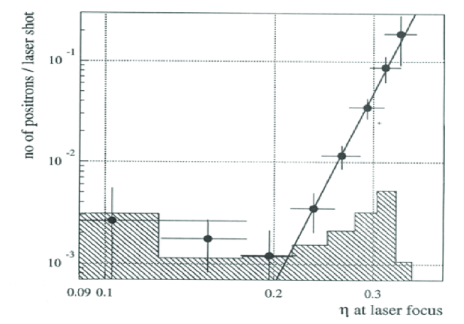
6.3.2 Pair production viewed in the rest frame of electron beam
In the reference frame where the electron beam is at rest, one can discuss [254] pair production in the processes (229) and (230) by using pair production rate Eqs. (353), (356), (359) in Section 6.2. In the experiment of colliding GeV electron beam with eV (nm) laser wave, the field strength in the laboratory is V/cm and intensity for [39]. The Lorentz gamma factor of the electron beam for GeV. In the rest frame of the electron beam, the electric field is given by
| (365) |
where laser’s electromagnetic fields , , , and laser’s wave vector , thus one has
| (366) |
The field of eV laser wave is well defined coherent wave field with wavelength cm and frequency /sec (the period sec). In the rest frame of electron beam, cm and sec. Comparing these wavelength and frequency of laser wave field with the spatial length cm and timescale sec of spontaneous pair production in vacuum, we are allowed to apply the homogeneous and adiabatic approximation discussed in Section 6.5.5, and use the rate of pair production (353), (356), (359) in Section 6.2.
6.4 The Breit–Wheeler cutoff in high-energy -rays
Having determined the theoretical basis as well as attempts to verify experimentally the Breit–Wheeler formula we turn to a most important application of the Breit–Wheeler process in the framework of cosmology. As pointed out by Nikishov [56] the existence of background photons in cosmology puts a stringent cutoff on the maximum trajectory of the high energy photons.
The Breit–Wheeler process for the photon-photon pair production is one of most relevant elementary processes in high-energy astrophysics. In addition to the importance of this process in dense radiation fields of compact objects [278], the essential role of this process in the context of intergalactic absorption of high-energy -rays was first pointed out by Nikishov [56, 279]. The spectra of TeV radiation observed from distant ( Mpc) extragalactic objects suffer essential deformation during the passage through the intergalactic medium, caused by energy-dependent absorption of primary -rays interacting with the diffuse extragalactic background radiation, for the optical depth most likely significantly exceeding one [279, 280, 281, 282]. A relevant broad-band information about the cosmic background radiation (CBR) is important for the interpretation of the observed high-energy spectra [283, 284, 285, 286]. For details, readers are referred to Refs. [287, 288]. In this section, we are particularly interested in such absorption effect of high-energy -ray, originated from cosmological sources, interacting with the Cosmic Microwave Background (CMB) photons. Fazio and Stecker [289, 290] were the first who calculated the cutoff energy versus redshift for cosmological -rays. This calculation was applied to further study of the optical depth of the Universe to high-energy -rays [291, 292, 293]. With the Fermi telescope, such study turns out to be important to understand the spectrum of high-energy -ray originated from sources at cosmological distance, we therefore offer the details of theoretical analysis as follow [294].
We study the Breit–Wheeler process (3) in the case that high-energy photons , originated from sources at cosmological distance , on their way to us, collide with CMB photons in the rest frame of CMB photons, leading to electron–positron pair production. We calculate the opacity and mean free path of these high-energy photons, find the energy range of absorption as a function of the cosmological redshift .
In general, a high-energy photon with a given energy , collides with background photons having all possible energies . We assume that -type background photons have the spectrum distribution , the opacity is then given by
| (367) |
where is the energy threshold (22) above which the Breit–Wheeler process (3) can occur and the cross-section is given by Eqs. (23); is the Hubble function, obeyed the Friedmann equation
| (368) |
We will assume and and Km/s/Mpc. The total opacity is then given by
| (369) |
which the sum is over all types of photon backgrounds in the Universe.
In the case of CMB photons the ir distribution is black-body one with the CMB temperature , the opacity is given by
| (370) |
where the Boltzmann constant . To simply Eq. (370), we set . In terms of CMB temperature and high-energy photons energy at the present time,
| (371) |
we obtain,
| (372) |
where
| (373) |
and is the energy in unit of eV.
The gives the relationship that separates the optically thick and optically thin regimes in the plane.

The integral (372) is evaluated numerically and the result is presented in Fig. 14. It clearly shows the following properties:
-
1.
for the redshift smaller than a critical value (), the CMB is transparent to photons with arbitrary energy, this indicates a minimal mean free path of high-energy photons;
-
2.
for the redshift larger than the value (), there are two branches of solutions for , respectively corresponding to the different energy dependence of the cross-section (23): the cross-section increases with the center of mass energy from the energy threshold to , and decreases (24) from to . The energy of the CMB photon corresponding to the critical redshift is eV which separates two branches of the solution. The position of this point in Fig. 14 is determined by the maximal cross-section at . Due to existence of these two solutions for a given redshift , photons having energies in the grey region of Fig. 14 cannot reach the observer, while photons from the white region of Fig. 14 are observable.
-
3.
above the critical redshift low-energy photons can reach us since their energies are smaller than the energetic threshold for the Breit–Wheeler process (3). In addition, high-energy photons are also observable due to the fact that the cross-section of Breit–Wheeler process (3) decreases with increasing energy of photons. For large redshifts , the Universe is opaque and we disregard this regime.
In Section 4.4 we considered another relevant process which is double pair production (121). This process contributes to the opacity at very high energies and its effect has been computed in [295]. We also computed the effect of this process on our diagram in Fig. 14. This process becomes relevant at very high redshift .
Due to the fact that there are other radiation backgrounds contributing into (369), the background of CMB photons gives the lower limit for opacity for high-energy photons with respect to the Breit–Wheeler process (3). Finally, we point out that the small-energy solution for large redshift in Fig. (14) agrees with the one found by Fazio and Stecker [289, 290].
6.5 Theory of pair production in Coulomb potential
By far the major attention to build a critical electric field has occurred in the physics of heavy nuclei and in heavy-ion collisions. We recall in the following some of the basic ideas, calculations, as well as experimental attempts to obtain the pair creation process in nuclear physics.
6.5.1 The catastrophe
Soon after the Dirac equation for a relativistic electron was discovered [80, 296], Gordon [297, 298] (for all ) and Darwin [299] (for ) found its solution in the point-like Coulomb potential . Solving the differential equations for the Dirac wave function, they obtained the well-known Sommerfeld’s formula [300] for the energy spectrum,
| (374) |
Here the principle quantum number and
| (375) |
where is the orbital angular momentum corresponding to the upper component of Dirac bi-spinor, is the total angular momentum, and the states with are doubly degenerate888This degeneracy is removed by radiative corrections [133, 90]. The shift of the level up, compared to the level (the famous Lamb shift) was discovered out of the study of fine structure of the hydrogen spectrum., while the state is a singlet [297, 298, 299]. The integer values and label bound states whose energies are . For the example, in the case of the lowest-energy states, one has
| (376) | |||||
| (377) | |||||
| (378) |
For all states of the discrete spectrum, the binding energy increases as the nuclear charge increases, as shown in Fig. 15. When , , and . Gordon noticed in his pioneer paper [297, 298] that no regular solutions with and (the ground state) are found beyond . This phenomenon is the so-called “ catastrophe” and it is associated with the assumption that the nucleus is point-like in calculating the electronic energy spectrum.

In fact, it was shown since the pioneering work of Pomeranchuk [64] that in nature there cannot be a point-like charged object with effective coupling constant since the entire electron shell will collapse to the center .
6.5.2 Semi-Classical description
In order to have further understanding of this phenomenon, we study it in the semi-classical scenario. For simplicity we treat relativistic electron as a scalar particle fulfilling the Klein–Gordon equation, but still obeying Fermi-Dirac statistics. Setting the origin of spherical coordinates at the point-like charge, we introduce the vector potential , where and is the Coulomb potential. The motion of a relativistic “electron” with mass and charge is described by its radial momentum , angular momenta and the Hamiltonian
| (379) |
where the potential energy , and corresponds for positive and negative solutions. The states corresponding to negative energy solutions are fully occupied. The angular momentum is conserved, when the Hamiltonian is spherically symmetric. For a given angular momentum , the Hamiltonian (379) describes electron’s radial motion in the following effective potential
| (380) |
The Coulomb potential energy is given by
| (381) |
In the classical scenario, given different values of angular momenta , the stable circulating orbits (states) are determined by the minimum of the effective potential (380). Using , we obtain the stable orbit location at the radius in the unit of the Compton length ,
| (382) |
where and . Substituting Eq. (382) into Eq. (380), we find the energy of the electron at each stable orbit,
| (383) |
The last stable orbits (minimal energy) are given by
| (384) |
For stable orbits with , the radii and energies ; electrons in these orbits are critically bound since their binding energy goes to zero. As the energy spectrum (374), see Eqs. (376,377,378), Eq. (383) shows, only positive or null energy solutions (states) exist in the presence of a point-like nucleus.
In the semi-classical scenario, the discrete values of angular momentum are selected by the Bohr-Sommerfeld quantization rule
| (385) |
describing the semi-classical states of radius and energy
| (386) | |||||
| (387) |
Other values of angular momentum , radius and energy given by Eqs. (382,383) in the classical scenario are not allowed. When these semi-classical states are not occupied as required by the Pauli Principle, the transition from one state to another with different discrete values ( and ) is possible by emission or absorption of a spin-1 () photon. Following the energy and angular-momentum conservations, photons emitted or absorbed in the transition have angular momentum and energy . As required by the Heisenberg uncertainty principle , the absolute ground state for minimal energy and angular momentum is given by the state, , and for . Thus the stability of all semi-classical states is guaranteed by the Pauli principle. In contrast for , there is not an absolute ground state in the semi-classical scenario.
We see now how the lowest-energy states are selected by the quantization rule in the semi-classical scenario out of the last stable orbits (384) in the classical scenario. For the case of , equating (384) to (385), we find the selected state is only possible solution so that the ground state in the semi-classical scenario corresponds to the last stable orbits (384) in the classical scenario. On the other hand for the case , equating (384) to (385), we find the selected state in the semi-classical scenario corresponds to the last stable orbits (384) in the classical scenario. This state is not protected by the Heisenberg uncertainty principle from quantum mechanically decaying in -steps to the states with lower angular momentum and energy (correspondingly smaller radius (386)) via photon emissions. This clearly shows that the “-catastrophe” corresponds to , falling to the center of the Coulomb potential and all semi-classical states () are unstable.
6.5.3 The critical value of the nuclear charge
A very different situation is encountered when considering the fact that the nucleus is not point-like and has an extended charge distribution [64, 301, 302, 303, 304, 305, 306, 307, 65]. In that case the catastrophe disappears and the energy levels of the bound states , and , smoothly continue to drop toward the negative energy continuum as increases to values larger than , as shown in Fig. 15. The reason is that the finite size of the nucleus charge distribution provides a cutoff for the boundary condition at the origin and the energy levels of the Dirac equation are shifted due to this cutoff. In order to determine the critical value when the negative energy continuum () is encountered (see Fig. 15), Zeldovich and Popov[304, 305, 306, 307, 65] solved the Dirac equation corresponding to a nucleus of finite extended charge distribution, i.e., the Coulomb potential is modified as
| (388) |
where cm is the size of the nucleus. The form of the cutoff function depends on the distribution of the electric charge over the volume of the nucleus , with . Thus, corresponds to a constant volume density of charge.
Solving the Dirac equation with the modified Coulomb potential (388) and calculating the corresponding perturbative shift of the lowest-energy level (376) Popov obtains[304, 65]
| (389) |
where , and is a logarithmic parameter in the problem under consideration. The asymptotic expressions for the energy that were obtained are[307, 65]
| (390) |
As a result, the “ catastrophe” in Eq. (374) disappears and gives
| (391) |
the state energy continuously goes down to the negative energy continuum since , and gives
| (392) |
as shown in Fig. 15. In Ref. [304, 65] Popov and Zeldovich found that the critical value for the energy levels and reaching the negative energy continuum is equal to
| (393) |
The critical value increases rapidly with increasing . As a result, it is found that is a critical value at which the lowest-energy level of the bound state encounters the negative energy continuum, while other bound states encounter the negative energy continuum at (see also Ref. [302] for a numerical estimation of the same spectrum). The change in the vacuum polarization near a high-Z nucleus arising from the finite extent of the nuclear charge density was computed in [308, 309, 310] with all calculations done analytically, and to all orders in . Note that for two nuclei with charges and respectively, if and -shell of the -nucleus is empty, then may be a neutral atom. In this case two nuclei make a quasimolecular state for which the ground term is unoccupied by electrons: so spontaneous production of positrons is also possible [311, 312]. We refer the readers to Ref. [304, 305, 306, 307, 65, 313] for mathematical and numerical details.
When , the lowest-energy level of the bound state enters the negative energy continuum. Its energy level can be estimated as follows
| (394) |
where is the average radius of the state’s orbit, and the binding energy of this state satisfies . If this bound state is unoccupied, the bare nucleus gains a binding energy larger than , and becomes unstable against the production of an electron–positron pair. Assuming this pair production occurs around the radius , we have energies for the electron () and positron () given by
| (395) |
where are electron and positron momenta, and . The total energy required for the production of a pair is
| (396) |
which is independent of the potential . The potential energies of the electron and positron cancel out each other and do not contribute to the total energy (396) required for pair production. This energy (396) is acquired from the binding energy () by the electron filling into the bound state . A part of the binding energy becomes the kinetic energy of positron that goes out. This is analogous to the familiar case when a proton () catches an electron into the ground state , and a photon is emitted with the energy not less than 13.6 eV. In the same way, more electron–positron pairs are produced, when and the energy levels of the next bound states enter the negative energy continuum, provided these bound states of the bare nucleus are unoccupied.
6.5.4 Positron production
Gershtein and Zeldovich [314, 315] proposed that when the bare nucleus produces spontaneously pairs of electrons and positrons: the two positrons999Hyperfine structure of state: single and triplet. run off to infinity and the effective charge of the bare nucleus decreases by two electrons, which corresponds exactly to filling the K-shell101010An assumption was made in Ref. [314, 315] that the electron density of state, as well as the vacuum polarization density, is delocalized at . Later it was proved to be incorrect [305, 306, 65]. A more detailed investigation was made for the solution of the Dirac equation at , when the lowest electron level merges with the negative energy continuum, in Refs. [304, 305, 306, 307, 316]. It was there further clarified the situation, showing that at , an imaginary resonance energy of Dirac equation appears,
| (397) |
where
| (398) | |||||
| (399) |
and are constants, depending on the cutoff (for example, for [305, 306, 65]). The energy and momentum of emitted positrons are and .
The kinetic energy of the two positrons at infinity is given by
| (400) |
which is proportional to (as long as ) and tends to zero as . The pair production resonance at the energy (397) is extremely narrow and practically all positrons are emitted with almost same kinetic energy for , i.e. nearly mono-energetic spectra (sharp line structure). Apart from a pre-exponential factor, in Eq. (399) coincides with the probability of positron production, i.e., the penetrability of the Coulomb barrier (see Section 2.5). The related problems of vacuum charge density due to electrons filling into the K-shell and charge renormalization due to the change of wave function of electron states are discussed in Refs. [317, 318, 319, 320, 321]. An extensive and detailed review on this theoretical issue can be found in Refs. [65, 313, 322, 66].
On the other hand, some theoretical work has been done studying the possibility that pair production, due to bound states encountering the negative energy continuum, is prevented from occurring by higher order processes of quantum field theory, such as charge renormalization, electron self-energy and nonlinearities in electrodynamics and even Dirac field itself [222, 323, 324, 325, 326, 327, 328]. However, these studies show that various effects modify by a few percent, but have no way to prevent the binding energy from increasing to as increases, without simultaneously contradicting the existing precise experimental data on stable atoms [329]. Contrary claim [330] according to which bound states are repelled by the lower continuum through some kind of self-screening appear to be unfounded [66].
It is worth noting that an overcritical nucleus () can be formed for example in the collision of two heavy nuclei [303, 316, 314, 315, 331, 332, 333, 334]. To observe the emission of positrons originated from pair production occurring near to an overcritical nucleus temporally formed by two nuclei, the following necessary conditions have to be full filled: (i) the atomic number of an overcritical nucleus is larger than ; (ii) the lifetime of the overcritical nucleus must be much longer than the characteristic time of pair production; (iii) the inner shells (K-shell) of the overcritical nucleus should be unoccupied.
The collision of two Uranium nuclei with was considered by Zeldovich, Popov and Gershtein [65, 311]. The conservation of energy in the collision reads
| (401) |
where is the relative velocity of the nuclei at infinity, is the smallest distance, and is the Uranium atomic mass. In order to have fm a fine tuning of the initial velocity narrowly peaked around is needed. The characteristic collision time would be then s. The interesting possibility then occurs, that the typical velocity of an electron in the inner shell (fm) is and therefore its characteristic time s. This means that the characteristic collision time in which the two colliding nuclei are brought into contact and separated again can be in principle much larger than the timescale of electron evolution. This would give justification for an adiabatic description of the collision in terms of quasimolecules. The formation of “quasimolecules” could also be verified by the characteristic molecular-orbital X-rays radiation due to the electron transitions between “quasimolecules” orbits [329, 335, 336, 337, 338, 339, 340, 341]. However, this requires the above mentioned fine tuning in the bombarding energies () close to the nuclear Coulomb barrier.
However, we notice that the above mentioned condition (ii) has never been fulfilled in heavy-ion collisions. There has been up to now various unsuccessful attempts to broaden this time of encounter by ‘sticking’ phenomena. Similarly, the condition (iii) is not sufficient for pair production, since electrons that occupied outer shells of high energies must undergo a rapid transition to occupy inner shells of lower energies, which is supposed to be vacant and encountering the negative energy continuum. If such transition and occupation take place faster than pair production, the pair production process is blocked. As a consequence, it needs a larger value of to have stronger electric field for vacant out shells encountering the negative energy continuum (see Eq. (393)) so that electrons produced can occupy outer shells. This makes pair production even less probable to be observed, unless the overcritical charged nucleus is bare, i.e. all shells are vacant.
6.5.5 Homogeneous and adiabatic approximation
There is a certain analogy between positron production by a nucleus with and pair production in a homogeneous electrostatic field. We note that in a Coulomb potential of a nucleus with the corresponding electric field is comparable with the critical electric field , (1), when . However, the condition is certainly the necessary condition in order to have the pair creation but not a sufficient one: the spatial extent of the region where occurs must be larger than the de Broglie wavelength of the created electron—positron pair. If a pair production takes place, electrons should be bound into the K-shell nucleus and positrons should run off to infinity. This intuitive reasoning builds the connection between the phenomena of pair production in the Coulomb potential at charge and the one in an external constant electric field which was treated in Section 4.7. The exact formula for pair production probability in an overcritical Coulomb potential has not yet been obtained in the framework of QED. We cannot expect a literal coincidence of formulas for the probability of pair production in these different cases, since the Schwinger formula (160) is exactly derived for a homogeneous field, while the Coulomb potential is strongly inhomogeneous at small distances. Some progress in the treatment of this problem is presented in Section 5.
All the discussions dealing with pair production in an external homogeneous electric field or a Coulomb potential assume that the electric field be static. Without the feedback of the particles created on the field this will clearly lead to a divergence of the number of pairs created. In the real description of the phenomenon at we have an initial empty vacuum state. We then have the turned on of an overcritical electric field and ongoing process of pair creation with their feedback on a time on the electric field and a final state at remote future with the electron and positron created and the remaining subcritical electric field. To describe this very different regimes a simplified “adiabatic approximation” can be adopted by assuming the existence of a homogeneous field only during a finite time interval . That time should be of course shorter than the feedback time . During that time interval the Schwinger formula (160) is assumed to be applicable and it is appropriate to remark that the overcritical electric fields are related to very high energy densities: ergs/cm3. In the adiabatic approximation an effective spatial limitation to the electric field is also imposed. Therefore the constant overcritical electric field and the application of the Schwinger formula is limited both in space and time. Progress in this direction has been presented in [73], see Section 8.8. A significant amount of pairs is only produced if the finite lifetime of the overcritical electric field is larger than the characteristic time of pair production () and the spatial extent of the electric field is larger than the tunneling length (52).
We have already discussed in Secs. 6.2 and 6.3 the experimental status of electron–positron pair creation in X-ray free electron laser and an electron-beam–laser collision, respectively. We now turn in Section 6.6 to the multiyear attempts in creating electron–positron pairs in heavy-ion collisions.
6.6 Pair production in heavy-ion collisions
6.6.1 A transient super heavy “quasimolecules”
There has been a multiyear effort to observe positrons from pair production associated with the overcritical field of two colliding nuclei, in heavy-ion collisions [316, 329, 314, 315, 333, 334, 342]. The hope was to use heavy-ion collisions to form transient superheavy “quasimolecules”: a long-lived metastable nuclear complex with . It was expected that the two heavy ions of charges respectively and with would reach small inter-nuclear distances well within the electron’s orbiting radii. The electrons would not distinguish between the two nuclear centers and they would evolve as if they were bounded by nuclear “quasimolecules” with nuclear charge . Therefore, it was expected that electrons would evolve quasi-statically through a series of well defined nuclear “quasimolecules” states in the two-center field of the nuclei as the inter-nuclear separation decreases and then increases again.
When heavy-ion collision occurs the two nuclei come into contact and some deep inelastic reaction occurs determining the duration of this contact. Such “sticking time” is expected to depend on the nuclei involved in the reaction and on the beam energy. Theoretical attempts have been proposed to study the nuclear aspects of heavy-ion collisions at energies very close to the Coulomb barrier and search for conditions, which would serve as a trigger for prolonged nuclear reaction times, to enhance the amplitude of pair production. The sticking time should be larger than sec [66] in order to have significant pair production, see Fig. 16. Up to now no success has been achieved in justifying theoretically such a long sticking time. In reality the characteristic sticking time has been found of the order of sec, hundred times shorter than the one needed to activate the pair creation process. Moreover, it is recognized that several other dynamical processes can make the existence of a sharp line corresponding to an electron–positron annihilation very unlikely [66, 329, 343, 344, 345].

It is worth noting that several other dynamical processes contribute to the production of positrons in undercritical as well as in overcritical collision systems [323, 324, 222, 325]. Due to the time-energy uncertainty relation (collision broadening), the energy spectrum of such positrons has a rather broad and oscillating structure, considerably different from a sharp line structure that we would expect from pair production positron emission alone.
6.6.2 Experiments
As remarked above, if the sticking time could be prolonged, the probability of pair production in vacuum around the superheavy nucleus would be enhanced. As a consequence, the spectrum of emitted positrons is expected to develop a sharp line structure, indicating the spontaneous vacuum decay caused by the overcritical electric field of a forming superheavy nuclear system with . If the sticking time is not long enough and the sharp line of pair production positrons has not yet well developed, in the observed positron spectrum it is difficult to distinguish the pair production positrons from positrons created through other different mechanisms. Prolonging the “sticking time” and identifying pair production positrons among all other particles [346, 335] created in the collision process has been an object of a very large experimental campaign [347, 348, 349, 350, 351, 352, 353, 354].
For nearly 20 years the study of atomic excitation processes and in particular of positron creation in heavy-ion collisions has been a major research topic at GSI (Darmstadt) [355, 356, 357, 358]. The Orange and Epos groups at GSI (Darmstadt) discovered narrow line structures (see Fig. 17) of unexplained origin, first in the single positron energy spectra and later in coincident electron–positron pair emission. Studying more collision systems with a wider range of the combined nuclear charge they found that narrow line structures were essentially independent of . This has ruled out the explanation as a pair production positron, since the line was expected to be at the position of the resonance, i.e., at a kinetic energy given by Eq. (400), which is strongly dependent. Attempts to link this positron line to spontaneous pair production have failed. Other attempts to explain this positron line in term of atomic physics and new particle scenario were not successful as well [66].
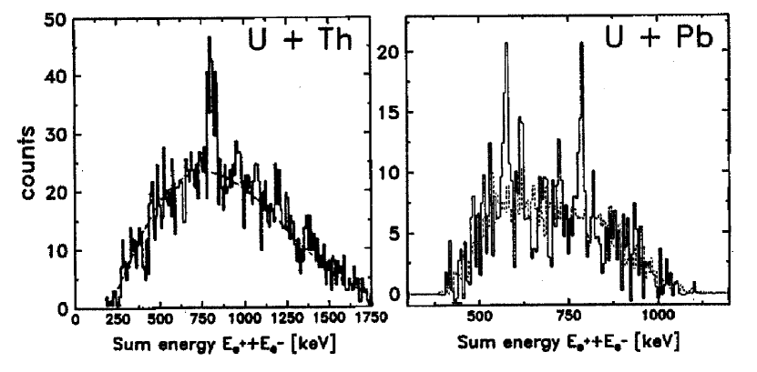
The anomalous positron line problem has perplexed experimentalists and theorists alike for more than a decade. Moreover, later results obtained by the Apex collaboration at Argonne National Laboratory showed no statistically significant positron line structures [359, 360]. This is in strong contradiction with the former results obtained by the Orange and Epos groups. However, the analysis of Apex data was challenged in the comment by Ref. [361, 362] pointing out that the Apex measurement would have been less sensitive to extremely narrow positron lines. A new generation of experiments (Apex at Argonne and the new Epos and Orange setups at GSI) with much improved counting statistics has failed to reproduce the earlier results [66].
To overcome the problem posed by the short timescale of pair production ( sec), hopes rest on the idea to select collision systems in which a nuclear reaction with sufficient sticking time occurs. Whether such a situation can be realized still is an open question [66]. In addition, the anomalous positron line problem and its experimental contradiction overshadow the field of the pair production in heavy-ion collisions.
In summary, clear experimental signals for electron–positron pair production in heavy-ion collisions are still missing [66] at the present time. For more recent information on the pair production in the heavy-ion collisions see [363, 364, 365] and for complete references the resource letter [366].
Having reviewed the situation of electron–positron pair creation by vacuum polarization in Earth-bound experiments we turn now to the corresponding problems in the realm of astrophysics. The obvious case is the one of black holes where the existence of critical field is clearly predicted by the analytic solutions of the Einstein-Maxwell field equations.
7 The extraction of blackholic energy from a black hole by vacuum polarization processes
It is becoming more and more clear that the theoretical description of the gravitational collapse process to a Kerr–Newman black hole, with all the aspects of nuclear physics and electrodynamics involved, is likely the most complex problem in physics and astrophysics. Specific to this report is the opportunity given by the process of gravitational collapse to study for the first time the above mentioned three quantum processes simultaneously at work under ultrarelativistic special and general relativistic regimes. The process of gravitational collapse is characterized by the gravitational timescale sec, where is the gravitational constant, is the mass of a collapsing object, and the energy involved is of the order of ergs. This is one of the most energetic and most transient phenomena in physics and astrophysics and needs for its correct description the identification of the basic constitutive processes occurring in a highly time varying regime. Our approach in this Section is to proceed with an idealized model which can give us estimates of the basic energetics and some leading features of the real phenomenon. We shell describe: (1) the basic energetic process of an already formed black hole; (2) the vacuum polarization process a la Schwinger of an already formed Kerr–Newman black hole; (3) the basic formula of the dynamics of the gravitational collapse. We shall in particular recover the Tolman-Oppenheimer-Snyder solutions in a more explicit form and give exact analytic solution for the description of the gravitational collapse of charged and uncharged shells. This will allow, among others, to recall the mass formula of the black hole, to clarify the special role of the irreducible mass in that formula, and to have a general derivation of the maximum extractable energy in the process of gravitational collapse. We will as well address some conceptual issues between general relativity and thermodynamics which have been of interest to theoretical physicists in the last forty years. Of course in this brief Section we will be only recalling some of these essential themes and refer to the literature where in-depth analysis can be found. Since we are interested in the gravitational collapse we are going to examine only processes involving masses larger than the critical mass of neutron stars, for convenience established in 3.2 [367]. We are consequently not addressing the research on mini-black-holes [368] which involves energetics times smaller than the ones involved in gravitational collapse and discussed in this report. This problematics implies a yet unknown physics of applying quantum mechanics in conditions where the curvature of space-time is comparable to the wavelength of the particle.
We recall here the basic steps leading to the study of the electrodynamics of a Kerr–Newman black hole, indicating the relevant references. In this Section we use the system of units .
7.1 Test particles in Kerr–Newman geometries
According to the uniqueness theorem for stationary, regular black holes (see Ref. [369]), the process of gravitational collapse of a core whose mass is larger than the neutron star critical mass [367] will generally lead to a black hole characterized by all the three fundamental parameters: the mass-energy , the angular momentum , and the charge (see [370]). The creation of critical electric fields and consequent process of pair creation by vacuum polarization are expected to occur in the late phases of gravitational collapse when the gravitational energy of the collapsing core is transformed into an electromagnetic energy and eventually in electron–positron pairs. As of today no process of the gravitational collapse either to a neutron star or to a black hole has reached a satisfactory theoretical understanding. It is a fact that even the theory of a gravitational collapse to a neutron star via a supernova is not able to explain even the ejection of a supernova remnant [371]. In order to estimate the fundamental energetics of these transient phenomena we recall first the metric of a Kerr–Newman black hole, the role of the reversible and irreversible transformations in reaching the mass formula as well as the role of the positive and negative energy states in a quantum analog. We will then estimate the energy emission due to vacuum polarization process. As we will see, such a process occurs on characteristic quantum timescale of sec, which is many orders of magnitude shorter than the characteristic gravitational collapse timescale. Of course the astrophysical progenitor of the black hole will be a neutral one, as all the astrophysical systems. Only during the process of the gravitational collapse and for the above mentioned characteristic gravitational timescale a process of charge separation will occur. The positively charged core would give rise to the electrodynamical process approaching asymptotically in time the horizon of a Kerr–Newman black hole.
A generally charged and rotating, black hole has been considered whose curved space-time is described by the Kerr–Newman geometry [372]. In Kerr–Newman coordinates the line element takes the form,
| (402) |
where and , being the angular momentum per unit mass of the black hole. The Reissner–Nordström and Kerr geometries are particular cases for a nonrotating, , and uncharged, , black holes respectively. The Kerr–Newman space–time has a horizon at
| (403) |
where .
The electromagnetic vector potential around the Kerr–Newman black hole is given by [372]
| (404) |
the electromagnetic field tensor is then
| (405) |
The equation of motion of a test particle of mass and charge in the Kerr–Newman geometry reads
| (406) |
where is the 4–velocity of the particle. These equations may be derived from the Lagrangian
| (407) |
or, equivalently, from the Hamiltonian
| (408) |
where we have introduced the 4–momentum of the particle
| (409) |
Note that Hamiltonian (408) is subject to the constraint
| (410) |
Carter [67] firstly recognized that the corresponding Hamilton–Jacobi equations
| (411) |
are separable. Correspondingly four integrals of the equation of motion (406) can be found. Indeed, in addition to the constant of motion (410) which corresponds to conservation of the rest mass we have the two first integrals
| (412) | ||||
| (413) |
associated with the stationarity and the axial symmetry of Kerr–Newman space-time respectively. and are naturally interpreted as the energy and the angular momentum about the symmetry axis of the test particle. It follows from the separability of Eq. (411) that the quantities
| (414) | ||||
| (415) |
are conserved as well. Together with and they form a complete set of first integrals of the motion and allow one to integrate Eq. (406). As an example consider the proper time derivative of the radial coordinate of the test particle. It follows from Eqs. (412), (413), (414) and (415), that
| (416) |
which can be numerically integrated using the effective potential technique [373].
7.2 Reversible and irreversible transformations of a black hole: the Christodoulou-Ruffini mass formula
In 1969 Roger Penrose [374] pointed out for the first time the possibility to extract rotational energy from a Kerr black hole. The first example of such an energy extraction was obtained by Ruffini and Wheeler who also introduced the concept of the ergosphere [375, 177, 370], the region between the horizon of the black hole and the surface of infinite redshift. These works has been generalized by Denardo and Ruffini in 1973 [376] and Denardo, Hively and Ruffini in 1974 [377] to the case of a Kerr–Newman black hole. The process described by Denardo, Hively and Ruffini can be described as follows. A neutral particle approaches the black hole with positive energy and decays into two oppositely charged particles and whose energies are and respectively. falls into the black hole while is accelerated towards spatial infinity. Correspondingly, a positive energy
| (417) |
has been extracted from the black hole and deposited on . The region around the black hole where the energy extraction processes can occur is named effective ergosphere in Refs. [376], [377]. Note that, as the particle is swallowed, the black hole undergoes a transformation since its energy, angular momentum and charge change accordingly. When is the extracted energy maximal? In order to answer this question note that the energy of a particle of angular momentum , charge and rest mass moving around a Kerr–Newman black hole and having a turning point at is given by (see Eq. (416)) the quadratic equation
| (418) |
As recalled in [114, p. 352], in the case of which corresponds to a pure Kerr solution, the explicit integration of this equation was performed by Ruffini and Wheeler [378]. They introduced the effective potential energy defined by
| (419) |
The radii of stable orbits are determined by minimum of function , i.e. by simultaneous solution of equations , for . The orbit closest to the center corresponds to ; for , the function has no minima. As a result
-
•
When (motion opposite to the direction of rotation of the collapsing object)
(420) -
•
For (motion in the direction of rotation of the collapsing object) as the radius tends towards the radius of the horizon. Setting , we find in the limit :
(421) Then
(422)
We call attention to the fact that remainsgreater than one throughout, i.e. the orbit does not go inside the horizon. This is as it should be: the horizon is a null hypersurface, and no time-like world lines of moving particles can lie on it. Although no general formula exists in the case of the Kerr–Newman geometry the energy and the angular velocity of a test particle in a circular orbit with radius in the Reissner–Nordström geometry has been given by Ruffini and Zerilli [373]
| (423) | |||||
and the limiting cases are there treated.
Eq. (418) is not only relevant for understanding the fully relativistic stable circular orbit but it also defines the “positive root states” and the “negative root states” for the particle [379]. Such states were first interpreted as limits of states of a quantum field by Deruelle and Ruffini [380]. Such an interpretation will be discussed in the next section. Note that in the case there can exist negative energy states of positive root solutions and, as a direct consequence, energy can be extracted from a Kerr–Newman black hole via the Denardo-Ruffini process. Such a process is most efficient when the reduction of mass is greatest for a given reduction in angular momentum. To meet this requirement the energy must be as negative as possible. This happens when , that is the particle has a turning point at the horizon of the black hole. When , and the separation between negative and positive root states vanishes. This implies that capture processes from such an orbit are reversible since they can be inverted bringing the black hole to its original state. Correspondingly the energy of the incoming particle is
| (425) |
If we apply the conservation of energy, angular momentum and charge to the capture of the particle by the black hole, we find that , and change as for the quantities
| (426) |
Thus Eq. (425) reads
| (427) |
Integration of Eq. (427) gives
| (428) |
provided the condition is satisfied
| (429) |
where is an integration constant and we restored the physical constants and . Eq. (428) is the Christodoulou–Ruffini mass formula [379] and it expresses the contributions to the total energy of the black hole. Extreme black holes satisfy equality (429). The irreducible mass satisfies the equation [379]
| (430) |
where is the surface area of the horizon of the black hole, and cannot be decreased by classical processes. Any transformation of the black hole which leaves fixed the irreducible mass (for instance, as we have seen, the capture of a particle having a turning point at the horizon of the black hole) is called reversible [379]. Any transformation of the black hole which increases its irreducible mass, for instance, the capture of a particle with nonzero radial momentum at the horizon, is called irreversible. In irreversible transformations there is always some kinetic energy that is irretrievably lost behind the horizon. Note that energy can be extracted approaching arbitrarily close to reversible transformations which are the most efficient ones. Namely, from Eq. (428) it follows that up to 29 of the mass-energy of an extreme Kerr black hole () can be stored in its rotational energy term and can in principle be extracted. Gedankenexperiments have been conceived to extract such energy [374, 381, 382, 383, 384]. The first specific example of a process of energy extraction from a black hole can be found in R. Ruffini and J. A. Wheeler, as quoted in [385], see also [386]. Other processes of rotational energy extraction of astrophysical interest based on magnetohydrodynamic mechanism occurring around a rotating Black Hole have also been advanced [381, 382, 383, 384] though their reversibility as defined in Ref. [379], and consequently their efficiency of energy extraction, has not been assessed. From the same mass formula (428) follows that up to 50 of the mass energy of an extreme black hole with can be stored in the electromagnetic term and can be in principle extracted. These extractable energies either rotational or electromagnetic will be indicated in the following as blackholic energy and they can be the source of some of the most energetic phenomena in the Universe like jets from active galactic nuclei and GRBs.
7.3 Positive and negative root states as limits of quantum field states
In 1974 Deruelle and Ruffini [380] pointed out that negative root solutions of Eq. (418) can be interpreted in the framework of a fully relativistic quantum field theory as classical limits of antimatter solutions. In this section we briefly review their analysis. The equation of motion of a test particle in a Kerr–Newman geometry can be derived by the Hamilton–Jacobi Eq. (411). The first quantization of the corresponding theory can be obtained by substituting the Hamilton–Jacobi equation with the generalized Klein–Gordon equation
| (431) |
for the wave function . For simplicity we restrict to the Kerr case: , when Eq. (431) reduces to
| (432) |
In order to solve Eq. (432) we can separate the variables as follows:
| (433) |
where are spheroidal harmonics. We thus obtain the radial equation
where and . It is natural to look for “resonances” states of the Klein–Gordon equation corresponding to classical bound states (circular or elliptic orbits). Then, impose as boundary conditions (a) an exponential decay of the wave function for and (b) a purely ingoing wave at the horizon . The solutions of the corresponding problem can be found numerically [380]. The main conclusions of the integration can be summarized as follows:
-
1.
The continuum spectrum of the classical stable bound states is replaced by a discrete spectrum of resonances with tunneling through the potential barrier giving the finite probability of the particle to be captured by the horizon.
-
2.
In the classical limit the separation of the energy levels of the resonances tends to zero. The leakage toward the horizon also decreases and the width of the resonance tends to zero.
-
3.
The negative root solutions of Eq. (418) correspond to the classical limit of the negative energy solutions of the Klein–Gordon Eq. (432) and consequently they can be thought of as antimatter solutions with an appropriate interchange of the sign of charge, the direction of time and the angular momentum.
-
4.
We can have positive root states of negative energy in the ergosphere, see e.g. [375]. In particular we can have crossing of positive and negative energy root states. This corresponds, at the second quantized theory level to the possibility of particle pair creation à là Klein, Sauter, Heisenberg, Euler and Schwinger [17, 18, 20, 7, 25, 26, 27].
Similar considerations can be made in the Kerr–Newman case, , when the generalized Klein Gordon Eq. (431) has to be integrated. The resonance states can be obtained imposing the same boundary conditions as above. Once again we can have level crossing inside the effective ergosphere [376, 377] and therefore possible pair creation.
7.4 Vacuum polarization in Kerr–Newman geometries
We discussed in the previous Sections the phenomenon of electron–positron pair production in a strong electric field in a flat space-time. Nere we study the same phenomenon occurring around a black hole endowed with mass , charge and the angular momentum .
The space-time of a Kerr–Newman geometry is described by a metric which in Boyer–Lindquist coordinates acquires the form
| (434) |
where and are defined following (402). We recall that the Reissner–Nordstrøm geometry is the particular case of a nonrotating black hole.
The electromagnetic vector potential around the Kerr–Newman black hole is given in Boyer–Lindquist coordinates by
| (435) |
The electromagnetic field tensor is then
| (436) |
After some preliminary work in Refs. [387, 388, 389], the occurrence of pair production in a Kerr–Newman geometry was addressed by Deruelle [390]. In a Reissner–Nordström geometry, QED pair production has been studied by Zaumen [391] and Gibbons [392]. The corresponding problem of QED pair production in the Kerr–Newman geometry was addressed by Damour and Ruffini [68], who obtained the rate of pair production with particular emphasis on:
-
•
the limitations imposed by pair production on the strength of the electromagnetic field of a black hole [373];
-
•
the efficiency of extracting rotational and Coulomb energy (the “blackholic” energy) from a black hole by pair production;
-
•
the possibility of having observational consequences of astrophysical interest.
In the following, we recall the main results of the work by Damour and Ruffini.
In order to study the pair production in the Kerr–Newman geometry, they introduced at each event a local Lorentz frame associated with a stationary observer at the event . A convenient frame is defined by the following orthogonal tetrad [67]
| (437) | ||||
| (438) | ||||
| (439) | ||||
| (440) |
In this Lorentz frame, the electric potential , the electric field and the magnetic field are given by the following formulas (c.e.g. Ref. [393]),
We then obtain
| (441) |
while the electromagnetic fields and are parallel to the direction of and have strengths given by
| (442) | ||||
| (443) |
respectively. The maximal strength of the electric field is obtained in the case at the horizon of the black hole: . We have
| (444) |
In the original paper a limit on the black hole mass was established by requiring that the pair production process would last less than the age of the Universe. For masses much smaller than this absolute maximum mass the pair production process can drastically modify the electromagnetic structure of black hole.
Both the gravitational and the electromagnetic background fields of the Kerr–Newman black hole are stationary when considering the quantum field of the electron. Since the gravitational field of the background black hole is practically constant over the Compton wavelength of the electron characterizing the quantum field. As far as purely QED phenomena such as pair production are concerned, it is possible to consider the electric and magnetic fields defined by Eqs. (442,443) as constants in the neighborhood of a few wavelengths around any events . Thus, the analysis and discussion on the Sauter-Euler-Heisenberg-Schwinger process over a flat space-time can be locally applied to the case of the curved Kerr–Newman geometry, based on the equivalence principle.
The rate of pair production around a Kerr–Newman black hole can be obtained from the Schwinger formula (174) for parallel electromagnetic fields and as:
| (445) |
The total number of pairs produced in a region of the space-time is
| (446) |
where . In Ref. [68], it was assumed that for each created pair the particle (or antiparticle) with the same sign of charge as the black hole was expelled to infinity with charge , energy and angular momentum while the antiparticle was absorbed by the black hole. This implies the decrease of charge, mass and angular momentum of the black hole and a corresponding extraction of all three quantities. These considerations, however, were profoundly modified later by the introduction of the concept of dyadosphere which is presented in the next section. The rates of change of the charge, mass and angular momentum were estimated by
| (447) | ||||
where is the rate of pair production and and represent some suitable mean values for the energy and angular momentum carried by the pairs.
Supposing the maximal variation of black hole charge to be , one can estimate the maximal number of pairs created and the maximal mass-energy variation. It was concluded in Ref. [68] that the maximal mass-energy variation in the pair production process is larger than erg and up to erg, depending on the black hole mass, see Table 1 in [68]. They concluded at the time “this work naturally leads to a most simple model for the explanation of the recently discovered -ray bursts”.
7.5 The “Dyadosphere” in Reissner–Nordström geometry
After the discovery in 1997 of the afterglow of GRBs [394] and the determination of the cosmological distance of their sources, at once of the order of theories explaining them were wiped out on energetic grounds. On the contrary, it was noticed [395, 396] the coincidence between their observed energetics and the one theoretically predicted by Damour and Ruffini [68] of ergs per burst for . Ruffini and collaborators therefore, indirectly motivated by GRBs, returned to these theoretical results with renewed interest developing some additional basic theoretical concepts [395, 397, 398, 399, 400, 401, 402] such as the dyadosphere and, more recently, the dyadotorus. In this Section we restore constants , and for clarity.
As a first simplifying assumption the case of absence of rotation was considered. The space-time is then described by the Reissner–Nordström geometry, see (434) whose spherically symmetric metric is given by
| (448) |
where and .
The first result obtained is that the pair creation process does not occur at the horizon of the black hole: it extends over the entire region outside the horizon in which the electric field exceeds the value of the order of magnitude of the critical value given by Eq. (1). We recall the pair creation process is a quantum tunneling between the positive and negative energy states, which needs a level crossing, can occur for as well, if the field extent to spatial dimension such that . The probability of such pair creation process will be exponentially damped by . Clearly, very intense process of pair creation will occur for . In order to give a scale of the phenomenon, and for definiteness, in Ref. [398] it was considered the case of , although later in order to take into due account the tunneling effects we have considered dyadosphere for electric field in the range
| (449) |
with in the range 0.1-10. Since the electric field in the Reissner–Nordström geometry has only a radial component given by [403]
| (450) |
this region extends from the horizon radius, for
| (451) |
out to an outer radius [395]
| (452) |
where we have introduced the dimensionless mass and charge parameters , , see Fig. 19.
The second result gave the local number density of electron and positron pairs created in this region as a function of radius
| (453) |
and consequently the total number of electron and positron pairs in this region is
| (454) |
where .

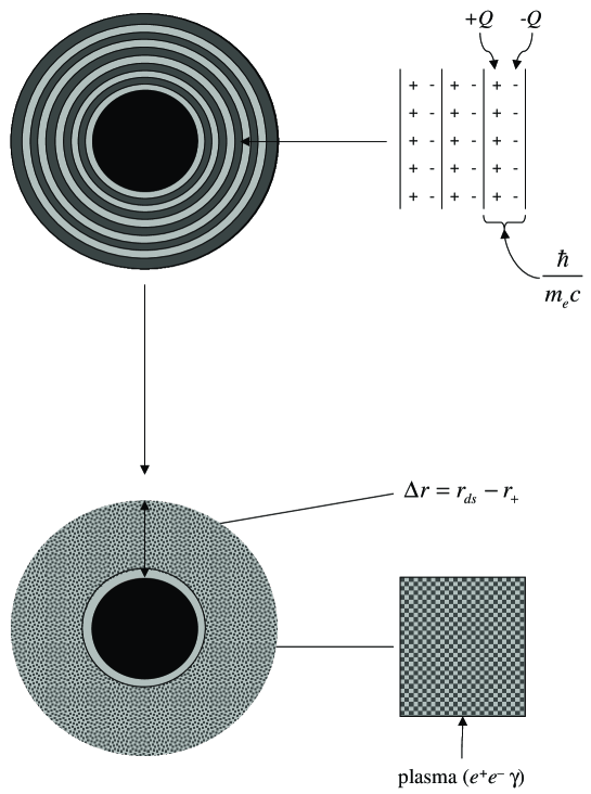
The total number of pairs is larger by an enormous factor than the value which a naive estimate of the discharge of the black hole would have predicted. Due to this enormous amplification factor in the number of pairs created, the region between the horizon and is dominated by an essentially high density neutral plasma of electron–positron pairs. This region was defined [395] as the dyadosphere of the black hole from the Greek duas, duados for pairs. Consequently we have called the dyadosphere radius [395, 397, 398]. The vacuum polarization process occurs as if the entire dyadosphere is subdivided into a concentric set of shells of capacitors each of thickness and each producing a number of pairs on the order of (see Fig. 19). The energy density of the electron–positron pairs is there given by
| (455) |
(see Figs. 2–3 of Ref. [397]). The total energy of pairs converted from the static electric energy and deposited within the dyadosphere is then
| (456) |
In the limit , Eq. (456) leads to , which coincides with the energy extractable from black holes by reversible processes (), namely [379], see Fig. 18. Due to the very large pair density given by Eq. (453) and to the sizes of the cross-sections for the process , the system has been assumed to thermalize to a plasma configuration for which
| (457) |
where is the total number density of -pairs created in the dyadosphere [397, 398].
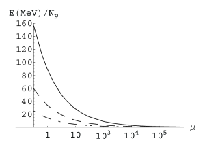
In Fig. 20 we show the average energy per pair as a function of the black hole mass in solar mass units [398]. This assumption has been in the meantime rigorously proven by Aksenov, Ruffini and Vereshchagin [74], see Section 9.
The third result, again introduced for simplicity, is that for a given it was assumed either a constant average energy density over the entire dyadosphere volume, or a more compact configuration with energy density equal to its peak value. These are the two possible initial conditions for the evolution of the dyadosphere (see Fig. 21).


The above theoretical results permit a good estimate of the general energetics processes originating in the dyadosphere, assuming an already formed black hole and offer a theoretical framework to estimate the general relativistic effect and characteristic time scales of the approach to the black hole horizon [405, 406, 407, 408, 409, 410].
7.6 The “dyadotorus”
We turn now to examine how the presence of rotation modifies the geometry of the surface containing the region where electron–positron pairs are created as well as the conditions forthe existence of such a surface. Due to the axial symmetry of the problem, this region was called the “dyadotorus” [411, 412].
We shall follow the treatment of [411, 412]. As in Damour [413, 383] we introduce at each point of the space-time the orthogonal Carter tetrad (437-440).
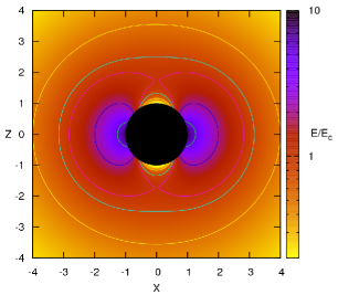
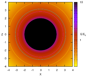
From Eq. (442) we define the dyadotorus by the condition , where , see Fig. 22. Solving for and introducing the dimensionless quantities , , , and we get
| (458) |
where the signs correspond to the two different parts of the surface.
The two parts of the surface join at the particular values and of the polar angle where
The requirement that can be solved for instance for the charge parameter , giving a range of values of for which the dyadotorus takes one of the shapes (see fig.23)
| (459) |
where .
In Fig. 23 we show some examples of the dyadotorus geometry for different sets of parameters for an extreme Kerr–Newman black hole (), we can see the transition from a toroidal geometry to an ellipsoidal one depending on the value of the black hole charge.
Fig. 24 shows the projections of the surfaces corresponding to different values of the ratio for the same choice of parameters as in Fig. 23 (b), as an example. We see that the region enclosed by such surfaces shrinks for increasing values of .
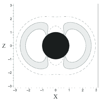
7.7 Geometry of gravitationally collapsing cores
In the previous Sections we have focused on the theoretically well defined problem of pair creation in the electric field of an already formed black hole. In this section we shall follow the treatment of Cherubini et al. [405] addressing some specific issues on the dynamical formation of the black hole, recalling first the Oppenheimer-Snyder solution and then considering its generalization to the charged case using the classical work of W. Israel and V. de la Cruz [70, 71].
7.7.1 The Tolman-Oppenheimer-Snyder solution
Oppenheimer and Snyder first found a solution of the Einstein equations describing the gravitational collapse of spherically symmetric star of mass greater than . In this section we briefly review their pioneering work as presented in Ref. [69].
In a spherically symmetric space-time such coordinates can be found that the line element takes the form
| (461) |
, , . However the gravitational collapse problem is better solved in a system of coordinates which are comoving with the matter inside the star. In comoving coordinates the line element takes the form
, . Einstein equations read
| (462) | ||||
| (463) | ||||
| (464) | ||||
| (465) |
Where is the energy–momentum tensor of the stellar matter, a dot denotes a derivative with respect to and a prime denotes a derivative with respect to . Oppenheimer and Snyder were only able to integrate Eqs. (462)–(465) in the case when the pressure of the stellar matter vanishes and no energy is radiated outwards. In the following we thus put . Under this hypothesis
where is the comoving density of the star. Eq. (465) was first integrated by Tolman in Ref. [414]. The solution is
| (466) |
where is an arbitrary function. In Ref. [69] the case of was studied. In Section 7.7.2 below the hypothesis is relaxed in the case of a shell of dust. Substitution of Eq. (466) into Eq. (462) with gives
| (467) |
which can be integrated to give
| (468) |
where and are arbitrary functions. Substitution of Eq. (466) into Eq. (463) gives Eq. (467) again. From Eqs. (464), (466) and (468) the density can be found as
| (469) |
There is still the gauge freedom of choosing so to have
Moreover, arbitrary initial density profile can be chosen, i.e., for the density at the initial time , . Eq. (469) then becomes
whose solution contains only one arbitrary integration constant. It is thus seen that the choice of Oppenheimer and Snyder of allows one to assign only a 1-parameter family of functions for the initial values of . However in general one should be able to assign the initial values of arbitrarily. This will be done in Section (7.7.2) in the case of a shell of dust.
Choosing, for instance,
being the comoving radius of the boundary of the star, gives
where is the Schwarzschild radius of the star.
We are finally in the position of performing a coordinate transformation from the comoving coordinates to new coordinates in which the line elements looks like (461). The requirement that the line element be the Schwarzschild one outside the star fixes the form of such a coordinate transformation to be
where
7.7.2 Gravitational collapse of charged and uncharged shells
It is well known that the role of exact solutions has been fundamental in the development of general relativity. In this section, we present these exact solutions for a charged shell of matter collapsing into a black hole. Such solutions were found in Ref. [405] and are new with respect to the Tolman–Oppenheimer–Snyder class. For simplicity we consider the case of zero angular momentum and spherical symmetry. This problem is relevant on its own account as an addition to the existing family of interesting exact solutions and also represents some progress in understanding the role of the formation of the horizon and of the irreducible mass as will be discussed in Section 7.8.1, see e.g. [406]. It is also essential in improving the treatment of the vacuum polarization processes occurring during the formation of a black hole discussed in [408, 415, 416, 417, 418] and references therein.
W. Israel and V. de La Cruz [70, 71] showed that the problem of a collapsing charged shell can be reduced to a set of ordinary differential equations. We reconsider here the following relativistic system: a spherical shell of electrically charged dust which is moving radially in the Reissner–Nordström background of an already formed nonrotating black hole of mass and charge , with . The Einstein–Maxwell equations with a charged spherical dust as source are
| (470) |
where
| (471) |
Here , and are respectively the energy-momentum tensor of the dust, the energy-momentum tensor of the electromagnetic field and the charge current. The mass and charge density in the comoving frame are given by , and is the -velocity of the dust. In spherical–polar coordinates the line element is
| (472) |
where .
We describe the shell by using the four-dimensional Dirac distribution normalized as
| (473) |
where . We then have
| (474) | ||||
| (475) |
and respectively are the rest mass and the charge of the shell and is the proper time along the world surface of the shell. divides the space-time into two regions: an internal one and an external one . As we will see in the next section for the description of the collapse we can choose either or . The two descriptions, clearly equivalent, will be relevant for the physical interpretation of the solutions.
Introducing the orthonormal tetrad
| (476) |
we obtain the tetrad components of the electric field
| (477) |
where is the total charge of the system. From the Einstein equation we get
| (478) |
where , and and are the Schwarzschild-like time coordinates in and respectively. Here is the total mass-energy of the system formed by the shell and the black hole, measured by an observer at rest at infinity.
Indicating by the Schwarzschild-like radial coordinate of the shell and by its time coordinate, from the Einstein equation we have
| (479) |
The remaining Einstein equations are identically satisfied. From (479) and the normalization condition we find
| (480) | ||||
| (481) |
We now define, as usual, : when , are real and they correspond to the horizons of the new black hole formed by the gravitational collapse of the shell. We similarly introduce the horizons of the already formed black hole. From (479) we have that the inequality
| (482) |
holds for if and for if since in these cases the left-hand side of (479) is clearly positive. Eqs. (480) and (481) (together with (478), (477)) completely describe a 5-parameter (, , , , ) family of solutions of the Einstein-Maxwell equations.
For astrophysical applications [408] the trajectory of the shell is obtained as a function of the time coordinate relative to the space-time region . In the following we drop the index from . From (480) and (481) we have
| (483) |
where
| (484) |
Since we are interested in an imploding shell, only the minus sign case in (483) will be studied. We can give the following physical interpretation of . If , coincides with the Lorentz factor of the imploding shell at infinity; from (483) it satisfies
| (485) |
When then there is a turning point , defined by . In this case coincides with the “effective potential” at :
| (486) |
The solution of the differential equation (483) is given by:
| (487) |
The functional form of the integral (487) crucially depends on the degree of the polynomial , which is generically two, but in special cases has lower values. We therefore distinguish the following cases:
-
1.
; ; : is equal to , we simply have
(488) -
2.
; ; : is a constant, we have
(489) -
3.
; : is a first order polynomial and
(490) where .
-
4.
: is a second order polynomial and
(491)
In the case of a shell falling in a flat background () it is of particular interest to study the turning points of the shell trajectory. In this case equation (480) reduces to
| (492) |
Case has no counterpart in this new regime and Eq. (482) constrains the possible solutions to only the following cases:
-
1.
; . constantly.
-
2.
; . There are no turning points, the shell starts at rest at infinity and collapses until a Reissner–Nordström black hole is formed with horizons at and the singularity in .
-
3.
. There is one turning point .
-
(a)
, then necessarily is . Positivity of the right-hand side of (492) requires , where is the unique turning point. Then the shell starts from and collapses until the singularity at is reached.
-
(b)
. The shell has finite radial velocity at infinity.
-
(a)
In this regime the analytic forms of the solutions are given by Eqs. (490) and (491), simply setting .
Of course, it is of particular interest for the issue of vacuum polarization the time varying electric field on the external surface of the shell. In order to study the variability of with time it is useful to consider in the tridimensional space of parameters the parametric curve . In astrophysical applications [408] we are specially interested in the family of solutions such that is 0 when which implies that . In Fig. 25 we plot the collapse curves in the plane for different values of the parameter , . The initial data are chosen so that the integration constant in Eq. (490) is equal to 0. In all the cases we can follow the details of the approach to the horizon which is reached in an infinite Schwarzschild time coordinate.

In Fig. 26 we plot the parametric curves in the space for different values of . Again we can follow the exact asymptotic behavior of the curves , reaching the asymptotic value . The detailed knowledge of this asymptotic behavior is of relevance for the observational properties of the black hole formation, see e.g. [406], [408].
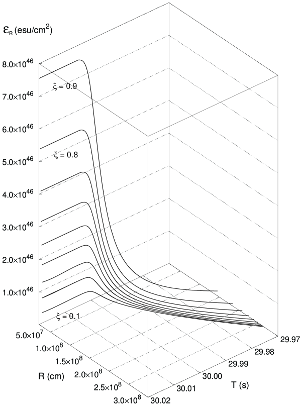
7.8 The maximum energy extractable from a black hole
The theoretical analysis of the collapsing shell considered in the previous section allows to reach a deeper understanding of the mass formula of black holes at least in the case of a Reissner–Nordström black hole. This allows as well to give an expression of the irreducible mass of the black hole only in terms of its kinetic energy of the initial rest mass undergoing gravitational collapse and its gravitational energy and kinetic energy at the crossing of the black hole horizon. It also allows to create a scenario for acceleration of the ultrahigh energy cosmic rays with energy typically eV from black holes, as opposed to the process of vacuum polarization producing pairs with energies in the MeV region. We shall follow in this Section the treatment by Ruffini and Vitagliano [407].
7.8.1 The formula of the irreducible mass of a black hole
The main objective of this section is to clarify the interpretation of the mass-energy formula [379] for a black hole. For simplicity we study the case of a nonrotating black hole using the results presented in the previous section. As we saw there, the collapse of a nonrotating charged shell can be described by exact analytic solutions of the Einstein–Maxwell equations. Consider to two complementary regions in which the world surface of the shell divides the space-time: and . They are static space-times; we denote their time-like Killing vectors by and respectively. is foliated by the family of space-like hypersurfaces of constant .
The splitting of the space-time into the regions and allows two physically equivalent descriptions of the collapse and the use of one or the other depends on the question one is studying. The use of proves helpful for the identification of the physical constituents of the irreducible mass while is needed to describe the energy extraction process from black hole. The equation of motion for the shell, Eq. 480, reduces in this case to
| (493) |
in and
| (494) |
in . The constraint (482) becomes
| (495) |
Since is a flat space-time we can interpret in (493) as the gravitational binding energy of the system. is its electromagnetic energy. Then Eqs. (493), (494) differ by the gravitational and electromagnetic self-energy terms from the corresponding equations of motion of a test particle.
Introducing the total radial momentum of the shell, we can express the kinetic energy of the shell as measured by static observers in as . Then from Eq. (493) we have
| (496) |
where we choose the positive root solution due to the constraint (495). Eq. (496) is the mass formula of the shell, which depends on the time-dependent radial coordinate and kinetic energy . If , a black hole is formed and we have
| (497) |
where and is the radius of the external horizon of that
| (498) |
so it follows that
| (499) |
namely that is the sum of only three contributions: the rest mass , the gravitational potential energy and the kinetic energy of the rest mass evaluated at the horizon. is independent of the electromagnetic energy, a fact noticed by Bekenstein [419]. We have taken one further step here by identifying the independent physical contributions to . This has important consequences for the energetics of black hole formation (see [406]).
Next we consider the physical interpretation of the electromagnetic term , which can be obtained by evaluating the Killing integral
| (500) |
where is the space-like hypersurface in described by the equation , with as its surface element vector. The quantity in Eq. (500) differs from the purely electromagnetic energy
| (501) |
where is the unit normal to the integration hypersurface and . This is similar to the analogous situation for the total energy of a static spherical star of energy density within a radius , , which differs from the pure matter energy
by the gravitational energy (see [393]). Therefore the term in the mass formula (496) is the total energy of the electromagnetic field and includes its own gravitational binding energy. This energy is stored throughout the region , extending from to infinity.
7.8.2 Extracting electromagnetic energy from a subcritical and overcritical black hole
We now turn to the problem of extracting the electromagnetic energy from a black hole (see [379]). We can distinguish between two conceptually physically different processes, depending on whether the electric field strength is smaller or greater than the critical value . The maximum value of the electric field around a black hole is reached at the horizon. In what follows we restore , and .
For the leading energy extraction mechanism consists of a sequence of discrete elementary decay processes of a particle into two oppositely charged particles. The condition implies
| (502) |
where is the Compton wavelength of the electron. Denardo and Ruffini [376] and Denardo, Hively and Ruffini [377] have defined as the effective ergosphere the region around a black hole where the energy extraction processes occur. This region extends from the horizon up to a radius
| (503) |
The energy extraction occurs in a finite number of such discrete elementary processes, each one corresponding to a decrease of the black hole charge. We have
| (504) |
Since the total extracted energy is (see Eq. (498)) , we obtain for the mean energy per accelerated particle
| (505) |
which gives
| (506) |
One of the crucial aspects of the energy extraction process from a black hole is its back reaction on the irreducible mass expressed in [379]. Although the energy extraction processes can occur in the entire effective ergosphere defined by Eq. (503), only the limiting processes occurring on the horizon with zero kinetic energy can reach the maximum efficiency while approaching the condition of total reversibility (see Fig. 2 in [379] for details). The farther from the horizon that a decay occurs, the more it increases the irreducible mass and loses efficiency. Only in the complete reversibility limit [379] can the energy extraction process from an extreme black hole reach the upper value of of the total black hole energy.
For the leading extraction process is the collective process based on the generation of the optically thick electron–positron plasma by the vacuum polarization. The condition implies
| (507) |
This vacuum polarization process can occur only for a black hole with mass smaller than . The electron–positron pairs are now produced in the dyadosphere of the black hole. We have
| (508) |
The number of particles created [398] is then
| (509) |
The total energy stored in the dyadosphere is [398]
| (510) |
The mean energy per particle produced in the dyadosphere is then
| (511) |
which can be also rewritten as
| (512) |
We stress again that the vacuum polarization around a black hole has been observed to reach theoretically the maximum efficiency limit of of the total mass-energy of an extreme black hole (see e.g. [398]).
Let us now compare and contrast these two processes. We have
| (513) |
Moreover we see (Eqs. (506), (512)) that is in the range of energies of UHECR (see [420] and references therein), while for and , is in the -ray range. In other words, the discrete particle decay process involves a small number of particles with ultrahigh energies (), while vacuum polarization involves a much larger number of particles with lower mean energies ().
7.9 A theorem on a possible disagreement between black holes and thermodynamics
This analysis of vacuum polarization process around black holes is so general that it allows as well to look back to traditional results on black hole physics with an alternative point of view. We quote in particular a result which allows to overcome a claimed inconsistency between general relativity and thermodynamics in the field of black holes.
It is well known that if a spherically symmetric mass distribution without any electromagnetic structure undergoes free gravitational collapse, its total mass-energy is conserved according to the Birkhoff theorem: the increase in the kinetic energy of implosion is balanced by the increase in the gravitational energy of the system. If one considers the possibility that part of the kinetic energy of implosion is extracted then the situation is very different: configurations of smaller mass-energy and greater density can be attained without violating Birkhoff theorem in view of the radiation process.
From a theoretical physics point of view it is still an open question how far such a sequence can go: using causality nonviolating interactions, can one find a sequence of braking and energy extraction processes by which the density and the gravitational binding energy can increase indefinitely and the mass-energy of the collapsed object be reduced at will? This question can also be formulated in the mass formula language [379] (see also Ref. [406]): given a collapsing core of nucleons with a given rest mass-energy , what is the minimum irreducible mass of the black hole which is formed?
Following the previous two sections, consider a spherical shell of rest mass collapsing in a flat space-time. In the neutral case the irreducible mass of the final black hole satisfies Eq. 499. The minimum irreducible mass is obtained when the kinetic energy at the horizon is , that is when the entire kinetic energy has been extracted. We then obtain, form Eq. 499, the simple result
| (514) |
We conclude that in the gravitational collapse of a spherical shell of rest mass at rest at infinity (initial energy ), an energy up to of can in principle be extracted, by braking processes of the kinetic energy. In this limiting case the shell crosses the horizon with . The limit in the extractable kinetic energy can further increase if the collapsing shell is endowed with kinetic energy at infinity, since all that kinetic energy is in principle extractable.
We have represented in Fig. 27 the world lines of spherical shells of the same rest mass , starting their gravitational collapse at rest at selected radii . These initial conditions can be implemented by performing suitable braking of the collapsing shell and concurrent kinetic energy extraction processes at progressively smaller radii (see also Fig. 28). The reason for the existence of the minimum (514) in the black hole mass is the “self-closure” occurring by the formation of a horizon in the initial configuration (thick line in Fig. 27).

Is the limit actually attainable without violating causality? Let us consider a collapsing shell with charge . If a black hole is formed. As pointed out in the previous section the irreducible mass of the final black hole does not depend on the charge . Therefore Eqs. (499) and (514) still hold in the charged case. In Fig. 28 we consider the special case in which the shell is initially at rest at infinity, i.e. has initial energy , for three different values of the charge . We plot the initial energy , the energy of the system when all the kinetic energy of implosion has been extracted as well as the sum of the rest mass energy and the gravitational binding energy of the system (here is the radius of the shell). In the extreme case , the shell is in equilibrium at all radii (see Ref. [405]) and the kinetic energy is identically zero. In all three cases, the sum of the extractable kinetic energy and the electromagnetic energy reaches of the rest mass energy at the horizon, according to Eq. (514).

What is the role of the electromagnetic field here? If we consider the case of a charged shell with , the electromagnetic repulsion implements the braking process and the extractable energy is entirely stored in the electromagnetic field surrounding the black hole (see Ref. [406]). We emphasize here that the extraction of of the mass-energy of a black hole is not specifically linked to the electromagnetic field but depends on three factors: a) the increase of the gravitational energy during the collapse, b) the formation of a horizon, c) the reduction of the kinetic energy of implosion. Such conditions are naturally met during the formation of an extreme black hole with , but as we have seen, they are more general and can indeed occur in a variety of different situations, e.g. during the formation of a Schwarzschild black hole by a suitable extraction of the kinetic energy of implosion (see Fig. 27 and Fig. 28).
Before closing let us consider a test particle of mass in the gravitational field of an already formed Schwarzschild black hole of mass and go through such a sequence of braking and energy extraction processes. Kaplan [421] found for the energy of the particle as a function of the radius
| (515) |
It would appear from this formula that the entire energy of a particle could be extracted in the limit . Such efficiency of energy extraction has often been quoted as evidence for incompatibility between General Relativity and the second principle of Thermodynamics (see Ref. [422] and references therein). J. Bekenstein and S. Hawking have gone as far as to consider General Relativity not to be a complete theory and to conclude that in order to avoid inconsistencies with thermodynamics, the theory should be implemented through a quantum description [422, 423, 424, 425]. Einstein himself often expressed the opposite point of view (see, e.g., Ref. [426] and references therein).
The analytic treatment presented in Section 7.7.2 can clarify this fundamental issue. It allows to express the energy increase of a black hole of mass through the accretion of a shell of mass starting its motion at rest at a radius in the following formula which generalizes Eq. (515):
| (516) |
where is clearly the mass-energy of the final black hole. This formula differs from the Kaplan formula (515) in three respects: (a) it takes into account the increase of the horizon area due to the accretion of the shell; (b) it shows the role of the gravitational self-energy of the imploding shell; (c) it expresses the combined effects of (a) and (b) in an exact closed formula.
The minimum value of is attained for the minimum value of the radius : the horizon of the final black hole. This corresponds to the maximum efficiency of the energy extraction. We have
| (517) |
or solving the quadratic equation and choosing the positive solution for physical reasons
| (518) |
The corresponding efficiency of energy extraction is
| (519) |
which is strictly smaller than 100% for any given . It is interesting that this analytic formula, in the limit , properly reproduces the result of equation (514), corresponding to an efficiency of . In the opposite limit we have
| (520) |
Only for , Eq. (519) corresponds to an efficiency of 100% and correctly represents the limiting reversible transformations. It seems that the difficulties of reconciling General Relativity and Thermodynamics are ascribable not to an incompleteness of General Relativity but to the use of the Kaplan formula in a regime in which it is not valid.
7.10 Astrophysical gravitational collapse and black holes
The time evolution of the gravitational collapse (occurring on characteristic gravitational timescale s) and the associated electrodynamical process are too complex for direct description. We addressed here a more confined problem: the vacuum polarization process around an already formed Kerr–Newman black hole. This is a well defined problem which deserves attention. It is theoretically expected to represent a physical state asymptotically reached in the process of gravitational collapse. Such an asymptotic configuration will be reached when all multipoles departing from the Kerr–Newman geometry have been radiated away either by process of vacuum polarization or electromagnetic and gravitational waves. What is most important is that by performing this theoretical analysis we can have a direct evaluation of the energetics and of the spectra and dynamics of the plasma created on the extremely short timescale due to the quantum phenomena of s. This entire transient phenomena, starting from an initial neutral condition of the core in the progenitor star, undergoes the formation of the Kerr–Newman black hole by the collective effects of gravitation, strong, weak, electromagnetic interactions during a fraction of the above mentioned gravitational characteristic timescale of collapse.
After the process of vacuum polarization all the electromagnetic energy of incipient Kerr–Newman black hole will be radiated away and almost neutral Kerr solution will be left and reached asymptotically in time. In a realistic gravitational collapse the theoretical picture described above will be further amplified by the presence of high-energy processes including neutrino emission and gravitational waves emission with their electromagnetic coupling: the gravitationally induced electromagnetic radiation and electromagnetically induced gravitational radiation [427, 428].
Similarly, in the next Section we proceed to a deeper understanding of other collective plasma phenomena also studied in idealized theoretically well defined cases. They will play an essential role in the astrophysical description of the dynamical phase of gravitational collapse.
8 Plasma oscillations in electric fields
We have seen in the previous Sections the application of the Sauter-Heisenberg-Euler-Schwinger process for electron–positron pair production in the heavy nuclei, in the laser and in the last Section in the field of black holes. The case of black holes is drastically different from all the previous ones. The number of electron–positron pairs created is of the order of , the plasma expected is optically thick and is very different from the nuclear collisions and laser case where pairs are very few and therefore optically thin. The following dynamical aspects need to be addressed.
-
1.
the back reaction of pair production on the external electric field;
-
2.
the screening effect of pairs on the external electric field strengths;
-
3.
the motion of pairs and their interactions.
When these dynamical effects are considered, the pair production in an external electric field is no longer only a process of quantum tunneling in a constant static electric field. In fact, it turns out to be a much more complex process during which all the three above mentioned effects play an important role. More precisely, a phenomenon of electron–positron oscillation, plasma oscillation, takes place. We are going to discuss such plasma oscillation phenomenon in this Section. As we will see in this Section these phenomena can become also relevant for heavy-ion collisions. After giving the basic equations for description of plasma oscillations we give first some applications in the field of heavy ions. In this Section in all formulas we use .
8.1 Semiclassical theory of plasma oscillations in electric fields
In the semi-classical QED [429, 430], one quantizes only the Dirac field , while an external electromagnetic field is treated classically as a mean field. This is the self-consistent mean field or Gaussian approximation that can be formally derived as the leading term in the large- limit of QED, where is the number of charged matter fields [430, 431, 432, 433, 434]. The motion of these electrons can be described by a Dirac equation in an external classical electromagnetic potential
| (521) |
and the semi-classical Maxwell equation
| (522) |
where is the electron and positron current and the expectation value is with respect to the quantum states of the electron field. The dynamics that these equations describe is not only the motion of electron and positron pairs, but also their back reaction on the external electromagnetic field. The resultant phenomenon is the so-called plasma oscillation that we will discuss based on both a simplified model of semi-classical scalar QED and kinetic Boltzmann-Vlasov equation as presented in Refs. [429, 430, 435, 436, 437].
A scheme for solving the back reaction problem in scalar QED was offered in Refs. [429, 430]. Based on this scheme, a numerical analysis was made in (1+1)-dimensional case [435]. Eqs. (521), (522) are replaced by the scalar QED coupled equations for a charged scalar field
| (523) |
The current of the charged scalar field in the semi-classical Maxwell equations (522) is
| (524) |
Now, consider a spatially homogeneous electric field in the -direction. A corresponding gauge potential is . Defining , and , the Maxwell equations (522) reduce to the single equation
| (525) |
for the potential and .
The quantized scalar field in Eq. (523) can be expanded in terms of plane waves with operator-valued amplitudes and
| (526) |
where is the volume of the system and the time-independent creation and annihilation operators obey the commutation relations
| (527) |
and each -mode function obeys the Wronskian condition,
| (528) |
The time dependency in this basis (526,527) is carried by the complex mode functions that satisfy the following equation of motion, as demanded from the QED coupled Eq. (523) of Klein–Gordon type
| (529) |
where the time-dependent frequency is given by
| (530) |
Here is the constant canonical momentum in the -direction which should be distinguished from the gauge invariant, but time-dependent kinetic momentum
| (531) |
which reflects the acceleration of the charged particles due to the electric field, while in the directions transverse to the electric field the kinetic and canonical momenta are the same .
The mean value of electromagnetic current (524) in the -direction is then
| (532) |
where and are the mean numbers of particles and antiparticles in the time-independent basis (526,527). The mean charge density must vanish
by the Gauss law for a spatially homogeneous electric field (i.e., ). As a result, . For the vacuum state, . The Maxwell equation (525) for the evolution of electric field becomes
| (533) |
These two scalar QED coupled Eqs. (529) and (533) in (1+1)-dimensional case were numerically integrated in Ref. [435]. The results are shown in Fig. 29, where the time evolutions of the scaled electric field and current are shown as functions of time in unit of Compton time . Starting with a strong electric field, one clearly finds the phenomenon of oscillating electric field and current , i.e., plasma oscillation.

This phenomenon of plasma oscillation is shown in Fig. 29 and is easy to understand as follows. In a classical kinetic picture, we have the electric current where is the density of electrons (or positrons) and is their mean velocity. Driven by the external electric field, the velocity of electrons (or positrons) continuously increases, until the electric field of electron and positron pairs screens the external electric field down to zero, and the kinetic energy of electrons (or positrons) reaches its maximum. The electric current saturates as the velocity is close to the speed of light. Afterward, these electrons and positrons continuously move apart from each other further, their electric field, whose direction is opposite to the direction of the external electric field, increases and decelerates electrons and positrons themselves. Thus the velocity of electrons and positrons decreases, until the electric field reaches negative maximum and the velocity vanishes. Then the velocity of electrons and positrons starts to increase in backward direction and the electric field starts to decrease for another oscillation cycle.
8.2 Kinetic theory of plasma oscillations in electric fields
In describing the same system as in the previous section it can be used, alternatively to the semi-classical theory, a phenomenological model based on the following relativistic Boltzmann-Vlasov equation [435]
| (534) |
where the -independent function is a classical distribution function of particle and antiparticle pairs in phase space. The source term in the right-hand side of Eq. (534) is related to the Schwinger rate (161) for the pair production of spin- particle and antiparticle
| (535) |
where the -function expresses the fact that particles are produced at rest and the factor accounts for stimulated pair production (Bose enhancement). The Boltzmann-Vlasov equation (534) for the distribution function is in fact attributed to the conservation of particle number in phase space.
In the field equation (525) for the classical gauge potential , the electric current is contributed from the conduction current
| (536) |
and the polarization current [438]
| (537) |
The relativistic Boltzmann-Vlasov equation (534) and field equation (525) with the conduction current (536) and the polarization current (537) were numerically integrated [435] in (1+1)-dimensional case. The numerical integration shows that the system undergoes plasma oscillations. In Fig. 29 the results of the semi-classical analysis and the numerical integration of the Boltzmann equation are compared. We see that they are in good quantitative agreement. The discrepancies are because in addition to spontaneous pair production, the quantum theory takes into account pair production via bremsstrahlung (“induced” pair production), which are neglected in Eq. (534)).
In Refs. [439, 440], the study of plasma oscillation was extended to the fermionic case. On the basis of semi-classical theory of spinor QED, expressing the solution of the Dirac equation (521) as
where is a four-component spinor, one finds that satisfies the quadratic Dirac equation,
| (538) |
The electric current of spinor field couples to the external electric field that obeys the field equation (525).
The source term in the right-hand side of the kinetic Boltzmann-Vlasov equation (534) is changed to the Schwinger rate (160) for the pair production of electrons and positrons,
| (539) |
where the Pauli blocking is taken into account by the factor . Analogously to the scalar QED case, both semi-classical theory of spinor QED and kinetic Boltzmann-Vlasov equation have been analyzed and numerical integration was made in the (1+1)-dimensional case [439, 440]. The numerical results show that plasma oscillations of electric field, electron and positron currents are similar to that plotted in Fig. 29.
8.3 Plasma oscillations in the color electric field of heavy ions
The Relativistic Heavy-Ion Collider (RIHC) at Brookhaven National Laboratory and Large Hadron Collider (LHC) at CERN are designed with the goal of producing a phase of deconfined hadronic matter: the quark-gluon plasma. A popular theoretical model for studying high-energy heavy-ion collisions begins with the creation of a flux tube containing a strong color electric field [441]. The field energy is converted into particles such as quark and antiquark pairs and gluons that are created by the Sauter–Euler–Heisenberg–Schwinger quantum tunneling mechanism. A relativistic Boltzmann–Vlasov equation coupling to such particle creation source is phenomenologically adopted in a kinetic theory model for the hydrodynamics of quark and gluon plasma [438, 442, 443, 444, 445, 446, 447].
In the collision of heavy-ion beams, one is clearly dealing with a situation that is not spatially homogeneous. However, particle production in the central rapidity region can be modeled as hydrodynamical system with longitudinal boost invariance [448, 449, 450, 451, 452]. To express the longitudinal boost invariance of the hydrodynamical system, one introduces the comoving coordinates: fluid proper time and rapidity by the relationships [453]
| (540) |
in terms of the Minkowski time and the coordinate along the beam direction in the ordinary laboratory frame. The line element and metric tensor in these coordinates are given by
| (541) |
and
where the vierbein transforms the curvilinear coordinates to Minkowski coordinates and . The covariant derivative on fermion field is given by [454]
| (542) |
and the spin connection is
with the usual Christoffel symbols and the usual coordinate-independent Dirac gamma matrices. The coordinate-dependent gamma matrices are obtained via
In the curved space time (541), the Dirac equation (521) and semi-classical Maxwell equation (522) are modified as
| (543) |
and
| (544) |
The phenomenological Boltzmann–Vlasov equation in (3+1)-dimensions can be also written covariantly as
| (545) |
where is the total proper time derivative. This kinetic transport equation is written in the comoving coordinates and their conjugate momenta:
Due to the longitudinal boost invariance, energy density and color electric field are spatially homogeneous, i.e., they are functions of the proper time only [453]. Consequently, the approach for spatially homogeneous electric field presented in Refs. [430, 435, 439, 440] and discussed in the previous Section 8.2 is applicable to the phenomenon of plasma oscillations in ultrarelativistic heavy-ion collisions [453] using Eq. 543 (resp. Eq. 545) in the place of Eq. 521 (resp. Eq. 534).
8.4 Quantum Vlasov equation
To understand the connection between the two frameworks of semi-classical field theory and classical kinetic theory, both of which describe the plasma oscillations, one can try to study a quantum transport equation in the semi-classical theory [437, 455, 456, 457]. For this purpose, a Bogoliubov transformation from the time-independent number basis () (526, 527) to a time-dependent number basis [] is introduced [437, 455, 456],
| (546) | |||||
| (547) |
and
| (548) | |||||
| (549) |
where and are the Bogoliubov coefficients. They obey
for each mode k. In the limit of very slowly varying as a function of time (530), i.e., and , the adiabatic number basis [] is defined by first constructing the adiabatic mode functions,
| (550) |
The particle number in the time-dependent adiabatic number basis is given by
| (551) | |||||
which though time-dependent, is an adiabatic invariant of the motion. Consequently, it is a natural candidate for a particle number density distribution function in the phase space, that is needed in a kinetic description.
By differentiating (551) and using the basic relationships (530,547,550), one obtains,
| (552) |
and
| (553) |
These two equations give rise to the quantum Vlasov equations [437, 455, 456],
| (554) | |||||
| (555) |
describing the time evolution of the adiabatic particle number of the mean field theory. describes the quantum creation rate of particle number in an arbitrary slowly varying mean field. The Bose enhancement and Pauli blocking factors appear in Eq. (555) so that both spontaneous and induced particle creation are included automatically in the quantum treatment. The most important feature of Eq. (555) is that the source term is nonlocal in time, indicating the particle creation rate depending on the entire history of the system. This means that the time evolution of the particle number governed by the quantum Vlasov equation is a non-Markovian process.
The mean electric current (532) in the basis of adiabatic number (547,549) can be rewritten as,
| (556) | |||||
| (557) | |||||
| (558) |
by using Eqs. (551), (552). This means electric current enters into the right-hand side of the field equation (525).
For the comparison between the quantum Vlasov equation (555) and the classical Boltzmann–Vlasov equation (534), the adiabatic particle number has to be understood as the counterpart of the classical distribution function of particle number in the phase space. The source term, that is composed by the Schwinger rate of pair production and the factor for either the Bose enhancement or Pauli blocking, is phenomenologically added into in the Boltzmann–Vlasov equation (534). Such source term is local in time, indicating that the time evolution of the classical distribution function is a Markovian process. In the limit of a very slowly varying uniform electric field and at very large time the source term (555) integrated over momenta reduces to the source term in the Boltzmann–Vlasov equation (534) [437, 455, 456]. As a result, the conduction current and the polarization current in Eq. (556) are reduced to their counterparts Eqs. (536), (537) in the phenomenological model of kinetic theory. In Ref. [437, 458, 459, 460, 267], the quantum Vlasov equation has been numerically studied to show the plasma oscillations and the non-Markovian effects. They are also compared with the Boltzmann–Vlasov equation (534) that corresponds to the Markovian limit.
8.5 Quantum decoherence in plasma oscillations
As showed in Fig. 29, the collective oscillations of electric field and associate electric current are damped in their amplitude. Moreover, as time increases, a decoherence in their oscillating frequency occurs [435, 461]. This indicates that plasma oscillations decay in time. This effective energy dissipation or time irreversibility is the phenomenon of quantum decoherence [462] in the process of creation and oscillation of particles, in the sense that energy flows from collective motion of the classical electromagnetic field to the quantum fluctuations of charged matter fields without returning back over times of physical interest [461, 463]. This means that the characteristic frequency of the quantum fluctuation mode “” is much larger than the frequency of the classical electric field: and [437, 461], where is the number density of particles and antiparticles. The study of quantum decoherence and energy dissipation associated with particle production to understand the plasma oscillation frequency and damping can be found in Refs. [437, 461, 463].
To understand the energy dissipation from the collective oscillation of classical mean fields to rapid fluctuations of quantum fields, it is necessary to use the Hamiltonian formalism of semi-classical theory. One defines the quantum fluctuation upon classical mean field in the semi-classical scalar theory [437, 461, 463],
| (559) |
where is the Fourier component of the quantized scalar field (526). In the time-independent basis (527,528), one has (see Section 8),
| (560) |
and the mode equation (529) for can be rewritten as
| (561) |
where is the momentum canonically conjugate to . Moreover, the semi-classical Maxwell equation (533) is rewritten as
| (562) |
Eqs. (561) and (562) actually are Hamilton equations of motion,
| (563) |
for a closed system with Hamiltonian,
| (564) |
where is the momentum canonically conjugate to , is the field-dependent frequency of quantum fluctuations given by Eq. (530) and the value of mean field (559) vanishes, , for each -mode. In Eq. (564), the first term is the electric energy and the second term is the energy of quantum fluctuations of charged matter field, interacting with electric field.
Quantum decoherence can be studied within this Hamiltonian framework. If one considers only the time evolution of classical electric field , that is influenced by the quantum fluctuating modes , the latter can be treated as a heat bath “environment”. Quantitative information about the quantum decoherence is contained in the so-called influence functional, which is a functional of two time evolution trajectories and [461]
| (565) |
where are different time evolution states determined by Eq. (563), starting with the same initial state and initial vacuum condition (533). One finds [461]
| (566) |
in terms of the two sets of mode functions and (the subscript is omitted). This (566) is precisely the closed time path (CTP) effective action functional which generates the connected real -points vertices in the quantum theory [464, 465, 466, 467, 468, 469, 470, 471]. The absolute value of (565) measures the influence of quantum fluctuations on the time evolution of the classical electric field , i.e., the effect of quantum decoherence. If there is no influence of quantum fluctuations on , then and , otherwise deviates from , and . Numerical results about the damping and the decoherence of the electric field are presented in Refs. [435, 461] (see Figs. 29 and 30).
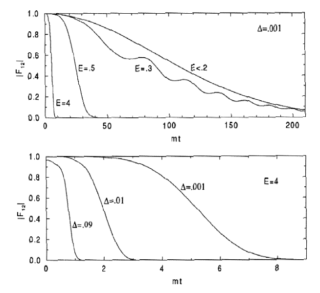
The effective damping discussed above is certainly collisionless, since the charged particle modes interact only with the electric field but not directly with each other. The damping of plasma oscillation attributed to the collisions between charged particle modes will be discussed in the next section.
8.6 Collision decoherence in plasma oscillations
If there are interactions between different modes and species of particles, the time evolutions of electric field and the distribution function of particle number in the phase space are certainly changed. This can be phenomenologically studied in the relativistic Boltzmann-Vlasov equation (534) by adding collision terms ,
| (567) |
These collision terms describe not only the interactions of different modes of particles, but also interactions of different species of particles, for example, electron and positron annihilation to two photons and vice versa. In Refs. [458, 460], the following equilibrating collision terms were considered,
| (568) |
where is the thermal (Fermi or Bose) distribution function of particle number (fermions or bosons) at temperature , the relaxation time is determined by the mean free path and mean velocity of particles, through
| (569) |
and is a dimensionless parameter. is computed from the number density of particles,
| (570) |
Whereas, the mean velocity of particles is given by , expressed in terms of mean kinetic momentum and energy of particles. The mean values of momentum and energy are computed [460] by using distribution function regularized via the procedure described in Ref. [458] that yields the renormalized electric current (556). The temperature in Eq. (568) is the “instantaneous temperature”, which is determined by requiring that at each time the mean particle energy is identical to that in an equilibrium distribution at the temperature ,
| (571) |
This system of two coupled equations: (i) the field equation (525) with renormalized electric currents (556); (ii) the relativistic Boltzmann-Vlasov equation (567) with the source term (555) and equilibrating collision term (568), are numerically integrated in Refs. [458, 460]. One of these numerical results is presented in Fig. 31. It shows [458] that when the collision timescale (569) is much larger than the plasma oscillation timescale , , the plasma oscillations are unaffected. On the other hand, when the collision term has a significant impact on both the amplitude and the frequency of the oscillations that result damped. There is a value of below which no oscillations arise and the system evolves quickly and directly to thermal equilibrium. It is worthwhile to contrast this collision damping of plasma oscillation with the collisionless damping effect due to rapid quantum fluctuations described in Section 8.5.
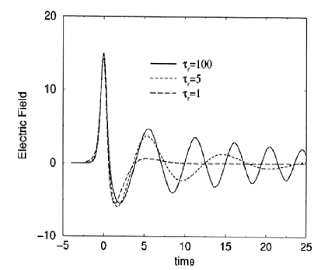
8.7 interactions in plasma oscillations in electric fields
In this section, a detailed report of the studies [72] of the relativistic Boltzmann-Vlasov equations for electrons, positrons and photons with collision terms originated from annihilation of electrons and positrons pair into two photons and vice versa is presented. These collision terms lead to the damping of plasma oscillation and possibly to energy equipartition between different types of particles.We focus on the evolution of a system of pairs created in a strongly overcritical electric field (), explicitly taking into account the process . Since it is far from equilibrium the collisions cannot be modeled by an effective relaxation time term in the transport equations, as discussed in the previous section. Rather the actual, time varying, collision integrals have to be used.
Furthermore we are mainly interested in a system in which the electric field varies on macroscopic length scale and therefore one can approximate an electric field as a homogeneous one. Also, transport equations are used for electrons, positrons and photons, with collision terms, coupled to Maxwell equations, as introduced in Section 8.1 and 8.2. There is no free parameter here: the collision terms can be exactly computed, since the QED cross-sections are known. Starting from a regime which is far from thermal equilibrium, one finds that collisions do not prevent plasma oscillations in the initial phase of the evolution and analyze the issue of the timescale of the approach to an plasma equilibrium configuration.
As discussed in Section 8.1 and 8.2 one can describe positrons (electrons) created by vacuum polarization in a strong homogeneous electric field through the distribution function () in the phase space of positrons (electrons). Because of homogeneity () only depend on the time and the positron (electron) 3–momentum :
| (572) |
Moreover, because of particle–antiparticle symmetry, one also has
| (573) |
Analogously photons created by pair annihilation are described through the distribution function in the phase space of photons. is the photon 3–momentum , then
| (574) |
and are normalized so that
| (575) | ||||
| (576) |
where and are number densities of positrons (electrons) and photons, respectively. For any function of the momenta, one can denote by
| (577) |
or
| (578) |
its mean value in the phase space of positrons (electrons) or photons, respectively.
The motion of positrons (electrons) is the result of three contributions: the pair creation, the electric acceleration and the annihilation damping. The probability density rate for the creation of a pair with 3–momentum in the electric field is given by the Schwinger formula (see also Refs. [435, 439]):
| (579) |
where and are the components of the 3-momentum parallel and orthogonal to , respectively. Also the energy is introduced
| (580) |
of an electron of 3-momentum and the energy
| (581) |
of a photon of 3-momentum . Then, the probability density rate for the creation (destruction) of a fermion with 3-momentum is given by
| (582) |
where
| (583) |
is the matrix element for the process
| (584) |
and as a first approximation, Pauli blocking and Bose enhancement (see, for instance, Ref. [439]) are neglected. Analogously the probability density rate for the creation (annihilation) of a photon with 3-momentum is given by
| (585) |
Finally the evolution of the pairs is governed by the transport Boltzmann–Vlasov equations
| (586) | ||||
| (587) |
Note that the collisional terms (582) and (585) are negligible, when created pairs do not produce a dense plasma.
Because pair creation back reacts on the electric field, as seen in Section 8.1 and 8.2, Vlasov equations are coupled with the homogeneous Maxwell equations, which read
| (588) |
where
| (589) |
is the polarization current and
| (590) |
is the conduction current (see Ref. [438]).
Eqs. (586), (587) and (588) describe the dynamical evolution of the electron–positron pairs, the photons and the strong homogeneous electric field due to the Schwinger process of pair creation, the pair annihilation into photons and the two photons annihilation into pairs. It is hard to (even numerically) solve this system of integral and partial differential equations. It is therefore useful to introduce a simplification procedure of such a system through an approximation scheme. First of all note that Eqs. (586) and (587) can be suitably integrated over the phase spaces of positrons (electrons) and photons to get differential equations for mean values. The following exact equations for mean values are obtained:
| (591) |
where
| (592) | ||||
| (593) |
is the total probability rate for Schwinger pair production. In Eqs. (591), the velocity of light and is the relative velocity between electrons and positrons in the reference frame of the center of mass, where , are 3–momenta of electron and positron and are their energies. is the total cross-section for the process , and is the total cross-section for the process , here is the energy of a particle in the reference frame of the center of mass.
In order to evaluate the mean values in system (591) some further hypotheses on the distribution functions are needed. One defines , and such that
| (594) |
| (595) |
It is assumed
| (596) |
Since in the scattering the coincidence of the scattering direction with the incidence direction is statistically favored, it is also assumed
| (597) |
where and have analogous meaning as and and the terms and account for the probability of producing, respectively, forwardly scattered and backwardly scattered photons. Since the Schwinger source term (579) implies that the positrons (electrons) have initially fixed , namely , assumption (596) ((597)) means that the distribution of () does not spread too much with time and, analogously, that the distribution of energies is sufficiently peaked to be describable by a –function. As long as this condition is fulfilled, approximations (596) and (597) are applicable. The actual dependence on the momentum of the distribution functions has been discussed in Ref. [439, 437]. If Eqs. (596) and (597) are substituted into the system (591) one gets a new system of ordinary differential equations. One can introduce the inertial reference frame which on average coincides with the center of mass frame for the processes , and has for each species, and therefore substituting Eqs. (596) and (597) into Eqs. (591) one finds
| (598) |
where
| (599) | ||||
| (600) | ||||
| (601) |
are the energy density of positrons (electrons), the energy density of photons and the density of “parallel momentum” of positrons (electrons), is the electric field strength and the unique component of parallel to . and are evaluated at for each species. Note that Eqs. (598) are “classical” in the sense that the only quantum information is encoded in the terms describing pair creation and scattering probabilities. Finally Eqs. (598) are duly consistent with energy density conservation:
| (602) |
Eqs. (598) have to be integrated with the following initial conditions
In Fig. 32 the results of the numerical integration for is showed. The integration stops at (where, as usual, is the Compton time of the electron). Each quantity is represented in units of and , the Compton length of the electron.

-
1.
the electric field does not abruptly reach the equilibrium value but rather oscillates with decreasing amplitude;
-
2.
electrons and positrons oscillates in the electric field direction, reaching ultrarelativistic velocities;
-
3.
the role of the scatterings is marginal in the early time of the evolution.
This last point can be easily explained as follows: since the electrons are too extremely relativistic, the annihilation probability is very low and consequently the density of photons builds up very slowly (see details in Fig. 32).
At late times the system is expected to relax to an equilibrium configuration and assumptions (596) and (597) have to be generalized to take into account quantum spreading of the distribution functions. It is nevertheless instructive to look at the solutions of Eqs. (598) in this regime. Moreover, such a solution should give information at least at the order of magnitude level. In Fig. 33 the numerical solution of Eqs. (598) is plotted, but the integration extends here all the way up to (the timescale of oscillations is not resolved in these plots).

It is interesting that the leading term recovers the expected asymptotic behavior:
-
1.
the electric field is screened to about the critical value: for ;
-
2.
the initial electromagnetic energy density is distributed over electron–positron pairs and photons, indicating energy equipartition;
-
3.
photons and electron–positron pairs number densities are asymptotically comparable, indicating number equipartition.
At such late times a regime of thermalized electrons–positrons–photons plasma is expected to begin (as qualitatively indicated by points 2 and 3 above) during which the system is describable by hydrodynamic equations [408, 399].
Let us summarize the results in this section. A very simple formalism is provided to describe simultaneously the creation of electron–positron pairs by a strong electric field and the pairs annihilation into photons. As discussed in literature, one finds plasma oscillations. In particular the collisions do not prevent such a feature. This is because the momentum of electrons (positrons) is very high, therefore the cross-section for the process is small and the annihilation into photons is negligible in the very first phase of the evolution. As a result, the system takes some time () to reach an equilibrium plasma configuration.
8.8 Electro-fluidodynamics of the pair plasma
In the previous section, collisional terms in the Vlasov-Boltzmann equation are introduced, describing interaction of pairs and photons via the reaction . These results have been considered of interest in the studies of pair production in free electron lasers [60, 238, 239, 264, 261], in optical lasers [472], of millicharged fermions in extensions of the standard model of particle physics [473], electromagnetic wave propagation in a plasma [269], as well in astrophysics [408].
In this section, following [73, 474], the case of undercritical electric field is explored. It is usually expected that for back reaction of the created electrons and positrons on the external electric field can be neglected and electrons and positrons would move as test particles along lines of force of the electric field. Here it is shown that this is not the case in a uniform unbounded field. This work is important since the first observation of oscillations effects should be first detectable in experiments for the regime , in view of the rapid developments in experimental techniques, see e.g. [270, 273, 274].
An approach is introduced based on continuity, energy-momentum conservation and Maxwell equations in order to account for the back reaction of the created pairs. This approach is more simple than the one, presented in the previous section. However, the final equations coincide with (598) when the interaction with photons can be neglected. By this treatment one can analyze the new case of undercritical field, , and recover the old results for overcritical field, . In particular, the range is focused.
It is generally assumed that electrons and positrons are created at rest in pairs, due to vacuum polarization in uniform electric field with strength [20, 7, 25, 26, 27, 33, 203, 204], with the average rate per unit volume and per unit time (164)
| (603) |
This formula is derived for uniform constant in time electric field. However, it still can be used for slowly time varying electric field provided the inverse adiabaticity parameter [203, 204, 36, 30, 31, 32, 244], see Eq. (355), is much larger than one,
| (604) |
where is the frequency of oscillations, is dimensionless period of oscillations. Equation (604) implies that time variation of the electric field is much slower than the rate of pair production. In two specific cases considered in this section, and one finds for the first oscillation and respectively. This demonstrates applicability of the formula (603) in this case.
From the continuity, energy-momentum conservation and Maxwell equations written for electrons, positrons and electromagnetic field one can have
| (605) | ||||
| (606) | ||||
| (607) |
where is the comoving number density of electrons, is energy-momentum tensor of electrons and positrons
| (608) |
is electromagnetic field tensor, is the total 4-current density, is four velocity respectively of positrons and electrons
| (609) |
is the average velocity of electrons, is relativistic Lorentz factor. Electrons and positrons move along the electric field lines in opposite directions.
One can choose a coordinate frame where pairs are created at rest. Electric field in this frame is directed along -axis. In spatially homogeneous case from (605) one has for coordinate number density
| (610) |
With definitions (608) from (606) and equation of motion for positrons and electrons
| (611) |
one finds
| (612) |
where the total 4-current density is the sum of conducting and polarization currents [438] densities
| (613) | ||||
| (614) | ||||
| (615) |
Energy-momentum tensor in (606) and electromagnetic field tensor in (607) change for two reasons: 1) electrons and positrons acceleration in the electric field, given by the term , 2) particle creation, described by the term . Equation (605) is satisfied separately for electrons and positrons.
Defining energy density of positrons
| (616) |
one can find from (606)
| (617) |
Due to homogeneity of the electric field and plasma, electrons and positrons have the same energy and absolute value of the momentum density , but their momenta have opposite directions. The definitions also imply for velocity and momentum densities of electrons and positrons
| (618) |
and
| (619) |
which is just relativistic relation between the energy, momentum and mass densities of particles.
Gathering together the above equations one then has the following equations
| (620) | ||||
| (621) | ||||
| (622) | ||||
| (623) |
From (621) and (623) one obtains the energy conservation equation
| (624) |
where is the constant of integration, so the particle energy density vanishes for initial value of the electric field, .
These equations give also the maximum number of the pair density asymptotically attainable consistently with the above rate equation and energy conservation
| (625) |
For simplicity dimensionless variables , , , , and are introduced. With these variables the system of equations (620)-(623) takes the form
| (626) | ||||
where , and , as before.
The system of equations (626) is solved numerically with the initial conditions , and the electric field .
In fig. 34, electric field strength, number density, velocity and Lorentz gamma factor of electrons as functions of time, are presented for initial values of the electric field (left column) and (right column). Slowly decaying plasma oscillations develop in both cases. The half-life of oscillations to be for and for are estimated respectively. The period of the fist oscillation is and , the Lorentz factor of electrons and positrons in the first oscillation equals and respectively for and . Therefore, in contrast to the case , for plasma oscillations develop on a much longer timescale, electrons and positrons reach extremely relativistic velocities.

In fig. 35 the characteristic length of oscillations is shown together with the distance between the pairs at the moment of their creation. For constant electric field the formation length for the electron–positron pairs, or the quantum tunneling length, is not simply , as expected from a semi-classical approximation, but [28, 46]
| (627) |
Thus, given initial electric field strength one can define two characteristic distances: , the distance between created pairs, above which pair creation is possible, and the length of oscillations, , above which plasma oscillations occur in a uniform electric field. The length of oscillations is the maximal distance between two turning points in the motion of electrons and positrons (see fig. 35). From fig. 35 it is clear that . In the oscillation phenomena the larger electric field is, the larger becomes the density of pairs and therefore the back reaction, or the screening effect, is stronger. Thus the period of oscillations becomes shorter. Note that the frequency of oscillation is not equal to the plasma frequency, so it cannot be used as the measure of the latter. Notice that for the length of oscillations becomes macroscopically large.


At fig. 36 maximum Lorentz gamma factor in the first oscillation is presented depending on initial value of the electric field. Since in the successive oscillations the maximal value of the Lorentz factor is monotonically decreasing (see fig. 34) It is concluded that for every initial value of the electric field there exists a maximum Lorentz factor attainable by the electrons and positrons in the plasma. It is interesting to stress the dependence of the Lorentz factor on initial electric field strength. The kinetic energy contribution becomes overwhelming in the case. On the contrary, in the case the electromagnetic energy of the field goes mainly into the rest mass energy of the pairs.
This diagram clearly shows that never in this process the test particle approximation for the electrons and positrons motion in uniform electric field can be applied. Without considering back reaction on the initial field, electrons and positrons moving in a uniform electric field would experience constant acceleration reaching for on the timescale and keep that speed thereafter. Therefore, the back reaction effects in a uniform field are essential both in the case of and .
The average rate of pair creation is compared for two cases: when the electric field value is constant in time (an external energy source keeps the field unchanged) and when it is self-regulated by equations (626). The result is represented in fig. 37. It is clear from fig. 37 that when the back reaction effects are taken into account, the effective rate of the pair production is smaller than the corresponding rate (603) in a uniform field . At the same time, discharge of the field takes much longer time. In order to quantify this effect we need to compute the efficiency of the pair production defined as where is the time when pair creation with the constant rate would stop, and is defined above, see (625). For one finds %, while for one has %.
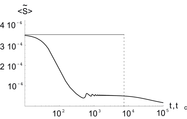
It is clear from the structure of the above equations that for the number of pairs is small, electrons and positrons are accelerated in electric field and the conducting current dominates. Assuming electric field to be weak, the polarization current is neglected in energy conservation (621) and in Maxwell equation (623). This means energy density change due to acceleration is much larger than the one due to pair creation,
| (628) |
In this case oscillations equations (620)-(623) simplify. From (621) and (622) one has , and using (618) obtains . This is the limit when rest mass energy is much smaller than the kinetic energy, .
One may therefore use only the first and the last equations from the above set. Taking time derivative of the Maxwell equation one arrives to a single second order differential equation
| (629) |
Equation (629) is integrated numerically to find the length of oscillations shown in fig. 35 for . Notice that condition (628) means ultrarelativistic approximation for electrons and positrons, so that although according to (620) there is creation of pairs with rest mass for each pair, the corresponding increase of plasma energy is neglected, as can be seen from (628).
Now one can turn to qualitative properties of the system (620)–(623). These nonlinear ordinary differential equations describe certain dynamical system which can be studied by using methods of qualitative analysis of dynamical systems. The presence of the two integrals (619) and (624) allows reduction of the system to two dimensions. It is useful to work with the variables and . In these variables one has
| (630) | ||||
| (631) |
Introducing the new time variable
| (632) |
one arrives at
| (633) | ||||
| (634) |
Clearly the phase space is bounded by the two curves . Moreover, physical requirement leads to existence of two other bounds . This system has only one singular point in the physical region, of the type focus at and .
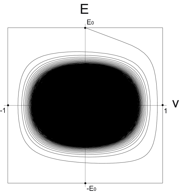
Thus, every phase trajectory tends asymptotically to the only singular point at and . This means oscillations stop only when electric field vanishes. At that point clearly
| (635) |
is valid. i.e. all the energy in the system transforms just to the rest mass of the pairs.
In order to illustrate details of the phase trajectories shown at fig. 38 only 1.5 cycles are plotted at fig. 39. One can see that the deviation from closed curves, representing undamped oscillations and shown by dashed curves, is maximal when the field peaks, namely when the pair production rate is maximal.
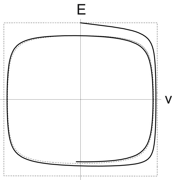
The above treatment has been done by considering uniquely back reaction of the electron–positron pairs on the external uniform electric field. The only source of damping of the oscillations is pair production, i.e. creation of mass. As analysis shows the damping in this case is exponentially weak. However, since electrons and positrons are strongly accelerated in electric field the bremsstrahlung radiation may give significant contribution to the damping of oscillations and further reduce the pair creation rate. Therefore, the effective rate shown in fig. 37 will represent an upper limit. In order to estimate the effect of bremsstrahlung, the classical formula for the radiation loss in electric field is recalled
| (636) |
Thus the equations (621) and (622), generalized for bremsstrahlung, are
| (637) | ||||
| (638) |
while equations (620) and (623) remain unchanged. Assuming that new terms are small, relations (619) and (624) are still approximately satisfied.
Now damping of the oscillations is caused by two terms:
| (639) |
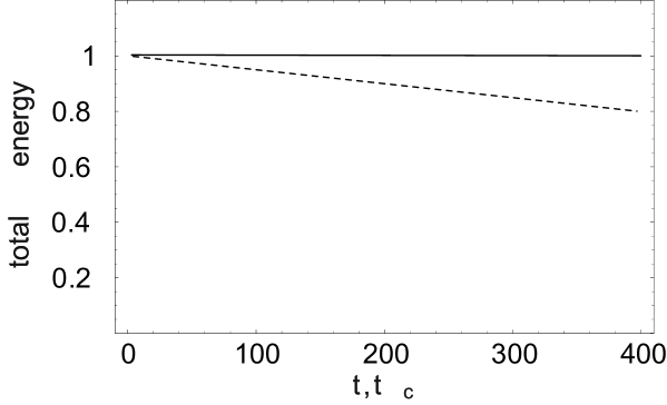
The modified system of equations is integrated, taking into account radiation loss, starting with . The results are presented in Fig. 40 where the sum of the energy of electric field and electron–positron pairs normalized to the initial energy is shown as a function of time. The energy loss reaches 20 percent for 400 Compton times. Thus the effect of bremsstrahlung is as important as the effect of collisions considered in [72] for , leading to comparable energy loss for pairs on the same timescale. For one expects that the damping due to bremsstrahlung dominates, but the correct description in this case requires Vlasov–Boltzmann treatment [74].
The damping of the plasma oscillations due to electron–positron annihilation into photons has been addressed in [72]. There it was found that the system evolves towards an electron–positron-photon plasma reaching energy equipartition. Such a system undergoes self-acceleration process following the work of [399].
Therefore the following conclusions are reached:
-
•
It is usually assumed that for electron–positron pairs, created by the vacuum polarization process, move as charged particles in external uniform electric field reaching arbitrary large Lorentz factors. The existence of plasma oscillations of the electron–positron pairs also for is demonstrated. The corresponding results for are well known in the literature. For both cases the maximum Lorentz factors reached by electrons and positrons are determined. The length of oscillations is 10 for , and 107 for . The asymptotic behavior in time, , of the plasma oscillations by the phase portrait technique is also studied.
-
•
For the vacuum polarization process transforms the electromagnetic energy of the field mainly in the rest mass of pairs, with moderate contribution to their kinetic energy: for one finds . For the kinetic energy contribution is maximized with respect to the rest mass of pairs: for .
-
•
In the case of oscillations the effective rate of pair production is smaller than the rate in uniform electric field constant in time, and consequently, the discharge process lasts longer. The half-life of oscillations is for and for . The efficiency of pair production is computed with respect to the one in a uniform constant field. For the efficiency is reduced to one percent, decreasing further for smaller initial electric field.
All these considerations apply to a uniform electric field unbounded in space. The presence of a boundary or a gradient in electric field would require the use of partial differential equations, in contrast to the ordinary differential equations used here. This topic needs further study. The effect of bremsstrahlung for is also estimated, and it is found that it represents comparable contribution to the damping of the plasma oscillations caused by collisions [72]. It is therefore clear, that the effect of oscillations introduces a new and firm upper limit to the rate of pair production which would be further reduced if one takes into account bremsstrahlung, collisions and boundary effects.
9 Thermalization of the mildly relativistic pair plasma
An electron–positron plasma is of interest in many fields of physics and astrophysics. In the early Universe [454, 475] during the lepton era, ultrarelativistic electron–positron pairs contributed to the matter contents of the Universe. In GRBs electron–positron pairs play an essential role in the dynamics of expansion [476, 477],[399]. Indications exist on the presence of the pair plasma also in active galactic nuclei [478], in the center of our Galaxy [479], around hypothetical quark stars [480]. In the laboratory pair plasma is expected to appear in the fields of ultraintense lasers [472].
In many stationary astrophysical sources the pair plasma is thought to be in thermodynamic equilibrium. A detailed study of the relevant processes [481, 482, 483, 484, 485, 486], radiation mechanisms [487], possible equilibrium configurations [483, 488] and spectra [489] in an optically thin pair plasma has been carried out. Particular attention has been given to collisional relaxation process [490, 491], pair production and annihilation [492], relativistic bremsstrahlung [493, 494], double Compton scattering [495, 496].
An equilibrium occurs if the sum of all reaction rates vanishes. For instance, electron–positron pairs are in equilibrium when the net pair production (annihilation) rate is zero. This can be achieved by variety of ways and the corresponding condition can be represented as a system of algebraic equations [497]. However, the main assumption made in all the above mentioned works is that the plasma is in thermodynamic equilibrium.
At the same time, in some cases considered above the pair plasma can be optically thick. Although moderately thick plasmas have been considered in the literature [498], only qualitative description is available for large optical depths. Assumption of thermal equilibrium is often adopted for rapidly evolving systems without explicit proof [476, 477],[399, 499]. Then hydrodynamic approximation is usually applied both for leptons and photons. However, particles may not be in equilibrium initially. Moreover, it is very likely situation, especially in the early Universe or in transient events when the energy is released on a very short timescale and there is not enough time for the system to relax to thermal equilibrium configuration.
Ultrarelativistic expansion of GRB sources is unprecedented in astrophysics. There are indications that relativistic jets in X-ray binaries have Lorentz factors while in active galactic nuclei [500], but some bursts sources have and possibly larger [501]. There is a consensus in the literature that the acceleration required to reach ultrarelativistic velocity in astrophysical flows comes from the radiation pressure, namely from photons and electron–positron pairs. Therefore, the source does not move as a whole, but expands from a compact region, almost reaching the speed of light. The bulk of radiation is emitted far from the region of formation of the plasma, when it becomes transparent for photons, trapped initially inside by the huge optical depth. Thus the plasma is optically thick at the moment of its formation and intense interactions between electrons, positrons and photons take place in it. Even if initially the energy is released in the form of only photons, or only pairs, the process of creation and annihilation of pairs soon redistribute the energy between particles in such a way that the final state will be a mixture of pairs and photons. The main question arises: what is the initial state, prior to expansion, of the pair plasma? Is it in a kind of equilibrium and, if so, is it thermal equilibrium, as expected from the optically thick plasma? Stationary sources in astrophysics have enough time for such an equilibrium to be achieved. On the contrary, for transient sources with the timescale of expansion of the order of milliseconds it is not at all clear that equilibrium can be reached.
In the literature there is no consensus on this point. Some authors considered thermal equilibrium as the initial state prior to expansion [476, 399], while others did not [77]. In fact, the study of the pair plasma equilibrium configurations in detail, performed in [488], cannot answer this question, because essentially nonequilibrium processes have to be considered.
Thus, observations provide motivation for theoretical analysis of physical conditions taking place in the sources of GRBs, and more generally, in nonequilibrium optically thick pair plasma. Notice that there is substantial difference between the ion-electron plasma on the one hand and electron–positron plasma on the other hand. Firstly, the former is collisionless in the wide range of parameters, while collisions are always essential in the latter. Secondly, when collisions are important relevant interactions in the former case are Coulomb scattering of particles which are usually described by the classical Rutherford cross-section. In contrast, interactions in the pair plasma are described by quantum cross-sections even if the plasma itself can be still considered as classical one.
The study reported in [74, 75] in the case of pure pair plasma clarified the issue of initial state of the pair plasma in GRB sources. The numerical calculations show that the pair plasma quickly reach thermal equilibrium prior to expansion, due to intense binary and triple collisions. In this Section details about the computational scheme adopted in [74] are given. Generalization to the presence of proton loading is given in [502].
9.1 Qualitative description of the pair plasma
First of all the domain of parameters characterizing the pair plasma considered in this Section is specified. It is convenient to use dimensionless parameters usually adopted for this purpose.
Mildly relativistic pair plasma is considered, thus the average energy per particle brackets the electron rest mass energy
| (640) |
The lower boundary is required for significant concentrations of pairs, while the upper boundary is set to avoid substantial production of other particles such as muons.
The plasma parameter is , where is the Debye length, is Boltzmann’s constant, and are electron number density and temperature respectively, is dimensionless temperature, is the plasma frequency. To ensure applicability of kinetic approach it is necessary that the plasma parameter is small, . This condition means that kinetic energy of particles dominates their potential energy due to mutual interaction. For the pair plasma considered in this Section this condition is satisfied.
Further, the classicality parameter, defined as , where is mean relative velocity of particles, see (753). The condition means that particles collisions can be considered classically, while for quantum description is required. Both for pairs and protons quantum cross-sections are used since .
The strength of screening of the Coulomb interactions is characterized by the Coulomb logarithm . Coulomb logarithm varies with mean particle velocity, and it cannot be set a constant as in most of studies of the pair plasma.
Finally, pair plasma is considered with linear dimensions exceeding the mean free path of photons , where is concentration of electrons and is the corresponding total cross-section. Thus the optical depth is large, and interactions between photons and other particles have to be taken in due account. These interaction are reviewed in the next section.
Note that natural parameter for perturbative expansion in the problem under consideration is the fine structure constant .
Pure pair plasma composed of electrons , positrons , and photons is considered. It is assumed that pairs or photons appear by some physical process in the region with a size and on a timescale . We assume that distribution functions of particles depend on neither spatial coordinates nor direction of momentum , i.e. isotropic in momentum space and uniform plasma is considered.
To make sure that classical kinetic description is adequate the dimensionless degeneracy temperature is estimated
| (641) |
and compared with the estimated temperature in thermal equilibrium. With initial conditions (640) the degeneracy temperature is always smaller than the temperature in thermal equilibrium and therefore the classical kinetic approach is applied. Besides, since ideal plasma is considered with the plasma parameter it is possible to use one-particle distribution functions. These considerations justify the computational approach based on classical relativistic Boltzmann equation. At the same time the right-hand side of Boltzmann equations contains collisional integrals with quantum and not classical matrix elements, as discussed above.
Relativistic Boltzmann equations [503],[504] in spherically symmetric case are
| (642) |
where , is the angle between the radius vector from the origin and the particle momentum , is a potential due to some external force, are particles velocities, are their distribution functions, the index denotes the type of particle, is their energy, and and are the emission and the absorption coefficients for the production of a particle of type “” via the physical process labeled by . This is a coupled system of partial–integro-differential equations. For homogeneous and isotropic distribution functions of electrons, positrons and photons Eqs. (642) reduce to
| (643) |
which is a coupled system of integro-differential equations. In (643) the Vlasov term is explicitly neglected.
Therefore, the left-hand side of the Boltzmann equation is reduced to partial derivative of the distribution function with respect to time. The right-hand side contains collisional integrals, representing interactions between electrons, positrons and photons.
Differential probability for all processes per unit time and unit volume [90] is defined as
| (644) |
where and are respectively momenta and energies of outgoing particles, are energies of particles before interaction, are the corresponding matrix elements, stands for energy-momentum conservation, is the normalization volume. The matrix elements are related to the scattering amplitudes by
| (645) |
As example consider absorption coefficient for Compton scattering which is given by
| (646) |
where and are momenta of electron (positron) and photon respectively, , and the differential probability is given by (691).
In (646) one can perform one integration over
| (647) |
but it is necessary to take into account the momentum conservation in the next integration over , so
| (648) | |||
where the Jacobian of the transformation is
| (649) |
where , , .
Finally, for the absorption coefficient
| (650) |
where the matrix element here is dimensionless. This integral is evaluated numerically.
For all binary interactions exact QED matrix elements are used which can be found in the standard textbooks, e.g. in [90],[322, 505], and are given below.
In order to account for charge screening in Coulomb scattering the minimal scattering angles are introduced following [506]. This allows to apply the same scheme for the computation of emission and absorption coefficients even for Coulomb scattering, while many treatments in the literature use Fokker-Planck approximation [507].
For such a dense plasma collisional integrals in (643) should include not only binary interactions, having order in Feynman diagrams, but also triple ones, having order [90]. Consider relativistic bremsstrahlung
| (651) |
For the time derivative, for instance, of the distribution function in the direct and in the inverse reactions (651) one has
| (652) | |||
where
and and are differential probabilities given by (644). The matrix element here has dimensions of the length squared.
In the case of the distribution functions (657), see below, there are multipliers proportional to in front of the integrals, where are chemical potentials. The calculation of emission and absorption coefficients is then reduced to the well known thermal equilibrium case [497]. In fact, since reaction rates of triple interactions are times smaller than binary reaction rates, it is expected that binary reactions come to detailed balance first. Only when binary reactions are all balanced, triple interactions become important. In addition, when binary reactions come into balance, distribution functions already acquire the form (657). Although there is no principle difficulty in computations using exact matrix elements for triple reactions as well, the simplified scheme allows for much faster numerical computation.
All possible binary and triple interactions between electrons, positrons and photons are considered as summarized in Tab. 1.
| Binary interactions | Radiative and pair producing variants |
| Reactions with pairs | |
| Møller and Bhabha scattering | Bremsstrahlung |
| Single Compton scattering | Double Compton scattering |
| Pair production | Radiative pair production |
| and annihilation | and three photon annihilation |
Each of the above mentioned reactions is characterized by the corresponding timescale and optical depth. For Compton scattering of a photon, for instance
| (653) |
where is the Thomson cross-section. There are two timescales in the problem that characterize the condition of detailed balance between direct and inverse reactions, for binary and for triple interactions respectively.
Notice, that electron–positron pair can annihilate into neutrino channel with the main contribution from the reaction . By this process the energy could leak out from the plasma if it is transparent for neutrinos. The optical depth and energy loss for this process can be estimated following [508] by using Fermi theory, see also [509, 510] for calculations within electroweak theory.
The optical depth is given by (653) with the cross-section
| (654) |
where is the weak interaction coupling constant and it is assumed that typical energies of electron and positron are and their relative velocities . Numerically . For astrophysical sources the plasma may be both transparent and opaque to neutrino production. The energy loss when pairs are relativistic and nondegenerate is
| (655) |
The ratio between the energy lost due to neutrinos and the energy of photons in thermal equilibrium is then
| (656) |
For astrophysical sources with the dynamical time sec, the energy loss due to neutrinos becomes relevant [511] for high temperatures . However, on the timescale of relaxation to thermal equilibrium sec the energy loss is negligible.
Starting from arbitrary distribution functions a common development is found: at the time the distribution functions always have evolved in a functional form on the entire energy range, and depend only on two parameters. In fact it is found for the distribution functions
| (657) |
with chemical potential and temperature , where is the energy of the particle. Such a configuration corresponds to a kinetic equilibrium [475, 507, 76] in which all particles acquire a common temperature and nonzero chemical potentials. Triple interactions become essential for , after the establishment of kinetic equilibrium. In strict mathematical sense the sufficient condition for reaching thermal equilibrium is when all direct reactions are exactly balanced with their inverse. Therefore, in principle, not only triple, but also four-particle, five-particle and so on reaction have to be accounted for in equation (643). The timescale for reaching thermal equilibrium will be then determined by the slowest reaction which is not balanced with its inverse. The necessary condition here is the detailed balance at least in triple interactions, since binary reactions do not change chemical potentials at all.
Notice that similar method to ours was applied in [507] in order to compute spectra of particles in kinetic equilibrium. However, it was never shown how particles evolve down to thermal equilibrium.
In the case of pure pair plasma chemical potentials in (657) represent deviations from the thermal equilibrium through the relation
| (658) |
where are concentrations of particles in thermal equilibrium.
9.2 The discretization procedure and the computational scheme
In order to solve equations (643) a finite difference method is used by introducing a computational grid in the phase space to represent the distribution functions and to compute collisional integrals following [512]. The goal is to construct the scheme implementing energy, baryon number and electric charge conservation laws. For this reason instead of distribution functions , spectral energy densities are used
| (659) |
where , in the phase space . Then
| (660) |
is the energy in the volume of the phase space . The particle density is
| (661) |
while the corresponding energy density is
Boltzmann equations (643) can be rewritten in the form
| (662) |
where .
The computational grid for phase space is , where , and are angles between radius vector and the particle momentum . The zone boundaries are , , for , , . The length of the th interval is . On the finite grid the functions (659) become
| (663) |
Now the collisional integrals in (662) are replaced by the corresponding sums.
After this procedure the set of ordinary differential equations (ODE’s) is obtained, instead of the system of partial differential equations for the quantities to be solved. There are several characteristic times for different processes in the problem, and therefore the system of differential equations is stiff. (Eigenvalues of Jacobi matrix differs significantly, and the real parts of eigenvalues are negative.) Gear’s method [513] is used to integrate ODE’s numerically. This high order implicit method was developed for the solution of stiff ODE’s.
In this method exact energy conservation law is satisfied. For binary interactions the particles number conservation law is satisfied as interpolation of grid functions inside the energy intervals is adopted.
9.3 Conservation laws
Conservation laws consist of charge and energy conservations. In addition, in binary reactions particle number is conserved.
Energy conservation law can be rewritten for the spectral density
| (664) |
where
| (665) |
Particle’s conservation law in binary reactions reduces to
| (666) |
For electrically neutral plasma considered in this Section charge conservation implies
| (667) |
9.4 Determination of temperature and chemical potentials in kinetic equilibrium
Consider distribution functions for photons and pairs in the most general form (657). If one supposes that reaction rate for the Bhabha scattering vanishes, i.e. there is equilibrium with respect to reaction
| (668) |
and the corresponding condition can be written in the following way
| (669) |
where Bose-Einstein enhancement along with Pauli blocking factors are taken into account, it can be shown that electrons and positrons have the same temperature
| (670) |
and they have arbitrary chemical potentials.
With (670) analogous consideration for the Compton scattering
| (671) |
gives
| (672) |
and leads to the same temperature of pairs and photons
| (673) |
with arbitrary chemical potentials. If, in addition, reaction rate in the pair creation and annihilation process
| (674) |
vanishes too, i.e. there is equilibrium with respect to pair production and annihilation, with the corresponding condition,
| (675) |
it turns out that also chemical potentials for pairs and photons satisfy the following condition for the chemical potentials
| (676) |
However, since in general the condition (676) does not imply .
In general, the detailed balance conditions for different reactions lead to relations between temperatures and chemical potentials summarized in table 2.
| Interaction | Parameters of DFs | |
|---|---|---|
| I | scattering | , , |
| II | scattering | , , |
| III | pair production | , if |
| IV | Tripe interactions | , , if |
Kinetic equilibrium is first established simultaneously for electrons, positrons and photons. Thus they reach the same temperature, but with chemical potentials different from zero. Later on, protons reach the same temperature.
In order to find temperatures and chemical potentials the following constraints are implemented: energy conservation (664), particle number conservation (666), charge conservation (667), condition for the chemical potentials (676).
Given (657) it is found for photons
| (677) |
and for pairs
| (678) |
where the Compton volume is
| (679) |
and functions and are defined as
| (682) | ||||
| (685) |
For pure electron–positron-photon plasma in kinetic equilibrium, summing up energy densities in (677),(678) and using (670),(673) and (676) it is found
| (686) |
and analogously for number densities
| (687) |
Therefore, two unknowns, and can be found.
In thermal equilibrium vanishes and one has
| (688) |
9.5 Binary interactions
In this section the expressions for emission and absorption coefficients in Compton scattering, pair creation and annihilation with two photons, Møller and Bhabha scattering are obtained.
9.5.1 Compton scattering
The time evolution of the distribution functions of photons and pair particles due to Compton scattering may be described by [514],[515]
| (689) |
| (690) |
where
| (691) |
is the probability of the process,
| (692) |
is the square of the matrix element, and are invariants, and are energy-momentum four vectors of photons and electrons, respectively, , and .
The energies of photon and positron (electron) after the scattering are
| (693) |
, , .
From equations (689) and (694), the absorption coefficient for photon energy density averaged over the -grid with zone numbers and is
| (695) |
where the Jacobian of the transformation is
| (696) |
Similar integrations can be performed for the other terms of equations (689), (690), and
| (697) | ||||
| (698) | ||||
| (699) |
In order to perform integrals (695)-(699) numerically over () a uniform grid is introduced with and . It is assumed that any function of in equations (695)-(699) in the interval is equal to its value at . It is necessary to integrate over only once at the beginning of calculations. The number of intervals of the -grid depends on the average energy of particles and is typically taken as .
9.5.2 Pair creation and annihilation
The rates of change of the distribution function due to pair creation and annihilation are
| (700) |
| (701) |
for , and for .
| (702) |
| (703) |
where
| (704) |
Here, the matrix element is given by equation (692) with the new invariants and , see [90].
The energies of photons created via annihilation of a pair are
| (705) |
while the energies of pair particles created by two photons are found from
| (706) |
where , , . Only one root in equation (706) has to be chosen. From energy-momentum conservation
| (707) |
taking square from the energy part leads to
| (708) |
and taking square from the momentum part
| (709) |
There are no additional roots because of the arbitrary
| (710) | |||
Eliminating it is obtained
| (711) |
Therefore, the condition to be checked reads
| (712) | ||||
9.5.3 Møller scattering of electrons and positrons
The time evolution of the distribution functions of electrons (or positrons) is described by
| (718) |
with , and with , and where
| (719) | ||||
| (720) | ||||
| (721) | ||||
| (722) |
with , , and [90].
The energies of final state particles are given by (706) with new coefficients , , and . The condition to be checked is
| (723) |
9.5.4 Bhaba scattering of electrons on positrons
The time evolution of the distribution functions of electrons and positrons due to Bhaba scattering is described by
9.6 Three-body processes
As we discussed above, for the collisional integrals for three-body interactions we assume that particles already reached kinetic equilibrium. In that case one can use the corresponding expressions, obtained in the literature for the thermal equilibrium case, and multiply the collisional integrals by the exponents, containing the chemical potentials of particles.
Emission coefficients for triple interactions in thermal equilibrium may be computed by averaging of the differential cross-sections given in Section 4 of the corresponding processes over the thermal distributions of particles. Analytic results as a rule exist only for nonrelativistic and/or ultrarelativistic cases. The only way to get approximate analytical expressions is then to find the fitting formulas, connecting the two limiting cases with reasonable accuracy. This work has been done by Svensson [497], also for reactions with protons, and in what follows we adopt the emission and absorption coefficient for triple interactions given in that paper.
Bremsstrahlung
| (732) |
| (733) |
where , and is the modified Bessel function of the second kind of order 2.
Double Compton scattering
| (734) |
Three photon annihilation
| (735) |
where two limiting approximations [497] are joined together.
Radiative pair production
| (736) |
Electron-photon pair production
| (737) |
The absorption coefficient for three-body processes is written as
| (738) |
where is the sum of the emission coefficients of photons in the three-particle processes, , where is given by (657).
From equation (662), the law of energy conservation in the three-body processes is
| (739) |
For exact conservation of energy in these processes the following coefficients of emission and absorption for electrons are introduced:
| (740) |
or
| (741) |
9.7 Cutoff in the Coulomb scattering
Denote quantities in the center of mass (CM) frame with index , and with prime after interaction. Suppose there are two particles with masses and . The change of the angle of the first particle in CM system is
| (742) |
the numerical grid size is , the minimal angle at the scattering is .
By definition in the in CM frame
| (743) |
where
| (744) |
and
| (745) |
Then for the velocity of the CM frame
| (746) |
By definition
| (747) |
and then
| (748) |
where
| (749) | ||||
| (750) |
Haug [506] gives the minimal scattering angle in the center of mass system
| (751) |
where the maximum impact parameter (neglecting the effect of protons) is
| (752) |
and the invariant Lorentz factor of relative motion (e.g. [506]) is
| (753) |
Finally, in the CM frame
9.8 Numerical results
The results of numerical simulations are reported below. Two limiting initial conditions with flat spectra are chosen: (i) electron–positron pairs with a energy fraction of photons and (ii) the reverse case, i.e., photons with a energy fraction of pairs. The grid consists of 60 energy intervals and intervals for two angles characterizing the direction of the particle momenta. In both cases the total energy density is . In the first case initial concentration of pairs is , in the second case the concentration of photons is .
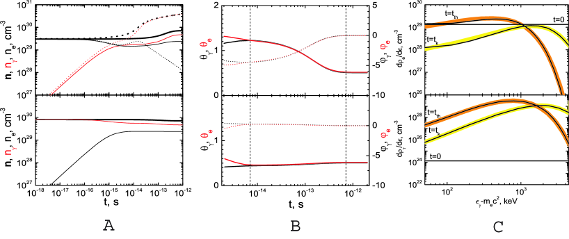
In Fig. 41, panel A concentrations of photons and pairs as well as their sum for both initial conditions are shown. After calculations begin, concentrations and energy density of photons (pairs) increase rapidly with time, due to annihilation (creation) of pairs. Then, in the kinetic equilibrium phase, concentrations of each component stay almost constant, and the sum of concentrations of photons and pairs remains unchanged. Finally, both individual components and their sum reach stationary values. If one compares and contrasts both cases as reproduced in Fig. 41 A one can see that, although the initial conditions are drastically different, in both cases the same asymptotic values of the concentration are reached.
One can see in Fig. 41, panel C that the spectral density of photons and pairs can be fitted already at sec by distribution functions (657) with definite values of temperature and chemical potential , common for pairs and photons. As expected, after the distribution functions preserve their form (657) with the values of temperature and chemical potential changing in time, as shown in Fig. 41, panel B. As one can see from this figure, the chemical potential evolves with time and reaches zero at the moment sec , corresponding to the final stationary solution. Condition (673) is satisfied in kinetic equilibrium.
The necessary condition for thermal equilibrium in the pair plasma is the detailed balance between direct and inverse triple interactions. This point is usually neglected in the literature where there are claims that the thermal equilibrium may be established with only binary interactions [491]. In order to demonstrate it explicitly in Fig. 41, panel A the dependence of concentrations of pairs and photons when inverse triple interactions are artificially switched off is also shown. In this case (see dotted curves in the upper part of Fig. 41, panel A), after kinetic equilibrium is reached concentrations of pairs decrease monotonically with time, and thermal equilibrium is never reached.
The existence of a non-null chemical potential for photons indicates the departure of the distribution function from the one corresponding to thermal equilibrium. Negative (positive) value of the chemical potential generates an increase (decrease) of the number of particles in order to approach the one corresponding to the thermal equilibrium state. Then, since the total number of particles increases (decreases), the energy is shared between more (less) particles and the temperature decreases (increases). Clearly, as thermal equilibrium is approached, the chemical potential of photons is zero.
In this example with the energy density the thermal equilibrium is reached at sec with the final temperature MeV. For a larger energy density the duration of the kinetic equilibrium phase, as well as of the thermalization timescale, is smaller. Recall, that in entire temperature range the plasma is nondegenerate.
The results, obtained for the case of an uniform plasma, can only be adopted for a description of a physical system with dimensions cm.
The assumption of the constancy of the energy density is only valid if the dynamical timescale of the plasma is much larger than the above timescale which is indeed true in all the cases of astrophysical interest.
Since thermal equilibrium is obtained already on the timescale sec, and such a state is independent of the initial distribution functions for electrons, positrons and photons, the sufficient condition to obtain an isothermal distribution on a causally disconnected spatial scale cm is the request of constancy of the energy density on such a scale as well as, of course, the invariance of the physical laws.
To summarize, the evolution of an initially nonequilibrium optically thick electron–positron-photon plasma is considered up to reaching thermal equilibrium. Starting from arbitrary initial conditions kinetic equilibrium is obtained from first principles, directly solving the relativistic Boltzmann equations with collisional integrals computed from QED matrix elements. The essential role of direct and inverse triple interactions in reaching thermal equilibrium is demonstrated. These results can be applied in the theories of the early Universe and of astrophysical sources, where thermal equilibrium is postulated at the very early stages. These results can in principle be tested in laboratory experiments in the generation of electron–positron pairs.
10 Concluding remarks
We have reviewed three fundamental quantum processes which have highlighted some of the greatest effort in theoretical and experimental physics in last seventy years. They all deal with creation and annihilation of electron–positron pairs. We have followed the original path starting from the classical works of Dirac, on the process , and the inverse process, , considered by Breit–Wheeler. We have then reviewed the pair creation in a critical electric field and the Sauter-Heisenberg-Euler-Schwinger description of this process both in Quantum Mechanics and Quantum Electro-Dynamics. We have also taken this occasion to reconstruct the exciting conceptual developments, initiated by the Sauter work, enlarged by the Born-Infeld nonlinear electrodynamical approach, finally leading to the Euler and Euler-Heisenberg results. We were guided in this reconstruction by the memories of many discussions of one of us (RR) with Werner Heisenberg. We have then reviewed the latest theoretical developments deriving the general formula for pair production rate in electric fields varying in space and in time, compared with one in a constant electric field approximation originally studied by Schwinger within QED. We also reviewed recent studies of pair production rates in selected electric fields varying both in space and in time, obtained in the literature using instanton and JWKB methods. Special attention has been given to review the pair production rate in electric fields alternating periodically in time, early derived by Brezin, Itzykson and Popov, and the nonlinear Compton effect in the processes of electrons and photons colliding with laser beams, studied by Nikishov and Narozhny. These theoretical results play an essential role in Laboratory experiments to observe the pair production phenomenon using laser technologies.
We then reviewed the different level of verification of these three processes in experiments carried all over the world. We stressed the success of experimental verification of the Dirac process, by far one of the most prolific and best tested process in the field of physics. We also recalled the study of the hadronic branch in addition to the pure electrodynamical branch originally studied by Dirac, made possible by the introduction of storage rings technology. We then turned to the very exciting current situation which sees possibly the Breit–Wheeler formula reaching its first experimental verification. This result is made possible thanks to the current great developments of laser physics. We reviewed as well the somewhat traumatic situation in the last forty years of the heavy-ion collisions in Darmstadt and Brookhaven, yet unsuccessfully attempting to observe the creation of electron–positron pairs. We also reviewed how this vast experimental program was rooted in the theoretical ideas of Zeldovich, Popov, Greiner and their schools.
We have also recalled the novelty in the field of relativistic astrophysics where we are daily observing the phenomenon of Gamma Ray Bursts [477, 516, 517, 404, 518]. These bursts of photons occur in energy range keV to MeV, last about one second and come from astrophysical sources located at a cosmological distance [394, 519, 520, 521, 522]. The energy released is up to ergs, equivalent to all the energy emitted by all the stars of all the galaxies of the entire visible Universe during that second. It is generally agreed that the energetics of these GRB sources is dominated by a dense plasma of electrons, positrons and photons created during the process of gravitational collapse leading to a Black Hole, see e.g. [68, 399, 400, 398] and references therein. The Sauter-Heisenberg-Euler-Schwinger vacuum polarization process, we have considered in the first part of the report, is a classic theoretical model to study the creation of an electron–positron optically thick plasma. Similarly the Breit–Wheeler and the Dirac processes we have discussed, are essential in describing the further evolution of such an optically thick electron–positron plasma. The GRBs present an unique opportunity to test new unexplored regime of ultrahigh energy physics with Lorentz factor and relativistic field theories in the strongest general relativistic domain.
The aim in this report, in addition to describe the above mentioned three basic quantum processes, has been to identify and review three basic relativistic regimes dealing with an optically thin and optically thick electron–positron plasma.
The first topic contains the basic results of the physics of black holes, of their energetics and of the associated process of vacuum polarization. We reviewed the procedures to generalize in a Kerr–Newman geometry the QED treatment of Schwinger and the creation of enormous number of electron–positron pairs in such a process.
The second topic is the back reaction of a newly created electron–positron plasma on an overcritical electric field. Again we reviewed the Breit–Wheeler and Dirac processes applied in the wider context of the Vlasov–Boltzmann–Maxwell equations. To discuss the back reaction of electron–positron pair on external electric fields, we reviewed semi-classical and kinetic theories describing the plasma oscillations using respectively the Dirac-Maxwell equations and the Boltzmann–Vlasov equations. We also reviewed the discussions of plasma oscillations damping due to quantum decoherence and collisions, described by respectively the quantum Boltzmann–Vlasov equation and Boltzmann–Vlasov equation with particle collisions terms. We particularly addressed the study of the influence of the collision processes on the plasma oscillations in supercritical electric field . After Compton times, the oscillating electric field is damped to its critical value with a large number of photons created. An equipartition of number and energy between electron–positron pairs and photons is reached. For the plasma oscillation with undercritical electric field , we recalled that electron–positron pairs, created by the vacuum polarization process, move as charged particles in external electric field reaching a maximum Lorentz factor at finite length of oscillations, instead of arbitrary large Lorentz factors, as traditionally assumed. Finally we point out some recent results which differentiate the case from the one with respect to the creation of the rest mass of the pair versus its kinetic energy. For the vacuum polarization process transforms the electromagnetic energy of the field mainly in the rest mass of pairs, with moderate contribution to their kinetic energy. Such phenomena, certainly fundamental on astrophysical scales, may become soon directly testable in the verification of the Breit–Wheeler process tested in laser experiments in the laboratory.
As the third topic we have reviewed the recent progress in the understanding of thermalization process of an optically thick electron–positron-photon plasma. Numerical integration of relativistic Boltzmann equation with collisional integrals for binary and triple interactions is used to follow the time evolution of such a plasma, in the range of energies per particle between 0.1 and 10 MeV, starting from arbitrary nonequilibrium configuration. It is recalled that there exist two types of equilibria in such a plasma: kinetic equilibrium, when all particles are at the same temperature, but have different nonzero chemical potential of photons, and thermal equilibrium, when chemical potentials vanish. The crucial role of direct and inverse binary and triple interactions in reaching thermal equilibrium is emphasized.
In a forthcoming report we will address how the above mentioned three relativistic processes can be applied to a variety of astrophysical systems including neutron stars formation and gravitational collapse, supernovae explosions and GRBs.
This report is dedicated to the progress of theoretical physics in extreme regimes of relativistic field theories which are on the verge of finding their experimental and observational verification in physics and astrophysics. It is then possible from our review and the many references we have given to gain a basic understanding of this new field of research. The three topics which we have reviewed are closely linked to the three quantum processes currently being tested in precision measurement in the laboratories. The experiments in the laboratories and the astrophysical observations cover complementary aspects which may facilitate a deeper and wider understanding of the nuclear and laser physics processes, of heavy-ion collisions as well as neutron stars formation and gravitational collapse, supernovae and GRBs phenomena. We shall return on such an astrophysical and observational topics in a dedicated forthcoming report.
* * *
We are witnessing in these times some enormous experimental and observational successes which are going to be the natural ground to test some of the theoretical works which we have reviewed in this report. Among the many experimental progresses being done in particle accelerators worldwide we like to give special mention to two outstanding experimental facilities which are expected to give results in the forthcoming years. We refer here to the National Ignition Facility at the Lawrence Livermore National Laboratory to be soon becoming operational, see e.g. [523] as well as the corresponding facility in France, the Mega Joule project [524].
In astrophysics these results will be tested in galactic and extragalactic black holes observed in binary X-ray sources, active galactic nuclei, microquasars and in the process of gravitational collapse to a neutron star and also of two neutron stars to a black hole in GRBs. The progress there is equally remarkable. In the last few days after the completion of this report thanks to the tremendous progress in observational technology for the first time a massive hypergiant star has been identified as the progenitor of the supernova SN 2005gl [525]. In parallel the joint success of observations of the flotilla of X-ray observatories and ground-based large telescopes [177] have allowed to identify the first object ever observed at the GRB090423 [526].
To follow the progress of this field we are planning a new report which will be directed to the astrophysical nature of the progenitors and the initial physical conditions leading to the process of the gravitational collapse. There the electrodynamical structure of neutron stars, the phenomenon of the supernova explosion as well as theories of Gamma-Ray Bursts (GRBs) will be discussed. Both in the case of neutron stars and the case of black holes there are fundamental issues still to be understood about the process of gravitational collapse especially with the electrodynamical conditions at the onset of the process. The major difficulties appear to be connected with the fact that all fundamental interactions, the gravitational, the electromagnetic, the strong, the weak interactions appear to participate in essential way to this process which appear to be therefore one of the most interesting fundamental process of theoretical physics. Current progress is presented in the following works [527, 528, 529, 530, 531, 532, 533, 534, 535, 536, 537, 538]. What is important to recall at this stage is only that both the supernovae and GRBs processes are among the most energetic and transient phenomena ever observed in the Universe: a supernova can reach energy of ergs (hypernovae) on a time scale of a few months and GRBs can have emission of up to ergs [539] in a time scale as short as of a few seconds. The central role in their description of neutron stars, for supernova as well as of black holes and the electron–positron plasma discussed in this report, for GRBs, are widely recognized. The reason which makes this last research so important can be seen in historical prospective: the Sun has been the arena to understand the thermonuclear evolution of stars [540], Cyg X-1 has evidenced the gravitational energy role in explaining an astrophysical system [541], the GRBs are promising to prove the existence for the first time of the “blackholic energy”. These three quantum processes described in our report reveal the basic phenomena in the process of gravitational collapse predicted by Einstein theory of General Relativity [177].
Notes added in proof
- •
-
•
Some new results were obtained for QED in quasi constant in time electric field, in particular, the distributions of particles created is discussed in [544, 545]; consistency restrictions on maximal electric field strength in QFT are discussed in [546]. One-loop energy-momentum tensor in QED is obtained in [547]. The exact rate of pair production by a smooth potential proportional to in three dimensions is obtained in [548].
-
•
A recent review on the muon anomalous magnetic moment (muon g-2), offers the possibility, by making most precise measurement of muon g-2 in low-energies, to infer virtual hadronic vacuum polarization and light-by-light scattering effects due to virtual quark-pairs production in high-energies. In recent BNL E821 experiment111111http://www.g-2.bnl.gov, the muon anomalous magnetic moment can be rather accurately measured. In the theory of Standard Model for elementary particles, the muon anomalous magnetic moment receive leptonic QED-contributions to , which has been calculated, see for a review [549], up to 5-loop contributions
While hadronic () contributions to the muon anomalous magnetic moment contain, due to the strong interaction, both perturbative and non-perturbative parts, the contribution to ,
where is given by
and is the vacuum polarization contribution,
and a cut in the energy, separating the non-perturvative part to be evaluated from data and the perturbative high energy tail to be calculated using perturvative QCD (pQCD), analogously to QED-calculations. The pQCD calculations may only be trusted above 2 GeV and away from threshold and resonances. In the report [549], authors resort to a semiphenomenological approach using dispersion relations together with the optical theorem and experimental data. The “measurements of ” get more difficult as increasing energies more and more channels open for meson-resonances. In addition, the most problematic set of hadronic corrections is that related to hadronic light-by-light scattering, which for the first time show up at order via the diagrams with insertion of a box with four photon lines. As a contribution to the anomalous magnetic moment three of four photons are virtual and to be integrated over all four-momentum space, such that a direct experimental input for the non-perturbative dressed four-photon correlator is not available. In this case one has to resort the low energy effective description of QCD like chiral perturbation theory (CHPT) extended to include vector-mesons, which is reviewed in detail [549]. Furthermore, the Electroweak corrections of weak virtual process including intermediate bosons and to are important and now almost three standard deviations, and without it the deviation between theory and experiment would be the level. The test of the weak contribution is actually one of the milestones achieved by Brookhaven experiment E821 (see the footnote above). These studies and experiments are crucial to include the contributions from all known particles and interactions such that from a possible deviation between theory and experiment we may get a hint of the yet unknown physics.
- •
-
•
We would like to point out that in our report, one-loop vacuum polarization and light-by-light scattering effects (effective Euler-Heisenberg Lagrangian), as well as their high-order corrections in low-energies are considered in Section 4.7; non-linear Compton effect is discussed in both Section 4.10 (theory) and Sections 6.2,6.3 (experiments); the Breit-Wheeler cutoff in high-energy -rays for astrophysics in Section 6.4. All these discussions are limited in the leptonic sector for low-energies. The reason of recording here these hadronic contributions in the high-energy region is motivated by our expectation that these effects will be possibly soon detected by direct measurements of gamma ray emission from high-energy astrophysical processes. We shall return on this topic in our forthcoming report already mentioned above.
Acknowledgment.
We would like to thank A.G. Aksenov, G. Altarelli, D. Arnett, A. Ashtekar, G. Barbiellini, V.A. Belinski, C.L. Bianco, D. Bini, P. Chardonnet, C. Cherubini, F. Fraschetti, R. Giacconi, W. Greiner, F. Guerra, R. Jantzen, G. ’t Hooft, I.B. Khriplovich, H. Kleinert, P. Menotti, S. Mercuri, N.B. Narozhny, A. Pelster, V.S. Popov, G. Preparata, B. Punsly, J. Rafelski, J. Reihardt, A. Ringwald, M. Rotondo, J. Rueda, M. Testa, L. Titarchuk, L. Vitagliano, J.R. Wilson for many important discussions.
References
- [1] P. A. M. Dirac, Annihilation of electrons and protons, Proceedings of the Cambridge Philosophical Society 26 (1930) 361–375.
- [2] G. Breit, J. A. Wheeler, Collision of Two Light Quanta, Physical Review 46 (1934) 1087–1091.
- [3] O. Klemperer, The annihilation radiation of the positron, Proceedings of the Cambridge Philosophical Society 30 (1934) 347–354.
- [4] M. Born, Modified Field Equations with a Finite Radius of the Electron, Nature132 (1933) 282–+.
- [5] M. Born, On the Quantum Theory of the Electromagnetic Field, Royal Society of London Proceedings Series A 143 (1934) 410–437.
- [6] M. Born, L. Infeld, Foundations of the New Field Theory, Royal Society of London Proceedings Series A 144 (1934) 425–451.
- [7] W. Heisenberg, H. Euler, Folgerungen aus der Diracschen Theorie des Positrons, Zeitschrift fur Physik 98 (1936) 714–732.
- [8] S. Tomonaga, On a Relativistically Invariant Formulation of the Quantum Theory of Wave Fields, Progress of Theoretical Physics 1 (1946) 27–42.
- [9] R. P. Feynman, Space-Time Approach to Non-Relativistic Quantum Mechanics, Reviews of Modern Physics 20 (1948) 367–387.
- [10] R. P. Feynman, The Theory of Positrons, Physical Review 76 (1949) 749–759.
- [11] R. P. Feynman, Space-Time Approach to Quantum Electrodynamics, Physical Review 76 (1949) 769–789.
- [12] J. Schwinger, Quantum Electrodynamics. I. A Covariant Formulation, Physical Review 74 (1948) 1439–1461.
- [13] J. Schwinger, Quantum Electrodynamics. II. Vacuum Polarization and Self-Energy, Physical Review 75 (1949) 651–679.
- [14] J. Schwinger, Quantum Electrodynamics. III. The Electromagnetic Properties of the Electron-Radiative Corrections to Scattering, Physical Review 76 (1949) 790–817.
- [15] F. J. Dyson, The Radiation Theories of Tomonaga, Schwinger, and Feynman, Physical Review 75 (1949) 486–502.
- [16] F. J. Dyson, The S Matrix in Quantum Electrodynamics, Physical Review 75 (1949) 1736–1755.
- [17] O. Klein, Die Reflexion von Elektronen an einem Potentialsprung nach der relativistischen Dynamik von Dirac, Zeitschrift fur Physik 53 (1929) 157–165.
- [18] F. Sauter, Zum ”Kleinschen Paradoxon”., Zeitschrift fur Physik 73 (1931) 547–+.
- [19] G. Gamow, Constitution of Atomic Nuclei And Radioactivity, Oxford University Press, 1931.
- [20] F. Sauter, Über das Verhalten eines Elektrons im homogenen elektrischen Feld nach der relativistischen Theorie Diracs, Zeitschrift fur Physik 69 (1931) 742–764.
- [21] H. Euler, Über die Streuung von Licht an Licht nach der Diracschen Theorie, Annalen der Physik 418 (1936) 398–448.
- [22] B. Hoffmann, Gravitational and Electromagnetic Mass in the Born-Infeld Electrodynamics, Physical Review 47 (1935) 877–880.
- [23] B. Hoffmann, L. Infeld, On the Choice of the Action Function in the New Field Theory, Physical Review 51 (1937) 765–773.
- [24] V. Weisskopf, Kongelige Danske Videnskabernes Selskab 14 (1936) 6.
- [25] J. Schwinger, On Gauge Invariance and Vacuum Polarization, Physical Review 82 (1951) 664–679.
- [26] J. Schwinger, The Theory of Quantized Fields. V, Physical Review 93 (1954) 615–628.
- [27] J. Schwinger, The Theory of Quantized Fields. VI, Physical Review 94 (1954) 1362–1384.
- [28] A. I. Nikishov, JETP 30 (1969) 660–+.
- [29] V. S. Vanyashin, M. V. Terent’ev, The Vacuum Polarization of a Charged Vector Field, Soviet Journal of Experimental and Theoretical Physics 21 (1965) 375–+.
- [30] V. S. Popov, Production of Pairs in an Alternating External Field, ZhETF Pis ma Redaktsiiu 13 (1971) 261–+.
- [31] V. S. Popov, Pair Production in a Variable External Field (Quasiclassical Approximation), Soviet Journal of Experimental and Theoretical Physics 34 (1972) 709–+.
- [32] V. S. Popov, Schwinger Mechanism of Electron-Positron Pair Production by the Field of Optical and X-ray Lasers in Vacuum, Soviet Journal of Experimental and Theoretical Physics Letters 74 (2001) 133–138.
- [33] N. B. Narozhnyi, A. I. Nikishov, The Simplist processes in the pair creating electric field, Yad. Fiz. 11 (1970) 1072.
- [34] I. A. Batalin, E. S. Fradkin, Quantum electrodynamics in external fields. I, Theoretical and Mathematical Physics 5 (1970) 1080–1100.
- [35] R. Ruffini, S. Xue, J. of Korean Phys. Soc. 49 (2006) 715.
- [36] E. Brezin, C. Itzykson, Pair Production in Vacuum by an Alternating Field, Phys. Rev. D2 (1970) 1191–1199.
- [37] V. S. Popov, Pair Production in a Variable and Homogeneous Electric Field as an Oscillator Problem, Soviet Journal of Experimental and Theoretical Physics 35 (1972) 659–+.
- [38] C. Bula, K. T. McDonald, E. J. Prebys, C. Bamber, S. Boege, T. Kotseroglou, A. C. Melissinos, D. D. Meyerhofer, W. Ragg, D. L. Burke, R. C. Field, G. Horton-Smith, A. C. Odian, J. E. Spencer, D. Walz, S. C. Berridge, W. M. Bugg, K. Shmakov, A. W. Weidemann, Observation of Nonlinear Effects in Compton Scattering, Physical Review Letters 76 (1996) 3116–3119.
- [39] D. L. Burke, R. C. Field, G. Horton-Smith, J. E. Spencer, D. Walz, S. C. Berridge, W. M. Bugg, K. Shmakov, A. W. Weidemann, C. Bula, K. T. McDonald, E. J. Prebys, C. Bamber, S. J. Boege, T. Koffas, T. Kotseroglou, A. C. Melissinos, D. D. Meyerhofer, D. A. Reis, W. Ragg, Positron Production in Multiphoton Light-by-Light Scattering, Physical Review Letters 79 (1997) 1626–1629.
- [40] A. I. Nikishov, V. I. Ritus, Sov. Phys. JETP 19 (1964) 529.
- [41] A. I. Nikishov, V. I. Ritus, Sov. Phys. JETP 19 (1964) 1191.
- [42] A. I. Nikishov, V. I. Ritus, Sov. Phys. JETP 20 (1965) 757.
- [43] A. I. Nikishov, V. I. Ritus, Pair Production by a Photon and Photon Emission by an Electron in the Field of an Intense Electromagnetic Wave and in a Constant Field, Soviet Journal of Experimental and Theoretical Physics 25 (1967) 1135–+.
- [44] A. I. Nikishov, V. I. Ritus, Proc. (Tr.) P. N. Lebedev Phys. Inst. Acad. Sci. USSR 111.
- [45] A. I. Nikishov, V. I. Ritus, Sov. Phys. JETP 20 (1965) 622.
- [46] I. B. Khriplovich, Charged-particle creation by charged black holes, Nuovo Cimento B Serie 115 (2000) 761–+.
- [47] C. Schubert, Perturbative quantum field theory in the string-inspired formalism, Phys. Rep.355 (2001) 73–234.
- [48] G. V. Dunne, C. Schubert, Worldline instantons and pair production in inhomogenous fields, Phys. Rev. D72 (10) (2005) 105004–+. arXiv:arXiv:hep-th/0507174.
- [49] G. V. Dunne, Q.-H. Wang, H. Gies, C. Schubert, Worldline instantons and the fluctuation prefactor, Phys. Rev. D73 (6) (2006) 065028–+. arXiv:arXiv:hep-th/0602176.
- [50] G. V. Dunne, Q.-H. Wang, Multidimensional worldline instantons, Phys. Rev. D74 (6) (2006) 065015–+. arXiv:arXiv:hep-th/0608020.
- [51] S. P. Kim, D. N. Page, Schwinger pair production via instantons in strong electric fields, Phys. Rev. D65 (10) (2002) 105002–+. arXiv:arXiv:hep-th/0005078.
- [52] S. P. Kim, D. N. Page, Schwinger pair production in electric and magnetic fields, Phys. Rev. D73 (6) (2006) 065020–+. arXiv:arXiv:hep-th/0301132.
- [53] S. P. Kim, D. N. Page, Improved approximations for fermion pair production in inhomogeneous electric fields, Phys. Rev. D75 (4) (2007) 045013–+. arXiv:arXiv:hep-th/0701047.
-
[54]
H. Kleinert, R. Ruffini, S.-S. Xue,
Electron-positron pair
production in space- or time-dependent electric fields, Physical Review D
(Particles, Fields, Gravitation, and Cosmology) 78 (2) (2008) 025011.
URL http://link.aps.org/abstract/PRD/v78/e025011 - [55] C. Bernardini, AdA:The First Electron-Positron Collider, Physics in Perspective 6 (2004) 156–183.
- [56] A. I. Nikishov, Absorption of high-energy photons in the universe, Zhurnal Eksperimental’noi i Teoreticheskoi Fiziki 41 (1961) 549–550.
- [57] D. A. G. Deacon, L. R. Elias, J. M. J. Madey, G. J. Ramian, H. A. Schwettman, T. I. Smith, First operation of a free-electron laser, Physical Review Letters 38 (1977) 892–894.
- [58] A. Tremaine, X. J. Wang, M. Babzien, I. Ben-Zvi, M. Cornacchia, H.-D. Nuhn, R. Malone, A. Murokh, C. Pellegrini, S. Reiche, J. Rosenzweig, V. Yakimenko, Experimental Characterization of Nonlinear Harmonic Radiation from a Visible Self-Amplified Spontaneous Emission Free-Electron Laser at Saturation, Physical Review Letters 88 (20) (2002) 204801–+.
-
[59]
H.-D. Nuhn, C. Pellegrini,
Proceedings of the x-ray fel theory and simulation codes workshop (2000).
URL http://www-ssrl.slac.stanford.edu/lcls/technotes/LCLS-TN-00-1.pdf - [60] A. Ringwald, Pair production from vacuum at the focus of an X-ray free electron laser, Physics Letters B 510 (2001) 107–116. arXiv:arXiv:hep-ph/0103185.
- [61] H. R. Reiss, Absorption of Light by Light, Journal of Mathematical Physics 3 (1962) 59–67.
- [62] H. R. Reiss, Production of Electron Pairs from a Zero-Mass State, Physical Review Letters 26 (1971) 1072–1075.
- [63] T. Kotseroglou, C. Bamber, S. Boege, A. C. Melissinos, D. D. Meyerhofer, W. Ragg, C. Bula, K. T. McDonald, E. J. Prebys, D. Bernstein, D. Burke, E. Cisneros, R. C. Field, G. Horton-Smith, K. Jobe, J. Judkins, A. C. Odian, M. Ross, D. Waltz, S. C. Berridge, W. M. Bugg, K. Shmakov, A. W. Weidemann, Picosecond timing of terawatt laser pulses with the SLAC 46 GeV electron beam, Nuclear Instruments and Methods in Physics Research A 383 (1996) 309–317.
- [64] I. Y. Pomeranchuk, Y. Smorodinskii, Energy levels of systems with z greater than 137, Journal of Physics (USSR) 9 (1945) 97–100.
- [65] Y. B. Zeldovich, V. S. Popov, Electronic Structure of Superheavy Atoms, Soviet Physics Uspekhi 14 (1971) 673–+.
- [66] W. Greiner, J. Reinhardt, Supercritical fields in heavy ion physics - a status report, in: P. Chen (Ed.), Quantum Aspects of Beam Physics, World Scientific, 1999, pp. 438–463, proceedings of the 15th Advanced ICFA Beam Dynamics Workshop on Quantum Aspects of Beam Physics, Monterey, California, 4-9 Jan 1998.
- [67] B. Carter, Hamilton-jacobi and schrodinger separable solutions of einstein’s equations, Communications in Mathematical Physics 10 (1968) 280–310.
- [68] T. Damour, R. Ruffini, Quantum electrodynamical effects in Kerr-Newman geometries., Physical Review Letters 35 (1975) 463–466.
- [69] J. R. Oppenheimer, H. Snyder, On Continued Gravitational Contraction, Physical Review 56 (1939) 455–459.
- [70] W. Israel, Singular hypersurfaces and thin shells in general relativity, Nuovo Cimento B Serie 44 (1966) 1–14.
- [71] V. De la Cruz, W. Israel, Gravitational bounce, Nuovo Cimento A Serie 51 (1967) 744–760.
- [72] R. Ruffini, L. Vitagliano, S.-S. Xue, On plasma oscillations in strong electric fields, Phys. Lett. B 559 (2003) 12–19. arXiv:arXiv:astro-ph/0302549.
- [73] R. Ruffini, G. V. Vereshchagin, S.-S. Xue, Vacuum polarization and plasma oscillations, Phys. Lett. A 371 (2007) 399–405. arXiv:arXiv:0706.4363.
- [74] A. G. Aksenov, R. Ruffini, G. V. Vereshchagin, Thermalization of Nonequilibrium Electron-Positron-Photon Plasmas, Phys. Rev. Lett.99 (12) (2007) 125003–+. arXiv:arXiv:0707.3250.
- [75] A. G. Aksenov, R. Ruffini, G. V. Vereshchagin, Thermalization of Electron-Positron-Photon Plasmas with an application to GRB, in: American Institute of Physics Conference Series, Vol. 966 of American Institute of Physics Conference Series, 2008, pp. 191–196.
- [76] J. Ehlers, Survey of general relativity theory, in: Relativity, Astrophysics and Cosmology, 1973, pp. 1–125.
- [77] G. Cavallo, M. J. Rees, A qualitative study of cosmic fireballs and gamma-ray bursts, MNRAS183 (1978) 359–365.
-
[78]
B. V. Medvedev, D. V. Shirkov,
P. a. m. dirac and the
formation of the basic ideas of quantum field theory, Soviet Physics Uspekhi
30 (9) (1987) 791–815.
URL http://stacks.iop.org/0038-5670/30/791 - [79] A. I. Miller, Early Quantum Electrodynamics, Early Quantum Electrodynamics, Edited by Arthur I. Miller, pp. 285. ISBN 0521568919. Cambridge, UK: Cambridge University Press, October 1995., 1995.
- [80] P. A. M. Dirac, The Quantum Theory of the Electron, Royal Society of London Proceedings Series A 117 (1928) 610–624.
- [81] P. A. M. Dirac, A Theory of Electrons and Protons, Royal Society of London Proceedings Series A 126 (1930) 360–365.
- [82] P. A. M. Dirac, Quantised Singularities in the Electromagnetic Field, Royal Society of London Proceedings Series A 133 (1931) 60–72.
- [83] C. D. Anderson, Energies of Cosmic-Ray Particles, Physical Review 41 (1932) 405–421.
- [84] C. D. Anderson, The Positive Electron, Physical Review 43 (1933) 491–494.
- [85] J. Mehra, H. Rechenberg, The historical development of quantum theory, 1982.
- [86] P. A. M. Dirac, On the Theory of Quantum Mechanics, Royal Society of London Proceedings Series A 112 (1926) 661–677.
- [87] W. Heitler, Quantum theory of radiation, International Series of Monographs on Physics, Oxford: Clarendon, 1954, 3rd ed., 1954.
- [88] L. D. Landau, E. M. Lifshitz, Non-Relativistic Quantum Mechanics, Elsevier, 1981.
- [89] C. Itzykson, J.-B. Zuber, Quantum Field Theory, Dover Publications, 2006.
- [90] V. B. Berestetskii, E. M. Lifshitz, V. B. Pitaevskii, Quantum Electrodynamics, Elsevier, 1982.
- [91] P. M. S. Blackett, G. P. S. Occhialini, Some Photographs of the Tracks of Penetrating Radiation, Royal Society of London Proceedings Series A 139 (1933) 699–720.
-
[92]
[link].
URL http://www.time.com/time/magazine/article/0,9171,753401,00.html - [93] I. Curie, F. Joliot, Emission de protons de grande vitesse par les substances hydrogenees sous l influence des rayons gamma tres penetrants, C.R. Acad. Sci. 194 (1932) 708–711.
- [94] J. R. Oppenheimer, M. S. Plesset, On the Production of the Positive Electron, Physical Review 44 (1933) 53–55.
- [95] W. Heitler, Über die bei sehr schnellen Stößen emittierte Strahlung, Zeitschrift fur Physik 84 (1933) 145–167.
- [96] H. Bethe, W. Heitler, On the Stopping of Fast Particles and on the Creation of Positive Electrons, Royal Society of London Proceedings Series A 146 (1934) 83–112.
- [97] F. Sauter, Über die Bremsstrahlung schneller Elektronen, Annalen der Physik 412 (1934) 404–412.
- [98] G. Racah, Sulla nascita degli elettroni positivi, Il Nuovo Cimento 11 (1934) 477–481.
- [99] L. D. Landau, E. M. Lifshitz, On creation of electrons and positrons in collision of two particles, Physikalische Zeitschrift der Sowjetunion 6 (1934) 244–236.
- [100] G. Racah, Sulla nascita di coppie per urti di particelle elettrizzate, Il Nuovo Cimento 14 (1937) 93–113.
- [101] V. M. Budnev, I. F. Ginzburg, G. V. Meledin, V. G. Serbo, The two-photon particle production mechanism. Physical problems. Applications. Equivalent photon approximation, Phys. Rep.15 (1975) 181–282.
- [102] H. J. Bhabha, The Creation of Electron Pairs by Fast Charged Particles, Royal Society of London Proceedings Series A 152 (1935) 559–586.
- [103] A. Sommerfeld, Über die Beugung und Bremsung der Elektronen, Annalen der Physik 403 (1931) 257–330.
- [104] C. A. Bertulani, S. R. Klein, J. Nystrand, Physics of Ultra-Peripheral Nuclear Collisions, Annual Review of Nuclear and Particle Science 55 (2005) 271–310. arXiv:arXiv:nucl-ex/0502005.
- [105] E. Fermi, On the theory of collisions between atoms and elastically charged particles, Zeitschrift fur Physik 29 (1924) 315.
- [106] C. F. V. Weizsäcker, Ausstrahlung bei Stößen sehr schneller Elektronen, Zeitschrift fur Physik 88 (1934) 612–625.
- [107] E. J. Williams, Nature of the High Energy Particles of Penetrating Radiation and Status of Ionization and Radiation Formulae, Physical Review 45 (1934) 729–730.
- [108] H. A. Olsen, Improved Weizsäcker-Williams method, Phys. Rev. D19 (1979) 100–103.
- [109] E. Schrödinger, Quantisierung als Eigenwertproblem, Annalen der Physik 386 (1926) 109–139.
- [110] V. Fock, Über die invariante Form der Wellen- und der Bewegungsgleichungen für einen geladenen Massenpunkt, Zeitschrift fur Physik 39 (1926) 226–232.
- [111] O. Klein, Quantentheorie und fünfdimensionale Relativitätstheorie, Zeitschrift fur Physik 37 (1926) 895–906.
- [112] W. Gordon, Der Comptoneffekt nach der Schrödingerschen Theorie, Zeitschrift fur Physik 40 (1926) 117–133.
- [113] T. Damour, , in: Marcel Grossmann Meeting: General Relativity, 1975, pp. 459–+.
- [114] L. D. Landau, E. M. Lifshitz, The classical theory of fields, Course of theoretical physics - Pergamon International Library of Science, Technology, Engineering and Social Studies, Oxford: Pergamon Press, 1975, 4th rev.engl.ed., 1975.
- [115] J. Schwinger, On Quantum-Electrodynamics and the Magnetic Moment of the Electron, Physical Review 73 (1948) 416–417.
- [116] B. E. Lautrup, A. Peterman, E. de Rafael, Recent developments in the comparison between theory and experiments in quantum electrodynamics, Phys. Rep.3 (1972) 193–259.
- [117] P. Cvitanović, T. Kinoshita, Sixth-order magnetic moment of the electron, Phys. Rev. D10 (1974) 4007–4031.
- [118] J. Bailey, K. Borer, F. Combley, H. Drumm, F. J. M. Farley, J. H. Field, W. Flegel, P. M. Hattersley, F. Krienen, F. Lange, E. Picasso, W. Von Rüden, The anomalous magnetic moment of positive and negative muons, Physics Letters B 68 (1977) 191–196.
- [119] O. Halpern, Scattering Processes Produced by Electrons in Negative Energy States, Physical Review 44 (1933) 855–856.
- [120] P. Debye, in discussion with Heisenberg (1934).
- [121] W. Pauli, Theory of Relativity, Dover Publications, 1981.
- [122] G. Mie, Grundlagen einer Theorie der Materie, Annalen der Physik 344 (1912) 1–40.
- [123] G. Mie, Grundlagen einer Theorie der Materie, Annalen der Physik 342 (1912) 511–534.
- [124] G. Mie, Grundlagen einer Theorie der Materie, Annalen der Physik 345 (1913) 1–66.
- [125] M. Born, Der Impuls-Energie-Satz in der Elektrodynamik von Gustav Mie, Nachrichten der Akademie der Wissenschaften in Göttingen. Mathematisch-Physikalische Klasse (1914) 23.
- [126] A. Einstein, L. Infeld, Evolution of Physics, Touchstone, 1967.
-
[127]
A. Einstein, L. Infeld, B. Hoffmann,
The gravitational equations and
the problem of motion, The Annals of Mathematics 39 (1) (1938) 65–100.
URL http://www.jstor.org/stable/1968714 - [128] H. Euler, B. Kockel, Über die Streuung von Licht an Licht nach der Diracschen Theorie, Naturwissenschaften 23 (1935) 246–247.
- [129] L. D. Landau, E. M. Lifshitz, Electrodynamics of continuous media, Energy Conversion Management, 1960.
- [130] P. A. M. Dirac, Infinite distribution of electrons in the theory of the positron, Proceedings of the Cambridge Philosophical Society 30 (1934) 150–163.
- [131] W. Heisenberg, Bemerkungen zur Diracschen Theorie des Positrons, Zeitschrift fur Physik 90 (1934) 209–231.
- [132] V. Weisskopf, Über die Selbstenergie des Elektrons, Zeitschrift fur Physik 89 (1934) 27–39.
- [133] J. Schwinger, Selected Papers on Quantum Electrodynamics, Dover Publications, 1958.
- [134] N. N. Bogoliubov, D. V. Shirkov, Introduction to the theory of quantized fields, Introduction to the theory of quantized fields, by Bogoli’ubov, N. N.; Shirkov, D. V. New York, Interscience Publishers, 1959. Interscience monographs in physics and astronomy ; v. 3, 1959.
- [135] J. Bjorken, S. Drell, Relativistic Quantum Mechanics, McGraw-Hill Science, 1998.
- [136] J. Bjorken, S. Drell, Relativistic Quantum Fields, Mcgraw-Hill College, 1965.
- [137] R. Feynman, Quantum Electrodynamics, Westview Press, 1998.
- [138] R. Feynman, A. Hibbs, Quantum Mechanics and Path Integrals, McGraw-Hill Companies, 1965.
- [139] T. D. Lee, Particle Physics and Introduction to Field Theory, Harwood Academic Publishers, 1990.
- [140] J. Schwinger, Particles Sources and Fields, ADDISON WESLEY, 1970.
- [141] J. Schwinger, Particles, Sources, and Fields: Vol. 2, Westview Press, 1998.
- [142] S. Weinberg, The quantum theory of fields. Vol.1: Foundations, Cambridge, New York: Cambridge University Press, —c1995, 1995.
- [143] H. Kleinert, Gauge Fields in Condensed Matter, World Scientific, 1990.
- [144] R. Streater, A. Wightman, PCT, Spin and Statistics, and All That, Princeton University Press, 2000.
-
[145]
H. Kleinert,
Particles and
quantum fields (2008).
URL http://users.physik.fu-berlin.de/ kleinert/b6/psfiles/ - [146] W. E. Lamb, R. C. Retherford, Fine Structure of the Hydrogen Atom by a Microwave Method, Physical Review 72 (1947) 241–243.
- [147] S. Triebwasser, E. S. Dayhoff, W. E. Lamb, Fine Structure of the Hydrogen Atom. V, Physical Review 89 (1953) 98–106.
-
[148]
The l3 experiment at cern.
URL http://l3.web.cern.ch/l3/ - [149] H. B. G. Casimir, Proc. Koninkl. Ned. Akad. Wetenschap. 51 (1948) 793.
- [150] M. Fierz, Zur anziehung leitender ebenen im vakuum, Helvetica Physica Acta 33 (1960) 855–858.
- [151] M. J. Sparnaay, Measurements of attractive forces between flat plates, Physica 24 (1958) 751–764.
- [152] S. K. Lamoreaux, Demonstration of the Casimir Force in the 0.6 to 6 m Range, Physical Review Letters 78 (1997) 5–8.
- [153] U. Mohideen, A. Roy, Precision Measurement of the Casimir Force from 0.1 to 0.9 m, Physical Review Letters 81 (1998) 4549–4552. arXiv:arXiv:physics/9805038.
- [154] J. S. Høye, I. Brevik, J. B. Aarseth, Casimir problem of spherical dielectrics: Quantum statistical and field theoretical approaches, Phys. Rev. E63 (5) (2001) 051101–+. arXiv:arXiv:quant-ph/0008088.
- [155] B. W. Harris, F. Chen, U. Mohideen, Precision measurement of the Casimir force using gold surfaces, Phys. Rev. A62 (5) (2000) 052109–+. arXiv:arXiv:quant-ph/0005088.
- [156] F. Chen, G. L. Klimchitskaya, U. Mohideen, V. M. Mostepanenko, Theory confronts experiment in the Casimir force measurements: Quantification of errors and precision, Phys. Rev. A69 (2) (2004) 022117–+. arXiv:arXiv:quant-ph/0401153.
- [157] S.-S. Xue, RADIATIVE CORRECTION TO CASIMIR EFFECT, Commun. Theor. Phys. 11 (1989) 243–248.
- [158] S.-S. Xue, CASIMIR EFFECT OF SCALAR FIELD ON S(n-1) MANIFOLD, Commun. Theor. Phys. 12 (1989) 209–218.
- [159] S.-S. Xue, D.-C. Xian, The Casimir effect in a gauge covariant field theory, Acta Physica Sinica 34 (1986) 1084–1087.
- [160] T. Zheng, S.-S. Xue, The casimir effect in perfectly conducting rectangular cavity, Chinese Science Bulletin 38 (1993) 631–635.
- [161] J. Schwinger, Casimir Energy for Dielectrics, Proceedings of the National Academy of Science 89 (1992) 4091–4093.
- [162] J. Schwinger, Casimir Energy for Dielectrics: Spherical Geometry, Proceedings of the National Academy of Science 89 (1992) 11118–11120.
- [163] J. Schwinger, Casimir Light: A Glimpse, Proceedings of the National Academy of Science 90 (1993) 958–959.
- [164] J. Schwinger, Casimir Light: The Source, Proceedings of the National Academy of Science 90 (1993) 2105–2106.
- [165] J. Schwinger, Casimir Light: Photon Pairs, Proceedings of the National Academy of Science 90 (1993) 4505–4507.
- [166] J. Schwinger, Casimir Light: Pieces of the Action, Proceedings of the National Academy of Science 90 (1993) 7285–7287.
- [167] J. Schwinger, Casimir Light: Field Pressure, Proceedings of the National Academy of Science 91 (1994) 6473–6475.
- [168] M. Bordag, Casimir Effect 50 Years Later, World Scientific Publishing Company, 1999.
- [169] M. Bordag, Quantum Field Theory Under the Influence of External Conditions, B.G.Teubner GmbH, 1996.
- [170] K. A. Milton, TOPICAL REVIEW: The Casimir effect: recent controversies and progress, Journal of Physics A Mathematical General 37 (2004) 209–+. arXiv:arXiv:hep-th/0406024.
- [171] K. Milton, The Casimir Effect, World Scientific Publishing Company, 2001.
- [172] S.-S. Xue, Possible vacuum-energy releasing, Physics Letters B 508 (2001) 211–215. arXiv:arXiv:hep-ph/0011327.
- [173] S.-S. Xue, Magnetically induced vacuum decay, Phys. Rev. D68 (1) (2003) 013004–+. arXiv:arXiv:quant-ph/0106076.
- [174] S.-S. Xue, The Dynamical Casimir Effect and Energetic Sources for Gamma Ray Bursts, Modern Physics Letters A 18 (2003) 1325–1330. arXiv:arXiv:astro-ph/0210069.
- [175] S.-S. Xue, On quantum radiation in curved spacetime, General Relativity and Gravitation 37 (2005) 857–872. arXiv:arXiv:hep-th/0204060.
- [176] O. Klein, T. Nishina, Über die Streuung von Strahlung durch freie Elektronen nach der neuen relativistischen Quantendynamik von Dirac, Zeitschrift fur Physik 52 (1929) 853–868.
- [177] R. Ruffini, The Kerr Spacetime: Rotating Black Holes in General Relativity, Cambridge Univ. Press, Cambridge, 2009, Ch. The ergosphere and dyadosphere of the Kerr black hole, p. 161.
- [178] H. Cheng, T. T. Wu, High-Energy Elastic Scattering in Quantum Electrodynamics, Physical Review Letters 22 (1969) 666–669.
- [179] H. Cheng, T. T. Wu, Longitudinal Momentum Distribution of Pionization Products, Physical Review Letters 23 (1969) 1311–1313.
- [180] H. Cheng, T. T. Wu, High-Energy Collision Processes in Quantum Electrodynamics. I, Physical Review 182 (1969) 1852–1867.
- [181] H. Cheng, T. T. Wu, High-Energy Collision Processes in Quantum Electrodynamics. II, Physical Review 182 (1969) 1868–1872.
- [182] H. Cheng, T. T. Wu, High-Energy Collision Processes in Quantum Electrodynamics. III, Physical Review 182 (1969) 1873–1898.
- [183] H. Cheng, T. T. Wu, High-Energy Collision Processes in Quantum Electrodynamics. IV, Physical Review 182 (1969) 1899–1906.
- [184] H. Cheng, T. T. Wu, Photon-Photon Scattering close to the Forward Direction, Phys. Rev. D1 (1970) 3414–3415.
- [185] H. Cheng, T. T. Wu, Elastic Scattering Processes in Scalar Electrodynamics at High Energies. I, Phys. Rev. D1 (1970) 467–473.
- [186] H. Cheng, T. T. Wu, Cross Sections for Two-Pair Production at Infinite Energy, Phys. Rev. D2 (1970) 2103–2104.
- [187] H. A. Bethe, L. C. Maximon, Theory of Bremsstrahlung and Pair Production. I. Differential Cross Section, Physical Review 93 (1954) 768–784.
- [188] H. Davies, H. A. Bethe, L. C. Maximon, Theory of Bremsstrahlung and Pair Production. II. Integral Cross Section for Pair Production, Physical Review 93 (1954) 788–795.
- [189] G. Baur, K. Hencken, D. Trautmann, Electron positron pair production in ultrarelativistic heavy ion collisions, Phys. Rep.453 (2007) 1–27. arXiv:0706.0654.
- [190] E. Bartos, S. R. Gevorkyan, E. A. Kuraev, N. N. Nikolaev, Multiple lepton pair production in relativistic ion collisions, Physics Letters B 538 (2002) 45–51. arXiv:arXiv:hep-ph/0204327.
- [191] E. Bartos, S. R. Gevorkyan, E. A. Kuraev, N. N. Nikolaev, Lepton pair production in heavy-ion collisions in perturbation theory, Phys. Rev. A66 (4) (2002) 042720–+. arXiv:arXiv:hep-ph/0109281.
- [192] O. O. Voskresenskaya, A. N. Sissakian, A. V. Tarasov, G. T. Torosyan, Watson representation for the amplitude of lepton-pair production in nucleus-nucleus collisions, Physics of Particles and Nuclei Letters 3 (2006) 246–248.
- [193] O. O. Voskresenskaya, A. N. Sissakian, A. V. Tarasov, G. T. Torosyan, The structure of the amplitude process outside the born approximation framework, Physics of Particles and Nuclei Letters 4 (2007) 18–21.
- [194] S. R. Gevorkyan, E. A. Kuraev, Lepton pair production in relativistic ion collisions to all orders in Z with logarithmic accuracy, Journal of Physics G Nuclear Physics 29 (2003) 1227–1235. arXiv:arXiv:hep-ph/0302238.
- [195] D. Ivanov, K. Melnikov, Lepton pair production by a high energy photon in a strong electromagnetic field, Phys. Rev. D57 (1998) 4025–4034. arXiv:arXiv:hep-ph/9709352.
- [196] V. G. Gorshkov, REVIEWS OF TOPICAL PROBLEMS: Electrodynamic processes in colliding beams of high-energy particles, Soviet Physics Uspekhi 16 (1973) 322–338.
- [197] V. E. Balakin, A. D. Bukin, E. V. Pakhtusova, V. A. Sidorov, A. G. Khabakhpashev, Evidence for electron-positron pair electroproduction, Physics Letters B 34 (1971) 663–664.
- [198] C. e. a. Bacci, Lett. Nuovo Cimento 3 (1972) 709.
- [199] G. Barbiellini, S. Orito, T. Tsuru, R. Visentin, F. Ceradini, M. Conversi, S. D’Angelo, M. L. Ferrer, L. Paoluzi, R. Santonico, Muon Pair Production by Photon-Photon Interactions in Storage Rings, Physical Review Letters 32 (1974) 385–388.
- [200] S. Orito, M. L. Ferrer, L. Paoluzi, R. Santonico, Two-photon annihilation into pion pair, Physics Letters B 48 (1974) 380–384.
- [201] G. Barbiellini, The early experiments on photon-photon collisions, in: G. Cochard, P. Kessler (Eds.), Photon-Photon Collisions, Vol. 134 of Lecture Notes in Physics, Berlin Springer Verlag, 1980, pp. 9–18.
- [202] H. Kleinert, Path integrals in quantum mechanics, statistics polymer physics, and financial markets, World Scientific, 2004.
- [203] W. Greiner, B. Muller, J. Rafelski, Quantum Electrodynamics of Strong Fields, Berlin, Springer, 1985.
- [204] A. Grib, S. Mamaev, V. Mostepanenko, Vacuum Quantum Effects in Strong External Fields, Moscow, Atomizdat, 1980.
- [205] E. Fradkin, D. Gitman, S. S. M., Quantum Electrodynamics: With Unstable Vacuum, Springer, 1991.
- [206] I. S. Gradshteyn, I. M. Ryzhik, Table of integrals, series and products, New York: Academic Press, —c1994, 5th ed. completely reset, edited by Jeffrey, Alan, 1994.
- [207] G. V. Dunne, Heisenberg-Euler effective Lagrangians: Basics and extensionsarXiv:hep-th/0406216.
- [208] G. V. Dunne, C. Schubert, Two-loop Euler-Heisenberg QED pair-production rate, Nuclear Physics B 564 (2000) 591–604. arXiv:arXiv:hep-th/9907190.
- [209] M. S. Marinov, V. S. Popov, Effect of Screening on the Critical Charge of a Nucleus, Soviet Journal of Experimental and Theoretical Physics Letters 17 (1973) 368–+.
- [210] M. S. Marinov, V. S. Popov, Electron-positron pair creation from vacuum induced by variable electric field, Fortschritte der Physik 25 (1977) 373–400.
- [211] C. Bamber, S. J. Boege, T. Koffas, T. Kotseroglou, A. C. Melissinos, D. D. Meyerhofer, D. A. Reis, W. Ragg, C. Bula, K. T. McDonald, E. J. Prebys, D. L. Burke, R. C. Field, G. Horton-Smith, J. E. Spencer, D. Walz, S. C. Berridge, W. M. Bugg, K. Shmakov, A. W. Weidemann, Studies of nonlinear QED in collisions of 46.6 GeV electrons with intense laser pulses, Phys. Rev. D60 (9) (1999) 092004–+.
- [212] N. Sengupta, Bull. Calcutta Math. Soc. 44.
- [213] L. S. Brown, T. W. Kibble, Interaction of Intense Laser Beams with Electrons, Physical Review 133 (1964) 705–719.
- [214] I. Goldman, Sov. Phys. JETP 19 (1964) 954.
- [215] I. Goldman, Intensity effects in compton scattering, Physics Letters 8 (1964) 103–106.
- [216] J. H. Eberly, Progress in Optics, Vol. 7, North-Holland, Amsterdam, 1969, p. 360.
- [217] D. Wolkow, ber eine klasse von l sungen der diracschen gleichung, Zeitschrift f r Physik 94 (1935) 250–260.
- [218] C. Martin, D. Vautherin, Finite-size effects in pair production by an external field, Phys. Rev. D38 (1988) 3593–3595.
- [219] C. Martin, D. Vautherin, Finite-size and dynamical effects in pair production by an external field, Phys. Rev. D40 (1989) 1667–1673.
- [220] T. N. Tomaras, N. C. Tsamis, R. P. Woodard, Back reaction in light cone QED, Phys. Rev. D62 (12) (2000) 125005–+. arXiv:arXiv:hep-ph/0007166.
- [221] J. Avan, H. M. Fried, Y. Gabellini, Nontrivial generalizations of the Schwinger pair production result, Phys. Rev. D67 (1) (2003) 016003–+. arXiv:arXiv:hep-th/0208053.
- [222] J. Rafelski, L. P. Fulcher, A. Klein, Fermions and bosons interacting with arbitrarily strong external fields, Phys. Rep.38 (1978) 227–361.
- [223] G. Soff, B. Müller, J. Rafelski, Precise Values for Critical fields in Quantum Electrodynamics, Zeitschrift Naturforschung Teil A 29 (1974) 1267–+.
- [224] R.-C. Wang, C.-Y. Wong, Finite-size effect in the Schwinger particle-production mechanism, Phys. Rev. D38 (1988) 348–359.
- [225] H. Gies, K. Langfeld, Quantum diffusion of magnetic fields in a numerical worldline approach, Nuclear Physics B 613 (2001) 353–365. arXiv:arXiv:hep-ph/0102185.
- [226] H. Gies, K. Langfeld, Loops and Loop Clouds - A Numerical Approach to the Worldline Formalism in QED, International Journal of Modern Physics A 17 (2002) 966–976. arXiv:arXiv:hep-ph/0112198.
- [227] K. Langfeld, L. Moyaerts, H. Gies, Fermion-induced quantum action of vortex systems, Nuclear Physics B 646 (2002) 158–180. arXiv:arXiv:hep-th/0205304.
- [228] H. Gies, K. Langfeld, L. Moyaerts, Casimir effect on the worldline, Journal of High Energy Physics 6 (2003) 18–+. arXiv:arXiv:hep-th/0303264.
- [229] H. Gies, K. Klingmüller, Pair production in inhomogeneous fields, Phys. Rev. D72 (6) (2005) 065001–+. arXiv:arXiv:hep-ph/0505099.
- [230] S.-S. Xue, Pair-production in inhomogeneous electric fields, in: C. L. Bianco, S.-S. Xue (Eds.), Relativistic Astrophysics, Vol. 966 of American Institute of Physics Conference Series, 2008, pp. 213–215.
- [231] N. Cabibbo, R. Gatto, Electron-Positron Colliding Beam Experiments, Physical Review 124 (1961) 1577–1595.
- [232] G. Altarelli, Partons in quantum chromodynamics, Phys. Rep.81 (1982) 1–129.
- [233] R. F. Schwitters, K. Strauch, The Physics of e+e- Collisions, Annual Review of Nuclear and Particle Science 26 (1976) 89–149.
- [234] H. Murayama, M. E. Peskin, Physics Opportunities of ee Linear Colliders, Annual Review of Nuclear and Particle Science 46 (1996) 533–608. arXiv:arXiv:hep-ex/9606003.
- [235] T. L. Barklow, S. Dawson, H. E. Haber, J. L. Siegrist (Eds.), Electroweak Symmetry Breaking and New Physics at the Tev Scale, World Scientific, 1997.
- [236] M. W. Grünewald, Experimental tests of the electroweak Standard Model at high energies, Phys. Rep.322 (1999) 125–346.
- [237] G. Altarelli, M. W. Grünewald, Precision electroweak tests of the Standard Model, Phys. Rep.403 (2004) 189–201. arXiv:arXiv:hep-ph/0404165.
- [238] A. Ringwald, Fundamental physics at an X-ray free electron laser, ArXiv High Energy Physics - Phenomenology e-printsarXiv:arXiv:hep-ph/0112254.
- [239] A. Ringwald, Boiling the Vacuum with an X-Ray Free Electron Laser, ArXiv High Energy Physics - Phenomenology e-printsarXiv:arXiv:hep-ph/0304139.
- [240] F. V. Bunkin, I. I. Tugov, Possibility of Creating Electron-Positron Pairs in a Vacuum by the Focusing of Laser Radiation, Soviet Physics Doklady 14 (1970) 678–+.
- [241] M. D. Perry, G. Mourou, Terawatt to Petawatt Subpicosecond Lasers, Science 264 (1994) 917–924.
- [242] G. J. Troup, H. S. Perlman, Pair Production in a Vacuum by an Alternating Field, Phys. Rev. D6 (1972) 2299–2299.
- [243] N. B. Narozhnyǐ, A. I. Nikishov, Pair production by a periodic electric field, Soviet Journal of Experimental and Theoretical Physics 38 (1974) 427–+.
- [244] V. S. Popov, Resonant pair production in a strong electric field, ZhETF Pis ma Redaktsiiu 18 (1973) 435–+.
- [245] V. M. Mostepanenko, V. M. Frolov, Particle creation from vacuum by homogeneous electric field with a periodical time dependence, Yad. Fiz. 19 (1974) 885–896.
- [246] V. Popov, Method of imaginary time for periodical fields, Yadernaya Fizika 19 (1974) 1140–1156.
-
[247]
G. Materlik, T. Tschentscher,
Tesla
technical design report. part v. the x-ray free electron laser.
URL - [248] R. Brinkmann, G. Materlik, J. Rossbach, A. Wagner, Conceptual design of a 500-GeV e+ e- linear collider with integrated X-ray laser facility. Vol. 1, 2, Tech. rep., dESY-97-048.
-
[249]
G. Materlik, T. Wroblewski,
The
tesla x-ray free electron laser project at desy (1999).
URL - [250] B. Badelek, C. Blöchinger, J. Blümlein, E. Boos, R. Brinkmann, H. Burkhardt, P. Bussey, C. Carimalo, J. Chyla, A. K. Çiftçi, W. Decking, A. de Roeck, V. Fadin, M. Ferrario, A. Finch, H. Fraas, F. Franke, M. Galynskii, A. Gamp, I. Ginzburg, R. Godbole, D. S. Gorbunov, G. Gounaris, K. Hagiwara, L. Han, R.-D. Heuer, C. Heusch, J. Illana, V. Ilyin, P. Jankowski, Y. Jiang, G. Jikia, L. Jönsson, M. Kalachnikow, F. Kapusta, R. Klanner, M. Klassen, K. Kobayashi, T. Kon, G. Kotkin, M. Krämer, M. Krawczyk, Y. P. Kuang, E. Kuraev, J. Kwiecinski, M. Leenen, M. Levchuk, W. F. Ma, H. Martyn, T. Mayer, M. Melles, D. J. Miller, S. Mtingwa, M. Mühlleitner, B. Muryn, P. V. Nickles, R. Orava, G. Pancheri, A. Penin, A. Potylitsyn, P. Poulose, T. Quast, P. Raimondi, H. Redlin, F. Richard, S. D. Rindani, T. Rizzo, E. Saldin, W. Sandner, H. Schönnagel, E. Schneidmiller, H. J. Schreiber, S. Schreiber, K. P. Schüler, V. Serbo, A. Seryi, R. Shanidze, W. da Silva, S. Söldner-Rembold, M. Spira, A. M. Stasto, S. Sultansoy, T. Takahashi, V. Telnov, A. Tkabladze, D. Trines, A. Undrus, A. Wagner, N. Walker, I. Watanabe, T. Wengler, I. Will, S. Wipf, Ö. Yavaş, K. Yokoya, M. Yurkov, A. F. Zarnecki, P. Zerwas, F. Zomer, The Photon Collider at Tesla, International Journal of Modern Physics A 19 (2004) 5097–5186. arXiv:arXiv:hep-ex/0108012.
- [251] J. e. a. Arthur, Linac coherent light source (LCLS) design study report, Tech. rep., sLAC-R-0521.
-
[252]
I. Lindau, M. Cornacchia, J. Arthur,
The
stanford xfel project - lcls (1999).
URL -
[253]
The linac coherent light
source.
URL http://www-ssrl.slac.stanford.edu/lcls/ - [254] A. C. Melissinos, The spontaneous breakdown of the vacuum (1999) 564–570Proceedings of the 15th Advanced ICFA Beam Dynamics Workshop on Quantum Aspects of Beam Physics, Monterey, California, 4-9 Jan 1998. arXiv:hep-ph/9805507.
- [255] P. Chen, C. Pellegrini, Boiling the vacuum with intense electromagnetic fields, in: P. Chen (Ed.), Quantum aspects of beam physics, 1998, pp. 571–576, prepared for 15th Advanced ICFA Beam Dynamics Workshop on Quantum Aspects of Beam Physics, Monterey, California, 4-9 Jan 1998.
- [256] P. Chen, T. Tajima, Testing Unruh Radiation with Ultraintense Lasers, Physical Review Letters 83 (1999) 256–259.
- [257] T. Tajima, Fundamental physics with an X-ray free electron laser, Plasma Physics Reports 29 (2003) 207–210.
- [258] G. Dunne, T. Hall, QED effective action in time dependent electric backgrounds, Phys. Rev. D58 (10) (1998) 105022–+. arXiv:arXiv:hep-th/9807031.
- [259] H. Bateman, Higher transcendental functions, California Institute of Technology Bateman Manuscript Project, New York: McGraw-Hill, 1953-1955, 1955.
- [260] S. S. Bulanov, Pair production by a circularly polarized electromagnetic wave in a plasma, Phys. Rev. E69 (3) (2004) 036408–+. arXiv:arXiv:hep-ph/0307296.
- [261] N. B. Narozhny, S. S. Bulanov, V. D. Mur, V. S. Popov, -pair production by a focused laser pulse in vacuum, Physics Letters A 330 (2004) 1–2. arXiv:arXiv:hep-ph/0403163.
- [262] M. Born, E. Wolf, Principles of optics. Electromagnetic theory of propagation, interference and diffraction of light, Oxford: Pergamon Press, 1980, 6th corrected ed., 1980.
- [263] N. B. Narozhny, M. S. Fofanov, Scattering of Relativistic Electrons by a Focused Laser Pulse, Soviet Journal of Experimental and Theoretical Physics 90 (2000) 753–768.
- [264] S. S. Bulanov, N. B. Narozhny, V. D. Mur, V. S. Popov, Electron-positron pair production by electromagnetic pulses, Soviet Journal of Experimental and Theoretical Physics 102 (2006) 9–+.
- [265] V. S. Popov, The ”Imaginary-time” Method in Problems Concerning the Ionization of Atoms and Pair Production, Soviet Journal of Experimental and Theoretical Physics 36 (1973) 840–+.
- [266] A. I. Milstein, C. Müller, K. Z. Hatsagortsyan, U. D. Jentschura, C. H. Keitel, Polarization-operator approach to electron-positron pair production in combined laser and Coulomb fields, Phys. Rev. A73 (6) (2006) 062106–+. arXiv:arXiv:physics/0603069.
- [267] C. D. Roberts, S. M. Schmidt, D. V. Vinnik, Quantum Effects with an X-Ray Free-Electron Laser, Physical Review Letters 89 (15) (2002) 153901–+. arXiv:arXiv:nucl-th/0206004.
- [268] R. Alkofer, M. B. Hecht, C. D. Roberts, S. M. Schmidt, D. V. Vinnik, Pair Creation and an X-Ray Free Electron Laser, Physical Review Letters 87 (19) (2001) 193902–+. arXiv:arXiv:nucl-th/0108046.
- [269] S. S. Bulanov, A. M. Fedotov, F. Pegoraro, Damping of electromagnetic waves due to electron-positron pair production, Phys. Rev. E71 (1) (2005) 016404–+. arXiv:arXiv:hep-ph/0409301.
- [270] T. Tajima, G. Mourou, Zettawatt-exawatt lasers and their applications in ultrastrong-field physics, Phys. Rev. ST Accelerators and Beams 5 (3) (2002) 031301–+. arXiv:arXiv:physics/0111091.
- [271] G. A. Mourou, C. P. J. Barty, M. D. Perry, Ultrahigh-intensity lasers: Physics of the extreme on a tabletop, Physics Today 51 (1998) 22–28.
- [272] B. Shen, M. Y. Yu, High-Intensity Laser-Field Amplification between Two Foils, Physical Review Letters 89 (26) (2002) A265004+.
- [273] S. V. Bulanov, T. Esirkepov, T. Tajima, Light Intensification towards the Schwinger Limit, Phys. Rev. Lett.91 (8) (2003) 085001–+.
- [274] S. V. Bulanov, T. Esirkepov, T. Tajima, Erratum: Light Intensification towards the Schwinger Limit [ Phys. Rev. Lett. 91, 085001 (2003)], Physical Review Letters 92 (15) (2004) 159901–+.
- [275] G. A. Mourou, T. Tajima, S. V. Bulanov, Optics in the relativistic regime, Reviews of Modern Physics 78 (2006) 309–371.
- [276] H. Chen, S. C. Wilks, J. D. Bonlie, E. P. Liang, J. Myatt, D. F. Price, D. D. Meyerhofer, P. Beiersdorfer, Relativistic Positron Creation Using Ultraintense Short Pulse Lasers, Phys. Rev. Lett.102 (10) (2009) 105001–+. doi:10.1103/PhysRevLett.102.105001.
-
[277]
Slac experiment 144.
URL http://www.slac.stanford.edu/exp/e144/e144.html - [278] S. Bonometto, M. J. Rees, On possible observable effects of electron pair-production in QSOs, MNRAS152 (1971) 21–+.
- [279] R. J. Gould, G. P. Schréder, Opacity of the Universe to High-Energy Photons, Physical Review 155 (1967) 1408–1411.
- [280] F. W. Stecker, O. C. de Jager, M. H. Salamon, TeV gamma rays from 3C 279 - A possible probe of origin and intergalactic infrared radiation fields, ApJ390 (1992) L49–L52.
- [281] V. V. Vassiliev, Extragalactic background light absorption signal in the TeV gamma-ray spectra of blazars., Astroparticle Physics 12 (2000) 217–238. arXiv:arXiv:astro-ph/9908088.
- [282] P. S. Coppi, F. A. Aharonian, Understanding the spectra of TeV blazars: implications for the cosmic infrared background, Astroparticle Physics 11 (1999) 35–39. arXiv:arXiv:astro-ph/9903160.
- [283] F. A. Aharonian, TeV gamma rays from BL Lac objects due to synchrotron radiation of extremely high energy protons, New Astronomy 5 (2000) 377–395. arXiv:arXiv:astro-ph/0003159.
- [284] T. M. Kneiske, K. Mannheim, D. H. Hartmann, Implications of cosmological gamma-ray absorption. I. Evolution of the metagalactic radiation field, A&A386 (2002) 1–11. arXiv:arXiv:astro-ph/0202104.
- [285] E. Dwek, F. Krennrich, Simultaneous Constraints on the Spectrum of the Extragalactic Background Light and the Intrinsic TeV Spectra of Markarian 421, Markarian 501, and H1426+428, ApJ618 (2005) 657–674. arXiv:arXiv:astro-ph/0406565.
- [286] F. Aharonian, A. G. Akhperjanian, A. R. Bazer-Bachi, M. Beilicke, W. Benbow, D. Berge, K. Bernlöhr, C. Boisson, O. Bolz, V. Borrel, I. Braun, F. Breitling, A. M. Brown, P. M. Chadwick, L.-M. Chounet, R. Cornils, L. Costamante, B. Degrange, H. J. Dickinson, A. Djannati-Ataï, L. O. Drury, G. Dubus, D. Emmanoulopoulos, P. Espigat, F. Feinstein, G. Fontaine, Y. Fuchs, S. Funk, Y. A. Gallant, B. Giebels, S. Gillessen, J. F. Glicenstein, P. Goret, C. Hadjichristidis, D. Hauser, M. Hauser, G. Heinzelmann, G. Henri, G. Hermann, J. A. Hinton, W. Hofmann, M. Holleran, D. Horns, A. Jacholkowska, O. C. de Jager, B. Khélifi, S. Klages, N. Komin, A. Konopelko, I. J. Latham, R. Le Gallou, A. Lemière, M. Lemoine-Goumard, N. Leroy, T. Lohse, J. M. Martin, O. Martineau-Huynh, A. Marcowith, C. Masterson, T. J. L. McComb, M. de Naurois, S. J. Nolan, A. Noutsos, K. J. Orford, J. L. Osborne, M. Ouchrif, M. Panter, G. Pelletier, S. Pita, G. Pühlhofer, M. Punch, B. C. Raubenheimer, M. Raue, J. Raux, S. M. Rayner, A. Reimer, O. Reimer, J. Ripken, L. Rob, L. Rolland, G. Rowell, V. Sahakian, L. Saugé, S. Schlenker, R. Schlickeiser, C. Schuster, U. Schwanke, M. Siewert, H. Sol, D. Spangler, R. Steenkamp, C. Stegmann, J.-P. Tavernet, R. Terrier, C. G. Théoret, M. Tluczykont, C. van Eldik, G. Vasileiadis, C. Venter, P. Vincent, H. J. Völk, S. J. Wagner, A low level of extragalactic background light as revealed by -rays from blazars, Nature440 (2006) 1018–1021. arXiv:arXiv:astro-ph/0508073.
- [287] M. G. Hauser, E. Dwek, The Cosmic Infrared Background: Measurements and Implications, ARA&A39 (2001) 249–307. arXiv:arXiv:astro-ph/0105539.
- [288] F. A. Aharonian, Very High Energy Cosmic Gamma Radiation, World Scientific, 2003.
- [289] G. G. Fazio, F. W. Stecker, Predicted High Energy Break in the Isotropic Gamma Ray Spectrum: a Test of Cosmological Origin, Nature226 (1970) 135–+.
- [290] F. W. Stecker, J. L. Puget, G. G. Fazio, The cosmic far-infrared background at high galactic latitudes, ApJ214 (1977) L51–L55.
- [291] D. MacMinn, J. R. Primack, Probing the ERA of Galaxy Formation via TeV Gamma-Ray Absorption by the Near Infrared Extragalactic Background, Space Science Reviews 75 (1996) 413–422. arXiv:arXiv:astro-ph/9504032.
- [292] T. M. Kneiske, T. Bretz, K. Mannheim, D. H. Hartmann, Implications of cosmological gamma-ray absorption. II. Modification of gamma-ray spectra, A&A413 (2004) 807–815. arXiv:arXiv:astro-ph/0309141.
- [293] F. W. Stecker, M. A. Malkan, S. T. Scully, Intergalactic Photon Spectra from the Far-IR to the UV Lyman Limit for 0 ¡ z ¡ 6 and the Optical Depth of the Universe to High-Energy Gamma Rays, ApJ648 (2006) 774–783. arXiv:arXiv:astro-ph/0510449.
- [294] R. Ruffini, G. Vereshchagin, S.-S. Xue, The breit-wheeler cutoff in high-energy -rays, to be published.
- [295] P. S. Coppi, F. A. Aharonian, Constraints on the Very High Energy Emissivity of the Universe from the Diffuse GeV Gamma-Ray Background, ApJ487 (1997) L9+. arXiv:arXiv:astro-ph/9610176.
- [296] P. A. M. Dirac, The principles of quantum mechanics, The International Series of Monographs on Physics, Oxford: Clarendon Press, 1947, 1947.
- [297] W. Gordon, Die Energieniveaus des Wasserstoffatoms nach der Diracschen Quantentheorie des Elektrons, Zeitschrift fur Physik 48 (1928) 11–14.
- [298] W. Gordon, Über den Stoß zweier Punktladungen nach der Wellenmechanik, Zeitschrift fur Physik 48 (1928) 180–191.
- [299] C. G. Darwin, The Wave Equations of the Electron, Royal Society of London Proceedings Series A 118 (1928) 654–680.
- [300] A. Sommerfeld, Zur Quantentheorie der Spektrallinien, Annalen der Physik 356 (1916) 1–94.
- [301] K. M. Case, Singular Potentials, Physical Review 80 (1950) 797–806.
- [302] F. G. Werner, J. A. Wheeler, Superheavy Nuclei, Physical Review 109 (1958) 126–144.
- [303] V. V. Voronkov, N. N. Kolesnikov, Soy. Phys. JETP 12 (1961) 136–137.
- [304] V. S. Popov, Collapse to the center at z ¿ 137 and critical nuclear charge, Yadernaya Fizika 12 (1970) 429–447.
- [305] V. S. Popov, Electron Energy Levels at Z ¿ 137, Soviet Journal of Experimental and Theoretical Physics Letters 11 (1970) 162–+.
- [306] V. S. Popov, Position Production in a Coulomb Field with Z ¿137, Soviet Journal of Experimental and Theoretical Physics 32 (1971) 526–+.
- [307] V. S. Popov, On the Properties of the Discrete Spectrum for Z Close to 137, Soviet Journal of Experimental and Theoretical Physics 33 (1971) 665–+.
- [308] L. S. Brown, R. N. Cahn, L. D. McLerran, Vacuum polarization in a strong Coulomb field. I. Induced point charge, Phys. Rev. D12 (1975) 581–595.
- [309] L. S. Brown, R. N. Cahn, L. D. McLerran, Vacuum polarization in a strong Coulomb field. II. Short-distance corrections, Phys. Rev. D12 (1975) 596–608.
- [310] L. S. Brown, R. N. Cahn, L. D. McLerran, Vacuum polarization in a strong Coulomb field. III. Nuclear size effects, Phys. Rev. D12 (1975) 609–619.
- [311] S. S. Gershtein, V. S. Popov, Lett. Nuovo Cimento 6 (1973) 593.
- [312] V. S. Popov, Spontaneous positron production in collisions between heavy nuclei, Zhurnal Eksperimental’noi i Teoreticheskoi Fiziki 65 (1973) 35–53.
- [313] V. S. Popov, Critical Charge in Quantum Electrodynamics, Physics of Atomic Nuclei 64 (2001) 367–392.
- [314] S. S. Gershteǐn, Y. B. Zeldovich, Positron Production during the Mutual Approach of Heavy Nuclei and the Polarization of the Vacuum, Soviet Journal of Experimental and Theoretical Physics 30 (1969) 358–+.
- [315] S. S. Gershtein, Y. B. Zeldovich, Lett. Nuovo Cimento 1 (1969) 835.
- [316] V. Popov, Yad. Fiz. 14 (1971) 458.
- [317] Y. B. Zeldovich, E. M. Rabinovich, Conditions for the applicability of statistical formulas to a degenerate fermi gas, Soviet Phys. JETP 10 (1960) 924.
- [318] É. É. Shnol, Remarks on the theory of quasistationary states, Theoretical and Mathematical Physics 8 (1971) 729–736.
- [319] A. I. Baz’, Y. B. Zeldovich, A. M. Perelomov, Scattering, Reactions, and Decays in Non-Relativistic Quantum Mechanics, Nauka, Moscow, 1966.
- [320] A. Migdal, A. Perelomov, V. Popov, Analytical properties of wave functions at low energy, Yadernaya Fizika 14 (1971) 874–885.
- [321] A. M. Perelomov, V. S. Popov, Zh. Eksp. Teor. Fiz. 61 (1971) 1743.
- [322] W. Greiner, J. Reinhardt, Quantum Electrodynamics, Berlin, Springer, 2003.
- [323] B. Muller, Positron Creation in Superheavy Quasi-Molecules, Annual Review of Nuclear and Particle Science 26 (1976) 351–383.
- [324] J. Reinhardt, W. Greiner, REVIEW: Quantum electrodynamics of strong fields, Reports on Progress in Physics 40 (1977) 219–295.
- [325] S. J. Brodsky, P. J. Mohr, Quantum Electrodynamics in Strong and Supercritical Fields, in: I. A. Sellin (Ed.), Structure and Collisions of Ions and Atoms, 1978, pp. 3–+.
- [326] M. Gyulassy, Higher order vacuum polarization for finite radius nuclei, Nuclear Physics A 244 (1975) 497–525.
- [327] G. A. Rinker, Jr., L. Wilets, Vacuum polarization in strong, realistic electric fields, Phys. Rev. A12 (1975) 748–762.
- [328] G. Soff, P. Schlüter, B. Müller, W. Greiner, Self-Energy of Electrons in Critical Fields, Physical Review Letters 48 (1982) 1465–1468.
- [329] J. S. Greenberg, W. Greiner, Search for the sparking of the vacuum, Physics Today 35 (1982) 24–35.
- [330] K. Dietz, R. Porath, H. Römer, Charge screening in supercritical Coulomb fields and a lower bound for electron energy levels, Nuclear Physics A 560 (1993) 973–984.
- [331] W. Pieper, W. Greiner, Interior electron shells in superheavy nuclei, Zeitschrift fur Physik 218 (1969) 327–340.
- [332] B. Müller, H. Peitz, J. Rafelski, W. Greiner, Solution of the Dirac Equation for Strong External Fields, Physical Review Letters 28 (1972) 1235–1238.
- [333] B. Müller, J. Rafelski, W. Greiner, Electron shells in over-critical external fields, Zeitschrift fur Physik 257 (1972) 62–77.
- [334] B. Müller, J. Rafelski, W. Greiner, Auto-ionization of positrons in heavy ion collisions, Zeitschrift fur Physik 257 (1972) 183–211.
- [335] P. Vincent, K. Heinig, J.-U. Jäger, K.-H. Kaun, H. Richler, H. Woittenek, Quantum electrodynamics of strong fields, Vol. 80 of NATO Advanced Study Institute, Series B: Physics, Plenum Press, 1983, proceedings of the conference NATO Advanced Study Institute on Quantum Electrodynamics of Strong Fields, Lahnstein, Germany, Jun 15-26, 1981.
- [336] B. Müller, R. Kent-Smith, W. Greiner, Induced radiative transitions of intermediate molecules in heavy ion collisions, Physics Letters B 49 (1974) 219–223.
- [337] R. Anholt, Theory of the angular distribution of molecular orbital K x rays seen in heavy-ion-atom collisions, Zeitschrift fur Physik 288 (1978) 257–276.
- [338] J. S. Greenberg, C. K. Davis, P. Vincent, Evidence for Quasimolecular K X-Ray Emission in Heavy-Ion Collisions from the Observation of the X-Ray Directional Anisotropy, Physical Review Letters 33 (1974) 473–476.
- [339] G. Kraft, P. H. Mokler, H. J. Stein, Anisotropic Emission of Noncharacteristic X Rays from Low-Energy I-Au Collisions, Physical Review Letters 33 (1974) 476–479.
- [340] W. E. Meyerhof, T. K. Saylor, R. Anholt, Doppler shift of continuum x rays from heavy-ion collisions, Phys. Rev. A12 (1975) 2641–2643.
- [341] P. Vincent, C. K. Davis, J. S. Greenberg, Doppler-shift analysis of continuum x radiation from quasimolecular systems, Phys. Rev. A18 (1978) 1878–1891.
- [342] M. Gyulassy, Vacuum Polarization in Heavy-Ion Collisions, Physical Review Letters 33 (1974) 921–925.
- [343] J. Rafelski, B. Müller, W. Greiner, Spontaneous vacuum decay of supercritical nuclear composites, Zeitschrift fur Physik 285 (1978) 49–52.
- [344] J. Reinhardt, U. Müller, B. Müller, W. Greiner, The decay of the vacuum in the field of superheavy nuclear systems, Zeitschrift fur Physik 303 (1981) 173–188.
- [345] O. Graf, J. Reinhardt, B. Müller, W. Greiner, G. Soff, Angular correlations of coincident electron-positron pairs produced in heavy-ion collisions with nuclear time delay, Physical Review Letters 61 (1988) 2831–2834.
- [346] C. Kozhuharov, 12th International Conference on the Physics of Electronic and Atomic Collisions, in: S. Datz (Ed.), Physics of Electronic and Atomic Collisions: ICPEAC XII, 1982, p. 179.
- [347] P. Kienle, B. H., H. Bokemeyer, Quantum electrodynamics of strong fields, Vol. 80 of NATO Advanced Study Institute, Series B: Physics, Plenum Press, 1983, proceedings of the conference NATO Advanced Study Institute on Quantum Electrodynamics of Strong Fields, Lahnstein, Germany, Jun 15-26, 1981.
- [348] P. Kienle, Atomic Physics 7, Plenum Press, 1981.
- [349] J. Greenberg, in: Proceedings of the 11th International Conference on the Physics of Electronic and Atomic Collisions, North Holland, Amsterdam, 1980.
- [350] H. Backe, L. Handschug, F. Hessberger, E. Kankeleit, L. Richter, F. Weik, R. Willwater, H. Bokemeyer, P. Vincent, Y. Nakayama, J. S. Greenberg, Observation of Positron Creation in Superheavy Ion-Atom Collision Systems, Physical Review Letters 40 (1978) 1443–1446.
- [351] C. Kozhuharov, P. Kienle, E. Berdermann, H. Bokemeyer, J. S. Greenberg, Y. Nakayama, P. Vincent, H. Backe, L. Handschug, E. Kankeleit, Positrons from 1.4-GeV Uranium-Atom Collisions, Physical Review Letters 42 (1979) 376–379.
- [352] U. Müller, J. Reinhardt, T. de Reus, P. Schlüter, G. Soff, K. Wietschorke, B. Müller, Quantum electrodynamics of strong fields, Vol. 80 of NATO Advanced Study Institute, Series B: Physics, Plenum Press, 1983, proceedings of the conference NATO Advanced Study Institute on Quantum Electrodynamics of Strong Fields, Lahnstein, Germany, Jun 15-26, 1981.
- [353] H. e. a. Bokemeyer, Quantum electrodynamics of strong fields, Vol. 80 of NATO Advanced Study Institute, Series B: Physics, Plenum Press, 1983, proceedings of the conference NATO Advanced Study Institute on Quantum Electrodynamics of Strong Fields, Lahnstein, Germany, Jun 15-26, 1981.
- [354] H. e. a. Backe, Quantum electrodynamics of strong fields, Vol. 80 of NATO Advanced Study Institute, Series B: Physics, Plenum Press, 1983, proceedings of the conference NATO Advanced Study Institute on Quantum Electrodynamics of Strong Fields, Lahnstein, Germany, Jun 15-26, 1981.
- [355] J. Schweppe, A. Gruppe, K. Bethge, H. Bokemeyer, T. Cowan, H. Folger, J. S. Greenberg, H. Grein, S. Ito, R. Schule, D. Schwalm, K. E. Stiebing, N. Trautmann, P. Vincent, M. Waldschmidt, Observation of a peak structure in positron spectra from u+cm collisions, Phys. Rev. Lett. 51 (25) (1983) 2261–2264.
- [356] R. Ganz, R. Bär, A. Balanda, J. Baumann, W. Berg, K. Bethge, A. Billmeier, H. Bokemeyer, H. Fehlhaber, H. Folger, J. Foryciar, O. Fröhlich, O. Hartung, M. Rhein, M. Samek, P. Salabura, W. Schön, D. Schwalm, K. E. Stiebing, P. Thee, Search for pairs with narrow sum-energy distributions in heavy-ion collisions, Physics Letters B 389 (1996) 4–12.
- [357] U. Leinberger, E. Berdermann, F. Heine, S. Heinz, O. Joeres, P. Kienle, I. Koenig, W. Koenig, C. Kozhuharov, M. Rhein, A. Schröter, H. Tsertos, New results on -line emission in U+Ta collisions, Physics Letters B 394 (1997) 16–22. arXiv:arXiv:nucl-ex/9610001.
- [358] S. Heinz, E. Berdermann, F. Heine, O. Joeres, P. Kienle, I. Koenig, W. Koenig, C. Kozhuharov, U. Leinberger, M. Rhein, A. Schröter, H. Tsertos, Weak lines from internal pair conversion observed in collisions of 238U with heavy nuclei, European Physical Journal A 1 (1998) 27–37. arXiv:arXiv:nucl-ex/9706009.
- [359] I. Ahmad, S. M. Austin, B. B. Back, R. R. Betts, F. P. Calaprice, K. C. Chan, A. Chishti, P. Chowdhury, C. Conner, R. W. Dunford, J. D. Fox, S. J. Freedman, M. Freer, S. B. Gazes, A. L. Hallin, T. Happ, D. Henderson, N. I. Kaloskamis, E. Kashy, W. Kutschera, J. Last, C. J. Lister, M. Liu, M. R. Maier, D. J. Mercer, D. Mikolas, P. A. Perera, M. D. Rhein, D. E. Roa, J. P. Schiffer, T. A. Trainor, P. Wilt, J. S. Winfield, M. Wolanski, F. L. Wolfs, A. H. Wuosmaa, G. Xu, A. Young, J. E. Yurkon, Search for Narrow Sum-Energy Lines in Electron-Positron Pair Emission from Heavy-Ion Collisions near the Coulomb Barrier, Physical Review Letters 75 (1995) 2658–2661.
- [360] I. Ahmad, S. M. Austin, B. B. Back, R. R. Betts, F. P. Calaprice, K. C. Chan, A. Chishti, C. Conner, R. W. Dunford, J. D. Fox, S. J. Freedman, M. Freer, S. B. Gazes, A. L. Hallin, T. Happ, D. Henderson, N. I. Kaloskamis, E. Kashy, W. Kutschera, J. Last, C. J. Lister, M. Liu, M. R. Maier, D. J. Mercer, D. Mikolas, P. A. Perera, M. D. Rhein, D. E. Roa, J. P. Schiffer, T. A. Trainor, P. Wilt, J. S. Winfield, M. R. Wolanski, F. L. Wolfs, A. H. Wuosmaa, G. Xu, A. Young, J. E. Yurkon, Search for Monoenergetic Positron Emission from Heavy-Ion Collisions at Coulomb-Barrier Energies, Physical Review Letters 78 (1997) 618–621.
- [361] T. E. Cowan, J. S. Greenberg, Comment on the apex experiment, Phys. Rev. Lett. 77 (13) (1996) 2838.
- [362] I. Ahmad, Apex Collaboration, et al., Ahmad et al. Reply:, Physical Review Letters 77 (1996) 2839–+.
- [363] P. Krekora, K. Cooley, Q. Su, R. Grobe, Creation Dynamics of Bound States in Supercritical Fields, Physical Review Letters 95 (7) (2005) 070403–+.
- [364] V. I. Zagrebaev, Y. T. Oganessian, M. G. Itkis, W. Greiner, Superheavy nuclei and quasi-atoms produced in collisions of transuranium ions, Phys. Rev. C73 (3) (2006) 031602–+.
- [365] V. Zagrebaev, W. Greiner, Low-energy collisions of heavy nuclei: dynamics of sticking, mass transfer and fusion, Journal of Physics G Nuclear Physics 34 (2007) 1–25.
- [366] W. Greiner, S. Schramm, Resource Letter QEDV-1: The QED vacuum, American Journal of Physics 76 (2008) 509–518.
- [367] C. E. Rhoades, R. Ruffini, Maximum mass of a neutron star., Physical Review Letters 32 (1974) 324–327.
- [368] C. Bambi, A. D. Dolgov, A. A. Petrov, Black holes as antimatter factories, ArXiv e-printsarXiv:0806.3440.
- [369] B. Carter, Has the Black Hole Equilibrium Problem Been Solved?, in: T. Piran, R. Ruffini (Eds.), Recent Developments in Theoretical and Experimental General Relativity, Gravitation, and Relativistic Field Theories, 1999, pp. 136–+.
- [370] R. Ruffini, J. A. Wheeler, Introducing the black hole., Physics Today 24 (1971) 30–36.
- [371] A. Mezzacappa, Open Issues in Core Collapse Supernova Theory, World Scientific, 2006, Ch. An Overview, pp. 3–29.
- [372] E. T. Newman, E. Couch, K. Chinnapared, A. Exton, A. Prakash, R. Torrence, Metric of a Rotating, Charged Mass, Journal of Mathematical Physics 6 (1965) 918–919.
- [373] R. Ruffini, On the energetics of black holes., in: C. DeWitt, B. DeWitt (Eds.), Black Holes (Les Astres Occlus), Gordon and Breach, 1973, pp. 451–546.
- [374] R. Penrose, Gravitational Collapse: the Role of General Relativity, Nuovo Cimento Rivista Serie 1 (1969) 252–+.
- [375] M. Rees, R. Ruffini, J. A. Wheeler, Black holes, gravitational waves and cosmology: an introduction to current research, New York, Gordon and Breach, Science Publishers, Inc. (Topics in Astrophysics and Space Physics. Volume 10), 1974. 182 p., 1974.
- [376] G. Denardo, R. Ruffini, On the energetics of Reissner Nordstrom geometries., Physics Letters B 45 (1973) 259–262.
- [377] G. Denardo, L. Hively, R. Ruffini, On the generalized ergosphere of the Kerr-Newman geometry, Physics Letters B 50 (1974) 270–272.
- [378] R. Ruffini, J. A. Wheeler, Relativistic cosmology and space platforms., ESRO, SP, No. 52, p. 45 - 174 52 (1971) 45–174.
- [379] D. Christodoulou, R. Ruffini, Reversible transformations of a charged black hole., Phys. Rev. D4 (1971) 3552–3555.
- [380] N. Deruelle, R. Ruffini, Quantum and classical relativistic energy states in stationary geometries, Physics Letters B 52 (1974) 437–441.
- [381] R. Ruffini, J. R. Wilson, Relativistic magnetohydrodynamical effects of plasma accreting into a black hole, Phys. Rev. D12 (1975) 2959–2962.
- [382] R. D. Blandford, R. L. Znajek, Electromagnetic extraction of energy from Kerr black holes, MNRAS179 (1977) 433–456.
- [383] T. Damour, R. Ruffini, R. S. Hanni, J. R. Wilson, Regions of magnetic support of a plasma around a black hole, Phys. Rev. D17 (1978) 1518–1523.
- [384] R. H. Price, K. S. Thorne, The membrane paradigm, Black Holes: The Membrane Paradigm, 1986, pp. 1–12.
- [385] D. Christodoulou, Reversible and Irreversible Transformations in Black-Hole Physics, Physical Review Letters 25 (1970) 1596–1597.
- [386] R. Penrose, G. R. Floyd, Black holes-Extraction of rotational energy, Nature229 (1971) 177–+.
- [387] Y. B. Zeldovich, Amplification of Cylindrical Electromagnetic Waves Reflected from a Rotating Body, Soviet Journal of Experimental and Theoretical Physics 35 (1972) 1085–+.
- [388] A. A. Starobinskiǐ, Amplification of waves during reflection from a rotating ”black hole”, Soviet Journal of Experimental and Theoretical Physics 37 (1973) 28–+.
- [389] W. G. Unruh, Notes on black-hole evaporation, Phys. Rev. D14 (1976) 870–892.
- [390] N. Deruelle, Classical and quantum states in black hole physics., in: 1st Marcel Grossmann Meeting on General Relativity, 1977, pp. 483–498.
- [391] W. T. Zaumen, Upper bound on the electric charge of a black hole., Nature247 (1974) 530–531.
- [392] G. W. Gibbons, Vacuum polarization and the spontaneous loss of charge by black holes., Communications in Mathematical Physics 44 (1975) 245–264.
- [393] C. W. Misner, K. S. Thorne, J. A. Wheeler, Gravitation, San Francisco: W.H. Freeman and Co., 1973, 1973.
- [394] E. Costa, F. Frontera, J. Heise, M. Feroci, J. in’t Zand, F. Fiore, M. N. Cinti, D. Dal Fiume, L. Nicastro, M. Orlandini, E. Palazzi, M. Rapisarda#, G. Zavattini, R. Jager, A. Parmar, A. Owens, S. Molendi, G. Cusumano, M. C. Maccarone, S. Giarrusso, A. Coletta, L. A. Antonelli, P. Giommi, J. M. Muller, L. Piro, R. C. Butler, Discovery of an X-ray afterglow associated with the -ray burst of 28 February 1997, Nature387 (1997) 783–785. arXiv:arXiv:astro-ph/9706065.
- [395] R. Ruffini, Beyond the Critical Mass: The Dyadosphere of Black Holes, in: H. Sato, N. Sugiyama (Eds.), Frontiers Science Series 23: Black Holes and High Energy Astrophysics, 1998, pp. 167–+.
- [396] R. Ruffini, Fluctuating Paths and Fields - Dedicated to Hagen Kleinert on the Occasion of His 60th Birthday, World Scientific, Singapore, 2001, Ch. Analogies, new paradigms and observational data as growing factors of Relativistic Astrophysics, p. 771.
- [397] G. Preparata, R. Ruffini, S. Xue, On the Dyadosphere of Black Holes, J. of Korean Phys. Soc. 42 (2003) S99–S105.
- [398] G. Preparata, R. Ruffini, S.-S. Xue, The dyadosphere of black holes and gamma-ray bursts, A&A338 (1998) L87–L90. arXiv:arXiv:astro-ph/9810182.
- [399] R. Ruffini, J. D. Salmonson, J. R. Wilson, S.-S. Xue, On the pair electromagnetic pulse of a black hole with electromagnetic structure, A&A350 (1999) 334–343.
- [400] R. Ruffini, J. D. Salmonson, J. R. Wilson, S.-S. Xue, On the pair-electromagnetic pulse from an electromagnetic black hole surrounded by a baryonic remnant, A&A359 (2000) 855–864.
- [401] R. Ruffini, S.-S. Xue, Effective Dyadosphere, in: Y.-F. Huang, Z.-G. Dai, B. Zhang (Eds.), American Institute of Physics Conference Series, Vol. 1065 of American Institute of Physics Conference Series, 2008, pp. 289–293.
- [402] R. Ruffini, S.-S. Xue, Dyadosphere formed in gravitational collapse, in: American Institute of Physics Conference Series, Vol. 1059 of American Institute of Physics Conference Series, 2008, pp. 72–100.
- [403] R. Ruffini, Physics outside the horizon of a black hole, in: R. Giacconi, R. Ruffini (Eds.), Physics and Astrophysics of Neutron Stars and Black Holes, 1978, pp. 287–355.
- [404] R. Ruffini, C. L. Bianco, P. Chardonnet, F. Fraschetti, L. Vitagliano, S. Xue, New perspectives in physics and astrophysics from the theoretical understanding of Gamma-Ray Bursts, in: AIP Conf. Proc. 668: Cosmology and Gravitation, 2003, pp. 16–107.
- [405] C. Cherubini, R. Ruffini, L. Vitagliano, On the electromagnetic field of a charged collapsing spherical shell in general relativity, Physics Letters B 545 (2002) 226–232. arXiv:arXiv:astro-ph/0209071.
- [406] R. Ruffini, L. Vitagliano, Irreducible mass and energetics of an electromagnetic black hole, Physics Letters B 545 (2002) 233–237. arXiv:arXiv:astro-ph/0209072.
- [407] R. Ruffini, L. Vitagliano, Energy Extraction from Gravitational Collapse to Static Black Holes, International Journal of Modern Physics D 12 (2003) 121–127. arXiv:arXiv:astro-ph/0212376.
- [408] R. Ruffini, L. Vitagliano, S.-S. Xue, On a separatrix in the gravitational collapse to an overcritical electromagnetic black hole, Physics Letters B 573 (2003) 33–38. arXiv:arXiv:astro-ph/0309022.
- [409] R. Ruffini, F. Fraschetti, L. Vitagliano, S.-S. Xue, Observational Signatures of AN Electromagnetic Overcritical Gravitational Collapse, International Journal of Modern Physics D 14 (2005) 131–141. arXiv:arXiv:astro-ph/0410233.
- [410] F. Fraschetti, R. Ruffini, L. Vitagliano, S. S. Xue, Theoretical predictions of spectral evolution of short GRBs, Nuovo Cimento B Serie 121 (2006) 1477–1478.
- [411] C. Cherubini, A. Geralico, J. A. Rueda H., R. Ruffini, On the “Dyadotorus” of the Kerr-Newman Spacetime, in: C. L. Bianco, S.-S. Xue (Eds.), Relativistic Astrophysics, Vol. 966 of American Institute of Physics Conference Series, 2008, pp. 123–126.
- [412] C. Cherubini, A. Geralico, H. J. A. Rueda, R. Ruffini, pair creation by vacuum polarization around electromagnetic black holes, Phys. Rev. D79 (12) (2009) 124002–+. arXiv:0905.3274.
- [413] T. Damour, Surface Effects in Black-Hole Physics, in: Marcel Grossmann Meeting: General Relativity, 1982, pp. 587–+.
- [414] R. C. Tolman, Effect of Inhomogeneity on Cosmological Models, Proceedings of the National Academy of Science 20 (1934) 169–176.
- [415] R. Ruffini, C. L. Bianco, F. Fraschetti, S.-S. Xue, P. Chardonnet, Relative Spacetime Transformations in Gamma-Ray Bursts, ApJ555 (2001) L107–L111. arXiv:arXiv:astro-ph/0106531.
- [416] R. Ruffini, C. L. Bianco, F. Fraschetti, S.-S. Xue, P. Chardonnet, On the Interpretation of the Burst Structure of Gamma-Ray Bursts, ApJ555 (2001) L113–L116. arXiv:arXiv:astro-ph/0106532.
- [417] R. Ruffini, C. L. Bianco, F. Fraschetti, S.-S. Xue, P. Chardonnet, On a Possible Gamma-Ray Burst-Supernova Time Sequence, ApJ555 (2001) L117–L120. arXiv:arXiv:astro-ph/0106534.
- [418] R. Ruffini, C. L. Bianco, P. C. F. Fraschetti, S.-S. Xue, On the physical processes which lie at the bases of time variability of GRBs, Nuovo Cimento B Serie 116 (2001) 99–+. arXiv:arXiv:astro-ph/0106535.
- [419] J. D. Bekenstein, Hydrostatic equilibrium and gravitational collapse of relativistic charged fluid balls., Phys. Rev. D4 (1971) 2185–2190.
- [420] M. Nagano, A. A. Watson, Observations and implications of the ultrahigh-energy cosmic rays, Reviews of Modern Physics 72 (2000) 689–732.
- [421] S. A. Kaplan, On crcular orbits in Einstein’s Gravitation Theory, Zhurnal Eksperimental noi i Teoreticheskoi Fiziki 19 (1949) 951–952.
- [422] J. D. Bekenstein, Black holes and entropy., Phys. Rev. D7 (1973) 2333–2346.
- [423] S. W. Hawking, Black hole explosions?, Nature248 (1974) 30–+.
- [424] S. W. Hawking, Particle creation by black holes, Communications in Mathematical Physics 43 (1975) 199–220.
- [425] G. W. Gibbons, S. W. Hawking, Action integrals and partition functions in quantum gravity., Phys. Rev. D15 (1977) 2752–2756.
- [426] F. Dyson, in: Communication at Science and Ultimate Reality, Symposium in honour of J. A. Wheeler, Princeton (2002), 2002.
- [427] M. Johnston, R. Ruffini, F. Zerilli, Gravitationally Induced Electromagnetic Radiation, Physical Review Letters 31 (1973) 1317–1319. doi:10.1103/PhysRevLett.31.1317.
- [428] M. Johnston, R. Ruffini, F. Zerilli, Electromagnetically induced gravitational radiation, Physics Letters B 49 (1974) 185–188. doi:10.1016/0370-2693(74)90505-X.
- [429] F. Cooper, E. Mottola, Initial-value problems in quantum field theory in the large-N approximation, Phys. Rev. D36 (1987) 3114–3127.
- [430] F. Cooper, E. Mottola, Quantum back reaction in scalar QED as an initial-value problem, Phys. Rev. D40 (1989) 456–464.
- [431] D. Boyanovsky, H. J. de Vega, Quantum rolling down out of equilibrium, Phys. Rev. D47 (1993) 2343–2355. arXiv:arXiv:hep-th/9211044.
- [432] D. Boyanovsky, H. J. de Vega, R. Holman, Nonequilibrium evolution of scalar fields in FRW cosmologies, Phys. Rev. D49 (1994) 2769–2785. arXiv:arXiv:hep-ph/9310319.
- [433] D. Boyanovsky, H. J. de Vega, R. Holman, D.-S. Lee, A. Singh, Dissipation via particle production in scalar field theories, Phys. Rev. D51 (1995) 4419–4444. arXiv:arXiv:hep-ph/9408214.
- [434] D. Boyanovsky, I. D. Lawrie, D.-S. Lee, Relaxation and kinetics in scalar field theories, Phys. Rev. D54 (1996) 4013–4028. arXiv:arXiv:hep-ph/9603217.
- [435] Y. Kluger, J. M. Eisenberg, B. Svetitsky, F. Cooper, E. Mottola, Pair production in a strong electric field, Physical Review Letters 67 (1991) 2427–2430.
- [436] C. Best, J. M. Eisenberg, Pair creation in transport equations using the equal-time Wigner function, Phys. Rev. D47 (1993) 4639–4646. arXiv:arXiv:hep-ph/9301284.
- [437] Y. Kluger, E. Mottola, J. M. Eisenberg, Quantum Vlasov equation and its Markov limit, Phys. Rev. D58 (12) (1998) 125015–+. arXiv:arXiv:hep-ph/9803372.
- [438] G. Gatoff, A. K. Kerman, T. Matsui, Flux-tube model for ultrarelativistic heavy-ion collisions: Electrohydrodynamics of a quark-gluon plasma, Phys. Rev. D36 (1987) 114–129.
- [439] Y. Kluger, J. M. Eisenberg, B. Svetitsky, F. Cooper, E. Mottola, Fermion pair production in a strong electric field, Phys. Rev. D45 (1992) 4659–4671.
- [440] Y. Kluger, J. M. Eisenberg, B. Svetitsky, Pair Production in a Strong Electric Field:. AN Initial Value Problem in Quantum Field Theory, International Journal of Modern Physics E 2 (1993) 333–380.
- [441] T. S. Biro, H. B. Nielsen, J. Knoll, Colour rope model for extreme relativistic heavy ion collisions, Nucl. Phys. B 245 (1984) 449–468.
- [442] A. Białas, W. Czyż, Boost-invariant Boltzmann-Vlasov equations for relativistic quark-antiquark plasma, Phys. Rev. D30 (1984) 2371–2378.
- [443] A. Bialas, W. Czyz, Chromoelectric flux tubes and the transverse-momentum distribution in high-energy nucleus-nucleus collisions, Phys. Rev. D31 (1985) 198–200.
- [444] A. Bialas, W. Czyz, Oscillations of relativistic, boost-invariant quark-antiquark plasma, Zeitschrift fur Physik C Particles and Fields 28 (1985) 255–259.
- [445] A. Bialas, W. Czyz, Conversion of color field into qq matter in the central region of high-energy heavy ion collisions, Nuclear Physics B 267 (1986) 242–252.
- [446] A. K. Kerman, T. Matsui, B. Svetitsky, Particle production in the central rapidity region of ultrarelativistic nuclear collisions, Physical Review Letters 56 (1986) 219–222.
- [447] A. Bialas, W. Czyzdot, A. Dyrek, W. Florkowski, Oscillations of quark-gluon plasma generated in strong color fields, Nuclear Physics B 296 (1988) 611–624.
- [448] L. Landau, On the multiple production of particles in high energy collisions, Izv. Akad. Nauk SSSR Ser. Fiz. 17 (1953) 51.
- [449] F. Cooper, G. Frye, E. Schonberg, Landau’s hydrodynamic model of particle production and electron-positron annihilation into hadrons, Phys. Rev. D11 (1975) 192–213.
- [450] F. E. Low, Model of the bare Pomeron, Phys. Rev. D12 (1975) 163–173.
- [451] S. Nussinov, Colored-Quark Version of Some Hadronic Puzzles, Physical Review Letters 34 (1975) 1286–1289.
- [452] B. Andersson, G. Gustafson, G. Ingelman, T. Sjöstrand, Parton fragmentation and string dynamics, Phys. Rep.97 (1983) 31–145.
- [453] F. Cooper, J. M. Eisenberg, Y. Kluger, E. Mottola, B. Svetitsky, Particle production in the central rapidity region, Phys. Rev. D48 (1993) 190–208. arXiv:arXiv:hep-ph/9212206.
- [454] S. Weinberg, Gravitation and Cosmology: Principles and Applications of the General Theory of Relativity, Gravitation and Cosmology: Principles and Applications of the General Theory of Relativity, by Steven Weinberg, pp. 688. ISBN 0-471-92567-5. Wiley-VCH , July 1972., 1972.
- [455] S. A. Smolyansky, G. Roepke, S. Schmidt, D. Blaschke, V. D. Toneev, A. V. Prozorkevich, Dynamical derivation of a quantum kinetic equation for particle production in the Schwinger mechanism, ArXiv High Energy Physics - Phenomenology e-printsarXiv:arXiv:hep-ph/9712377.
- [456] S. Schmidt, D. Blaschke, G. Röpke, S. A. Smolyansky, A. V. Prozorkevich, V. D. Toneev, A Quantum Kinetic Equation for Particle Production in the Schwinger Mechanism, International Journal of Modern Physics E 7 (1998) 709–722.
- [457] F. Hebenstreit, R. Alkofer, G. V. Dunne, H. Gies, Momentum Signatures for Schwinger Pair Production in Short Laser Pulses with a Subcycle Structure, Physical Review Letters 102 (15) (2009) 150404–+. arXiv:0901.2631.
- [458] J. C. R. Bloch, V. A. Mizerny, A. V. Prozorkevich, C. D. Roberts, S. M. Schmidt, S. A. Smolyansky, D. V. Vinnik, Pair creation: Back reactions and damping, Phys. Rev. D60 (11) (1999) 116011–+. arXiv:arXiv:nucl-th/9907027.
- [459] S. Schmidt, D. Blaschke, G. Röpke, A. V. Prozorkevich, S. A. Smolyansky, V. D. Toneev, Non-Markovian effects in strong-field pair creation, Phys. Rev. D59 (9) (1999) 094005–+. arXiv:arXiv:hep-ph/9810452.
- [460] D. V. Vinnik, A. V. Prozorkevich, S. A. Smolyansky, V. D. Toneev, M. B. Hecht, C. D. Roberts, S. M. Schmidt, Plasma production and thermalisation in a strong field, European Physical Journal C 22 (2001) 341–349. arXiv:arXiv:nucl-th/0103073.
- [461] S. Habib, Y. Kluger, E. Mottola, J. P. Paz, Dissipation and Decoherence in Mean Field Theory, Physical Review Letters 76 (1996) 4660–4663. arXiv:arXiv:hep-ph/9509413.
- [462] W. H. Zurek, Decoherence and the transition from quantum to classical, Physics Today 44 (1991) 36–44.
- [463] F. Cooper, S. Habib, Y. Kluger, E. Mottola, Nonequilibrium dynamics of symmetry breaking in theory, Phys. Rev. D55 (1997) 6471–6503. arXiv:arXiv:hep-ph/9610345.
- [464] E. Calzetta, B. L. Hu, Dissipation of quantum fields from particle creation, Phys. Rev. D40 (1989) 656–659.
- [465] E. Calzetta, B. L. Hu, Noise and fluctuations in semiclassical gravity, Phys. Rev. D49 (1994) 6636–6655. arXiv:arXiv:gr-qc/9312036.
- [466] F. Cooper, S. Habib, Y. Kluger, E. Mottola, J. P. Paz, P. R. Anderson, Nonequilibrium quantum fields in the large-N expansion, Phys. Rev. D50 (1994) 2848–2869. arXiv:arXiv:hep-ph/9405352.
- [467] J. Schwinger, Brownian Motion of a Quantum Oscillator, Journal of Mathematical Physics 2 (1961) 407–432.
- [468] P. M. Bakshi, K. T. Mahanthappa, Expectation Value Formalism in Quantum Field Theory. I, Journal of Mathematical Physics 4 (1963) 1–11.
- [469] P. M. Bakshi, K. T. Mahanthappa, Expectation Value Formalism in Quantum Field Theory. II, Journal of Mathematical Physics 4 (1963) 12–16.
- [470] L. Keldysh, Zh. Eksp. Teor. Fiz. 47 (1964) 1515.
- [471] K.-C. Chou, Z.-B. Su, B.-L. Hao, L. Yu, Equilibrium and nonequilibrium formalisms made unified, Phys. Rep.118 (1985) 1–2.
- [472] D. B. Blaschke, A. V. Prozorkevich, C. D. Roberts, S. M. Schmidt, S. A. Smolyansky, Pair Production and Optical Lasers, Physical Review Letters 96 (14) (2006) 140402–+. arXiv:arXiv:nucl-th/0511085.
- [473] H. Gies, J. Jaeckel, A. Ringwald, Accelerator cavities as a probe of millicharged particles, Europhysics Letters 76 (2006) 794–800. arXiv:arXiv:hep-ph/0608238.
- [474] R. Ruffini, G. V. Vereshchagin, S.-S. Xue, Vacuum polarization and electron-positron plasma oscillations, in: C. L. Bianco, S.-S. Xue (Eds.), Relativistic Astrophysics, Vol. 966 of American Institute of Physics Conference Series, 2008, pp. 207–212.
- [475] E. W. Kolb, M. S. Turner, The Early Universe, Frontiers in Physics, Reading, MA: Addison-Wesley, 1990.
- [476] J. Goodman, Are gamma-ray bursts optically thick?, ApJ308 (1986) L47–L50.
- [477] T. Piran, Gamma-ray bursts and the fireball model, Phys. Rep.314 (1999) 575–667.
- [478] J. F. C. Wardle, D. C. Homan, R. Ojha, D. H. Roberts, Electron-positron jets associated with the quasar 3C279, Nature395 (1998) 457–461.
- [479] E. Churazov, R. Sunyaev, S. Sazonov, M. Revnivtsev, D. Varshalovich, Positron annihilation spectrum from the Galactic Centre region observed by SPI/INTEGRAL, MNRAS357 (2005) 1377–1386. arXiv:arXiv:astro-ph/0411351.
- [480] V. V. Usov, Bare Quark Matter Surfaces of Strange Stars and Emission, Phys. Rev. Lett.80 (1998) 230–233. arXiv:arXiv:astro-ph/9712304.
- [481] G. S. Bisnovatyi-Kogan, Y. B. Zel’Dovich, R. A. Syunyaev, Physical Processes in a Low-Density Relativistic Plasma., Soviet Ast.15 (1971) 17–+.
- [482] T. A. Weaver, Reaction rates in a relativistic plasma, Phys. Rev. A13 (1976) 1563–1569.
- [483] A. P. Lightman, Relativistic thermal plasmas - Pair processes and equilibria, ApJ253 (1982) 842–858.
- [484] R. J. Gould, Processes in relativistic plasmas, ApJ254 (1982) 755–766.
- [485] S. Stepney, P. W. Guilbert, Numerical FITS to important rates in high temperature astrophysical plasmas, MNRAS204 (1983) 1269–1277.
- [486] P. S. Coppi, R. D. Blandford, Reaction rates and energy distributions for elementary processes in relativistic pair plasmas, MNRAS245 (1990) 453–507.
- [487] A. P. Lightman, D. L. Band, Relativistic thermal plasmas - Radiation mechanisms, ApJ251 (1981) 713–726.
- [488] R. Svensson, Electron-Positron Pair Equilibria in Relativistic Plasmas, ApJ258 (1982) 335–+.
- [489] A. A. Zdziarski, Spectra from pair-equilibrium plasmas, ApJ283 (1984) 842–847.
- [490] R. J. Gould, Kinetic theory of relativistic plasmas, Physics of Fluids 24 (1981) 102–107.
- [491] S. Stepney, Two-body relaxation in relativistic thermal plasmas, MNRAS202 (1983) 467–481.
- [492] R. Svensson, The pair annihilation process in relativistic plasmas, ApJ258 (1982) 321–334.
- [493] R. J. Gould, Thermal bremsstrahlung from high-temperature plasmas, ApJ238 (1980) 1026–1033.
- [494] E. Haug, Electron-positron bremsstrahlung in mildly relativistic thermal plasmas, A&A148 (1985) 386–390.
- [495] A. P. Lightman, Double Compton emission in radiation dominated thermal plasmas, ApJ244 (1981) 392–405.
- [496] R. J. Gould, The cross section for double Compton scattering, ApJ285 (1984) 275–278.
- [497] R. Svensson, Steady mildly relativistic thermal plasmas - Processes and properties, MNRAS209 (1984) 175–208.
- [498] P. W. Guilbert, S. Stepney, Pair production, Comptonization and dynamics in astrophysical plasmas, MNRAS212 (1985) 523–544.
- [499] S. Iwamoto, F. Takahara, Wien Fireball Model of Relativistic Outflows in Active Galactic Nuclei, ApJ601 (2004) 78–89. arXiv:arXiv:astro-ph/0309782.
- [500] J. C. A. Miller-Jones, R. P. Fender, E. Nakar, Opening angles, Lorentz factors and confinement of X-ray binary jets, MNRAS367 (2006) 1432–1440. arXiv:arXiv:astro-ph/0601482.
- [501] S. D. Vergani, Direct GRB fireball Lorentz factor measurements through REM early afterglow observations, Ap&SS311 (2007) 197–201.
- [502] A. G. Aksenov, R. Ruffini, G. V. Vereshchagin, Thermalization of the mildly relativistic plasma, Phys. Rev. D79 (4) (2009) 043008–+. arXiv:0901.4837.
- [503] S. Belyaev, G. Budker, Relativistic Kinetic Equation, DAN SSSR 107 (1956) 807–810.
- [504] D. Mihalas, B. W. Mihalas, Foundations of Radiation Hydrodynamics, New York, Oxford University Press, 1984.
- [505] A. Akhiezer, V. Berestetskii, Quantum Electrodynamics, Moscow, Nauka, 1981.
- [506] E. Haug, Energy loss and mean free path of electrons in a hot thermal plasma, A&A191 (1988) 181–185.
- [507] R. P. Pilla, J. Shaham, Kinetics of Electron-Positron Pair Plasmas Using an Adaptive Monte Carlo Method, ApJ486 (1997) 903–+. arXiv:arXiv:astro-ph/9702187.
- [508] G. Beaudet, V. Petrosian, E. E. Salpeter, Energy Losses due to Neutrino Processes, ApJ150 (1967) 979–+.
- [509] D. A. Dicus, Stellar energy-loss rates in a convergent theory of weak and electromagnetic interactions., Phys. Rev. D6 (1972) 941–949.
- [510] M. Misiaszek, A. Odrzywołek, M. Kutschera, Neutrino spectrum from the pair-annihilation process in the hot stellar plasma, Phys. Rev. D74 (4) (2006) 043006–+. arXiv:arXiv:astro-ph/0511555.
- [511] H. B. J. Koers, R. A. M. J. Wijers, The effect of neutrinos on the initial fireballs in gamma-ray bursts, MNRAS364 (2005) 934–942. arXiv:arXiv:astro-ph/0505533.
- [512] A. G. Aksenov, M. Milgrom, V. V. Usov, Structure of Pair Winds from Compact Objects with Application to Emission from Hot Bare Strange Stars, ApJ609 (2004) 363–377. arXiv:arXiv:astro-ph/0309014.
- [513] G. Hall, J. M. Watt, Modern Numerical Methods for Ordinary Differential Equations, New York, Oxford University Press, 1976.
- [514] L. D. Landau, E. M. Lifshitz, Physical Kinetics, Elsevier, 1981.
- [515] I. P. Ochelkov, O. F. Prilutskii, I. L. Rozental, V. V. Usov, Relativistic kinetics and hydrodynamics, Moscow, Atomizdat, 1979.
- [516] T. Piran, The physics of gamma-ray bursts, Reviews of Modern Physics 76 (2005) 1143–1210. arXiv:arXiv:astro-ph/0405503.
- [517] P. Meszaros, Gamma-ray bursts., Reports of Progress in Physics 69 (2006) 2259–2322. arXiv:arXiv:astro-ph/0605208.
- [518] R. Ruffini, M. G. Bernardini, C. L. Bianco, L. Caito, P. Chardonnet, M. G. Dainotti, F. Fraschetti, R. Guida, M. Rotondo, G. Vereshchagin, L. Vitagliano, S.-S. Xue, The Blackholic energy and the canonical Gamma-Ray Burst, in: American Institute of Physics Conference Series, Vol. 910 of American Institute of Physics Conference Series, 2007, pp. 55–217.
- [519] J. van Paradijs, P. J. Groot, T. Galama, C. Kouveliotou, R. G. Strom, J. Telting, R. G. M. Rutten, G. J. Fishman, C. A. Meegan, M. Pettini, N. Tanvir, J. Bloom, H. Pedersen, H. U. Nørdgaard-Nielsen, M. Linden-Vørnle, J. Melnick, G. van der Steene, M. Bremer, R. Naber, J. Heise, J. in’t Zand, E. Costa, M. Feroci, L. Piro, F. Frontera, G. Zavattini, L. Nicastro, E. Palazzi, K. Bennet, L. Hanlon, A. Parmar, Transient optical emission from the error box of the -ray burst of 28 February 1997, Nature386 (1997) 686–689.
- [520] S. R. Kulkarni, S. G. Djorgovski, A. N. Ramaprakash, R. Goodrich, J. S. Bloom, K. L. Adelberger, T. Kundic, L. Lubin, D. A. Frail, F. Frontera, M. Feroci, L. Nicastro, A. J. Barth, M. Davis, A. V. Filippenko, J. Newman, Identification of a host galaxy at redshift z = 3.42 for the -ray burst of 14 December 1997, Nature393 (1998) 35–39.
- [521] J. P. Halpern, J. R. Thorstensen, D. J. Helfand, E. Costa, Optical afterglow of the -ray burst of 14 December 1997, Nature393 (1998) 41–43.
- [522] A. N. Ramaprakash, S. R. Kulkarni, D. A. Frail, C. Koresko, M. Kuchner, R. Goodrich, G. Neugebauer, T. Murphy, S. Eikenberry, J. S. Bloom, S. G. Djorgovski, E. Waxman, F. Frontera, M. Feroci, L. Nicastro, The energetic afterglow of the -ray burst of 14 December 1997, Nature393 (1998) 43–46.
- [523] D. Clery, PHYSICS: Fusion’s Great Bright Hope, Science 324 (2009) 326–330.
- [524] M. Geitzholz, C. Lanternier, Review of laser mega joule target area: Design and processes, Journal de Physique IV 133 (2006) 631–636.
- [525] A. Gal-Yam, D. C. Leonard, A massive hypergiant star as the progenitor of the supernova sn 2005gl, Nature 458 (2009) 865–867.
- [526] D. A. Perley, S. B. Cenko, J. S. Bloom, H. . Chen, N. R. Butler, D. Kocevski, J. X. Prochaska, M. Brodwin, K. Glazebrook, M. M. Kasliwal, S. R. Kulkarni, S. Lopez, E. O. Ofek, M. Pettini, A. M. Soderberg, D. Starr, The Host Galaxies of Swift Dark Gamma-Ray Bursts: Observational Constraints on Highly Obscured and Very High-Redshift GRBs, ArXiv e-printsarXiv:0905.0001.
- [527] R. Ruffini, M. Rotondo, S.-S. Xue, Electrodynamics for Nuclear Matter in Bulk, International Journal of Modern Physics D 16 (2007) 1–9. arXiv:arXiv:astro-ph/0609190.
- [528] M. Rotondo, R. Ruffini, S. S. Xue, On the Electrodynamical Properties of Nuclear Matter in Bulk, in: C. L. Bianco & S.-S. Xue (Ed.), Relativistic Astrophysics, Vol. 966 of American Institute of Physics Conference Series, 2008, pp. 147–152.
- [529] M. Rotondo, R. Ruffini, S. . Xue, Neutral nuclear core vs super charged one, ArXiv e-printsarXiv:0804.3197.
- [530] R. Ruffini, M. Rotondo, S.-S. Xue, The Thomas-Fermi Approach and Gamma-Ray Bursts, in: S. K. Chakrabarti & A. S. Majumdar (Ed.), American Institute of Physics Conference Series, Vol. 1053 of American Institute of Physics Conference Series, 2008, pp. 243–252.
- [531] J. Rueda, B. Patricelli, M. Rotondo, R. Ruffini, The extended nuclear matter model with smooth transition surface, to appear in the Proceedings of the 3rd Stueckelberg Workshop on Relativistic Field Theories.
- [532] M. Rotondo, R. Ruffini, S.-S. Xue, Solutions of the ultra-relativistic Thomas-Fermi equation, APS Meeting Abstracts (2008) H95+.
- [533] V. Popov, M. Rotondo, R. Ruffini, S.-S. Xue, On the relativistic and electrodynamical stability of massive nuclear density cores, ArXiv e-printsarXiv:0903.3727.
- [534] M. Rotondo, R. Ruffini, S.-S. Xue, Analytic Solutions of the Ultra-relativistic Thomas-Fermi Equation, ArXiv e-printsarXiv:0903.4095.
- [535] V. S. Popov, From super-charged nuclei to massive nuclear density cores, in: American Institute of Physics Conference Series, 2009.
- [536] J. R. Rueda, R. Ruffini, S.-S. Xue, Electrostatic configurations crossover Neutron Star core and crust, to appear in the proceeding of the conference ”The Sun, the Stars, the Universe, and General Relativity” held in Minsk, Belarus on April 20-23, 2009.
- [537] J. Rueda, R. Ruffini, S.-S. Xue, Electrostatic properties of the Core and Crust of Neutron Stars, submitted.
- [538] M. Rotondo, J. Rueda, R. Ruffini, S.-S. Xue, Thomas-Fermi solution with non-vanishing Fermi energy, submitted.
- [539] A. A. Abdo, M. Ackermann, M. Arimoto, K. Asano, W. B. Atwood, M. Axelsson, L. Baldini, J. Ballet, D. L. Band, G. Barbiellini, M. G. Baring, D. Bastieri, M. Battelino, B. M. Baughman, K. Bechtol, F. Bellardi, R. Bellazzini, B. Berenji, P. N. Bhat, E. Bissaldi, R. D. Blandford, E. D. Bloom, G. Bogaert, J. R. Bogart, E. Bonamente, J. Bonnell, A. W. Borgland, A. Bouvier, J. Bregeon, A. Brez, M. S. Briggs, M. Brigida, P. Bruel, T. H. Burnett, D. Burrows, G. Busetto, G. A. Caliandro, R. A. Cameron, P. A. Caraveo, J. M. Casandjian, M. Ceccanti, C. Cecchi, A. Celotti, E. Charles, A. Chekhtman, C. C. Cheung, J. Chiang, S. Ciprini, R. Claus, J. Cohen-Tanugi, L. R. Cominsky, V. Connaughton, J. Conrad, L. Costamante, S. Cutini, M. DeKlotz, C. D. Dermer, A. de Angelis, F. de Palma, S. W. Digel, B. L. Dingus, E. do Couto e Silva, P. S. Drell, R. Dubois, D. Dumora, Y. Edmonds, P. A. Evans, D. Fabiani, C. Farnier, C. Favuzzi, J. Finke, G. Fishman, W. B. Focke, M. Frailis, Y. Fukazawa, S. Funk, P. Fusco, F. Gargano, D. Gasparrini, N. Gehrels, S. Germani, B. Giebels, N. Giglietto, P. Giommi, F. Giordano, T. Glanzman, G. Godfrey, A. Goldstein, J. Granot, J. Greiner, I. A. Grenier, M.-H. Grondin, J. E. Grove, L. Guillemot, S. Guiriec, G. Haller, Y. Hanabata, A. K. Harding, M. Hayashida, E. Hays, J. A. H. Morata, A. Hoover, R. E. Hughes, G. Jóhannesson, A. S. Johnson, R. P. Johnson, T. J. Johnson, W. N. Johnson, T. Kamae, H. Katagiri, J. Kataoka, A. Kavelaars, N. Kawai, H. Kelly, J. Kennea, M. Kerr, R. M. Kippen, J. Knödlseder, D. Kocevski, M. L. Kocian, N. Komin, C. Kouveliotou, F. Kuehn, M. Kuss, J. Lande, D. Landriu, S. Larsson, L. Latronico, C. Lavalley, B. Lee, S.-H. Lee, M. Lemoine-Goumard, G. G. Lichti, F. Longo, F. Loparco, B. Lott, M. N. Lovellette, P. Lubrano, G. M. Madejski, A. Makeev, B. Marangelli, M. N. Mazziotta, S. McBreen, J. E. McEnery, S. McGlynn, C. Meegan, P. Mészáros, C. Meurer, P. F. Michelson, M. Minuti, N. Mirizzi, W. Mitthumsiri, T. Mizuno, A. A. Moiseev, C. Monte, M. E. Monzani, E. Moretti, A. Morselli, I. V. Moskalenko, S. Murgia, T. Nakamori, D. Nelson, P. L. Nolan, J. P. Norris, E. Nuss, M. Ohno, T. Ohsugi, A. Okumura, N. Omodei, E. Orlando, J. F. Ormes, M. Ozaki, W. S. Paciesas, D. Paneque, J. H. Panetta, D. Parent, V. Pelassa, M. Pepe, M. Perri, M. Pesce-Rollins, V. Petrosian, M. Pinchera, F. Piron, T. A. Porter, R. Preece, S. Rainò, E. Ramirez-Ruiz, R. Rando, E. Rapposelli, M. Razzano, S. Razzaque, N. Rea, A. Reimer, O. Reimer, T. Reposeur, L. C. Reyes, S. Ritz, L. S. Rochester, A. Y. Rodriguez, M. Roth, F. Ryde, H. F.-W. Sadrozinski, D. Sanchez, A. Sander, P. M. S. Parkinson, J. D. Scargle, T. L. Schalk, K. N. Segal, C. Sgrò, T. Shimokawabe, E. J. Siskind, D. A. Smith, P. D. Smith, G. Spandre, P. Spinelli, M. Stamatikos, J.-L. Starck, F. W. Stecker, H. Steinle, T. E. Stephens, M. S. Strickman, D. J. Suson, G. Tagliaferri, H. Tajima, H. Takahashi, T. Takahashi, T. Tanaka, A. Tenze, J. B. Thayer, J. G. Thayer, D. J. Thompson, L. Tibaldo, D. F. Torres, G. Tosti, A. Tramacere, M. Turri, S. Tuvi, T. L. Usher, A. J. van der Horst, L. Vigiani, N. Vilchez, V. Vitale, A. von Kienlin, A. P. Waite, D. A. Williams, C. Wilson-Hodge, B. L. Winer, K. S. Wood, X. F. Wu, R. Yamazaki, T. Ylinen, M. Ziegler, The Fermi LAT Collaboration, The Fermi GBM Collaboration, Fermi Observations of High-Energy Gamma-Ray Emission from GRB 080916C, Science 323 (2009) 1688–.
- [540] H. A. Bethe, Energy production in stars. Nobel lecture., [Stockholm, Norstedt] 1968., 1968.
- [541] R. Giacconi, Nobel Lecture: The dawn of x-ray astronomy, Reviews of Modern Physics 75 (2003) 995–1010.
- [542] S. P. Kim, H. K. Lee, Y. Yoon, Effective action of QED in electric field backgrounds, Phys. Rev. D78 (10) (2008) 105013–+. arXiv:0807.2696, doi:10.1103/PhysRevD.78.105013.
- [543] S. P. Kim, H. K. Lee, Y. Yoon, Effective Action of QED in Electric Field Backgrounds II: Spatially Localized Fields, ArXiv e-printsarXiv:0910.3363.
- [544] S. P. Gavrilov, D. M. Gitman, Vacuum instability in external fields, Phys. Rev. D53 (1996) 7162–7175. arXiv:arXiv:hep-th/9603152, doi:10.1103/PhysRevD.53.7162.
- [545] S. P. Gavrilov, D. M. Gitman, J. L. Tomazelli, Density matrix of a quantum field in a particle-creating background, Nuclear Physics B 795 (2008) 645–677. arXiv:arXiv:hep-th/0612064, doi:10.1016/j.nuclphysb.2007.11.029.
- [546] S. P. Gavrilov, D. M. Gitman, Consistency Restrictions on Maximal Electric-Field Strength in Quantum Field Theory, Physical Review Letters 101 (13) (2008) 130403–+. arXiv:0805.2391, doi:10.1103/PhysRevLett.101.130403.
- [547] S. P. Gavrilov, D. M. Gitman, One-loop energy-momentum tensor in QED with electriclike background, Phys. Rev. D78 (4) (2008) 045017–+. arXiv:0709.1828, doi:10.1103/PhysRevD.78.045017.
- [548] A. Chervyakov, H. Kleinert, Exact pair production rate for a smooth potential step, Phys. Rev. D80 (6) (2009) 065010–+. arXiv:0906.1422, doi:10.1103/PhysRevD.80.065010.
- [549] F. Jegerlehner, A. Nyffeler, The muon g-2, Phys. Rep.477 (2009) 1–110. arXiv:0902.3360, doi:10.1016/j.physrep.2009.04.003.
- [550] Kloe Collaboration, A. Aloisio, F. Ambrosino, A. Antonelli, M. Antonelli, C. Bacci, M. Barva, G. Bencivenni, S. Bertolucci, C. Bini, C. Bloise, V. Bocci, F. Bossi, P. Branchini, S. A. Bulychjov, R. Caloi, P. Campana, G. Capon, T. Capussela, G. Carboni, F. Ceradini, F. Cervelli, F. Cevenini, G. Chiefari, P. Ciambrone, S. Conetti, E. de Lucia, A. de Santis, P. de Simone, G. de Zorzi, S. dell’Agnello, A. Denig, A. di Domenico, C. di Donato, S. di Falco, B. di Micco, A. Doria, M. Dreucci, O. Erriquez, A. Farilla, G. Felici, A. Ferrari, M. L. Ferrer, G. Finocchiaro, C. Forti, P. Franzini, C. Gatti, P. Gauzzi, S. Giovannella, E. Gorini, E. Graziani, M. Incagli, W. Kluge, V. Kulikov, F. Lacava, G. Lanfranchi, J. Lee-Franzini, D. Leone, M. Martemianov, M. Martini, M. Matsyuk, W. Mei, L. Merola, R. Messi, S. Miscetti, M. Moulson, S. Müller, F. Murtas, M. Napolitano, F. Nguyen, M. Palutan, E. Pasqualucci, L. Passalacqua, A. Passeri, V. Patera, F. Perfetto, E. Petrolo, L. Pontecorvo, M. Primavera, P. Santangelo, E. Santovetti, G. Saracino, R. D. Schamberger, B. Sciascia, A. Sciubba, F. Scuri, I. Sfiligoi, A. Sibidanov, T. Spadaro, E. Spiriti, M. Testa, L. Tortora, P. Valente, B. Valeriani, G. Venanzoni, S. Veneziano, A. Ventura, S. Ventura, R. Versaci, I. Villella, G. Xu, Measurement of and extraction of below 1 GeV with the KLOE detector, Physics Letters B 606 (2005) 12–24. arXiv:arXiv:hep-ex/0407048, doi:10.1016/j.physletb.2004.11.068.
- [551] Kloe Collaboration, F. Ambrosino, A. Antonelli, M. Antonelli, F. Archilli, C. Bacci, P. Beltrame, G. Bencivenni, S. Bertolucci, C. Bini, C. Bloise, S. Bocchetta, F. Bossi, P. Branchini, P. Campana, G. Capon, T. Capussela, F. Ceradini, S. Chi, G. Chiefari, P. Ciambrone, F. Crucianelli, E. De Lucia, A. de Santis, P. de Simone, G. de Zorzi, A. Denig, A. di Domenico, C. di Donato, S. di Falco, B. di Micco, A. Doria, M. Dreucci, G. Felici, A. Ferrari, M. L. Ferrer, S. Fiore, C. Forti, P. Franzini, C. Gatti, P. Gauzzi, S. Giovannella, E. Gorini, E. Graziani, M. Incagli, W. Kluge, V. Kulikov, F. Lacava, G. Lanfranchi, J. Lee-Franzini, D. Leone, M. Martemianov, M. Martini, P. Massarotti, W. Mei, S. Meola, S. Miscetti, M. Moulson, S. Müller, F. Murtas, M. Napolitano, F. Nguyen, M. Palutan, E. Pasqualucci, A. Passeri, V. Patera, F. Perfetto, M. Primavera, P. Santangelo, G. Saracino, B. Sciascia, A. Sciubba, A. Sibidanov, T. Spadaro, M. Testa, L. Tortora, P. Valente, B. Valeriani, G. Venanzoni, R. Versaci, G. Xu, Measurement of and the dipion contribution to the muon anomaly with the KLOE detector, Physics Letters B 670 (2009) 285–291. arXiv:0809.3950, doi:10.1016/j.physletb.2008.10.060.
- [552] Kloe Collaboration, F. Nguyen, A precise new KLOE measurement of with ISR events and determination of contribution to for [0.35, 0.95] GeV2, Nuclear Physics B Proceedings Supplements 181 (2008) 106–110. arXiv:0807.1612, doi:10.1016/j.nuclphysbps.2008.09.024.
- [553] R. R. Akhmetshin, E. V. Anashkin, A. B. Arbuzov, V. S. Banzarov, A. Baratt, L. M. Barkov, A. V. Bogdan, A. E. Bondar, D. V. Bondarev, S. I. Eidelman, D. A. Epifanov, G. V. Fedotovich, N. I. Gabyshev, D. A. Gorbachev, A. A. Grebenuk, D. N. Grigoriev, V. W. Hughes, F. V. Ignatov, V. F. Kazanin, B. I. Khazin, P. P. Krokovny, E. A. Kuraev, L. M. Kurdadze, A. S. Kuzmin, Y. E. Lischenko, I. B. Logashenko, P. A. Lukin, K. Y. Mikhailov, J. P. Miller, A. I. Milstein, M. A. Nikulin, A. S. Popov, B. L. Roberts, N. I. Root, N. M. Ryskulov, Y. M. Shatunov, B. A. Shwartz, A. L. Sibidanov, V. A. Sidorov, A. N. Skrinsky, V. P. Smakhtin, E. P. Solodov, P. Y. Stepanov, J. A. Thompson, A. S. Zaitsev, Update: A reanalysis of hadronic cross section measurements at CMD-2, Physics Letters B 578 (2004) 285–289. arXiv:arXiv:hep-ex/0308008, doi:10.1016/S0370-2693(03)01717-9.
- [554] I. B. Logashenko, Low energy hadrons in Novosibirsk, Nuclear Physics B Proceedings Supplements 189 (2009) 239–244. doi:10.1016/j.nuclphysbps.2009.03.040.