BioDiVinE: A Framework for Parallel Analysis of Biological Models

Abstract

In this paper a novel tool BioDiVinE for parallel analysis of biological models is presented. The tool allows analysis of biological models specified in terms of a set of chemical reactions. Chemical reactions are transformed into a system of multi-affine differential equations. BioDiVinE employs techniques for finite discrete abstraction of the continuous state space. At that level, parallel analysis algorithms based on model checking are provided. In the paper, the key tool features are described and their application is demonstrated by means of a case study.

1 Introduction

The central interest of systems biology is investigation of the response of the organism to environmental events (extra-cellular or intra-cellular signals). Even in procaryotic organisms, a single environment event causes a response induced by the interaction of several interwoven modules with complex dynamic behaviour, acting on rapidly different time scales. In higher organisms, these modules form large and complex interaction networks. For instance, a human cell contains in the order of 10,000 substances which are involved in 15,000 different types of reactions. This gives rise to a giant interaction network with complex positive and negative regulatory feedback loops.

In order to deal with the complexity of living systems, experimental methods have to be supplemented with mathematical modelling and computer-supported analysis. One of the most critical limitations in applying current approaches to modelling and analysis is their pure scalability. Large models require powerful computational methods, the hardware infrastructure is available (clusters, GRID, multi-core computers), but the parallel (distributed) algorithms for model analysis are still under development.

In this paper we present the tool BioDiVinE for parallel analysis of biological models. BioDiVinE considers the model in terms of chemical equations. The main features of the tool are the following:

• user interface for specification of models in terms of chemical equations

• formal representation of the model by means of multi-affine ODEs

• setting initial conditions and parameters of the kinetics

• setting parameters of the discrete abstraction

• graphical simulation of the discretized state space

• model checking analysis.

As an abstraction method, BioDiVinE adapts the rectangular abstraction approach of multi-affine ODEs mathematically introduced in [8] and algorithmically tackled in [18, 6] by means of a parallel on-the-fly state space generator. The character of abstraction provided by this discretization technique is conservative with respect to the most dynamic properties that are of interest. However, there is the natural effect of adding false-positive behaviour, in particular, the abstracted state space includes trajectories which are not legal in the original continuous model.

The structure of the paper is the following. Section 2 gives a brief overview of the underlying abstraction technique and the model checking approach. Section 3 presents in step-by-step fashion the key features of current version of BioDiVinE. Section 4 provides a case study of employing BioDiVinE for analysis of a biological pathway responsible for ammonium transport in bacteria Escherichia Coli.

1.1 Related Work

In our previous work [4] we have dealt with parallel model checking analysis of piece-wise affine ODE models [15]. The method allows fully qualitative analysis, since the piece-wise affine approximation of the state space does not require numerical enumeration of the equations. Therefore that approach, in contrast to the presented one, is primarily devoted for models with unknown kinetic parameters. The price for this feature is higher time complexity of the state space generation. In particular, time appears there more critical than space while causing the parallel algorithms not to scale well.

In the current version of BioDiVinE all the kinetic parameters are required to be numerically specified. In such a situation there is an alternative possibility to do LTL model checking directly on numerical simulations [19, 9]. However, in the case of unknown initial conditions there appears the need to provide large-scale parameter scans resulting in huge number of simulations. On the contrary, the analysis conducted with BioDiVinE can be naturally generalised to arbitrary intervals of initial conditions by means of rectangular abstraction.

Rectangular abstraction of dynamic systems has been employed in [18] for reachability analysis. The method has been supported by experiments performed on a sequential implementation in Matlab. The provided experiments have showed that for models with $10$ variables the reachability analysis ran out of memory after $2$ hours of computation. This gave us the motivation to employ parallel algorithms. Moreover, we generalise the analysis method to full LTL model checking.

There is another work that employs rectangular abstraction for dynamic systems [7]. The framework is suitable for deterministic modelling of genetic regulatory networks. The rectangular abstraction relies on replacing S-shaped regulatory functions with piece-wise linear ramp functions. The partitioning of the state space is determined by parameters of the ramp functions. In contrast to that work, we consider directly general multi-affine systems with arbitrarily defined abstraction partitions.

2 Background

2.1 Modelling Approach

The most widely used approach to modelling a system of biochemical reactions is the continuous approach of ordinary differential equations (ODEs). We consider a special class of ODE systems in the form $\dot{x}=f(x)$ where $x=(x_{1},\ldots,x_{n})$ is a vector of variables and $f=(f_{1},...,f_{n}):\mathbb{R}^{n}\rightarrow\mathbb{R}^{n}$ is a vector of multiaffine functions. A multiaffine function is a polynomial in the variables $x_{1},...,x_{n}$ where the degree of any variable is at most $1$. Variables $x_{i}$ represent continuous concentrations of species. Multiaffine ODEs can express reactions in which the stoichiometry coefficients of all reactants are at most $1$. The system of ODEs can be constructed directly from the stoichiometric matrix of the biochemical system [13].

$$A+B\stackrel{{\scriptstyle k}}{{\rightarrow}}C$$

$$\begin{array}[]{l}\frac{dA}{dt}=-k\cdot A\cdot B\\[2.84526pt] \frac{dB}{dt}=-k\cdot A\cdot B\\[2.84526pt] \frac{dC}{dt}=k\cdot A\cdot B\end{array}$$

Figure 1: Example of a multi-affine system

Multi-affine system is achieved from the system of biochemical reactions by employing the law of mass action. In Figure 1 there is an example of a simple biochemical system represented mathematically as a multi-affine system. If all the reactions are of the first-order, in particular, the number of reactants in each reaction is at most one, then the system falls into a specific subclass of dynamic systems – the resulting ODE system is affine. An example of an affine system is given in Figure 2.

$$\begin{array}[]{c}A\stackrel{{\scriptstyle k_{1}}}{{\rightarrow}}B+C\\ B\stackrel{{\scriptstyle k_{2}}}{{\leftarrow}}\stackrel{{\scriptstyle k_{3}}}{{\rightarrow}}C\end{array}$$

$$\begin{array}[]{l}\frac{dA}{dt}=-k_{1}\cdot A\\[2.84526pt] \frac{dB}{dt}=k_{1}\cdot A-k_{3}\cdot B+k_{2}\cdot C\\[2.84526pt] \frac{dC}{dt}=k_{1}\cdot A-k_{2}\cdot C+k_{3}\cdot B\end{array}$$

Figure 2: Example of an affine system

2.2 Abstraction Procedure

The rectangular abstraction method employed in BioDiVinE relies on results of de Jong, Gouzé [16] and Belta, Habets [8]. Each variable is assigned a set of specific (arbitrarily defined) points, so-called thresholds, expressing concentration levels of special interest. This set contains two specific thresholds – the maximal and the minimal concentration level. Existence of these two thresholds comes from the biophysical fact that in any living organism each biochemical species cannot unboundedly increase its concentration. The intermediate thresholds then define a partition of the (bounded) continuous state space. The individual regions of the partition are called rectangles. An example of a partition is given in Figure 3.

$A\stackrel{{\scriptstyle k_{1}}}{{\leftarrow}}\stackrel{{\scriptstyle k_{2}}}{{\rightarrow}}B$

$\frac{dA}{dt}=-k_{1}\cdot A+k_{2}\cdot B$

$\frac{dB}{dt}=k_{1}\cdot A-k_{2}\cdot B$

thresholds on $A$: $0,5,6,10$

thresholds on $B$: $0,2,3,5$

Figure 3: Example of a rectangular partition of a two-dimensional system

The partition of the system gives us directly the finite discrete abstraction of the dynamic system. In particular, BioDiVinE implements a (discrete) state space generator that constructs a finite automaton representing the rectangular abstraction of the system dynamics. Since the states of the automaton are made directly by the rectangles, the automaton is called rectangular abstraction transition system (RATS). The algorithm for the state space generator of RATS has been presented in [3]. The idea behind this algorithm is based on the results [16, 8]. The main point is that for each rectangle the exit faces are determined. The intuition is depicted in Figure 4. There is a transition from a rectangle to its neighbouring rectangle only if in the vector field considered in the shared face there is at least one vector whose particular component agrees with the direction of the transition. The important result is that in a multi-affine system it suffices to consider only the vector field in the vertices of the face. In Figure 4, the exit faces of the central rectangle are emphasised by bold lines. In Figure 5 there is depicted the rectangular abstraction transition system constructed for the affine system from Figure 3. It is known that the rectangular abstraction is an overapproximation with respect to trajectories of the original dynamic system.

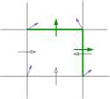
Figure 4: Intuition behind the construction of the rectangular abstraction transition system

There is one specific issue when considering the time progress of the abstracted trajectories. If there exists a point in a rectangle from which there is no trajectory diverging out through some exit face, then there is a self-transition defined for the rectangle. In particular, this situation signifies an equilibrium inside the rectangle. Such a rectangle is called non-transient. For affine systems there is known a sufficient and necessary condition that characterises non-transient rectangles by the vector field in the vertices of the rectangle. However, for the case of multi-affine system, only the necessary condition is known. Hence, for multi-affine systems BioDiVinE can treat as non-transient some states which are not necessarily non-transient.

      

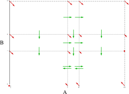
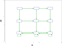
Figure 5: Example of a rectangular abstraction transition system

2.3 Model Checking

In the field of formal verification of software and hardware systems, model checking refers to the problem of automatically testing whether a simplified model of a system (a finite state automaton) meets a given specification. Specification is stated by means of a temporal logic formulae. In the setting of RATS, model checking can be used in two basic ways:

1. to automatically detect presence of particular dynamics phenomena in the system

2. to verify correctness of the model (i.e., checking whether some undesired property is exactly avoided)

In the case of dynamic systems we use Linear Temporal Logic (LTL) (see [11] for details on LTL syntax and semantics interpreted on automata). LTL can be also directly interpreted on trajectories of dynamic systems (see e.g. [14] for definition of the semantics). Given a dynamic system $S$ with a particular initial state we can then say that $S$ satisfies a formula $\varphi$, written $S\models\varphi$, only if the trajectory starting at the initial state satisfies $\varphi$. In the context of automata, LTL logic is interpreted universally provided that a formula $\varphi$ is satisfied by the automaton $A$, written $A\models\varphi$, only if each execution of the automaton starting from any initial state satisfies $\varphi$. The following theorem characterises the relation between validity of $\varphi$ in the rectangular abstraction automaton and in the original dynamic system.

Theorem 2.1

Consider a dynamic system $S$ and the associated RATS $A$. If $A\models\varphi$ then $S\models\varphi$.

The theorem states that when model checking of a particular property on a RATS returns true, we are sure that the property is satisfied in the original dynamic system. However, when the result is negative, the counterexample returned does not necessarily reflect any trajectory in the original system.

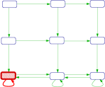
Figure 6: A counterexample contradicting the property of reaching $B>3$ in finite time

The system in Figure 5 satisfies a formula $\mathbf{F}\mathbf{G}(B\leq 3)$ expressing the temporal property stating that despite the choice of the initial state the system eventually stabilises at states where concentration of $B$ is kept below $3$. Now let us consider a formula $\mathbf{F}(B>3)$ expressing the property that despite the initial settings, the concentration of $B$ will eventually exceed the concentration level $3$. In this case the model checking returns one of the counterexamples as emphasised in Figure 6 stating that if initially $A<5$ and $B<3$ then $B$ is not increased while staying indefinitely long in the shaded state.

3 BioDiVinE Tool

BioDiVinE employs aggregate power of network-interconnected workstations (nodes) to analyse large-scale state transition systems whose exploration is beyond capabilities of sequential tools. System properties can be specified either directly in Linear Temporal Logic (LTL) or alternatively as processes describing undesired behaviour of systems under consideration (negative claim automata). From the algorithmic point of view, the tool implements a variety of novel parallel algorithms [10, 2] for cycle detection (LTL model checking). By these algorithms, the entire state space is uniformly split into partitions and every partition is distributed to a particular computing node. Each node is responsible for generating the respective state-space partition on-the-fly while storing visited states into the local memory.

The state space generator constructs the rectangular abstraction transition system for a given multi-affine system. The scheme of the tool architecture is provided in Figure 7. Library-level components are responsible for constructing, managing and distributing the state space. They form the core of the tool. The tool provides two graphical user interface components SpecAff — allowing editing of biological models in terms of chemical reactions, and SimAff — allowing visualisation of the simulation results.

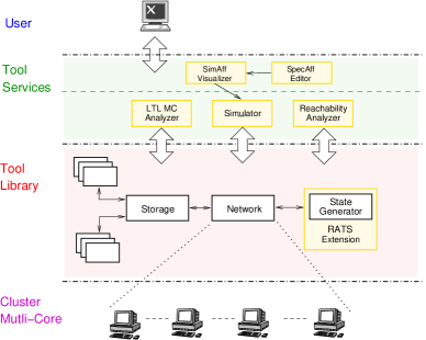
Figure 7: BioDiVinE Toolset Architecture

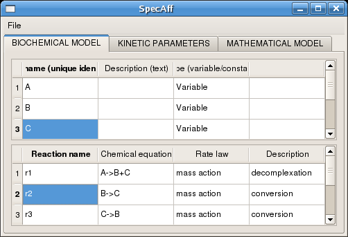
Figure 8: A biochemical model specified in BioDiVinE GUI

The input (biochemical) model is given by the following data:

• list of chemical species,

• list of partitioning thresholds given for each species,

• list of chemical reactions.

VARS:A,B,C

EQ:dA = (-0.1)*A
EQ:dB = 0.1*A + (-1)*B + 1*C
EQ:dC = 0.1*A + 1*B + (-1)*C

TRES:A: 0, 4, 6, 10
TRES:B: 0, 2, 10
TRES:C: 0, 2, 4, 10

INIT:   4:6, 0:2, 2:4

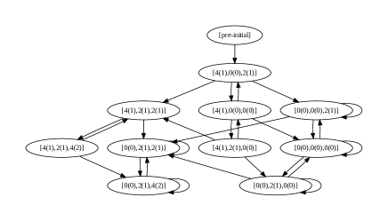
Figure 9: A multi-affine ODE model and its state space generated by BioDiVinE

The biochemical model together with the tested property and initial conditions are then automatically translated into a multi-affine system of ODEs forming the mathematical model that can be analysed by BioDiVinE algorithms. The mathematical model consists of the following data:

• list of variables,

• list of (multi-affine) ODEs,

• list of partitioning thresholds given for each species,

• list of initial rectangular subspaces (the union of these subspaces forms the initial condition),

• Büchi automaton representing an LTL property (this data is not needed for simulation).

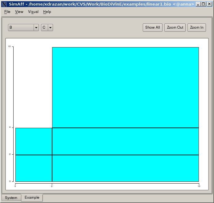
Figure 10: Visualisation of the state space in the BioDiVinE GUI, states are projected onto the BC concentration plane

An example of a simple three-species model representing three biochemical reactions $A\rightarrow B+C$, $B\rightleftharpoons C$ is showed in Figure 8. The first reaction is performed at rate $0.1~{}s^{-1}$. The second two reversible reactions are at rate $1~{}s^{-1}$. The respective mathematical model is showed in Figure 9 on the left in the textual .bio format. For each variable there is specified the equation as well as the list of real values representing individual threshold positions. The initial condition is defined in this particular case by a single rectangular subspace: $A\in\langle 4,6\rangle,B\in\langle 0,2\rangle$, and $C\in\langle 2,4\rangle$. The state space generated for this setting is depicted in Figure 9 on the right. Figure 10 demonstrates visualisation features of the BioDiVinE GUI.

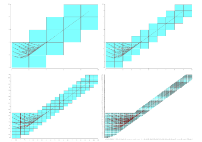
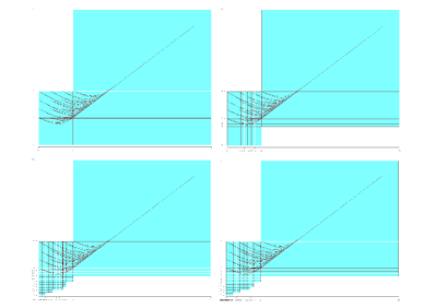
Figure 11: A visualisation of the state-spaces in BC projection with uniform (left) and automatic (right) gradual threshold refinement, manually augmented by numeric simulation trace from COPASI [12]

For model checking analysis, BioDiVinE relies on the parallel LTL model checking algorithms of the underlying DiVinE library [5]. A given LTL formula is translated into a Büchi automaton which represents its negation. That way the automaton represents the never claim property. The automaton is automatically generated for an LTL formula and merged with the mathematical model by the divine.combine utility. An example of a model extended with a never claim property is showed in Figure 12. In particular, the first automaton LTL_property1 specified in terms of the DiVinE language represents a never claim for the safety LTL formula $\mathbf{G}\neg(B\geq 4\wedge B\leq 4.5\wedge C\geq 3\wedge C\leq 3.5)$ expressing that concentrations of species $B$ and $C$ will never enter the specified rectangular region. The unreachability of a slightly different region is defined by the automaton for property 2. The results of the model-checking procedure are showed in Figure 13. Property 1 has been proved false by finding a run of the system visiting the specified region (states of run given as list), while property 2 has been proved true by extensively searching all the system runs and not finding any one that would cross the region specified in property 2.

VARS:A,B,C

EQ:dA = (-0.1)*A
EQ:dB = 0.1*A + (-1)*B + 1*C
EQ:dC = 0.1*A + (1)*B + (-1)*C

TRES:A: 0, 4, 6, 10
TRES:B: 0, 2, 10
TRES:C: 0, 2, 4, 10

INIT:   4:6, 0:2, 2:4

process LTL_property1 {
state q1, q2;
init q1;
accept q2;
trans
q1 -> q2 { guard B>4 && B<4.5
              && C>3 && C<3.5; },
q1 -> q1 {},
q2 -> q2 {};
}

system sync property LTL_property1;

process LTL_property2 {
state q1, q2;
init q1;
accept q2;
trans
q1 -> q2 { guard B>4 && B<4.5
              && C>5.5 && C<6; },
q1 -> q1 {},
q2 -> q2 {};
}

system sync property LTL_property2;

Figure 12: A multi-affine model extended with a never claim automaton for property 1 and property 2

The choice of threshold values for each variable affects greatly the shape and size of the generated state-space. The refinement of a given partitioning — the addition of more thresholds to a set of former thresholds — may result in the unreachability of a part of a region reachable before.

Since manual refinement of thresholds by adding numeric values can be tedious or unintuitive, two more advanced methods are available in BioDiVinE. The first method divides a given interval uniformly into subintervals of a given size, while the second method tries a more sophisticated automatic technique of dividing regions according to signs of the concentration derivatives inside these regions [18]. The state-spaces resulting from the gradual application of both threshold refinement approaches are depicted in Figure 11. It is important to mention that the overall size of the state-space depends exponentially on the number of thresholds for all species. However, in some cases the actual reachable subspace of the whole state-space may be only polynomial in the number of thresholds.

For any multi-affine model extended with a never claim automaton as showed in Figure 12, the parallel model checking algorithms can be directly called.

=======================
--- Accepting cycle ---
=======================
[pre-initial]
[4(1),0(0),2(1)-PP:0]
[4(1),2(1),2(1)-PP:0]
[4(1),2(1),3(2)-PP:0]
[4(1),4(2),3(2)-PP:1]
[0(0),4(2),3(2)-PP:1]
======= Cycle =======
[0(0),2(1),3(2)-PP:1]
[0(0),2(1),2(1)-PP:1]

==============================
  --- No accepting cycle ---
==============================
states:            33
transitions:       81
iterations:        1
size of a state:   16
size of appendix:  12
cross transitions: 0
all memory         56.5 MB
time:              0.115177 s
-------------------
0: local states:      33
0: local memory:      56.5

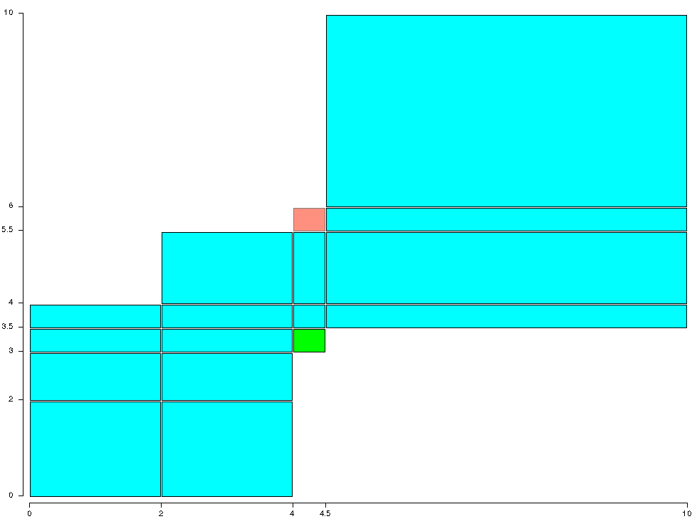
Figure 13: Results of model-checking for property 1 (left), property 2 (middle), visualisation of reachable (green) and unreachable (red) regions

We have performed several experiments [3] in order to show scaling of the algorithms when distributed on several cluster nodes. Figures 14 and 15 show scaling of model checking conducted on a simple model of a reaction network representing a catalytic reaction scaled for different numbers of intermediate products.

			Time on particular number of cluster processor cores (s)
$k$	States	Trans	1	4	8	12	16	20	24	28	32	36	40	44	48	52	56	60	64	68	72
5	$3\cdot 10^{4}$	$8.5\cdot 10^{4}$	15.4	4.9	2.7	1.8	1.4	$\bot$	$\bot$	$\bot$	$\bot$	$\bot$	$\bot$	$\bot$	$\bot$	$\bot$	$\bot$	$\bot$	$\bot$	$\bot$	$\bot$
	relative	speedup	1	3.14	5.7	8.56	11	$\bot$	$\bot$	$\bot$	$\bot$	$\bot$	$\bot$	$\bot$	$\bot$	$\bot$	$\bot$	$\bot$	$\bot$	$\bot$	$\bot$
10	$9\cdot 10^{5}$	$3.2\cdot 10^{6}$	$\top$	$\top$	$\top$	161	119	107	85	72	63	55	53	46	44	40	38	38	$\bot$	$\bot$	$\bot$
	relative	speedup	$\top$	$\top$	$\top$	1	1.35	1.5	1.89	2.24	2.56	2.93	3.04	3.5	3.66	4.03	4.24	4.24	$\bot$	$\bot$	$\bot$
15	$1.6\cdot 10^{6}$	$6.5\cdot 10^{6}$	$\top$	$\top$	$\top$	$\top$	$\top$	$\top$	$\top$	$\top$	222	204	177	156	146	129	122	117	110	98	93
	relative	speedup	$\top$	$\top$	$\top$	$\top$	$\top$	$\top$	$\top$	$\top$	1	1.09	1.25	1.42	1.52	1.72	1.82	1.9	2.02	2.27	2.39
20	$3.2\cdot 10^{6}$	$1.4\cdot 10^{7}$	$\top$	$\top$	$\top$	$\top$	$\top$	$\top$	$\top$	$\top$	$\top$	$\top$	$\top$	$\top$	$\top$	$\top$	$\top$	$\top$	202	180	173
	relative	speedup	$\top$	$\top$	$\top$	$\top$	$\top$	$\top$	$\top$	$\top$	$\top$	$\top$	$\top$	$\top$	$\top$	$\top$	$\top$	$\top$	1	1.12	1.17

Figure 14: Scaling of model checking algorithms on a homogeneous cluster

$$S+E\rightleftharpoons ES_{1}\rightleftharpoons ES_{2}\rightleftharpoons\cdots\rightleftharpoons ES_{k}\rightarrow P+E$$

$$\begin{array}[]{rcl}\dot{S}&=&ES_{1}-0.01\cdot E\cdot S\\ \dot{E}&=&ES_{1}-0.01\cdot S\cdot E+ES_{1}\\ \dot{ES_{1}}&=&0.01\cdot E\cdot S-ES_{1}-ES_{1}\\ \dot{ES_{2}}&=&\cdot ES_{1}-2\cdot ES_{2}+ES_{3}\\ &.&\\ &.&\\ &.&\\ \dot{ES}_{k-1}&=&ES_{k-2}-2\cdot ES_{k-1}+ES_{k}\\ \dot{ES}_{k}&=&ES_{k-1}-2\cdot ES_{k}\end{array}$$

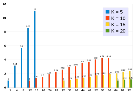
Figure 15: Scaling of model checking algorithms on a homogeneous cluster, X-axis shows number of cluster nodes, Y-axis gives speedup relative to system size and number of nodes

4 Case Study: Ammonium Transport in E. Coli

In this section we present a case study conducted using the current version of BioDiVinE. Since the rectangular abstraction method of multi-affine systems implemented in BioDiVinE is a relatively new result of applied control theory, its application is still in the stage of experimentation. In fact, we are still unaware of any case studies that apply this method to real biological models. In this case study we focus on demonstrating the usability of rectangular abstraction to analysis of biological models. To this end, we consider a simple biological model that specifies ammonium transport from external environment into the cells of Escherichia Coli. This simplified model is based on a published model of the E. Coli ammonium assimilation system [20] which was developed under the EC-MOAN project (http://www.ec-moan.org). The metabolic reactions and regulatory reactions in the original model were removed.

4.1 Model Description

E. coli can express membrane bound transport proteins for the transportion of small molecules from the environment into the cytoplasm at certain conditions. At normal ammonium concentration, the free diffusion of ammonia can provide enough flux for the growth requirement of nitrogen. When ammonium concentration is very low, E. coli cells express $AmtB$ (an ammonia transporter) to complement the deficient diffusion process. Three molecules of $AmtB$ (trimer) form a channel for the transportation of ammonium/ammonia. Protein structure analysis revealed that $AmtB$ binds $NH4^{+}$ at the entrance gate of the channel, deprotonates it and conducts $NH_{3}$ into the cytoplasm as illustrated in Figure 16 (left) [17]. At the periplasmic side of the channel there is a wider vestibule site capable of recruiting $NH_{4}^{+}$ cations. The recruited cations are passed through the hydrophobic channel where the pKa of $NH_{4}^{+}$ was shifted from $9.25$ to below $6$, thereby shifting the equilibrium toward the production of $NH_{3}$. $NH_{3}$ is finally released at the cytoplasmic gate and converted to $NH_{4}^{+}$ because intracellular pH ($7.5$) is far below the pKa of $NH_{4}^{+}$.

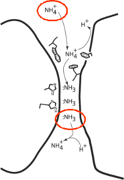
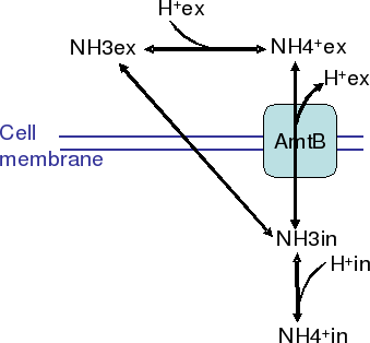
Figure 16: E. Coli ammonium transport mechanism and the respective pathway

In addition to the above mentioned $AmtB$ mediated transport, the bidirectional free diffusion of the uncharged ammonia through the membrane is also included in the simplified model. The intracellular $NH_{4}^{+}$ is then metabolised by Glutamine Synthetase (GS). The whole model is depicted in Figure 16 (right). The external ammonium is represented in the uncharged and charged forms denoted $NH_{3}ex$ and $NH_{4}^{+}ex$. Analogously, the internal ammonium forms are denoted $NH_{3}in$ and $NH_{4}^{+}in$. The biochemical model that combines $AmtB$ transport with $NH_{3}$ diffusion is given in Table 1. The kinetic parameters are based on the values in the original model.

$$\begin{array}[]{c@{\hspace{1cm}}l}AmtB+NH_{4}ex\stackrel{{\scriptstyle k_{1}}}{{\leftarrow}}\stackrel{{\scriptstyle k_{2}}}{{\rightarrow}}AmtB:NH_{4}\hfil\hskip 28.45274pt&k_{1}=5\cdot 10^{8},k_{2}=5\cdot 10^{3}\\ AmtB:NH_{4}\stackrel{{\scriptstyle k_{3}}}{{\rightarrow}}AmtB:NH_{3}+H_{ex}\hfil\hskip 28.45274pt&k_{3}=50\\ AmtB:NH_{3}\stackrel{{\scriptstyle k_{4}}}{{\rightarrow}}AmtB+NH_{3}in\hfil\hskip 28.45274pt&k_{4}=50\\ NH_{4}in\stackrel{{\scriptstyle k_{5}}}{{\rightarrow}}\hfil\hskip 28.45274pt&k_{5}=80\\ NH_{3}in+H_{in}\stackrel{{\scriptstyle k_{6}}}{{\leftarrow}}\stackrel{{\scriptstyle k_{7}}}{{\rightarrow}}NH_{4}in\hfil\hskip 28.45274pt&k_{6}=1\cdot 10^{15},k_{7}=5.62\cdot 10^{5}\\ NH_{3}ex\stackrel{{\scriptstyle k_{8}}}{{\leftarrow}}\stackrel{{\scriptstyle k_{9}}}{{\rightarrow}}NH_{3}in\hfil\hskip 28.45274pt&k_{8}=k_{9}=1.4\cdot 10^{4}\end{array}$$

Table 1: Biochemical model of ammonium transport

By employing the law of mass action kinetics the reaction network is transformed into the set of multi-affine ODEs as listed in Table 2. Since we are especially interested in how the concentrations of internal ammonium change with respect to the external ammonium concentrations, we employ the following simplifications:

• We do not consider the dynamics of the external ammonium forms, thus we take $NH_{3}ex$ and $NH_{4}^{+}ex$ as constants (the input parameters for the analysis).

• We assume constant intracellular pH ($7.5$) and extracellular pH ($7.0$), thus $H_{ex}$ and $H_{in}$ are calculated to be $3\cdot 10^{-8}$ and $10^{-7}$. Based on the extracellular pH and the total ammonium/ammonia concentration, concentrations of $NH_{3}ex$ and $NH_{4}^{+}ex$ can be calculated.

Without the loss of correctness, we simplify the notation of the cation $NH_{4}^{+}$ as $NH_{4}$.

$$\begin{array}[]{c}\frac{dAmtB}{dt}=-k_{1}\cdot AmtB\cdot NH_{4}ex+k_{2}\cdot AmtB:NH_{4}+k_{4}\cdot AmtB:NH_{3}\\ \frac{dAmtB:NH_{3}}{dt}=k_{3}\cdot AmtB:NH_{4}-k_{4}\cdot AmtB:NH_{3}\\ \frac{dAmtB:NH_{4}}{dt}=k_{1}\cdot AmtB\cdot NH_{4}ex-k_{2}\cdot AmtB:NH_{4}-k_{3}\cdot AmtB:NH_{4}\\ \frac{dNH_{3}in}{dt}=k_{4}\cdot AmtB:NH_{3}-k_{7}\cdot NH_{3}in+k_{6}\cdot NH_{4}in\\ \frac{dNH_{4}in}{dt}=k_{5}\cdot NH_{4}in+k_{7}\cdot NH_{3}in\cdot H_{in}-k_{6}\cdot NH_{4}in\\ \end{array}$$

Table 2: Mathematical model of ammonium transport

4.2 Model Analysis

From the essence of biophysical laws, it is clear that the maximal reachable concentration level accumulated in the internal ammonium forms directly depends on the ammonium sources available in the environment. However, it is not directly clear what particular maximal level of internal ammonium is achievable at given amount of external ammonium (distributed into the two forms). In the analysis we have focused on just this phenomenon. More precisely, the problem to solve has been to analyse how the setting of the model parameters $NH_{3}ex$ and $NH_{4}^{+}ex$ affects the maximal concentration level of $NH_{3}in$ and $NH_{4}^{+}in$ reachable from given initial conditions.

During discussions with biologists we have found out that there is currently not available any in vitro measurement of the $AmtB$-concentration (and also the concentrations of dimers $AmtB:NH_{3}$ and $AmtB:NH_{4}$). Hence there has appeared the need to analyse the model with uncertain initial conditions. Such a setting fits the current features of BioDiVinE, especially the rectangular abstraction that naturally abstracts away the exact concentration values up to the intervals between certain concentration levels.

4.2.1 Maximal reachable levels of internal ammonium forms

At first, we have considered the (abstracted) initial condition to be set to the following intervals between concentration values:

$$AmtB\in\langle 0,1\cdot 10^{-5}\rangle,\quad AmtB:NH_{3}\in\langle 0,1\cdot 10^{-5}\rangle,\quad AmtB:NH_{4}\in\langle 0,1\cdot 10^{-5}\rangle,$$

$$NH_{3}in\in\langle 1\cdot 1^{-6},1.1\cdot 10^{-6}\rangle,\quad NH_{4}in\in\langle 2\cdot 10^{-6},2.1\cdot 10^{-6}\rangle$$

Note that the upper bounds as well as the initial intervals of internal ammonium forms have been set with respect to the available data obtained from the literature.

We have considered two rectangular partitions. The partition $(1)$ has been set basically according to the initial conditions. The partition $(2)$ has been obtained by running one iteration of the automatic threshold refinement procedure to partition $(1)$. Numbers of thresholds per each variable are given in Table 3.

Partition	$AmtB$	$AmtB:NH_{3}$	$AmtB:NH_{4}$	$NH_{3}in$	$NH_{4}in$
$(1)$	$7$	$3$	$3$	$6$	$4$
$(2)$	$7$	$9$	$3$	$8$	$26$

Table 3: Numbers of thresholds in partitions $(1)$ and $(2)$

We have conducted several model checking experiments in order to determine the maximal reachable concentration levels of $NH_{3}in$ and $NH_{4}^{+}in$. In particular, we have searched for the lowest $\alpha$ satisfying the property $\mathbf{G}(NH_{3}in<\alpha)$ and the lowest $\beta$ satisfying $\mathbf{G}(NH_{4}in<\beta)$. The property $\mathbf{G}p$ requires that all paths available in the rectangular abstraction from the states specified by the initial condition must satisfy the given proposition $p$ at every state. Note that if the model checking method finds the property $\mathbf{G}p$ false in the model, it also returns a counterexample for that. The counterexample satisfies the negation of the checked formula, which is in this case $\mathbf{F}\neg p$. Interpreting this observation intuitively for the given formulae, we use model checking to find a path on which the species $NH_{3}in$ (resp. $NH_{4}in$) exceeds the level $\alpha$ (resp. $\beta$).

We did not want to get precise values of $\alpha,\beta$, but we rather wanted to get their good approximation. At the starting point, we substituted for $\alpha$ (resp. $\beta$) the upper initial bounds of the respective variables. Then we found the requested values by iteratively increasing and decreasing $\alpha$ (resp. $\beta$). The obtained results are summarised in Table 4.

Partition $(1)$				Partition $(2)$
$\alpha$	$\mathbf{G}(NH_{3}in<\alpha)$	$\#$ states	Time ($\#$ nodes)	$\mathbf{G}(NH_{3}in<\alpha)$	$\#$ states	Time ($\#$ nodes)
$1.1\cdot 10^{-6}$	true	1081	0.36 s (1)	true	$1.5\cdot 10^{5}$	1.9 s (18)
$\beta$	$\mathbf{G}(NH_{4}in<\beta)$	$\#$ states	Time ($\#$ nodes)	$\mathbf{G}(NH_{4}in<\beta)$	$\#$ states	Time ($\#$ nodes)
$1\cdot 10^{-3}$	true	2161	0.45 s (1)	true	$1.6\cdot 10^{5}$	2 s (18)
$5\cdot 10^{-4}$	false	4753	1.9 s (1)	false	$2.7\cdot 10^{5}$	3 s (18)
$6\cdot 10^{-4}$	true	2161	0.43 s (1)	true	$1.5\cdot 10^{5}$	1.8 s (18)
$5.4\cdot 10^{-4}$	true	1441	0.27 s (1)	true	$2.1\cdot 10^{5}$	4.2 s (18)
$5.3\cdot 10^{-4}$	false	3421	1.2 s (1)	false	$2.7\cdot 10^{5}$	2.2 s (18)

Table 4: Experiments on detecting maximal reachable levels of internal ammonium forms

The results have shown that $NH_{3}in$ does not exceed its initial level no matter how the external ammonium is distributed between $NH_{3}ex$ and $NH_{4}^{+}ex$. The upper bound concentration considered for both $NH_{3}ex$ and $NH4^{+}ex$ has been set to $1\cdot 10^{-5}$ which goes with the typical level of concentration of the gas in the environment.

In the case of $NH_{4}in$ we have found that the upper bound to maximal reachable level is in the interval $\beta\in\langle 5.3\cdot 10^{-4},5.4\cdot 10^{-4}\rangle$. Since the counterexample achieved can be a spurious one due to the overapproximating abstraction, the exact maximal reachable value may be lower. To this end we have conducted several numerical simulations which give us the argument that our estimation of $\beta$ is plausible.

4.2.2 Dependence of stable internal ammonium on changes in external conditions

In the second experiment, we have focused on determining how much external ammonium have to be increased in particular form in order to stimulate $NH3in$ to exceed the considered initial level. The setting of partitions and initial conditions has been considered the same as in the previous experiments.

First, we have varied the constant amount of $NH_{3}ex$ to find at which level of $NH_{3}ex$ the maximal reachable level of $NH_{3}in$ is affected. More precisely, we have observed for which setting of $NH_{3}ex$ the property $\varphi\equiv\mathbf{G}(NH_{3}in<1.1\cdot 10^{-6})$ is true and for which it is not. The relevant experiments are summarised in Table 5. We have found out that if $NH_{3}ex$ is set to $19.6\cdot 10^{-4}$ or higher level then $NH_{3}in$ increases above the upper initial bound $1.1\cdot 10^{-6}$. The counterexamples returned again agree with numerical simulations.

Partition $(1)$				Partition $(2)$
$NH_{3}ex$	$\varphi$	$\#$ states	Time ($\#$ nodes)	$\varphi$	$\#$ states	Time ($\#$ nodes)
$19.5\cdot 10^{-4}$	true	901	0.22 s (1)	true	$1.4\cdot 10^{5}$	1.9 s (36)
$19.6\cdot 10^{-4}$	false	1261	0.6 s (1)	false	$3.4\cdot 10^{5}$	5.9 s (36)

Table 5: Experiments on detecting $NH_{3}ex$ levels affecting maximal reachable $NH_{3}in$

Finally, we have varied the amount of $NH_{4}^{+}ex$ in order to find at which level of $NH_{4}^{+}ex$ the maximal reachable level of $NH_{3}in$ is affected. The results presented in Table 6 give us the conclusion that despite the level of $NH_{4}^{+}ex$ (checked up to $10^{12}$), the maximal level reached by $NH_{3}in$ remains the same. In particular, $NH_{3}in$ does not exceed the initial bounds.

Partition $(1)$
$NH_{4}ex$	$\varphi$	$\#$ states	Time ($\#$ nodes)
$1$	true	901	0.25 s (1)
$1\cdot 10^{12}$	true	901	0.25 s (1)

Table 6: Experiments on detecting $NH_{4}^{+}ex$ levels affecting maximal reachable $NH_{3}in$

4.2.3 Performance

All the experiments have been performed on a homogeneous cluster allowing computation on up-to 22 nodes each equipped with 16GB of RAM and a quad-core processor Intel Xeon 2GHz. The model we have dealt with contained $5$ dynamic variables and $2$ constants. With partition $(1)$ the generated state space had maximally $4753$ states and with partition $(2)$ maximally $3.4\cdot 10^{5}$. When trying to run one more step of automatic partition refinement, the number of thresholds exceeded the memory reserved for storing of the mathematical model. Note that the model has to be stored in the memory of each node. Only the state space is distributed over the cluster.

5 Conclusion

In this paper, we have presented the current version of BioDiVinE tool which implements rectangular abstraction of continuous models of biochemical reaction systems. The tool provides the framework for specification and analysis of biochemical systems. The supported analysis technique is based on the model checking method. Linear temporal logic is used for encoding of the properties to be observed on abstracted systems.

The tool provides parallel model checking algorithms that allow fast response times of the analysis. We have provided a case study on which the key features of the tool are demonstrated. The case study has showed that the tool can be used for quickly getting the approximation of maximal reachable concentration levels of individual species in the model. In general, we have analysed the model with respect to the set of safety properties which are technically tackled by construction of the state space reachable from the given initial states. We have found out that the main advantage of the rectangular abstraction is the possibility to analyse the system with uncertain initial conditions.

The current drawback of the abstraction method is strong overapproximation of non-transient states in multi-affine systems. In consequence, analysis of liveness kind of properties (e.g., oscillations, instability) is infeasible because of large amount of spurious counterexamples that come from false identification of non-transient states. However, this is not the case for affine systems on which liveness properties can be checked without these problems. Since the analysed systems are typically non-affine, we can still employ the liveness checking on their linearised approximations. However, by the linearisation process the precision of the analysis is significantly reduced. Improving the tool in these aspects requires further research.

In general, we leave for future work the development of methods for identification of spurious paths. We think that one of the promising directions in using the discrete abstractions for analysis of biological models is employing the model-checking-based analysis for extensive exploration of properties. In particular, instead of returning only one path, the model checker should provide a set of paths. In this directions we aim to continue the research.

References

- [1]
- [2] J. Barnat, L. Brim & J. Chaloupka (2005): From Distributed Memory Cycle Detection to Parallel LTL Model Checking. Electronic Notes in Theoretical Computer Science 133(1), pp. 21–39.
- [3] J. Barnat, L. Brim, I. Černá, S. Dražan, J. Fabriková & D. Šafránek (2009): Computational Analysis of Large-Scale Multi-Affine ODE Models Accepted to High Performance Computational Systems Biology (HIBI) 2009.
- [4] J. Barnat, L. Brim, I. Černá, S. Dražan, J. Fabriková & D. Šafránek (2009): On Algorithmic Analysis of Transcriptional Regulation by LTL Model Checking. Theoretical Computer Science 410, pp. 3128–3148.
- [5] J. Barnat, L. Brim, I. Černá, P. Moravec, P. Ročkai & P. Šimeček (2006): DiVinE – A Tool for Distributed Verification (Tool Paper). In: Computer Aided Verification, LNCS 4144/2006. Springer, pp. 278–281.
- [6] G. Batt, C. Belta & R. Weiss (2007): Model checking liveness properties of genetic regulatory networks. In: Conference on Tools and Algorithms for the Construction and Analysis of Systems, LNCS 4424. Springer, pp. 323–338.
- [7] G. Batt, C. Belta & R. Weiss (2008): Model checking genetic regulatory networks with parameter uncertainty. IEEE Transactions on Circuits and Systems and IEEE Transactions on Automatic Control, Special Issue on Systems Biology , pp. 215–229.
- [8] C. Belta & L.C.G.J.M. Habets (2006): Controlling a class of nonlinear systems on rectangles. IEEE Transactions on Automatic Control 51(11), pp. 1749–1759.
- [9] L. Calzone, F. Fages & S. Soliman (2006): BIOCHAM: an environment for modeling biological systems and formalizing experimental knowledge. Bioinformatics 22(14), pp. 1805–1807.
- [10] I. Černá & R. Pelánek (2003): Distributed Explicit Fair Cycle Detection (Set Based Approach). In: Model Checking Software. 10th International SPIN Workshop, LNCS 2648. Springer, pp. 49 – 73.
- [11] E.M. Clarke, O. Grumberg & D.A. Peled (2000): Model Checking. MIT Press.
- [12] S. Hoopes et.al. (2006): COPASI – a COmplex PAthway SImulator. Bioinformatics 22, pp. 3067–74.
- [13] M. Feinberg (1987): Chemical reaction network structure and the stability of complex isothermal reactors I. The deficiency zero and the deficiency one theorems. Chemical Engineering Science 42, pp. 2229–2268.
- [14] S.K. Jha, E.M. Clarke, C.J. Langmead, A. Legay, A. Platzer & A.P. Zuliani (2009): A Bayesian Approach to Model Checking Biological Systems. In: Proc. of Computational Methods in Systems Biology (CMSB 2009), 5688. Springer, pp. 218–234.
- [15] H. de Jong, J. Geiselmann, C. Hernandez & M. Page (2003): Genetic Network Analyzer: qualitative simulation of genetic regulatory networks. Bioinformatics 19(3), pp. 336–344. Available at http://www-helix.inrialpes.fr/gna.
- [16] H. de Jong, J.L. Gouzé, C. Hernandez, M. Page, T. Sari & J. Geiselmann (2004): Qualitative simulation of genetic regulatory networks using piece-wise linear models. Bull. Math. Biology 66, pp. 301–340.
- [17] S. Khademi, J. O’Connell III, J. Remis, Y. Robles-Colmenares, L.J. Miercke & R.M. Stroud (2004): Mechanism of ammonia transport by Amt/MEP/Rh: Structure of AmtB at 1.35. Science 305(5690), pp. 1587–1594.
- [18] M. Kloetzer & C. Belta (2008): Reachability analysis of multi-affine systems. Transactions of the Institute of Measurement and Control In press.
- [19] X. Liu, J. Jiang, O. Ajayi, X. Gu, D. Gilbert & R. Sinnott (2008): BioNessie. Global Healthgrid: e-Science Meets Biomedical Informatics - Proceedings of HealthGrid 2008 138, pp. 147–157.
- [20] H. Ma, F. Boogerd & I. Goryanin (2009): Modelling nitrogen assimilation of Escherichia coli at low ammonium concentration. Journal of Biotechnology Doi:10.1016/j.jbiotec.2009.09.003.