On spectral stability of solitary waves of nonlinear Dirac equation on a line

Abstract

We study the spectral stability of solitary wave solutions to the nonlinear Dirac equation in one dimension. We focus on the Dirac equation with cubic nonlinearity, known as the Soler model in (1+1) dimensions and also as the massive Gross-Neveu model. Presented numerical computations of the spectrum of linearization at a solitary wave show that the solitary waves are spectrally stable. We corroborate our results by finding explicit expressions for several of the eigenfunctions. Some of the analytic results hold for the nonlinear Dirac equation with generic nonlinearity.

1 Introduction

The study of stability of localized solutions to nonlinear dispersive equations takes its origin in [Der64], where the instability of stationary localized solutions to nonlinear Klein-Gordon equation was proved. It was suggested there that quasistationary finite energy solutions of the form $\phi(x)e^{-i\omega t}$, which we call solitary waves, could be stable. The first results on (spectral) stability of the linearization at solitary wave solutions to a nonlinear Schrödinger equation were obtained in [Zak67, VK73]. Orbital stability and instability of solitary waves in nonlinear Schrödinger and Klein-Gordon equations have been extensively studied in [Sha83, SS85, Sha85, Wei86, GSS87]. The asymptotic stability of solitary waves in nonlinear Schrödinger equation was proved in certain cases in [Wei85, BP93, SW92, SW99, Cuc01, BS03, CM08].

Systems with Hamiltonians that are not sign-definite are notoriously difficult, due to the absence of the a priori bounds on the Sobolev norm. Important examples of such systems are the Dirac-Maxwell system [Gro66] and the nonlinear Dirac equation [Sol70], which have been receiving a lot of attention in theoretical physics in relation to classical models of elementary particles. The stability of solitary wave solutions to the nonlinear Dirac equation is far from being understood. Some partial results on the numerical analysis of spectral stability of solitary waves are contained in [Chu07]. Generalizing the results on orbital stability of solitary waves [GSS87] to the nonlinear Dirac equation does not seem realistic, because of the corresponding energy functional being sign-indefinite; instead, one hopes to prove the asymptotic stability, using linear stability combined with the dispersive estimates. The first results on asymptotic stability for the nonlinear Dirac equation are already appearing [PS10, BC11], with the assumptions on the spectrum of the linearized equation playing a crucial role. In view of these applications, the spectrum of the linearization at a solitary wave is of great interest.

In the present paper, we give numerical and analytical justifications of spectral stability of small amplitude solitary wave solutions to the nonlinear Dirac equation in one dimension.

Let us remind the terminology. Given a solitary wave $\phi(x)e^{-i\omega t}$, we consider a small perturbation of the form $\psi(x,t)=(\phi(x)+\rho(x,t))e^{-i\omega t}$. We call a solitary wave $\phi(x)e^{-i\omega t}$ linearly unstable if the equation on $A$ is given by $\partial_{t}\rho=A\rho+o(\rho)$, with $A$ having eigenvalues with positive real part. If the entire spectrum of $A$ is on the imaginary axis, we call the solitary wave spectrally stable. The solitary wave is called orbitally stable [GSS87] if any solution $\psi(t)$ initially close to $\phi$ (in a certain norm, usually the energy norm) will exist globally, remaining close to the orbit spanned by $\phi$ for all times:

For any $\epsilon>0$ there is $\delta>0$ such that if $\|\psi_{0}-\phi\|<\delta$, then there is a solution $\psi(t)$

which exists for all $t\geq 0$ and satisfies $\psi|_{{}_{t=0}}=\psi_{0}$,  $\sup\limits_{t\geq 0}\inf\limits_{s\in\mathbb{R}}\|\psi|_{{}_{t}}-e^{is}\phi\|<\epsilon$.

Otherwise, the solitary wave is called orbitally unstable. A solitary wave is called asymptotically stable if any solution initially close to it (in a certain norm) will converge (in a certain norm) to this or to a nearby solitary wave. Linear instability of solitary waves generically leads to orbital instability [Gri88, GO10]; at the same time, spectral stability does not imply neither orbital nor asymptotic stability.

ACKNOWLEDGMENTS The authors would like to thank Marina Chugunova for providing us with her preliminary numerical results on spectral properties of coupled mode equations (see also [Chu07]) which greatly stimulated our research. The authors are grateful to Nabile Boussaid, Thomas Chen, Linh Nguyen, Dmitry Pelinovsky, Bjorn Sandstede, Walter Strauss, Boris Vainberg, and Michael Weinstein for most helpful discussions.

2 Nonlinear Dirac equation

The nonlinear Dirac equation has the form

$$i\partial_{t}\psi=-i\sum_{j=1}^{n}\alpha_{j}\partial_{x_{j}}\psi+\beta g(\psi^{\ast}\beta\psi)\psi,\qquad\psi(x,t)\in\mathbb{C}^{N},\qquad x\in\mathbb{R}^{n},$$ (2.1)

with $\psi^{\ast}$ being the Hermitian conjugate of $\psi$. The Hermitian matrices $\alpha_{j}$ and $\beta$ are chosen so that

$$\alpha_{j}^{2}=I,\qquad\beta^{2}=I,\qquad\{\alpha_{j},\alpha_{k}\}=2\delta_{jk},\qquad\{\alpha_{j},\beta\}=0,\qquad 1\leq j,\,k\leq n.$$

We assume that the nonlinearity $g$ is smooth and real-valued. We denote $m\equiv g(0)$. Equation (2.1) with $n=3$ and $g(s)=1-s$ is known as the Soler model [Sol70] (when $n=3$, one can take Dirac spinors with $N=4$ components). The case $n=1$ (when one can take spinors with $N=2$ components) is known as the massive Gross-Neveu model [GN74, LG75].

In the present paper, we consider the Dirac equation in $\mathbb{R}^{1}$:

$$i(\partial_{t}+\alpha\partial_{x})\psi=g(\psi^{\ast}\beta\psi)\beta\psi,\qquad\psi(x,t)\in\mathbb{C}^{2},\qquad x\in\mathbb{R}^{1}.$$ (2.2)

As $\alpha$ and $\beta$, we choose

$$\alpha=-\sigma_{2},\qquad\beta=\sigma_{3},$$ (2.3)

with the Pauli matrices $\sigma_{1}=\left(\begin{matrix}0&1\\ 1&0\end{matrix}\right),$ $\sigma_{2}=\left(\begin{matrix}0&-i\\ i&0\end{matrix}\right),$ $\sigma_{3}=\left(\begin{matrix}1&0\\ 0&-1\end{matrix}\right).$ Noting that $\psi^{\ast}\sigma_{3}\psi=|\psi_{1}|^{2}-|\psi_{2}|^{2}$, we rewrite equation (2.2) as the following system:

$$\left\{\begin{array}[]{ll}i\partial_{t}\psi_{1}=\partial_{x}\psi_{2}+g(|\psi_{1}|^{2}-|\psi_{2}|^{2})\psi_{1},\\ i\partial_{t}\psi_{2}=-\partial_{x}\psi_{1}-g(|\psi_{1}|^{2}-|\psi_{2}|^{2})\psi_{2}.\end{array}\right.$$ (2.4)

3 Solitary wave solutions

We start by demonstrating the existence of solitary wave solutions and exploring their properties.

Definition 3.1.

The solitary waves are solutions to (2.1) of the form

$$\psi(x,t)=\phi_{\omega}(x)e^{-i\omega t},\qquad\phi_{\omega}\in H^{1}(\mathbb{R}^{n},\mathbb{C}^{N}),\ \omega\in\mathbb{R}.$$

The following result follows from [CV86].

Lemma 3.2.

Assume that

$$m:=g(0)>0.$$ (3.1)

Let $G(s)$ be the antiderivative of $g(s)$ such that $G(0)=0$. Assume that for given $\omega\in\mathbb{R}$, $0<\omega<m$, there exists $\mathscr{X}_{\omega}>0$ such that

$$\omega\mathscr{X}_{\omega}=G(\mathscr{X}_{\omega}),\qquad\omega\neq g(\mathscr{X}_{\omega}),\qquad\mbox{and}\qquad\omega s<G(s)\quad{\rm for}\ s\in(0,\mathscr{X}_{\omega}).$$ (3.2)

Then there is a solitary wave solution $\psi(x,t)=\phi_{\omega}(x)e^{-i\omega t}$, where

$$\phi_{\omega}(x)=\left[\begin{matrix}v(x)\\ u(x)\end{matrix}\right],\qquad v,\ u\in H^{1}(\mathbb{R}),$$ (3.3)

with both $v$ and $u$ real-valued, $v$ being even and $u$ odd.

More precisely, let us define $\mathscr{X}(x)$ and $\mathscr{Y}(x)$ by

$$\mathscr{X}=v^{2}-u^{2},\qquad\mathscr{Y}=vu.$$ (3.4)

Then $\mathscr{X}(x)$ is the solution to

$$\mathscr{X}^{\prime\prime}=-\partial_{\mathscr{X}}(-2G(\mathscr{X})^{2}+2\omega^{2}\mathscr{X}^{2}),\qquad\mathscr{X}(0)=\mathscr{X}_{\omega},\qquad\mathscr{X}^{\prime}(0)=0,$$ (3.5)

and $\mathscr{Y}(x)=-\frac{1}{4\omega}\mathscr{X}^{\prime}(x)$.

Proof.

From (2.4), we obtain:

$$\left\{\begin{array}[]{ll}\omega v=\partial_{x}u+g(|v|^{2}-|u|^{2})v,\\ \omega u=-\partial_{x}v-g(|v|^{2}-|u|^{2})u.\end{array}\right.$$ (3.6)

Assuming that both $v$ and $u$ are real-valued (this will be justified once we found real-valued $v$ and $u$), we can rewrite (3.6) as the following Hamiltonian system, with $x$ playing the role of time:

$$\left\{\begin{array}[]{ll}\partial_{x}u=\omega v-g(v^{2}-u^{2})v=\partial_{v}h(v,u),\\ -\partial_{x}v=\omega u+g(v^{2}-u^{2})u=\partial_{u}h(v,u),\end{array}\right.$$ (3.7)

where the Hamiltonian $h(v,u)$ is given by

$$h(v,u)=\frac{\omega}{2}(v^{2}+u^{2})-\frac{1}{2}G(v^{2}-u^{2}).$$ (3.8)

The solitary wave corresponds to a trajectory of this Hamiltonian system such that

$$\lim\limits_{x\to\pm\infty}v(x)=\lim\limits_{x\to\pm\infty}u(x)=0,$$

hence $\lim\limits_{x\to\pm\infty}\mathscr{X}=0$. Since $G(s)$ satisfies $G(0)=0$, we conclude that

$$h(v(x),u(x))\equiv 0,$$ (3.9)

which leads to

$$\omega(v^{2}+u^{2})=G(v^{2}-u^{2}).$$ (3.10)

Studying the level curves which solve this equation is most convenient in the coordinates

$$\mathscr{X}=v^{2}-u^{2},\qquad\mathscr{Z}=v^{2}+u^{2};$$

see Figure 1. We conclude from (3.10) and Figure 1 that solitary waves may correspond to $|\omega|<m$, $\omega\neq 0$.

Remark 3.3.

If $\omega>0$, then there are solitary waves such that $v$ is nonzero while $u$ changes its sign (shifting the origin, we may assume that this happens at $x=0$). For $\omega<0$, there are solitary waves such that $u\neq 0$, while $v$ changes its sign.

Remark 3.4.

In the case when $G(s)$ is odd, for each solitary wave corresponding to $\omega\in\mathbb{R}$ there is a solitary wave corresponding to $-\omega$. More precisely, in this case, if $\left[\begin{matrix}v(x)\\ u(x)\end{matrix}\right]e^{-i\omega t}$ is a solitary wave, then so is $\left[\begin{matrix}u(x)\\ v(x)\end{matrix}\right]e^{i\omega t}$.

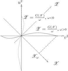
Figure 1: Existence of solitary waves in the coordinates $\mathscr{X}=v^{2}-u^{2}$, $\mathscr{Z}=v^{2}+u^{2}$. Solitons with $\omega>0$ and $\omega<0$ correspond to the bump on the $v^{2}$ axis and to the dotted bump on the $u^{2}$ axis (respectively) in the first quadrant.

The functions $\mathscr{X}(x)$ and $\mathscr{Y}(x)$ introduced in (3.4) are to solve

$$\left\{\begin{array}[]{ll}\mathscr{X}^{\prime}=-4\omega\mathscr{Y},\\ \mathscr{Y}^{\prime}=-(v^{2}+u^{2})g(\mathscr{X})+\omega\mathscr{X}=-\frac{1}{\omega}G(\mathscr{X})g(\mathscr{X})+\omega\mathscr{X},\end{array}\right.$$ (3.11)

and to have the asymptotic behavior $\lim_{|x|\to\infty}\mathscr{X}(x)=0$, $\lim_{|x|\to\infty}\mathscr{Y}(x)=0$. In the second equation in (3.11), we used the relation (3.10). The system (3.11) can be written as the following equation on $\mathscr{X}$:

$$\mathscr{X}^{\prime\prime}=-\partial_{\mathscr{X}}(-2G(\mathscr{X})^{2}+2\omega^{2}\mathscr{X}^{2}).$$ (3.12)

This equation describes a particle in the potential $V_{\omega}(s)=-2G(s)^{2}+2\omega^{2}s^{2}$; see Figure 2. Due to the energy conservation (with $x$ playing the role of time), we get:

$$\frac{\mathscr{X}^{\prime 2}}{2}-2G(\mathscr{X})^{2}+2\omega^{2}\mathscr{X}^{2}=\frac{\mathscr{X}^{\prime 2}}{2}+V_{\omega}(\mathscr{X})=0.$$ (3.13)

Using the expression for $\mathscr{X}^{\prime}$ from (3.11), relation (3.13) could be rewritten as

$$0=\frac{\mathscr{X}^{\prime 2}}{2}+V_{\omega}(\mathscr{X})=8\omega^{2}\mathscr{Y}^{2}-2G(\mathscr{X})^{2}+2\omega^{2}\mathscr{X}^{2}=2\omega^{2}\big{(}4v^{2}u^{2}+(v^{2}-u^{2})^{2}\big{)}-2G^{2},$$ (3.14)

which follows from (3.10).

For a particular value of $\omega$, there will be a positive solution $\mathscr{X}(x)$ such that $\lim_{x\to\pm\infty}\mathscr{X}(x)=0$ if there exists $\mathscr{X}_{\omega}>0$ so that (3.2) is satisfied (see Figure 2). We shift $x$ so that $\mathscr{X}$ so that $\mathscr{X}(0)=\mathscr{X}_{\omega}$; then $\mathscr{X}(x)$ is an even function.

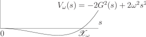
Figure 2: Effective potential $V_{\omega}(s)$. A solitary wave corresponds to a trajectory which satisfies $\mathscr{X}(0)=\mathscr{X}_{\omega}$, $\lim_{|x|\to\infty}\mathscr{X}(x)=0$.

Once $\mathscr{X}(x)$ is known, $\mathscr{Y}(x)$ is obtained from (3.11), and then we can express $v(x)$, $u(x)$. ∎

Remark 3.5.

Note that for $0<|\omega|<1$, the functions $v(x)$ and $u(x)$ are exponentially decaying as $|x|\to\infty$. Indeed, the exponential decay of $\mathscr{X}(x)$ could be deduced from (3.12). Then the exponential decay of $\mathscr{Z}(x)=v(x)^{2}+u(x)^{2}$ follows from the relation $\mathscr{Z}=G(\mathscr{X})/\omega$ (Cf. (3.10)).

3.1 Explicit solitary waves in a particular case

As shown in [LG75] for the massive Gross-Neveu model (the Soler model in 1D), in the special case of the potential

$$G(s)=s-\frac{s^{2}}{2},$$ (3.15)

the solitary waves can be found explicitly. Substituting $G(s)$ from (3.15) into (3.13), we get the following relation:

$$dx=-\frac{d\mathscr{X}}{2\sqrt{(\mathscr{X}-\mathscr{X}^{2}/2)^{2}-\omega^{2}\mathscr{X}^{2}}}=-\frac{d\mathscr{X}}{2\mathscr{X}\sqrt{(1-\mathscr{X}/2)^{2}-\omega^{2}}}.$$ (3.16)

We use the substitution

$$1-\frac{\mathscr{X}}{2}=\frac{\omega}{\cos{2\Theta}},\qquad\mathscr{X}=2\Big{(}1-\frac{\omega}{\cos{2\Theta}}\Big{)}.$$ (3.17)

Then

$$dx=-\frac{d\mathscr{X}}{2\mathscr{X}\sqrt{(1-\mathscr{X}/2)^{2}-\omega^{2}}}=\frac{2\frac{2\omega\sin 2\Theta}{\cos^{2}{2\Theta}}\,d\Theta}{4(1-\frac{\omega}{\cos{2\Theta}})\sqrt{\frac{\omega^{2}}{\cos^{2}2\Theta}-\omega^{2}}}=\frac{d\Theta}{\cos{2\Theta}-\omega},$$ (3.18)

$$x=\frac{1}{2\kappa}\ln\biggr{|}\frac{\sqrt{\mu}+\tan\Theta}{\sqrt{\mu}-\tan\Theta}\biggr{|},$$ (3.19)

where

$$\kappa=\sqrt{1-\omega^{2}},\qquad\mu=\frac{1-\omega}{1+\omega}.$$ (3.20)

Then

$$(\sqrt{\mu}+\tan\Theta)e^{2\kappa x}=\sqrt{\mu}-\tan\Theta,\qquad\tan\Theta(x)=-\sqrt{\mu}\tanh{\kappa x}.$$ (3.21)

Also note that

$$\mathscr{X}(x)=2\left(1-\frac{\omega}{\cos 2\Theta}\right)=2\left(1-\frac{\omega}{2\cos^{2}\Theta-1}\right)=2\left(1-\omega\frac{1+\tan^{2}\Theta(x)}{1-\tan^{2}\Theta(x)}\right),$$ (3.22)

and then

$$\mathscr{Y}(x)=-\frac{1}{4\omega}\mathscr{X}^{\prime}(x)=-\frac{1}{4}\frac{2}{\cos^{2}2\Theta}(-2\sin 2\Theta)\frac{d\Theta}{dx}$$

$$=-\frac{1}{4}\frac{2}{\cos^{2}2\Theta}(-2\sin 2\Theta)(\cos 2\Theta-\omega)=\frac{\mathscr{X}}{2}\tan 2\Theta$$

$$=\frac{\mathscr{X}}{2}\frac{2\tan\Theta}{1-\tan^{2}\Theta}=-\mathscr{X}(x)\frac{\sqrt{\mu}\tanh\kappa x}{1-\mu\tanh^{2}\kappa x}.$$

Denote

$$\mathscr{Z}(x)=v^{2}(x)+u^{2}(x).$$ (3.23)

Then

$$\mathscr{Z}(x)=\frac{2}{\cos 2\Theta(x)}\left(1-\frac{\omega}{\cos 2\Theta(x)}\right)=2\frac{1+\tan^{2}\Theta(x)}{1-\tan^{2}\Theta(x)}\left(1-\omega\frac{1+\tan^{2}\Theta(x)}{1-\tan^{2}\Theta(x)}\right).$$

The other functions are expressed from $\mathscr{Z}$ as follows:

$$v(x)=\sqrt{\mathscr{Z}(x)}\cos\Theta(x),\qquad u(x)=-\sqrt{\mathscr{Z}(x)}\sin\Theta(x),$$ (3.24)

$$\mathscr{X}(x)=\mathscr{Z}(x)\cos 2\Theta(x),\qquad\mathscr{Y}(x)=-\frac{1}{2}\mathscr{Z}(x)\sin 2\Theta(x).$$ (3.25)

Combining equations (3.24) with (3.20), (3.21) and using basic trigonometric identities, we obtain the following explicit formulae for $v(x)$ and $u(x)$:

$$v(x)=\frac{\sqrt{2(1-\omega)}}{(1-\mu\tanh^{2}\kappa x)\cosh\kappa x},\qquad u(x)=\frac{\sqrt{2\mu(1-\omega)}\tanh\kappa x}{(1-\mu\tanh^{2}\kappa x)\cosh\kappa x}.$$ (3.26)

Remark 3.6.

By (3.21), $\tan\Theta$ changes from $\sqrt{\mu}$ to $-\sqrt{\mu}$ as $x$ changes from $-\infty$ to $+\infty$. Thus, in the limit $\omega\to 1$, when $\mu\to 0$, one has $\mathscr{X}\approx\mathscr{Z}$, while $|\mathscr{Y}|\lesssim\mathscr{Z}\sqrt{\mu}$.

4 Linearization at a solitary wave

To analyze the stability of solitary waves we consider the solution in the form of the Ansatz

$$\psi(x,t)=(\phi_{\omega}(x)+\rho(x,t))e^{-i\omega t},\qquad\phi_{\omega}(x)=\left[\begin{matrix}v(x)\\ u(x)\end{matrix}\right]\in\mathbb{R}^{2},\qquad\rho(x,t)\in\mathbb{C}^{2}.$$ (4.1)

Then, by (2.1), $i\partial_{t}\rho+\omega\rho=-i\sum_{j}\alpha\partial_{x_{j}}\rho+\beta\left[g((\bar{\phi}_{\omega}+\bar{\rho})(\phi_{\omega}+\rho))(\phi_{\omega}+\rho)-g(\bar{\phi}_{\omega}\phi_{\omega})\phi_{\omega}\right].$ The linearized equation on $\rho$ is given by

$$i\partial_{t}\rho=-i\sum_{j}\alpha\partial_{x_{j}}\rho-\omega\rho+\beta\left[g(\bar{\phi}_{\omega}\phi_{\omega})\rho+(\bar{\phi}_{\omega}\rho+\bar{\rho}\phi_{\omega})g^{\prime}(\bar{\phi}_{\omega}\phi_{\omega})\phi_{\omega}\right].$$

The linearized equation on $\eub{R}(x,t)=\left[\begin{matrix}\mathop{\rm{R\hskip-1.0pte}}\nolimits\rho(x,t)\\ \mathop{\rm{I\hskip-1.0ptm}}\nolimits\rho(x,t)\end{matrix}\right]\in\mathbb{R}^{4}$ has the following form:

$$\partial_{t}\eub{R}=\left[\begin{matrix}0&{I}_{2}\\ -{I}_{2}&0\end{matrix}\right]\left[\begin{matrix}\eur{L}_{1}&0\\ 0&\eur{L}_{0}\end{matrix}\right]\eub{R}=\eub{J}\eub{L}\,\eub{R},\qquad\eub{R}(x,t)\in\mathbb{R}^{4},$$ (4.2)

where $\eub{J}=\left[\begin{matrix}0&{I}_{2}\\ -{I}_{2}&0\end{matrix}\right],$ with ${I}_{2}$ the $2\times 2$ unit matrix, and $\eub{L}=\left[\begin{matrix}\eur{L}_{1}&0\\ 0&\eur{L}_{0}\end{matrix}\right]$, where $\eur{L}_{0}$, $\eur{L}_{1}$ are self-adjoint operators given by

$$\eur{L}_{0}=\left[\begin{matrix}g(v^{2}-u^{2})-\omega&\partial_{x}\\ -\partial_{x}&-g(v^{2}-u^{2})-\omega\end{matrix}\right],\qquad\eur{L}_{1}=\eur{L}_{0}+2g^{\prime}(v^{2}-u^{2})\left[\begin{matrix}v^{2}&-vu\\ -vu&u^{2}\end{matrix}\right].$$

Remark 4.1.

The operators $\eub{L}$, $\eur{L}_{0}$, and $\eur{L}_{1}$ depend on the parameter $\omega$.

5 Spectra of $\eur{L}_{0}$ and $\eur{L}_{1}$

While we are ultimately interested in the spectrum of the operator $\eub{J}\eub{L}$, we start by analyzing the spectra of $\eur{L}_{0}$ and $\eur{L}_{1}$, which are easier to compute and which will shed some light on the behaviour of the full operator $\eub{J}\eub{L}$.

Lemma 5.1.

The essential spectrum of the operators $\eur{L}_{1}$ and $\eur{L}_{0}$ is given by $\mathbb{R}\backslash(-1-\omega,1-\omega)$. There are no eigenvalues embedded into the essential spectrum.

Proof.

Due to the exponential decay of the solitary wave components $u$ and $v$ (see Remark 3.5), the operators $\eur{L}_{0}$, $\eur{L}_{1}$ are relatively compact perturbations of the operator

$$\eur{D}-\omega,\qquad\mbox{where}\quad\eur{D}=-i\alpha\partial_{x}+\beta=\left[\begin{matrix}1&\partial_{x}\\ -\partial_{x}&-1\end{matrix}\right].$$ (5.1)

The free Dirac operator $\eur{D}$ is a (matrix) differential operator with constant coefficients. Its essential spectrum is given by the values $\lambda$ for which $\ker(\eur{D}-\lambda)$ contains bounded functions. In other words, we are looking for solutions of $(\eur{D}-\lambda)\psi=0$ of the form $\psi=Ze^{i\xi x}$, with real $\xi$ and constant $Z\in\mathbb{R}^{2}$. Calculating the determinant of the symbol of $\eur{D}-\lambda$, we get

$$\det\left[\begin{matrix}1-\lambda&i\xi\\ -i\xi x&-1-\lambda\end{matrix}\right]=\lambda^{2}-1-\xi^{2}=0.$$

Thus the essential spectrum is the range of $\lambda=\pm\sqrt{1+\xi^{2}}$ when $\xi\in\mathbb{R}$, that is, two intervals $(-\infty,-1]$ and $[1,\infty)$.

Regarding the embedded eigenvalues, the space of solutions of $(\eur{L}_{0}-\lambda)\Psi=0$ (similarly, $(\eur{L}_{1}-\lambda)\Psi=0$) is spanned by the two Jost solutions, i.e. the solutions that have the same asymptotics as the solutions of $(\eur{D}-\omega-\lambda)\Psi=0$. For $\lambda\in\sigma_{ess}$, there are two oscillating Jost solutions which cannot combine to produce a decaying solution. Thus there are no eigenfunctions corresponding to $\lambda\in\sigma_{ess}$. ∎

The spectrum of $\eur{L}_{0}$ has the following symmetry property.

Lemma 5.2.

For each $\omega$ such that there is a solitary wave solution $\phi(x)e^{-i\omega t}$ to (2.2), the spectrum of $\eur{L}_{0}$ is symmetric with respect to $\lambda=-\omega$. See Figure 4.

Proof.

It suffices to check that if $\Psi(x)=\left[\begin{matrix}R(x)\\ S(x)\end{matrix}\right]\in\mathbb{C}^{2}$ satisfies $(\eur{L}_{0}-\lambda)\Psi=0$, then $\Theta(x)=\left[\begin{matrix}S(x)\\ R(x)\end{matrix}\right]$ satisfies $(\eur{L}_{0}+(2\omega+\lambda))\Theta=0$. ∎

Remark 5.3.

The statement of Lemma 5.2 takes place for any nonlinearity $g(s)$.

Next we explicitly find two eigenvalues together with their eigenvectors for each of the operators $\eur{L}_{0}$, $\eur{L}_{1}$.

Lemma 5.4.

1. $\sigma_{d}(\eur{L}_{0})\supset\{0\}$, $\sigma_{d}(\eur{L}_{1})\supset\{0\}$. The corresponding eigenspaces are given by

   $$\ker\eur{L}_{0}=\mathop{\rm Span}\langle\phi\rangle=\mathop{\rm Span}\left\langle\left[\begin{matrix}v\\ u\end{matrix}\right]\right\rangle,\qquad\ker\eur{L}_{1}=\mathop{\rm Span}\langle\partial_{x}\phi\rangle=\mathop{\rm Span}\left\langle\left[\begin{matrix}v^{\prime}\\ u^{\prime}\end{matrix}\right]\right\rangle.$$

2. $\sigma_{p}(\eur{L}_{0})\supset\{-2\omega\}$, $\sigma_{p}(\eur{L}_{1})\supset\{-2\omega\}$. The eigenfunction of both $\eur{L}_{0}$ and $\eur{L}_{1}$ corresponding to the eigenvalue $-2\omega$ is given by $\Psi(x)=\left[\begin{matrix}u(x)\\ v(x)\end{matrix}\right]$.

Proof.

By (3.6), $\eur{L}_{0}\left[\begin{matrix}v\\ u\end{matrix}\right]=0$, hence $\phi=\left[\begin{matrix}v\\ u\end{matrix}\right]\in\ker\eur{L}_{0}$. Since there are two Jost solutions of $\eur{L}_{0}$ corresponding to $\lambda=0$ with prescribed asymptotic behavior as $x\to+\infty$, with one growing at $+\infty$ and the other decaying, there are no more $L^{2}$ eigenfunctions corresponding to $\lambda=0$. For more on Jost solutions, see Section 7.

From Lemma 5.2 we immediately get that $\lambda=-2\omega$ is an eigenvalue with the corresponding eigenfunction given by $\left[\begin{matrix}u\\ v\end{matrix}\right]$.

Turning our attention to the operator $\eur{L}_{1}$, we take the derivative of the relation $\eur{L}_{0}\phi=0$ with respect to $x$ to obtain

$$\eur{L}_{1}\left[\begin{matrix}v^{\prime}\\ u^{\prime}\end{matrix}\right]=\left[\begin{matrix}2g^{\prime}v^{2}+g-\omega&\partial_{x}-2g^{\prime}vu\\ -\partial_{x}-2g^{\prime}vu&2g^{\prime}u^{2}-g-\omega\end{matrix}\right]\left[\begin{matrix}v^{\prime}\\ u^{\prime}\end{matrix}\right]=0.$$

Using (3.6) again, we get

$$(\eur{L}_{1}+2\omega)\left[\begin{matrix}u\\ v\end{matrix}\right]=\left[\begin{matrix}2g^{\prime}v^{2}+g+\omega&\partial_{x}-2g^{\prime}vu\\ -\partial_{x}-2g^{\prime}vu&2g^{\prime}u^{2}-g+\omega\end{matrix}\right]\left[\begin{matrix}u\\ v\end{matrix}\right]=\left[\begin{matrix}g+\omega&\partial_{x}\\ -\partial_{x}&-g+\omega\end{matrix}\right]\left[\begin{matrix}u\\ v\end{matrix}\right]=0.$$

The last equality is due to (3.6). Again, there are no more eigenfunctions since there is one Jost solution growing as $x\to+\infty$ and the other decaying, and one can not use them to construct more than one eigenfunction. ∎

At the thresholds (the endpoints of the essential spectrum) the solutions of $(\eur{L}_{0}-\lambda)\Psi=0$ and $(\eur{L}_{1}-\lambda)\Psi=0$ are, in general, linearly growing. However, the operator $\eur{L}_{0}$ has “resonances”, that is, generalized eigenfunctions that are uniformly bounded.

Lemma 5.5.

For the nonlinearity $g(s)=1-s$ (the Soler model), the values $\lambda=1-\omega$ and $\lambda=-1-\omega$ are resonances of $\eur{L}_{0}$.

Proof.

The generalized eigenfunction corresponding to $\lambda=1-\omega$ is explicitly given by

$$\Psi(x)=\left[\begin{matrix}R(x)\\ S(x)\end{matrix}\right],\qquad\mbox{with}\quad R(x)=\frac{u(x)v(x)}{v(x)^{2}-u(x)^{2}},\qquad S(x)=\frac{v(x)^{2}-\frac{1+\omega}{1-\omega}u(x)^{2}}{v(x)^{2}-u(x)^{2}}.$$

By Lemma 5.2, the generalized eigenfunction corresponding to $\lambda=-1-\omega$ is $\Psi=\left[\begin{matrix}S\\ R\end{matrix}\right]$. ∎

The numerical computations show that for the nonlinearity $g(s)=1-s$ (the Soler model), there are no other eigenvalues in $\eur{L}_{0}$; see Figure 4, bold symbols. This agrees with [Chu07]. The transparent symbols on Figure 4 denote antibound states which will be discussed in detail in Section 7.4. Note that the antibound states numerically found at the edges of the essential spectrum are nothing else but the resonances described in Lemma 5.5.

The spectrum of $\eur{L}_{1}$, besides eigenvalues $\lambda=0$ and $\lambda=-2\omega$ discussed in Lemma 5.4, may contain more eigenvalues. For the nonlinearity $g(s)=1-s$, the numerical computation of the spectrum of $\eur{L}_{1}$ is on Figure 4. On that picture, eigenvalues are represented by the bold symbols. There are 4 eigenvalues that belong to the spectrum for all values of $\omega$ starting from $\omega=1$. Moreover, there are eigenvalues that “emerge” from the essential spectrum as $\omega$ decreases. In fact, they can be traced to being antibound states prior to becoming eigenstates. We will discuss this in more detail in Section 7.4.

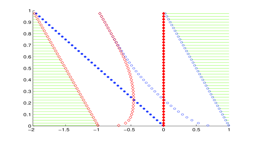
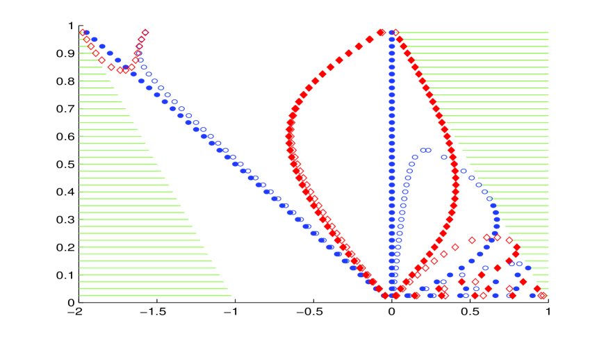
Figure 3: $\sigma(\eur{L}_{0})$. Eigenvalues (${\scriptscriptstyle\blacklozenge}$, $\bullet$; “even” and “odd”, respectively) and the values of $\lambda$ corresponding to antibound states (${\scriptscriptstyle\lozenge}$, $\circ$; also “even” and “odd”, respectively). We say that the eigenvalue is “even” (“odd”) if the first component of the corresponding eigenfunction is even (odd, respectively).

Figure 4: $\sigma(\eur{L}_{1})$. Eigenvalues (“even” ${\scriptscriptstyle\blacklozenge}$ and “odd” $\bullet$) and the values of $\lambda$ corresponding to antibound states (“even” ${\scriptscriptstyle\lozenge}$ and “odd” $\circ$).

6 Spectrum of $\eub{J}\eub{L}$

The analysis of the spectrum of $\eub{J}\eub{L}$ builds upon what has been discovered for the operators $\eur{L}_{0}$, $\eur{L}_{1}$ in Section 5. In particular, starting from the explicit eigenvectors for $\eur{L}_{0}$, $\eur{L}_{1}$ we are able to construct explicit eigenvectors for $\eub{J}\eub{L}$.

Lemma 6.1.

For any nonlinearity $g(s)$ in (2.2) with $g(0)=1$, for linearization at a solitary wave $\phi(x)e^{-i\omega t}$ with $|\omega|<1$, the following is true:

1. The spectrum of $\eub{J}\eub{L}$ is symmetric with respect to the real and imaginary axes.

2. The essential spectrum of $\eub{J}\eub{L}$ lies on the imaginary axis and is given by

   $$\sigma_{ess}(\eub{J}\eub{L})=i\mathbb{R}\setminus(-i(1-\omega),i(1-\omega)).$$

3. $\ker\eub{J}\eub{L}=\mathop{\rm Span}\left\langle\left[\begin{matrix}\partial_{x}\phi\\ 0\end{matrix}\right],\left[\begin{matrix}0\\ \phi\end{matrix}\right]\right\rangle,$ with $\phi=\left[\begin{matrix}v\\ u\end{matrix}\right]\in\mathbb{R}^{2}.$

4. The values $\lambda=\pm 2i\omega$ are eigenvalues of $\eub{J}\eub{L}$. The corresponding eigenvectors are $\left[\begin{matrix}\varphi\\ \pm i\varphi\end{matrix}\right]$, where $\varphi=\left[\begin{matrix}u\\ v\end{matrix}\right]$.

Remark 6.2.

More generally, it turns out that $\lambda=\pm 2\omega i$ are $L^{2}$-eigenvalues of $\eub{JL}$ which corresponds to a linearization at a solitary wave of nonlinear Dirac equation (2.1) with any nonlinearity $g(s)$ and in any dimension $n\geq 1$. These are embedded eigenvalues as long as $|\omega|>m/3$, where $m:=g(0)$. See [Com11].

Proof.

Let us show that $\sigma_{p}(\eub{JL})$ is symmetric with respect to $\mathop{\rm{R\hskip-1.0pte}}\nolimits\lambda=0$ and $\mathop{\rm{I\hskip-1.0ptm}}\nolimits\lambda=0$. Since $\eub{J}\eub{L}=\left[\begin{matrix}0&\eur{L}_{0}\\ -\eur{L}_{1}&0\end{matrix}\right]$, with both $\eur{L}_{\pm}$ real-valued, $\lambda\in\sigma(\eub{J}\eub{L})$ implies that if $\varPsi\in L^{2}(\mathbb{R},\mathbb{C}^{4})$ satisfies $\eub{J}\eub{L}\varPsi=\lambda\varPsi$ (in the sense of distributions), then $\overline{\varPsi(x)}$ satisfies $\eub{J}\eub{L}\bar{\varPsi}=\bar{\lambda}\bar{\varPsi}$. At the same time, the function $\bm{\varSigma}\varPsi(x)$, with $\bm{\varSigma}=\left[\begin{matrix}I_{2}&0\\ 0&-I_{2}\end{matrix}\right],$ satisfies

$$\eub{J}\eub{L}\bm{\varSigma}\varPsi=\eub{J}\bm{\varSigma}\eub{L}\varPsi=-\bm{\varSigma}\eub{J}\eub{L}\varPsi=-\lambda\bm{\varSigma}\varPsi.$$

It follows that both $\bar{\lambda}$ and $-\lambda$ are also eigenvalues of $\eub{JL}$, hence $\sigma_{p}(\eub{J}\eub{L})$ is symmetric with respect to the line $\mathop{\rm{I\hskip-1.0ptm}}\nolimits\lambda=0$ and with respect to the point $\lambda=0$.

To find the essential spectrum of $\eub{J}\eub{L}$, by the Weyl criterion, we need to consider the limit of $\eub{J}\eub{L}$ as $x\to\pm\infty$, substituting $v$, $u$ by zeros and $g$ by $g(0)=m=1$; then $\eub{J}\eub{L}-\lambda$ turns into $\eub{J}(\eub{D}-\omega)-\lambda$, where $\eub{D}=\left[\begin{matrix}\eur{D}&0\\ 0&\eur{D}\end{matrix}\right]$, with $\eur{D}=\left[\begin{matrix}1&\partial_{x}\\ -\partial_{x}&-1\end{matrix}\right]$ defined in (5.1). Substituting into $(\eub{J}(\eub{D}-\omega)-\lambda)\varPsi=0$ the Ansatz $\varPsi(x)=\varXi e^{i\xi x}$, with $\varXi\in\mathbb{C}^{4}$, $\varXi\neq 0$, we get:

$$(\eub{J}(\eub{D}-\omega)-\lambda)\varXi e^{i\xi x}=e^{i\xi x}(\eub{J}(\eub{D}(\xi)-\omega)-\lambda)\varXi=e^{i\xi x}\left[\begin{matrix}-\lambda&\eur{D}(\xi)-\omega\\ -\eur{D}(\xi)+\omega&-\lambda\end{matrix}\right]\varXi=0,$$

where $\eub{D}(\xi)=\left[\begin{matrix}\eur{D}(\xi)&0\\ 0&\eur{D}(\xi)\end{matrix}\right]$, with $\eur{D}(\xi)=\left[\begin{matrix}1&i\xi\\ -i\xi&-1\end{matrix}\right]$ being the symbol of $\eur{D}$. The essential spectrum of $\eub{J}\eub{L}$ is the range of values of $\lambda$ which correspond to $\xi\in\mathbb{R}$. To find the relation between $\lambda$ and $\xi$, we need to compute the determinant $\det\left(\eub{J}(\eub{D}(\xi)-\omega)-\lambda\right)$ and to equate it to zero. In order to compute the determinant, we notice that

$$\big{(}\eub{J}(\eub{D}(\xi)-\omega)-\lambda\big{)}\big{(}\eub{J}(\eub{D}(\xi)-\omega)+\lambda\big{)}=-(\eub{D}(\xi)-\omega)^{2}-\lambda^{2}=-\xi^{2}-1-\omega^{2}-\lambda^{2}+2\omega\eub{D}(\xi),$$

$$\big{(}-\xi^{2}-1-\omega^{2}-\lambda^{2}+2\omega\eub{D}(\xi)\big{)}\big{(}-\xi^{2}-1-\omega^{2}-\lambda^{2}-2\omega\eub{D}(\xi)\big{)}=\big{(}(1-\omega^{2}+\xi^{2}+\lambda^{2})^{2}+4\omega^{2}\lambda^{2}\big{)}{I}_{4},$$

where ${I}_{4}$ is the $4\times 4$ identity matrix. Since $\det\left(\eub{J}(\eub{D}(\xi)-\omega)-\lambda\right)$ should be even with respect to $\xi$ and $\omega$, two above relations allow us to conclude that $\det\left(\eub{J}(\eub{D}(\xi)-\omega)-\lambda\right)=(1-\omega^{2}+\xi^{2}+\lambda^{2})^{2}+4\omega^{2}\lambda^{2}.$ The equation

$$\det\left(\eub{J}(\eub{D}(\xi)-\omega)-\lambda\right)=(1-\omega^{2}+\xi^{2}+\lambda^{2})^{2}+4\omega^{2}\lambda^{2}=0$$

allows one to express $\lambda$ in terms of $\xi$ as $\lambda=\pm i(\omega\pm\sqrt{1+\xi^{2}}),$ or, vice versa,

$$\xi=\pm\sqrt{(\omega\pm i\lambda)^{2}-1}.$$

This shows that the essential spectrum is $i\mathbb{R}\backslash(-i(1-\omega),i(1-\omega))$.

The kernel of $\eub{J}\eub{L}$ is known by Lemma 5.4. Finally, again due to Lemma 5.4,

$$\eub{J}\eub{L}\left[\begin{matrix}\varphi\\ \pm i\varphi\end{matrix}\right]=\left[\begin{matrix}0&\eur{L}_{0}\\ -\eur{L}_{1}&0\end{matrix}\right]\left[\begin{matrix}\varphi\\ \pm i\varphi\end{matrix}\right]=-2\omega\left[\begin{matrix}\pm i\varphi\\ -\varphi\end{matrix}\right]=\mp 2\omega i\left[\begin{matrix}\varphi\\ \pm i\varphi\end{matrix}\right].$$

∎

Definition 6.3.

Threshold points are the values of $\lambda\in\mathbb{C}$ which correspond to $\xi=0$.

On Figure 5, one can see that the essential spectrum of $\eub{JL}$ consists of two overlapping components, which we distinguish by the symbols $\flat$ and $\sharp$. The $\flat$-component is $i\mathbb{R}\backslash(\lambda^{\flat}_{d},\lambda^{\flat}_{u})$, with the threshold points

$$\lambda^{\flat}_{d}=-i-i\omega,\qquad\lambda^{\flat}_{u}=i-i\omega;$$ (6.1)

the $\sharp$-component is $i\mathbb{R}\backslash(\lambda^{\sharp}_{d},\lambda^{\sharp}_{u})$, with the threshold points

$$\lambda^{\sharp}_{d}=-i+i\omega,\qquad\lambda^{\sharp}_{u}=i+i\omega.$$ (6.2)

We use the subscripts “$d$” and “$u$” for the lower (“down”) and the upper edges of each of the $\flat$, $\sharp$ components of the essential spectrum.

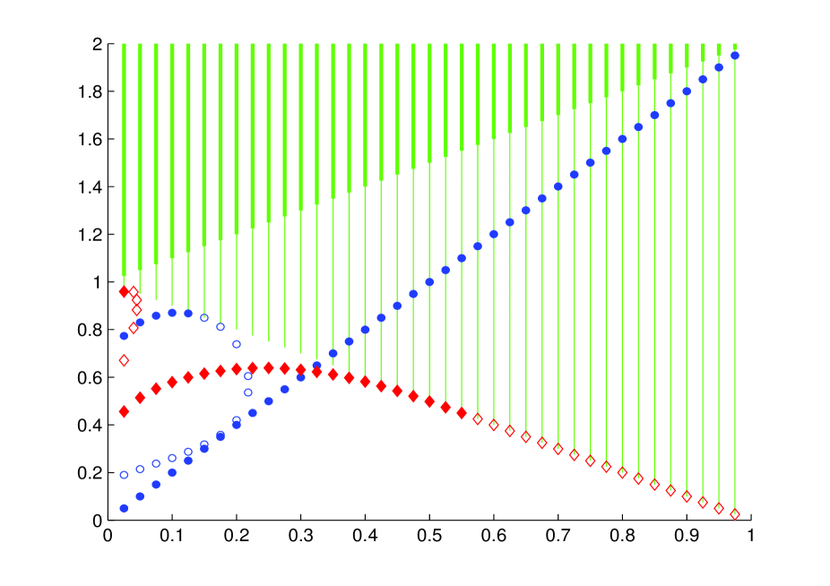
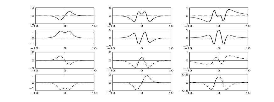
Figure 6: $\sigma(\eub{J}\eub{L})$. The zeros of the Evans function located in the upper half of the spectral gap (vertical axis) as a function of $\omega$ (horizontal axis). Eigenvalues (${\scriptscriptstyle\blacklozenge}$, $\bullet$) and the values of $\lambda$ corresponding to antibound states (${\scriptscriptstyle\lozenge}$, $\circ$). The eigenvalue $2\omega i$ (the straight line of $\bullet$) is embedded into the essential spectrum for $\omega>1/3$.

Figure 7: Components of the eigenfunctions corresponding to the eigenvalues $0.2000i$, $0.5792i$, and $0.8703i$ of $\eub{J}\eub{L}$, located in the upper half of the spectral gap for $\omega=0.1$. All three eigenfunctions have their first two components real-valued (solid lines) and second two components imaginary (dashed lines).

The numerical computation of the point spectrum of $\eub{J}\eub{L}$ inside $(0,i(1+\omega))$, as a function of $\omega\in(0,1)$, is plotted on Figure 7. The eigenfunctions corresponding to three point eigenvalues at $\omega=0.1$ are plotted on Figure 7.

7 Jost solutions and Evans functions

Looking for zeros of the Evans function is a way to test when an equation has solutions with the correct asymptotics at infinity. The definition involves two main steps. The first step is to construct Jost solutions, which are defined as solutions with certain decaying asymptotics either at plus infinity or at minus infinity. The second step is to match these two types of solutions. In the presence of symmetry the construction can be made simpler, simplifying the numerical computations. We describe this in detail below.

7.1 Jost solutions for $\eub{J}\eub{L}$

Jost solutions $Y(x,\lambda)$ of $\eub{J}\eub{L}$ are defined as solutions to $(\eub{J}\eub{L}-\lambda)\varPsi=0$ which have the same asymptotics at $+\infty$ or at $-\infty$ as the solutions to $(\eub{J}(\eub{D}-\omega)-\lambda)\varPsi=0$, where

$$\eub{D}=\left[\begin{matrix}\eur{D}&0\\ 0&\eur{D}\end{matrix}\right],\qquad\eur{D}=-i\alpha\partial_{x}+\beta=\left[\begin{matrix}1&\partial_{x}\\ -\partial_{x}&-1\end{matrix}\right].$$

For a given $\lambda\in\mathbb{C}$ away from the threshold points $\pm(1\pm\omega)i$, solutions to $(\eub{J}(\eub{D}-\omega)-\lambda)\varPsi=0$ have the form

$$\varPsi(x,\lambda)=\left[\begin{matrix}R\\ S\end{matrix}\right]e^{i\xi x},$$

where $\left[\begin{matrix}R\\ S\end{matrix}\right]\in\mathbb{C}^{4}$ and $\xi\in\mathbb{C}$ is a solution to $\det\left(\eub{J}(\eub{L}(\xi)-\omega)-\lambda\right)=0$. Let $\lambda=a+ib$, with $a\geq 0$ and $b\geq 0$. (Because of the symmetry of $\sigma(\eub{JL})$ with respect to the lines $\mathop{\rm{R\hskip-1.0pte}}\nolimits\lambda=0$ and $\mathop{\rm{I\hskip-1.0ptm}}\nolimits\lambda=0$, we only need to consider the spectrum in the closure of the first quadrant of $\mathbb{C}$.) Then define

$$\xi^{\flat}=\sqrt{((b-ia)+\omega)^{2}-1},\qquad\qquad\xi^{\sharp}=\sqrt{((b-ia)-\omega)^{2}-1},$$

where for the square root we choose the branch that has negative imaginary part (so that both $e^{-i\xi^{\flat}x}$ and $e^{-i\xi^{\sharp}x}$ decay as $x\to+\infty$). Then $\xi^{\flat}$ is defined for $\lambda\in\mathbb{C}$ with the cuts from $\lambda^{\flat}_{u}=i(1-\omega)$ to $+i\infty$ and from $\lambda^{\flat}_{d}=-i(1+\omega)$ to $-i\infty$, while $\xi^{\sharp}$ is defined for $\lambda\in\mathbb{C}$ with the cuts from $\lambda^{\sharp}_{u}=i(1+\omega)$ to $+i\infty$ and from $\lambda^{\sharp}_{d}=-i(1-\omega)$ to $-i\infty$. See Figure 5. Altogether the four solutions to the equation $\det\left(\eub{J}(\eub{D}(\xi)-\omega)-\lambda\right)=0$ are $\pm\xi^{\flat}(\lambda)$ and $\pm\xi^{\sharp}(\lambda)$.

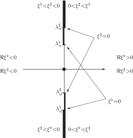
Figure 5: Domains of analytic functions $\xi^{\flat}(\lambda)$, $\xi^{\sharp}(\lambda)$, and the essential spectrum of $\eub{J}\eub{L}$. The thresholds are located at $\lambda^{\flat}_{d}=-i-i\omega$, $\lambda^{\sharp}_{d}=-i+i\omega$, $\lambda^{\flat}_{u}=i-i\omega$, and $\lambda^{\sharp}_{u}=i+i\omega$. The analytic function $\xi^{\flat}(\lambda)$ is defined on $\mathbb{C}$ with the cuts from $\lambda^{\flat}_{u}$ to $+i\infty$ and from $\lambda^{\flat}_{d}$ to $-i\infty$ (thick lines on the left side of the imaginary axis). $\mathop{\rm{I\hskip-1.0ptm}}\nolimits\xi^{\flat}<0$, $\mathop{\rm{I\hskip-1.0ptm}}\nolimits\xi^{\sharp}<0$ for all $\lambda\in\mathbb{C}$. The analytic function $\xi^{\sharp}(\lambda)$ is defined on $\mathbb{C}$ with the cuts from $\lambda^{\sharp}_{u}$ to $+i\infty$ and from $\lambda^{\sharp}_{d}$ to $-i\infty$ (thick lines on the right side of the imaginary axis). The boundary traces of both $\xi^{\sharp}$ and $\xi^{\flat}$ at the double-covered part of the essential spectrum (above $\lambda^{\sharp}_{u}$ and below $\lambda^{\flat}_{d}$) are real-valued.

The four solutions to $(\eub{J}(\eub{D}-\omega)-\lambda)\varPsi=0$ corresponding to $\lambda$ away from the thresholds (6.1), (6.2) are given by

$$\varXi^{\flat}_{\pm}(\lambda)e^{\pm\xi^{\flat}(\lambda)x},\qquad\varXi^{\sharp}_{\pm}(\lambda)e^{\pm\xi^{\sharp}(\lambda)x},$$ (7.1)

where

$$\varXi^{\flat}_{-}(\lambda)=\left[\begin{matrix}-i\xi^{\flat}(\lambda)\\ -i\lambda-1+\omega\\ \xi^{\flat}(\lambda)\\ \lambda-i(1-\omega)\end{matrix}\right],\qquad\varXi^{\sharp}_{-}(\lambda)=\left[\begin{matrix}-i\xi^{\sharp}(\lambda)\\ i\lambda-1+\omega\\ -\xi^{\sharp}(\lambda)\\ \lambda+i(1-\omega)\end{matrix}\right],$$ (7.2)

$$\qquad\varXi^{\flat}_{+}(\lambda)=\left[\begin{matrix}i\xi^{\flat}(\lambda)\\ -i\lambda-1+\omega\\ -\xi^{\flat}(\lambda)\\ \lambda-i(1-\omega)\end{matrix}\right],\qquad\varXi^{\sharp}_{+}(\lambda)=\left[\begin{matrix}i\xi^{\sharp}(\lambda)\\ i\lambda-1+\omega\\ \xi^{\sharp}(\lambda)\\ \lambda+i(1-\omega)\end{matrix}\right].$$ (7.3)

We will only be considering the Jost solutions which have prescribed asymptotics at $x\to+\infty$.

Lemma 7.1.

For each $\lambda\in\mathbb{C}$, $\lambda\notin\{\lambda^{\flat}_{d},\lambda^{\sharp}_{d},\lambda^{\flat}_{u},\lambda^{\sharp}_{u}\}$, there are Jost solutions to $(\eub{JL}-\lambda)\varPsi=0$ with the asymptotics $Y^{\sharp}_{\pm}(x,\lambda)\sim\varXi^{\sharp}_{\pm}(\lambda)e^{\pm i\xi^{\sharp}(\lambda)x}$ and $Y^{\flat}_{\pm}(x,\lambda)\sim\varXi^{\flat}_{\pm}(\lambda)e^{\pm i\xi^{\flat}(\lambda)x}$, $x\to+\infty$. More precisely,

$$|Y^{\sharp}_{\pm}(x,\lambda)e^{\mp i\xi^{\sharp}(\lambda)x}-\varXi^{\sharp}_{\pm}(\lambda)|=o(1),\qquad x\to+\infty;$$

$$|Y^{\flat}_{\pm}(x,\lambda)e^{\mp i\xi^{\flat}(\lambda)x}-\varXi^{\flat}_{\pm}(\lambda)|=o(1),\qquad x\to+\infty.$$

Proof.

The proof follows from the Duhamel representation for the solution to $(\eub{JL}-\lambda)\varPsi=0$ and from the exponential spatial decay of the solitary waves $\phi(x)$ corresponding to $\omega\in(0,1)$; see Remark 3.5. ∎

Remark 7.2.

At the threshold points $\lambda^{\sharp}_{d}=-i+i\omega$ and $\lambda^{\sharp}_{u}=i+i\omega$ (respectively, $\lambda^{\flat}_{d}=-i-i\omega$ and $\lambda^{\flat}_{u}=i-i\omega$), where $\xi^{\sharp}(\lambda)=0$ (respectively, $\xi^{\flat}(\lambda)=0$), one has $\varXi^{\sharp}_{+}(\lambda)=\varXi^{\sharp}_{-}(\lambda)$ (respectively, $\varXi^{\flat}_{+}(\lambda)=\varXi^{\flat}_{-}(\lambda)$). For such $\lambda$, there are only three Jost solutions as in Lemma 7.1, and one more Jost solution which is linearly growing as $x\to+\infty$.

7.2 Evans functions for $\eub{JL}$

Normally, Evans function describes a matching between Jost solutions decaying to the left and Jost solutions decaying to the right. However, presence of symmetries allows us to streamline calculation in the present case. Denote by $X^{{\scriptscriptstyle\blacklozenge}}$ the “even” subspace of functions from $C^{1}(\mathbb{R},\mathbb{C}^{4})$ with even first and third components and with odd second and fourth components. Similarly, denote by $X^{\bullet}$ the “odd” subspace in $C^{1}(\mathbb{R},\mathbb{C}^{4})$ with odd first and third components and with even second and fourth components. Then $C^{1}(\mathbb{R},\mathbb{C}^{4})=X^{{\scriptscriptstyle\blacklozenge}}\oplus X^{\bullet}$. Noticing that $\eub{J}\eub{L}$ acts invariantly in $X^{{\scriptscriptstyle\blacklozenge}}$ and in $X^{\bullet}$, we conclude that all eigenvalues of $\eub{J}\eub{L}$ always have a corresponding eigenfunction either in $X^{{\scriptscriptstyle\blacklozenge}}$ or in $X^{\bullet}$ (or in both subspaces). To find eigenvalues of $\eub{J}\eub{L}$ corresponding to functions from $X^{{\scriptscriptstyle\blacklozenge}}$, we proceed as follows:

• For $\lambda\in\mathbb{C}$, construct solutions $\varPsi_{j}$, $1\leq j\leq 4$, to the equation $\eub{J}\eub{L}\varPsi=\lambda\varPsi$ with the following initial data at $x=0$:

  $$\varPsi_{1}|_{{}_{x=0}}={\tiny\left[\begin{matrix}1\\ 0\\ 0\\ 0\end{matrix}\right]},\qquad\varPsi_{2}|_{{}_{x=0}}={\tiny\left[\begin{matrix}0\\ 1\\ 0\\ 0\end{matrix}\right]},\qquad\varPsi_{3}|_{{}_{x=0}}={\tiny\left[\begin{matrix}0\\ 0\\ 1\\ 0\end{matrix}\right]},\qquad\varPsi_{4}|_{{}_{x=0}}={\tiny\left[\begin{matrix}0\\ 0\\ 0\\ 1\end{matrix}\right]}.$$ (7.4)

  Then $\varPsi_{1}$, $\varPsi_{3}\in X^{{\scriptscriptstyle\blacklozenge}}$, while $\varPsi_{2}$, $\varPsi_{4}\in X^{\bullet}$.

• Take the Jost solutions $Y^{\flat}_{-}(x,\lambda)$ and $Y^{\sharp}_{-}(x,\lambda)$ as in Lemma 7.1, which decay for $x\to+\infty$.

• Define the Evans function

  $$E_{--}^{{\scriptscriptstyle\blacklozenge}}(\lambda)=\det\left[\varPsi_{1}(x,\lambda),\,\varPsi_{3}(x,\lambda),\,Y^{\flat}_{-}(x,\lambda),\,Y^{\sharp}_{-}(x,\lambda)\right].$$ (7.5)

  This is a Wronskian-type function which does not depend on $x$ and could be evaluated at $x=R\gg 1$, where the asymptotics of $Y^{\flat}_{-}$ and $Y^{\sharp}_{-}$ are known from Lemma 7.1. Vanishing of $E_{--}^{{\scriptscriptstyle\blacklozenge}}(\lambda)$ at particular $\lambda\in\mathbb{C}$ means that a certain linear combination of $\varPsi_{1}(x,\lambda)$ and $\varPsi_{3}(x,\lambda)$ has the asymptotics of the linear combination of $Y^{\flat}_{-}(x,\lambda)$ and $Y^{\sharp}_{-}(x,\lambda)$ as $x\to+\infty$, which decays at $+\infty$ (according to our choice of $\xi^{\flat}(\lambda)$ and $\xi^{\sharp}(\lambda)$. By the symmetry of $\varPsi$ (its first and third components are even while its second and fourth components are odd), this same linear combination also decays as $x\to-\infty$. Therefore, vanishing of $E_{--}^{{\scriptscriptstyle\blacklozenge}}(\lambda)$ at some $\lambda\in\mathbb{C}$ implies that there is an eigenfunction corresponding to this particular value of $\lambda$.

• Similarly, define

  $$E_{--}^{\bullet}(\lambda)=\det\left[\varPsi_{2}(x,\lambda),\,\varPsi_{4}(x,\lambda),\,Y^{\flat}_{-}(x,\lambda),\,Y^{\sharp}_{-}(x,\lambda)\right].$$ (7.6)

  The condition $E^{\bullet}(\lambda)=0$ means that a certain linear combination of $\varPsi_{2}$, $\varPsi_{4}\in X^{\bullet}$ has the same asymptotics when $x\to+\infty$ as a solution of $(\eub{J}(\eub{D}-\omega)-\lambda)\varPsi=0$ which decays for $x\to+\infty$.

Let us summarize the above in a convenient form:

Lemma 7.3.

$\lambda\in\sigma_{p}(\eub{J}\eub{L})$ if and only if $E_{--}^{{\scriptscriptstyle\blacklozenge}}(\lambda)E_{--}^{\bullet}(\lambda)=0$. Furthermore, $E_{--}^{{\scriptscriptstyle\blacklozenge}}(\lambda)=0$ (respectively, $E_{--}^{\bullet}(\lambda)=0$) if the corresponding wave function belongs to $L^{2}(\mathbb{R},\mathbb{C}^{4})\cap X^{{\scriptscriptstyle\blacklozenge}}$ (respectively, $L^{2}(\mathbb{R},\mathbb{C}^{4})\cap X^{\bullet}$).

When searching numerically for zeros of the Evans functions in the spectral gap on the imaginary axis, we benefit from the following observation.

Lemma 7.4.

For $\lambda\in i(-(1-\omega),(1-\omega))$, the real part of the functions $E_{--}^{{\scriptscriptstyle\blacklozenge}}(\lambda),$ $E_{--}^{\bullet}(\lambda)$ equals zero.

Proof.

For $\lambda$ with $\mathop{\rm{R\hskip-1.0pte}}\nolimits\lambda=0$, one immediately concludes from $(\eub{J}\eub{L}-\lambda)\varPsi_{j}=0$ that for all $x\in\mathbb{R}$ the components $(\varPsi_{1}(x))_{j}$ and $(\varPsi_{2}(x))_{j}$ are real for $j=1,\,2$ and imaginary for $j=3,\,4$, and that $(\varPsi_{3}(x))_{j}$ and $(\varPsi_{4}(x))_{j}$ are imaginary for $j=1,\,2$ and real for $j=3,\,4$. On the other hand, when $\lambda\in(-i(1-\omega),i(1-\omega))$ and both $\xi^{\flat}$ and $\xi^{\sharp}$ are imaginary, the first two components of $\varXi^{\flat}_{-}$ and $\varXi^{\sharp}_{-}$ from (7.2) are real and the second two are imaginary. It follows that

$$\det\left[\varPsi_{1}(x,\lambda),\varPsi_{3}(x,\lambda),\varXi^{\flat}_{-}(\lambda),\varXi^{\sharp}_{-}(\lambda)\right]\in i\mathbb{R},\qquad\det\left[\varPsi_{2}(x,\lambda),\varPsi_{4}(x,\lambda),\varXi^{\flat}_{-}(\lambda),\varXi^{\sharp}_{-}(\lambda)\right]\in i\mathbb{R},$$

for any $x\in\mathbb{R}$. Since $\xi^{\flat}$ and $\xi^{\sharp}$ are purely imaginary, $e^{-i\xi^{\flat}x}$ and $e^{-i\xi^{\sharp}x}$ are real; we conclude from Lemma 7.1 that

$$E_{--}^{{\scriptscriptstyle\blacklozenge}}(\lambda)=\det\left[\varPsi_{1}(x,\lambda),\varPsi_{3}(x,\lambda),Y^{\flat}_{-}(\lambda),Y^{\sharp}_{-}(\lambda)\right]$$

and

$$E_{--}^{\bullet}(\lambda)=\det\left[\varPsi_{2}(x,\lambda),\varPsi_{4}(x,\lambda),Y^{\flat}_{-}(\lambda),Y^{\sharp}_{-}(\lambda)\right]$$

are purely imaginary. ∎

7.3 Jost solutions and Evans functions for $\eur{L}_{0}$ and $\eur{L}_{1}$

The construction of the Jost solutions and Evans function for the operator $\eur{L}_{1}$ (and, respectively, $\eur{L}_{0}$) is similar to the construction for $\eub{J}\eub{L}$. At $x\to\pm\infty$, $\eur{L}_{1}$ coincides with $\eur{D}-\omega$. The equation

$$(\eur{D}-\omega-\lambda)\Psi(x)=0$$

has two linearly independent solutions

$$\Xi_{\pm}(\lambda)e^{\pm i\xi(\lambda)x},$$

where $\Xi_{\pm}(\lambda)\in\mathbb{C}^{2}$ are given by

$$\Xi_{\pm}(\lambda)=\left[\begin{array}[]{c}1+\omega+\lambda\\ \mp i\xi(\lambda)\end{array}\right],\qquad\mbox{where}\quad\xi=\sqrt{(\omega+\lambda)^{2}-1}.$$

The function $\xi(\lambda)$ is defined for $\lambda\in\mathbb{C}$ with branch cuts from $\lambda=1-\omega$ to $+\infty$ and from $\lambda=-1-\omega$ to $-\infty$. These branch cuts correspond to the essential spectrum of the operator $\eur{L}_{1}$ (similarly, of $\eur{L}_{0}$). The square root denotes the branch with the negative imaginary part when the argument is negative, so that for $\lambda$ from the spectral gap $(-1-\omega,1-\omega)$, the function $\Xi_{-}(\lambda)e^{-i\xi(\lambda)x}$ is decaying as $x\to+\infty$. The Jost solutions ${\rm Y}_{\pm}(x,\lambda)$ for $\eur{L}_{1}$ are solutions to $(\eur{L}_{1}-\lambda){\rm Y}(x,\lambda)=0$ with the asymptotic behavior

$${\rm Y}_{\pm}(x,\lambda)\sim\Xi_{\pm}(\lambda)e^{\pm i\xi(\lambda)x},\qquad x\to+\infty.$$ (7.7)

There are two subspaces of $C^{1}(\mathbb{R},\mathbb{C}^{2})$, ${\rm X}^{{\scriptscriptstyle\blacklozenge}}$ (spinors with the even first component and odd second component) and ${\rm X}^{\bullet}$ (spinors with the odd first component and even second component) such that ${\rm X}^{{\scriptscriptstyle\blacklozenge}}\oplus{\rm X}^{\bullet}=C^{1}(\mathbb{R},\mathbb{C}^{2})$, which are invariant with respect to $\eur{L}_{1}$ (also with respect to $\eur{L}_{0}$). We define two solutions, $\Psi_{1}(x,\lambda)$ and $\Psi_{2}(x,\lambda)$, to the equation $(\eur{L}_{1}-\lambda)\Psi=0$, with the initial data

$$\Psi_{1}|_{{}_{x=0}}=\left[\begin{matrix}1\\ 0\end{matrix}\right],\qquad\Psi_{2}|_{{}_{x=0}}=\left[\begin{matrix}0\\ 1\end{matrix}\right].$$

Then we define the Evans functions of $\eur{L}_{1}$ by

$${\rm E}_{\pm}^{{\scriptscriptstyle\blacklozenge}}(\lambda)=\det\left[\Psi_{1}(x,\lambda),\,{\rm Y}_{\pm}(x,\lambda)\right],\qquad{\rm E}_{\pm}^{\bullet}(\lambda)=\det\left[\Psi_{2}(x,\lambda),\,{\rm Y}_{\pm}(x,\lambda)\right],$$ (7.8)

and look for their zeros.

If ${\rm E}_{-}^{\scriptscriptstyle\blacklozenge}(\lambda)$ vanishes at some $\lambda\in\mathbb{C}$, then it means that $\Psi_{1}(x,\lambda)$ as $x\to+\infty$ has the asymptotics of the decaying Jost solution. (By the symmetry, as $x\to-\infty$, $\Psi_{1}(x,\lambda)$ also has the asymptotics of the Jost solution decaying to $-\infty$.) We can summarize this as follows.

Lemma 7.5.

The inclusion $\lambda\in\sigma_{p}(\eur{L}_{1})$ takes place if and only if ${\rm E}_{-}^{{\scriptscriptstyle\blacklozenge}}(\lambda){\rm E}_{-}^{\bullet}(\lambda)=0$.

In the same way one defines the Evans functions ${\rm E}^{{\scriptscriptstyle\blacklozenge}}_{-}(\lambda)$ and ${\rm E}^{\bullet}_{-}(\lambda)$ for $\eur{L}_{0}$. The zeros of the Evans functions ${\rm E}^{{\scriptscriptstyle\blacklozenge}}_{\pm}(\lambda)$ and ${\rm E}^{\bullet}_{\pm}(\lambda)$ are plotted on Figure 4 (for $\eur{L}_{0}$) and Figure 4 (for $\eur{L}_{1}$). The meaning of zeros of ${\rm E}_{+}^{\scriptscriptstyle\blacklozenge}$ and ${\rm E}_{+}^{\bullet}$ is discussed in Section 7.4.

7.4 Antibound states for $\eur{L}_{0}$ and $\eur{L}_{1}$

The Evans function is defined using two pieces of data: a solution with the given initial data and the Jost solution that corresponds to one value of $\xi$, see equation (7.7). However, we can view $\xi(\lambda)$ as defined on a Riemann surface with two sheets (corresponding to $+\sqrt{\cdot}$ and $-\sqrt{\cdot}$) and two singularity points at $\pm 1-\omega$. The two sheets are glued across the cuts $(-\infty,-1-\omega]$ and $[1-\omega,\infty)$. The two eigenvectors of $\eur{D}-\omega$ (this operator coincides with $\eur{L}_{0}$ and $\eur{L}_{1}$ at $x\to\pm\infty$) can be thought of as the same eigenvector that changes according to which sheet $\lambda$ is on. Continuing in this vein, we consider two previously defined Jost solutions ${\rm Y}_{\pm}(x,\lambda)$, $\lambda\in\mathbb{C}\backslash\big{(}(-\infty,-1-\omega)\cup(1-\omega,+\infty)\big{)}$, as one Jost solution defined on the Riemann surface, which is glued of two copies of $\mathbb{C}\backslash\big{(}(-\infty,-1-\omega)\cup(1-\omega,+\infty)\big{)}$. We use this Jost solution to define the Evans function on this Riemann surface. Thus, for $\lambda$ on the first sheet of the Riemann surface, the Evans functions ${\rm E}^{{\scriptscriptstyle\blacklozenge}}(\lambda)$, ${\rm E}^{\bullet}(\lambda)$ are represented by ${\rm E}^{{\scriptscriptstyle\blacklozenge}}_{-}(\lambda)$, ${\rm E}^{\bullet}_{-}(\lambda)$ from (7.8), while on the second sheet they are represented by ${\rm E}^{{\scriptscriptstyle\blacklozenge}}_{+}(\lambda)$, ${\rm E}^{\bullet}_{+}(\lambda)$. When a zero of the Evans function disappears at the end of the spectral gap, it does not “dissolve” in the essential spectrum, but, rather, it goes back into the gap, albeit on a different sheet of the Riemann surface on which the Evans function is defined. Such an “unphysical” zero of the Evans function is known in the literature as a “resonance” or an “antibound state”. Since the “resonance” is also a name used specifically for a bounded solution at the threshold of the essential spectrum (at the threshold, the two notions coincide), we will be using the “antibound state” as the name of choice. It is “antibound” since the solution is purely exponentially increasing as $x\to\pm\infty$, consisting solely of ${\rm Y}_{+}(x,\lambda)$ as $x\to+\infty$.

On Figure 4 the antibound states of $\eur{L}_{1}$ are indicated by transparent symbols (${\scriptscriptstyle\lozenge}$ is for the states with even eigenfunctions and $\circ$ is for the states with odd eigenfunctions). Sometimes antibound states pass from the unphysical sheet onto the physical one at the threshold point $\lambda=1-\omega$. Note that the curve of transparent circles on the right has a maximum. This is the value of $\omega$ (on the vertical axis) at which two zeros of the Evans function living off the real axis $\mathop{\rm{I\hskip-1.0ptm}}\nolimits\lambda=0$ on the unphysical sheet collide and create two zeros on the real axis. The self-adjointness of the operator $\eur{L}_{1}$ forbids such a behaviour on the physical sheet, but it is possible on the unphysical one.

Antibound states for the operator $\eur{L}_{0}$ are plotted on Figure 4.

7.5 Antibound states for $\eub{JL}$

The Riemann surface on which the Evans function of the operator $\eub{JL}$ is defined is similar but more complicated. Indeed, the two limiting frequencies $\xi^{\flat}$ and $\xi^{\sharp}$ are defined on a two-sheeted surface each, but the surfaces are different. The Evans function is then defined on four sheets. We will denote them by $(+,+)$, $(+,-)$, $(-,+)$, $(-,-)$, depending on the sign in front of $(\xi^{\flat},\xi^{\sharp})$. The sheet $(-,-)$ is the physical one, in the sense that the zeros of the Evans function on this sheet are the eigenvalues of the operator $\eub{JL}$.

The sheets are glued in the following manner.

Across the cuts $(\lambda^{\sharp}_{u},i\infty)$ and $(\lambda^{\flat}_{d},-i\infty)$, the sheet $(+,+)$ is glued to $(-,-)$, while the sheet $(+,-)$ is glued to $(-,+)$ (that is, both signs change to their opposites).

Across the cut $(\lambda^{\flat}_{u},\lambda^{\sharp}_{u})$, the gluing is $(+,\cdot)\leftrightarrow(-,\cdot)$ (only the sign of $\xi^{\flat}$ changes), while across the cut $(\lambda^{\flat}_{d},\lambda^{\sharp}_{d})$ the sign of $\xi^{\sharp}$ changes: $(\cdot,+)\leftrightarrow(\cdot,-)$.

The four branches of the Evans function $E^{{\scriptscriptstyle\blacklozenge}}$ on these sheets could be written as follows:

$$E^{{\scriptscriptstyle\blacklozenge}}_{--}(\lambda)=\det\left[\varPsi_{1}(x,\lambda),\varPsi_{3}(x,\lambda),Y^{\flat}_{-}(x,\lambda),Y^{\sharp}_{-}(x)\right],$$

$$E^{{\scriptscriptstyle\blacklozenge}}_{+-}(\lambda)=\det\left[\varPsi_{1}(x,\lambda),\varPsi_{3}(x,\lambda),Y^{\flat}_{+}(x),Y^{\sharp}_{-}(x)\right],$$

$$E^{{\scriptscriptstyle\blacklozenge}}_{-+}(\lambda)=\det\left[\varPsi_{1}(x,\lambda),\varPsi_{3}(x,\lambda),Y^{\flat}_{-}(x,\lambda),Y^{\sharp}_{+}(x)\right],$$

$$E^{{\scriptscriptstyle\blacklozenge}}_{++}(\lambda)=\det\left[\varPsi_{1}(x,\lambda),\varPsi_{3}(x,\lambda),Y^{\flat}_{+}(x),Y^{\sharp}_{+}(x)\right].$$

Similarly one defines the four branches of the Evans function $E^{\bullet}$.

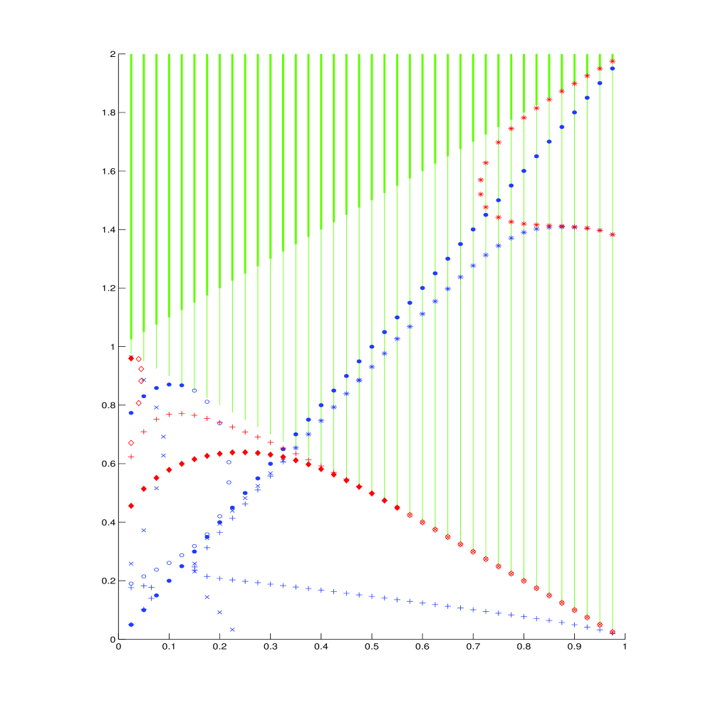
Figure 8: $\sigma(\eub{J}\eub{L})$. The zeros of the Evans function on the upper half of the imaginary axis (vertical) as a function of $\omega$ (horizontal axis). Eigenvalues (${\scriptscriptstyle\blacklozenge}$ for even eigenfunctions, $\bullet$ for odd) and the values of $\lambda$ corresponding to antibound states (${\scriptscriptstyle\lozenge}$ for even, $\circ$ for odd). The symbols ”$+$” and “$\times$” denote zeros of the Evans functions which correspond to to the Jost solutions on the other unphysical sheets (sheets $(-,+)$ and $(+,+)$) of the Riemann surface; see Section 7.4. The star symbols found inside the essential spectrum are actually made up of coinciding symbols “$+$” and “$\times$”; see Lemma 7.6.

In Figure 8 we trace the zeros of the Evans function on the $(-,-)$ sheet (eigenvalues, solid symbols) as well as the zeros on the $(+,-)$ sheet (“antibound states”, transparent symbols). The zeros can change between the two sheets by hitting the (square root type) singularity at $\lambda^{\flat}_{u}$. Note that when a curve has infinite derivative (with respect to $\omega$ on the $x$-axis) it signals that the zeros of Evans function are leaving the imaginary axis into the complex plane away from $\mathop{\rm{R\hskip-1.0pte}}\nolimits\lambda=0$. This behaviour can be seen for zeros on the $(+,-)$ sheet, but we have not observed it for the eigenvalues, which are the zeros on the $(-,-)$ sheet. This suggests that the eigenvalues stay on the imaginary axis for all values of $\omega$.

The zeros lying on the other two sheets are unlikely to sneak onto the “physical” $(-,-)$ sheet to become eigenvalues for the following reason. To pass onto this sheet, they would either have to leave the imaginary axis and circle around or to go inside the essential spectrum and hit the singularity at the embedded threshold at $\lambda^{\sharp}_{u}$. We have not observed such a hypothetical behaviour.

For completeness, we also plot on Figure 8 the zeros of Evans functions on the $(-,+)$ sheet and on the $(+,+)$ sheet. Note that between the thresholds $\lambda^{\flat}_{u}$ and $\lambda^{\sharp}_{u}$, these zeros (marked on Figure 8 with “$+$” and “$\times$”) meet. Indeed, there is the following simple observation.

Lemma 7.6.

For $\lambda\in(\lambda^{\flat}_{d},\lambda^{\sharp}_{d})\cup(\lambda^{\flat}_{u},\lambda^{\sharp}_{u})$,

$$E_{-+}^{{\scriptscriptstyle\blacklozenge}}(\lambda)=\overline{E_{++}^{{\scriptscriptstyle\blacklozenge}}(\lambda)},\qquad E_{-+}^{\bullet}(\lambda)=\overline{E_{++}^{\bullet}(\lambda)}.$$

Proof.

First, we notice that for $\lambda\in i\mathbb{R}$, if $\varPsi$ is a solution to

$$\eub{JL}\varPsi=\left[\begin{matrix}0&\eur{L}_{0}\\ -\eur{L}_{1}&0\end{matrix}\right]\varPsi=\lambda\varPsi,$$ (7.9)

then so is $\bm{\varSigma}\overline{\varPsi}$, where $\bm{\varSigma}=\left[\begin{matrix}{I}_{2}&0\\ 0&-{I}_{2}\end{matrix}\right]$. From (7.4), we conclude that for $\lambda\in i\mathbb{R}$,

$$\overline{\varPsi_{1}(x,\lambda)}=\bm{\varSigma}\varPsi_{1}(x,\lambda),\qquad\overline{\varPsi_{2}(x,\lambda)}=\bm{\varSigma}\varPsi_{2}(x,\lambda),\noindent$$ (7.10)

$$\overline{\varPsi_{3}(x,\lambda)}=-\bm{\varSigma}\varPsi_{3}(x,\lambda),\qquad\overline{\varPsi_{4}(x,\lambda)}=-\bm{\varSigma}\varPsi_{4}(x,\lambda).$$ (7.11)

For $\lambda\in(\lambda^{\flat}_{u},\lambda^{\sharp}_{u})$, since $\xi^{\flat}(\lambda)$ is real and $\xi^{\sharp}(\lambda)$ is imaginary, and taking into account (7.2) and (7.3), we see that there are the relations

$$\overline{\varXi^{\flat}_{+}(\lambda)e^{i\xi^{\flat}(\lambda)x}}=\bm{\varSigma}\varXi^{\flat}_{-}(\lambda)e^{-i\xi^{\flat}(\lambda)x},\qquad\overline{\varXi^{\sharp}_{+}(\lambda)e^{i\xi^{\sharp}(\lambda)x}}=\bm{\varSigma}\varXi^{\sharp}_{+}(\lambda)e^{i\xi^{\sharp}(\lambda)x}.$$ (7.12)

Given the Jost solutions $Y^{\flat}_{\pm}(x,\lambda)$ and $Y^{\sharp}_{\pm}(x,\lambda)$ which satisfy $(\eub{JL}-\lambda)\varPsi=0$, with $\lambda\in i\mathbb{R}$, we know that $\bm{\varSigma}\overline{Y^{\flat}_{\pm}(x,\lambda)}$ and $\bm{\varSigma}\overline{Y^{\sharp}_{\pm}(x,\lambda)}$ also satisfy $(\eub{JL}-\lambda)\varPsi=0$. Matching the asymptotics of the Jost solutions with (7.12) (see Lemma 7.1), we conclude that

$$\overline{Y^{\flat}_{+}(x,\lambda)}=\bm{\varSigma}Y^{\flat}_{-}(x,\lambda),\qquad\overline{Y^{\sharp}_{+}(x,\lambda)}=\bm{\varSigma}Y^{\sharp}_{+}(x,\lambda).$$ (7.13)

Taking into account (7.10) and (7.13), we have:

$$\overline{E^{{\scriptscriptstyle\blacklozenge}}_{-+}}=\det\left[\overline{\varPsi_{1}},\overline{\varPsi_{3}},\overline{Y^{\flat}_{-}},\overline{Y^{\sharp}_{+}}\right]=\det\left[\bm{\varSigma}\varPsi_{1},-\bm{\varSigma}\varPsi_{3},\bm{\varSigma}Y^{\flat}_{+},\bm{\varSigma}Y^{\sharp}_{+}\right]=\det\left[\varPsi_{1},-\varPsi_{3},Y^{\flat}_{+},Y^{\sharp}_{+}\right]=E^{{\scriptscriptstyle\blacklozenge}}_{++}.$$

In the same manner one proves that $\overline{E^{\bullet}_{-+}(\lambda)}=E^{\bullet}_{++}(\lambda)$ for $\lambda\in(\lambda^{\flat}_{u},\lambda^{\sharp}_{u})$.

The proof for $\lambda\in(\lambda^{\flat}_{d},\lambda^{\sharp}_{d})$ is similar. ∎

8 Conclusion

We considered the spectrum of the nonlinear Dirac equation in 1D, linearized at a solitary wave solution. The numeric simulations have been performed for the nonlinearity $g(s)=1-s$ (the Soler model), while some of our analytical conclusions remain valid for any nonlinearity.

In particular, we found that for any nonlinearity $g(s)$ there are the eigenvalues $\pm 2\omega i$ of the linearization $\eub{J}\eub{L}$. For a certain range of $\omega$, these eigenvalues are embedded in the essential spectrum of $\eub{J}\eub{L}$.

For the nonlinear Dirac equation with the nonlinearity $g(s)=1-s$ we have not found any other embedded eigenvalues of $\eub{J}\eub{L}$. We have not found any complex eigenvalues off the imaginary axis, concluding that the linearization at all solitary waves is spectrally stable.

References

- [BC11] N. Boussaid and S. Cuccagna, On stability of standing waves of nonlinear Dirac equations, ArXiv e-prints, 1103.4452 (2011).
- [BP93] V. S. Buslaev and G. S. Perel′man, Scattering for the nonlinear Schrödinger equation: states that are close to a soliton, St. Petersburg Math. J., 4 (1993), pp. 1111–1142.
- [BS03] V. S. Buslaev and C. Sulem, On asymptotic stability of solitary waves for nonlinear Schrödinger equations, Ann. Inst. H. Poincaré Anal. Non Linéaire, 20 (2003), pp. 419–475.
- [Chu07] M. Chugunova, Spectral stability of nonlinear waves in dynamical systems (Doctoral Thesis), McMaster University, Hamilton, Ontario, Canada, 2007.
- [CM08] S. Cuccagna and T. Mizumachi, On asymptotic stability in energy space of ground states for nonlinear Schrödinger equations, Comm. Math. Phys., 284 (2008), pp. 51–77.
- [Com11] A. Comech, On the meaning of the Vakhitov-Kolokolov stability criterion for the nonlinear Dirac equation, ArXiv e-prints, 1107.1763 (2011).
- [Cuc01] S. Cuccagna, Stabilization of solutions to nonlinear Schrödinger equations, Comm. Pure Appl. Math., 54 (2001), pp. 1110–1145.
- [CV86] T. Cazenave and L. Vázquez, Existence of localized solutions for a classical nonlinear Dirac field, Comm. Math. Phys., 105 (1986), pp. 35–47.
- [Der64] G. H. Derrick, Comments on nonlinear wave equations as models for elementary particles, J. Mathematical Phys., 5 (1964), pp. 1252–1254.
- [GN74] D. J. Gross and A. Neveu, Dynamical symmetry breaking in asymptotically free field theories, Phys. Rev. D, 10 (1974), pp. 3235–3253.
- [GO10] V. Georgiev and M. Ohta, Nonlinear instability of linearly unstable standing waves for nonlinear Schrödinger equations, ArXiv e-prints, 1009.5184 (2010).
- [Gri88] M. Grillakis, Linearized instability for nonlinear Schrödinger and Klein-Gordon equations, Comm. Pure Appl. Math., 41 (1988), pp. 747–774.
- [Gro66] L. Gross, The Cauchy problem for the coupled Maxwell and Dirac equations, Comm. Pure Appl. Math., 19 (1966), pp. 1–15.
- [GSS87] M. Grillakis, J. Shatah, and W. Strauss, Stability theory of solitary waves in the presence of symmetry. I, J. Funct. Anal., 74 (1987), pp. 160–197.
- [LG75] S. Y. Lee and A. Gavrielides, Quantization of the localized solutions in two-dimensional field theories of massive fermions, Phys. Rev. D, 12 (1975), pp. 3880–3886.
- [PS10] D. E. Pelinovsky and A. Stefanov, Asymptotic stability of small gap solitons in the nonlinear Dirac equations, ArXiv e-prints, 1008.4514 (2010).
- [Sha83] J. Shatah, Stable standing waves of nonlinear Klein-Gordon equations, Comm. Math. Phys., 91 (1983), pp. 313–327.
- [Sha85] J. Shatah, Unstable ground state of nonlinear Klein-Gordon equations, Trans. Amer. Math. Soc., 290 (1985), pp. 701–710.
- [Sol70] M. Soler, Classical, stable, nonlinear spinor field with positive rest energy, Phys. Rev. D, 1 (1970), pp. 2766–2769.
- [SS85] J. Shatah and W. Strauss, Instability of nonlinear bound states, Comm. Math. Phys., 100 (1985), pp. 173–190.
- [SW92] A. Soffer and M. I. Weinstein, Multichannel nonlinear scattering for nonintegrable equations. II. The case of anisotropic potentials and data, J. Differential Equations, 98 (1992), pp. 376–390.
- [SW99] A. Soffer and M. I. Weinstein, Resonances, radiation damping and instability in Hamiltonian nonlinear wave equations, Invent. Math., 136 (1999), pp. 9–74.
- [VK73] N. G. Vakhitov and A. A. Kolokolov, Stationary solutions of the wave equation in the medium with nonlinearity saturation, Radiophys. Quantum Electron., 16 (1973), pp. 783–789.
- [Wei85] M. I. Weinstein, Modulational stability of ground states of nonlinear Schrödinger equations, SIAM J. Math. Anal., 16 (1985), pp. 472–491.
- [Wei86] M. I. Weinstein, Lyapunov stability of ground states of nonlinear dispersive evolution equations, Comm. Pure Appl. Math., 39 (1986), pp. 51–67.
- [Zak67] V. Zakharov, Instability of self-focusing of light, Zh. Éksp. Teor. Fiz, 53 (1967), pp. 1735–1743.