Bidding for Representative Allocations for Display Advertising

Abstract

Display advertising has traditionally been sold via guaranteed contracts – a guaranteed contract is a deal between a publisher and an advertiser to allocate a certain number of impressions over a certain period, for a pre-specified price per impression. However, as spot markets for display ads, such as the RightMedia Exchange, have grown in prominence, the selection of advertisements to show on a given page is increasingly being chosen based on price, using an auction. As the number of participants in the exchange grows, the price of an impressions becomes a signal of its value. This correlation between price and value means that a seller implementing the contract through bidding should offer the contract buyer a range of prices, and not just the cheapest impressions necessary to fulfill its demand.

Implementing a contract using a range of prices, is akin to creating a mutual fund of advertising impressions, and requires randomized bidding. We characterize what allocations can be implemented with randomized bidding, namely those where the desired share obtained at each price is a non-increasing function of price. In addition, we provide a full characterization of when a set of campaigns are compatible and how to implement them with randomized bidding strategies.

1 Introduction

Display advertising — showing graphical ads on regular web pages, as opposed to textual ads on search pages — is approximately a $24 billion business. There are two ways in which an advertiser looking to reach a specific audience (for example, 10 million males in California in July 2009) can buy such ad placements. One is the traditional method, where the advertiser enters into an agreement, called a guaranteed contract, directly with the publishers (owners of the webpages). Here, the publisher guarantees to deliver a prespecified number (10 million) of impressions matching the targeting requirements (male, from California) of the contract in the specified time frame (July 2009). The second is to participate in a spot market for display ads, such as the RightMedia Exchange, where advertisers can buy impressions one pageview at a time: every time a user loads a page with a spot for advertising, an auction is held where advertisers can bid for the opportunity to display a graphical ad to this user. Both the guaranteed and spot markets for display advertising now thrive side-by-side. There is demand for guaranteed contracts from advertisers who want to hedge against future uncertainty of supply. For example, an advertiser who must reach a certain audience during a critical period of time (e.g around a forthcoming product launch, such as a movie release) may not want to risk the uncertainty of a spot market; a guaranteed contract insures the publisher as well against fluctuations in demand. At the same time, a spot market allows the advertisers to bid for specific opportunities, permitting very fine grained targeting based on user tracking. Currently, RightMedia runs over nine billion auctions for display ads everyday.

How should a publisher decide which of her supply of impressions to allocate to her guaranteed contracts, and which to sell on the spot market? One obvious solution is to fulfill the guaranteed demand first, and then sell the remaining inventory on the spot market. However, spot market prices are often quite different for two impressions that both satisfy the targeting requirements of a guaranteed contract, since different impressions have different value. For example, the impressions from two users with identical demographics can have different value, based on different search behavior reflecting purchase intent for one of the users, but not the other. Since advertisers on the spot market have access to more tracking information about each user, the resulting bids may be quite different for these two users. Allocating impressions to guaranteed contracts first and selling the remainder on the spot market can therefore be highly suboptimal in terms of revenue, since two impressions that would fetch the same revenue from the guaranteed contract might fetch very different prices from the spot market.

On the other hand, simply buying the cheapest impressions on the spot market to satisfy guaranteed demand is not a good solution in terms of fairness to the guaranteed contracts, and leads to increasing short term revenue at the cost of long term satisfaction. As discussed above, impressions in online advertising have a common value component because advertisers generally have different information about a given user. This information (e.g. browsing history on an advertiser site) is typically relevant to all of the bidders, even though only one bidder may possess this information. In such settings, price is a signal of value— in a model of valuations incorporating both common and private values, the price converges to the true value of the item in the limit as the number of bidders goes to infinity ([7, 10], see also [6] for discussion). On average, therefore, the price on the spot market is a good indicator of the value of the impression, and delivering cheapest impressions corresponds to delivering the lowest quality impressions to the guaranteed contract.

A publisher with access to both sources of demand thus faces a trade-off between revenue and fairness when deciding which impressions to allocate to the guaranteed contract; this trade-off is further compounded by the fact that the publisher typically does not have access to all the information that determines the value of a particular impression. Indeed, publishers are often the least well informed participants about the value of running an ad in front of a user. For example, when a user visits a politics site, Amazon (as an advertiser) can see that the user recently searched Amazon for an ipod, and Target (as an advertiser) can see they searched target.com for coffee mugs, but the publisher only knows the user visited the politics site. Furthermore, the exact nature of this trade-off is unknown to the publisher in advance, since it depends on the spot market bids which are revealed only after the advertising opportunity is placed on the spot market.

The publisher as a bidder. To address the problem of unknown spot market demand (i.e., the publisher would like to allocate the opportunity to a bidder on the spot market if the bid is “high enough”, else to a guaranteed contract), the publisher acts, in effect, as a bidder on behalf on the guaranteed contracts. That is, the publisher now plays two roles: that of a seller, by placing his opportunity on the spot market, and that of a bidding agent, bidding on behalf of his guaranteed contracts. If the publisher’s own bid turns out to be highest among all bids, the opportunity is won and is allocated to the guaranteed contract. Acting as a bidder allows the publisher to probe the spot market and decide whether it is more efficient to allocate the opportunity to an external bidder or to a guaranteed contract.

How should a publisher model the trade-off between fairness and revenue, and having decided on a trade-off, how should she place bids on the spot market? An ideal solution is (a) easy to implement, (b) allows for a trade-off between the quality of impressions delivered to the guaranteed contracts and short-term revenues, and (c) is robust to the exact tradeoff chosen. In this work we show precisely when such an ideal solution exists and how it can be implemented.

1.1 Our Contributions

In this paper, we provide an analytical framework to model the publisher’s problem of how to fulfill guaranteed advance contracts in a setting where there is an alternative spot market, and advertising opportunities have a common value component. We give a solution where the publisher bids on behalf of its guaranteed contracts in the spot market. The solution consists of two components: an allocation, specifying the fraction of impressions at each price allocated to a contract, and a bidding strategy, which specifies how to acquire this allocation by bidding in an auction.

The quality, or value, of an opportunity is measured by its price . A perfectly representative allocation is one which consists of the same proportion of impressions at every price– i.e., a mix of high-quality and low quality impressions. The trade-off between revenue and fairness is modeled using a budget, or average target spend constraint, for each advertiser’s allocation: the publisher’s choice of target spend reflects her trade-off between short-term revenue and quality of impressions for that advertiser (this must, of course, be large enough to ensure that the promised number of impressions satisfying the targeting constraints can be delivered.) Given a target spend , a maximally representative allocation is one which minimizes the distance to the perfectly representative allocation, subject to the budget constraint. We first show how to solve for a maximally representative allocation, and then show how to implement such an allocation by purchasing opportunities in an auction, using randomized bidding strategies.

Organization. We start out with the single contract case, where the publisher has just one existing guaranteed contract, in Section 2; this case is enough to illustrate the idea of maximally representative allocations and implementation via randomized bidding strategies. We move on to the more realistic case of multiple contracts in Section 3; we first prove a result about which allocations can be implemented in an auction in a decentralized fashion, and derive the corresponding decentralized bidding strategies. Next we solve for the optimal allocation when there are multiple contracts. Finally, in Section 4, we validate these strategies by simulating on data derived from real world exchanges.

1.1.1 Related Work

The most relevant work is the literature on designing expressive auctions and clearing algorithms for online advertising [8, 2, 9]. This literature does not address our problem for the following reason. While it is true that guaranteed contracts have coarse targeting relative to what is possible on the spot market, most advertisers with guaranteed contracts choose not to use all the expressiveness offered to them. Furthermore, the expressiveness offered does not include attributes like relevant browsing history on an advertiser site, which could increase the value of an impression to an advertiser, simply because the publisher does not have this information about the advertising opportunity. Even with extremely expressive auctions, one might still want to adopt a mutual fund strategy to avoid the ‘insider trading’ problem. That is, if some bidders possess good information about convertibility, others will still want to randomize their bidding strategy since bidding a constant price means always losing on some good impressions. Thus, our problem cannot be addressed by the use of more expressive auctions as in [9] — the real problem is not lack of expressivity, but lack of information.

Another area of research focuses on selecting the optimal set of guaranteed contracts. In this line of work, Feige et al. [5] study the computational problem of choosing the set of guaranteed contracts to maximize revenue. A similar problem is studied by in [3, 1]. We do not address the problem of how to select the set of guaranteed contracts, but rather take them as given and address the problem of how to fulfill these contracts in the presence of competing demand from a spot market.

2 Single contract

We first consider the simplest case: there is a single advertiser who has a guaranteed contract with the publisher for delivering $d$ impressions. There are a total of $s\geq d$ advertising opportunities which satisfy the targeting requirements of the contract. The publisher can also sell these $s$ opportunities via auction in a spot market to external bidders. The highest bid from the external bidders comes from a distribution $F$, with density $f$, which we refer to as the bid landscape. That is, for every unit of supply, the highest bid from all external bidders,which we refer to as the price, is drawn i.i.d from the distribution $f$. (An example of such a density seen in a real auction for advertising opportunities is shown in section 4.) We assume that the supply $s$ and the bid landscape $f$ are known to the publisher. Recall that the publisher wants to decide how to allocate its inventory between the guaranteed contract and the external bidders in the spot market. Due to penalties as well as possible long term costs associated with underdelivering on guaranteed contracts, we assume that the publisher wants to deliver all $d$ impressions promised to the guaranteed contract.

An allocation $a(p)$ is defined as follows: $a(p)/s$ is the proportion of opportunities at price $p$ purchased on behalf of the guaranteed contract (the price is the highest (external) bid for an opportunity.) That is, of the $sf(p)dp$ impressions available at price $p$, an allocation $a(p)$ buys a fraction $a(p)/s$ of these $sf(p)dp$ impressions, i.e., $a(p)f(p)dp$ impressions. For example, a constant bid of $p^{*}$ means that for $p\leq p^{*}$, $a(p)=1$ with the advertiser always winning the auction, and for $p>p^{*}$, $a(p)=0$ since the advertiser would never win.

Generally, we will describe our solution in terms of the allocation $a(p)/s$, which must integrate out to the total demand $d$: a solution where $a(p)/s$ is larger for higher prices corresponds to a solution where the guaranteed contract is allocated more high-quality impressions. As another example, $a(p)/s=d/s$ is a perfectly representative allocation, integrating out to a total of $d$ impressions, and allocating the same fraction of impressions at every price point.

Not every allocation can be purchased by bidding in an auction, because of the inherent asymmetry in bidding– a bid $b$ allows every price below $b$ and rules out every price above; however, there is no way to rule out prices below a certain value. That is, we can choose to exclude high prices, but not low prices. Before describing our solution, we state what kinds of allocations $a(p)/s$ can be purchased by bidding in an auction.

Proposition 1.

A right-continuous allocation $a(p)/s$ can be implemented (in expectation) by bidding in an auction if and only if $a(p_{1})\geq a(p_{2})$ for $p_{1}\leq p_{2}$.

Proof.

Given a right-continuous non-increasing allocation $\frac{a(p)}{s}$ (that lies between 0 and 1), define $H(p):=1-\frac{a(p)}{s}.$ Let $p^{*}:=\inf~{}\{p:a(p)<s\}$. Then, $H$ is monotone non-decreasing and is right-continuous. Further, $H(p^{*})=0$ and $H(\infty)=1$. Thus, $H$ is a cumulative distribution function. We place bids drawn from $H$ (the probability of a strictly positive bid being $a(0)/s$). Then the expected number of impressions won at price $p$ is then exactly $a(p)/s$. Conversely, given that bids for the contract are drawn at random from a distribution $H$, the fraction of supply at price $p$ that is won by the contract is simply $1-H(p)$, the probability of its bid exceeding $p$. Since $H$ is non-decreasing, the allocation (as a fraction of available supply at price $p$) must be non-increasing in $p$. ∎

Note that the distribution $H$ used to implement the allocation is a different object from the bid landscape $f$ against which the requisite allocation must be acquired– in fact, it is completely independent of $f$, and is specified only by the allocation $a(p)/s$. That is, given an allocation, the bidding strategy that implements the allocation in an auction is independent of the bid landscape $f$ from which the competing bid is drawn.

2.1 Maximally representative allocations

Ideally the advertiser with the guaranteed contract would like the same proportion of impressions at every price $p$, i.e., $a(p)/s=d/s$ for all $p$. (We ignore the possibility that the advertiser would like a higher fraction of higher-priced impressions, since these cannot be implemented according to Proposition 1 above.) However, the publisher faces a trade-off between delivering high-quality impressions to the guaranteed contract and allocating them to bidders who value them highly on the spot market. We model this by introducing an average unit target spend $t$, which is the average price of impressions allocated to the contract. A smaller (bigger) $t$ delivers more (less) cheap impressions. As we mentioned before, $t$ is part of the input problem, and may depend, for instance, on the price paid by the advertiser for the contract.

Given a target spend, the maximally representative allocation is an allocation $a(p)/s$ that is ‘closest’ (according to some distance measure) to the ideal allocation $d/s$, while respecting the target spend constraint. That is, it is the solution to the following optimization problem:

$$\begin{array}[]{cl}\inf_{a(\cdot)}&\int_{p}{\bf u}\left(\frac{a(p)}{s},\frac{d}{s}\right)f(p)dp\\[4.30554pt] \mbox{s.t.}&\int_{p}a(p)f(p)dp=d\\[4.30554pt] &\int_{p}pa(p)f(p)dp\leq td\\[4.30554pt] &0\leq\frac{a(p)}{s}\leq 1.\end{array}$$ (1)

The objective, ${\bf u}$, is a measure of the deviation of the proposed fraction, $a(p)/s$, from the perfectly representative fraction, $d/s$. In what follows, we will consider the $L_{2}$ measure

$${\bf u}\left(\frac{a(p)}{s},\frac{d}{s}\right)=\frac{s}{2}\left(\frac{a(p)}{s}-\frac{d}{s}\right)^{2}$$

as well as the Kullback-Leibler (KL) divergence

$${\bf u}\left(\frac{a(p)}{s},\frac{d}{s}\right)=\frac{a(p)}{s}\log\frac{a(p)}{d}.$$

Why the choice of KL and $L_{2}$ for “closeness”? Only Bregman divergences lead to a selection that is consistent, continuous, local, and transitive [4]. Further, in $R^{n}$ only least squares is scale- and translation- invariant, and for probability distributions only KL divergence is statistical [4]. Indeed, KL is more appropriate in our setting. However, as least squares is more familar, we discuss KL in Appendix C.

The first constraint in (1) is simply that we must meet the target demand $d$, buying $a(p)/s$ of the $sf(p)dp$ opportunities of price $p$. The second constraint is the target spend constraint: the total spend (the spend on an impression of price $p$ is $p$) must not exceed $td$, where $t$ is a target spend parameter (averaged per unit). As we will shortly see, the value of $t$ strongly affects the form of the solution. Finally, the last constraint simply says that the proportion of opportunities bought at price $p$, $a(p)/s$, must never go negative or exceed $1$.

Optimality conditions: Introduce Lagrange multipliers $\lambda_{1}$ and $\lambda_{2}$ for the first and second constraints, and $\mu_{1}(p),\mu_{2}(p)$ for the two inequalities in the last constraint. The Lagrangian is

$$L = \int{\bf u}\left(\frac{a(p)}{s},\frac{d}{s}\right)f(p)dp~{}~{}+~{}~{}\lambda_{1}\left(d-\int a(p)f(p)dp\right)+\lambda_{2}\left(\int pa(p)f(p)dp-td\right)$$

$$~{}+~{}\int\mu_{1}(p)(-a(p))f(p)dp+\int\mu_{2}(p)(a(p)-s)f(p)dp.$$

By the Euler-Lagrange conditions for optimality, the optimal solution must satisfy

$${\bf u}^{\prime}\left(\frac{a(p)}{s},\frac{d}{s}\right)=\lambda_{1}-\lambda_{2}p+\mu_{1}(p)-\mu_{2}(p),$$

where the multipliers $\mu$ satisfy $\mu_{1}(p),\mu_{2}(p)\geq 0$, and each of these can be non-zero only if the corresponding constraint is tight.

These optimality conditions, together with Proposition 1, give us the following:

Proposition 2.

The maximally representative allocation for a single contract can be implemented by bidding in an auction for any convex distance measure $\bf{u}$.

The proof follows from the fact that $\bf{u}^{\prime}$ is increasing for convex $\bf{u}$.

2.1.1 $L_{2}$ utility

In this subsection, we derive the optimal allocation when $\bf{u}$, the distance measure, is the $L_{2}$ distance, and show how to implement the optimal allocation using a randomized bidding strategy. In this case the bidding strategy turns out to be very simple: toss a coin to decide whether or not to bid, and, if bidding, draw the bid value from a uniform distribution. The coin tossing probability and the endpoints of the uniform distribution depend on the demand and target spend values.

First we give the following result about the continuity of the optimal allocation; this will be useful in deriving the values that parameterize the optimal allocation. See Appendix B for the proof.

Proposition 3.

The optimal allocation $a(p)$ is continuous in $p$.

Note that we do not assume a priori that $a(\cdot)$ is continuous; the optimal allocation turns out to be continuous.

The optimality conditions, when $\bf{u}$ is the $L_{2}$ distance, are:

$$\frac{a(p)}{s}-\frac{d}{s}=\lambda_{1}-\lambda_{2}p+\mu_{1}(p)-\mu_{2}(p),$$

where the nonnegative multipliers $\mu_{1}(p),\mu_{2}(p)$ can be non-zero only if the corresponding constraints are tight.

The solution to the optimization problem (1) then takes the following form: For $0\leq p\leq p_{\min}$, $a(p)/s=1$; for $p_{\min}\leq p\leq p_{\max}$, $a(p)/s$ is proportional to $C-p$, i.e., $a(p)/s=z(C-p)$; and for $p\geq p_{\max}$, $a(p)/s=0$.

To find the solution, we must find $p_{\min},p_{\max},z,$ and $C$. Since $a(p)/s$ is continuous at $p_{\max}$, we must have $C=p_{\max}$. By continuity at $p_{\min}$, if $p_{\min}>0$ then $z(C-p_{\min})=1$, so that $z=\frac{1}{p_{\max}-p_{\min}}$. Thus, the optimal allocation $a(p)$ is always parametrized by two quantities, and has one of the following two forms:

1. $a(p)/s=z(p_{max}-p)$ for $p\leq p_{\max}$ (and $0$ for $p\geq p_{\max}$).
   When the solution is parametrized by $z,p_{\max}$, these values must satisfy

   $$s\int_{0}^{p_{\max}}z(p_{\max}-p)f(p)dp = d$$ (2)

   $$s\int_{0}^{p_{\max}}zp(p_{\max}-p)f(p)dp = td$$ (3)

   Dividing (2) by (3) eliminates $z$ to give an equation which is monotone in the variable $p_{\max}$, which can be solved, for instance, using binary search.

2. $a(p)/s=1$ for $p\leq p_{\min}$, and $a(p)/s=\frac{p_{\max}-p}{p_{\max}-p_{\min}}$ for $p\leq p_{\max}$ (and $0$ thenceforth).
   When the solution is parametrized by $p_{\min},p_{\max}$, these values must satisfy

   $$sF(p_{\min})+\int_{p_{\min}}^{p_{\max}}s\frac{(p_{\max}-p)}{p_{\max}-p_{\min}}f(p)dp =d$$ (4)

   $$\int_{0}^{p_{\min}}spf(p)dp+\int_{p_{\min}}^{p_{\max}}sp\frac{(p_{\max}-p)}{p_{\max}-p_{\min}}f(p)dp =td.$$ (5)

   We show how to solve this system in Appendix A.

Note that the optimal allocation can be represented more compactly as

$$\frac{a(p)}{s}=\min\{1,z(p_{max}-p)\}.$$ (6)

Effect of varying target spend: Varying the value of the target spend, $t$, while keeping the demand $d$ fixed, leads to a tradeoff between representativeness and revenue from selling opportunities on the spot market, in the following way. The minimum possible target spend, while meeting the target demand (in expectation) is achieved by a solution where $p_{\min}=p_{\max}$ and $a(p)/s=1$ for $p$ less equal this value, and $0$ for greater. The value of $p_{\min}$ is chosen so that

$$\int_{0}^{p_{\min}}sf(p)dp=d\Rightarrow p_{\min}=F^{-1}(\frac{d}{s}).$$

This solution simply bids a flat value $p_{\min}$, and corresponds to giving the cheapest possible inventory to the advertiser, subject to meeting the demand constraint. This gives the minimum possible total spend for this value of demand, of

$$\underline{t}d = \int_{0}^{p_{\min}}spf(p)dp=sF(p_{\min})E[p|p\leq p_{\min}]$$

$$= dE[p|p\leq p_{\min}]$$

(Note that the maximum possible total spend that is maximally representative while not overdelivering is $R=\int pf(p)dp=dE[p]=d\bar{p}$.)

As the value of $t$ increases above $\underline{t}$, $p_{\min}$ decreases and $p_{\max}$ increases, until we reach $p_{\min}=0$, at which point we move into the regime of the other optimal form, with $z=1$. As $t$ is increased further, $z$ decreases from $1$, and $p_{\max}$ increases, until at the other extreme when the spend constraint is essentially removed, the solution is $\frac{a(p)}{s}=\frac{d}{s}$ for all $p$; i.e., a perfectly representative allocation across price. Thus the value of $t$ provides a dial by which to move from the “cheapest” allocation to the perfectly representative allocation. Figure 1 illustrates the effect of varying target spend on the optimal allocation.

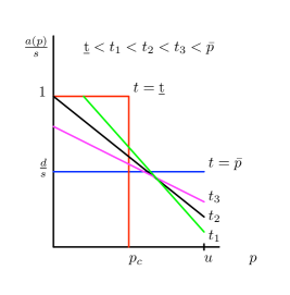
Figure 1: Effect of target spend on $L_{2}$-optimal allocation

2.2 Randomized bidding strategies

The quantity $a(p)/s$ is an optimal allocation, i.e., a recommendation to the publisher as to how much inventory to allocate to a guaranteed contract at every price $p$. However, recall that the publisher needs to acquire this inventory on behalf of the guaranteed contract by bidding in the spot market. The following theorem shows how to do this when ${\bf u}$ is the $L_{2}$ distance.

Theorem 1.

The optimal allocation for the $L_{2}$ distance measure can be implemented (in expectation) in an auction by the following random strategy: toss a coin to decide whether or not to bid, and if bidding, draw the bid from a uniform distribution.

Proof.

From (6) that the optimal allocation can be represented as

$$\frac{a(p)}{s}=\min\{1,z(p_{max}-p)\}.$$

By Proposition 1, an allocation $\frac{a(p)}{s}=\min\{1,z(p_{max}-p)\}$ can be implemented by bidding in an auction using the following randomized bidding strategy: with probability $\min\{zp_{\max},1\}$, place a bid drawn uniformly at random from the range $[\max\{p_{\max}-\frac{1}{z},0\},p_{\max}]$. ∎

The optimal allocation for KL-divergence decays exponentially with price, and the bidding strategy involves drawing bids from an exponential distribution; see Appendix C for details.

3 Multiple contracts

We now study the more realistic case where the publisher needs to fulfill multiple guaranteed contracts with different advertisers. Specifically, suppose there are $m$ advertisers, with demands $d_{j}$. As before, there are a total of $s\geq\sum d_{j}$ advertising opportunities available to the publisher. An allocation $a_{j}(p)/s$ is the proportion of opportunities purchased on behalf of contract $j$ at price $p$. Of course, the sum of these allocations cannot exceed 1 for any $p$, which corresponds to acquiring all the supply at that price.

As in the single contract case, we are first interested in what allocations $a_{j}(p)$ are implementable by bidding in an auction. However, in addition to being implementable, we would like allocations that satisfy an additional practical requirement, explained below. Notice that the publisher, acting as a bidding agent, now needs to acquire opportunities to implement the allocations for each of the guaranteed contracts. When an opportunity comes along, therefore, the publisher needs to decide which of the contracts (if any) will receive that opportunity. There are two ways to do this: the publisher submits one bid on behalf of all the contracts; if this bid wins, the publisher then selects one amongst the contracts to receive the opportunity. Alternatively, the publisher can submit one bid for each contract; the winning bid then automatically decides which contract receives the opportunity. We refer to the former as a centralized strategy and the latter as a decentralized strategy.

There are situations where the publisher will need to choose the winning advertiser prior to seeing the price, that is, the highest bid from the spot market. For example, to reduce latency in placing an advertisement, the auction mechanism may require that the bids be accompanied by the advertisement (or its unique identifier). A decentralized strategy automatically fulfills this requirement, since there is one bid for each contract and the highest bid wins, so that the choice of winning contract does not depend upon knowing the price. In a centralized strategy, this requirement means that the relative fractions won at price $p$, $a_{i}(p)/a_{j}(p)$, are independent of the price $p$– when this happens, the choice of advertiser can be made (by choosing at random with probability proportional to $a_{j}$) without knowing the price.

As before, we will be interested in implementing optimal (i.e., maximally representative) allocations. For such an allocation, as we will show in Section 3.2, if the relative fractions are independent of the price, they can also be decentralized. We will, therefore, concentrate on characterizing allocations which can be implemented via a decentralized strategy.

3.1 Decentralization

In this section, we examine what allocations can be implemented via a decentralized strategy. Note that it is not sufficient to simply use a distribution $H_{j}=1-\frac{a_{j}(p)}{a_{j}(0)}$ as in Proposition 1, since these contracts compete amongst each other as well. Specifically, using the distribution $1-\frac{a_{j}(p)}{a_{j}(0)}$ will lead to too few opportunities being purchased for contract $j$, since this distribution is designed to compete against $f$ alone, rather than against $f$ as well as the other contracts. We need to show how to choose distributions in such a way that lead to a fraction $a_{j}(p)/s$ of opportunities being purchased for contract $j$, for every $j=1,\ldots,m$.

First, we argue that a decentralized strategy with given distributions $H_{j}$ will lead to allocations that are non-increasing, as in the single contract case. A decentralized implementation uses distributions $H_{j}$ to bid for impressions, i.e., it draws a bid randomly from the distribution $H_{j}$ to place in the auction on behalf of $j$-th contract. Then, contract $j$ wins an impression at price $p$ with probability

$$a_{j}(p)=\int_{p}^{\infty}\left(\prod_{k\neq j}H_{k}(x)\right)h_{j}(x)dx,$$

since to win, the bid for contract $j$ must be larger than $p$ and larger than the bids placed by each of the remaining $m-1$ contracts. Since all the quantities in the integrand are nonnegative, $a_{j}$ is non-increasing in $p$.

Now assume that $a_{j}$ are differentiable almost everywhere (a.e.) and non-increasing. Let

$$\frac{A(p)}{s}:=\sum_{j}\frac{a_{j}(p)}{s}$$

be the total fraction of opportunities at price $p$ that the publisher needs to acquire. Clearly, $a_{j}$ must be such that $A(p)\leq s,~{}\forall p$. Let $p*:=\inf\{p:A(p)<s\}$. Now define

$$H_{j}(p):=\left\{\begin{array}[]{ll}e^{\int_{p}^{\infty}a^{\prime}_{j}(x)/(s-A(x))dx}&~{}~{}p>p^{*}\\ 0&~{}~{}{\rm\mbox{else}}\end{array}\right.$$ (7)

Then, $H_{j}(p)\geq 0$ and is continuous. Since $a_{j}^{\prime}(p)$ is non-increasing, $H_{j}(p)$ is monotone non-decreasing. Further, $H(\infty)=1$ and $H_{j}(p^{*})=0$. Thus, $H_{j}$ is a distribution function. Now we verify that bidding according to $H_{j}$ will result in the desired allocations: Note that

$$h_{j}(p)=\frac{d}{dp}H_{j}(p)=H_{j}(p)\frac{-a_{j}^{\prime}(p)}{s-A(p)}$$

which implies

$$\frac{A^{\prime}(p)}{s-A(p)}=\sum_{j}\frac{a^{\prime}_{j}(p)}{s-A(p)}=-\sum_{j}\frac{h_{j}(p)}{H_{j}(p)},$$

so that

$$-\log(s-A(x))|_{p}^{\infty} = \int_{p}^{\infty}\frac{A^{\prime}(x)}{s-A(x)}dx=-\int_{p}^{\infty}\sum_{j}\frac{h_{j}(x)}{H_{j}(x)}dx=-\sum_{j}\log(H_{j}(x))|_{p}^{\infty}$$

or

$$\log(s-A(p))=\sum_{j}\log(H_{j}(p))$$

and hence

$$\prod_{k}H_{k}(p)=s-A(p).$$

Then, the fraction of impressions at $p$ that are won by contract $j$ is

$$\int_{p}^{\infty}\left(\prod_{k\neq j}H_{k}(x)\right)h_{j}(x)dx=\int_{p}^{\infty}\left(\prod_{k}H_{k}(x)\right)\frac{h_{j}(x)}{H_{j}(x)}dx=\int_{p}^{\infty}(s-A(x))\frac{h_{j}(x)}{H_{j}(x)}dx=\int_{p}^{\infty}-a_{j}^{\prime}(x)dx~{}=~{}\frac{a_{j}(p)}{s}$$

Thus, we constructed distribution functions $H_{j}(p)$ which implement the given non-increasing (and a.e. differentiable) allocations $a_{j}(p)$. If any $a_{j}$ is increasing at any point, the set of campaigns cannot be decentralized. We summarize this in the following theorem, whose special case for the single contract case is Proposition 1:

Theorem 2.

A set of allocations $a_{j}(p)$ can be implemented in an auction via a decentralized strategy if and only if each $a_{j}(p)$ is non-increasing in $p$, and $\sum_{j}a_{j}(p)/s\leq 1$.

Having determined which allocations can be implemented by bidding in an auction in a decentralized fashion, we turn to the question of finding suitable allocations to implement. As in the single contract case, we would like to implement allocations that are maximally representative, given the spend constraints.

3.2 Optimal allocation for multiple contracts

As in the single contract case, every contract would ideally like an equal proportion of opportunities at every price. However, every contract has a per unit target spend which limits the fraction of opportunities that can be purchased at higher prices. In addition to the target spend, the allocation is also constrained by the fact that the total fraction of opportunities bought at every price must not exceed one. The maximally representative allocation is the allocation closest to the ideal allocation that satisfies the target spend constraints, and such that the collective allocation does not exceed the supply at any price. That is, it is the solution to the optimization problem below with the $L_{2}$ distance measure in the objective. We use $j$ to index the $m$ contracts.

$$\begin{array}[]{cl}\min&\frac{s}{2}\sum_{j=1}^{m}\int_{p}(\frac{a_{j}(p)}{s}-\frac{d_{j}}{s})^{2}f(p)dp\\[4.30554pt] \mbox{s.t.}&\int_{p}a_{j}(p)f(p)dp=d_{j}\qquad\forall j\\[4.30554pt] &\int_{p}pa_{j}(p)f(p)dp\leq t_{j}d\qquad\forall j\\[4.30554pt] &a_{j}(p)\geq 0\qquad\forall p,j\\[4.30554pt] &\sum_{j=1}^{m}a_{j}(p)\leq s\qquad\forall p\end{array}$$ (8)

Observe that the allocations for individual contracts are coupled only by the last constraint.

Optimality conditions: Introduce Lagrange multipliers $\lambda_{1}^{j}$ and $\lambda_{2}^{j}$ for the first and second constraints, and $\mu_{1}^{j}(p),\mu_{2}(p)$ for the last two inequalities. The optimality conditions are

$$\frac{a_{j}(p)}{s}-\frac{d_{j}}{s}=\lambda^{j}_{1}-\lambda^{j}_{2}p+\mu_{1}^{j}(p)-\mu_{2}(p),$$

where $\lambda_{2}^{j},\mu^{j}_{1}$ and $\mu_{2}$ must be nonnegative and can be non-zero only when the corresponding constraint is tight. Note that $\mu_{2}$ is a contract-independent multiplier, corresponding to the coupling constraint.

Suppose $a_{j}(p^{\prime})\geq 0~{}\forall j$ and $\sum_{j}a_{j}(p^{\prime})<s$ for some $p^{\prime}>0$. Then, $\mu_{1}^{j}(p^{\prime})=\mu_{2}(p^{\prime})=0$. It follows that for $p>p^{\prime}$, $a_{j}(p)<a_{j}(p^{\prime})$. Let $p^{*}=\inf~{}\{p:\sum_{j}a_{j}(p)<s\}$. Then, $\forall p\geq p^{*}$, each $a_{j}$ decays linearly with slope $\lambda_{2}^{j}$ until it becomes 0. If $p^{*}=0$, the solutions decouple, as $\mu_{2}(p)\equiv 0$. In this case, we can solve for the $a_{j}$s independently of one another. However, if $p^{*}>0$, we have $\forall p<p^{*}$:

$$\frac{a_{j}(p)}{s}-\frac{d_{j}}{s}=\lambda^{j}_{1}-\lambda^{j}_{2}p-\mu_{2}(p).$$

Together with $\sum_{j}a_{j}(p)=s$, this implies

$$-\mu_{2}(p)=\frac{1}{m}-\frac{1}{ms}\sum_{j}d_{j}-\frac{1}{m}\sum_{j}\lambda_{1}^{j}+p\frac{1}{m}\sum_{j}\lambda_{2}^{j}.$$

Denoting $\bar{\lambda_{2}}:=\frac{1}{m}\sum_{j}\lambda_{2}^{j}$, we see that

$$\frac{a_{j}(p)}{s}=c_{j}-(\lambda_{2}^{j}-\bar{\lambda_{2}})p,\qquad\forall p<p^{*}.$$

Therefore, at least one $a_{j}$ will have a positive slope below $p^{*}$ unless $\lambda_{2}^{j}=\lambda_{2}^{k},~{}\forall j,k$. That is, decentralization is not always guaranteed. In case the target spends are such that $p^{*}>0$ and $\lambda_{2}^{j}=\lambda_{2}^{k},~{}\forall j,k$, the optimal allocations $a_{j}$ stay flat until $p^{*}$ and then decay with identical slopes until each becomes 0, as shown in Figure 2.

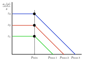
Figure 2: Coupled decentralizable allocation.

Thus, the optimal allocation is decentralizable in two cases:

1. $p^{*}=0~{}$: The target spends are such that the solutions decouple. In this case the allocation for each contract is independent of the others; we solve for the parameters of each allocation as in Section 2.1.1.

2. $p^{*}>0~{}$: The target spends are such that, for all $j,k,~{}\frac{a_{j}(p)}{a_{k}(p)}$ is independent of $p$. In this case we need to solve for the common slope and $p_{\min}$, and the contract specific values $p^{j}_{\max}$, which together determine the allocation. This can be done using, for instance, Newton’s method.

When the target spends are such that the allocation is not decentralizable, the vector of target spends can be increased to reach a decentralizable allocation. One way is to scale up the target spends uniformly until they are large enough to admit a separable solution; this has the advantage of preserving the relative ratios of target spends. The minimum multiplier which renders the allocation decentralizable can be found numerically, using for instance binary search.

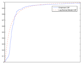
Figure 3: Empirical cumulative density function of the bids on the exchange and a log-normal fit to the distribution.

4 Experimental Validation

Our algorithms for obtaining representative allocations are randomized, and all of the results are derived in expectation. In this section we simulate the performance of the algorithms, and verify that the randomization does not lead to under-delivery for a realistic choice of bid landscape $f$.

To simulate the bid landscape, data was collected from live auctions conducted by the RightMedia exchange. RightMedia runs the largest spot market for display advertising, with billions of auctions daily. Winning bids were collected from approximately 400,000 auctions over the course of a day for a specific publisher. The cdf of the empirical bid distribution is plotted in Figure 3. (The scale on the x-axis is omitted for privacy concerns.)

The empirical distribution is well approximated by a log-normal distribution, as seen in Figure 3. For the experimental evaluation, we, therefore, draw bids from a log-normal distribution. The mean of the distribution is set to $0$, and the variance parameter is changed to investigate the sensitivity of our algorithms to the variance of the bid landscape.

To study the effectiveness of the algorithm in winning the right number of impressions on the exchange, we fix the target fraction, $\frac{d}{s}$ at $0.25,0.5$ and $0.75$, and compute the $p_{\max}$ necessary to achieve the allocation, yet minimize the total spend. For each setting of the variance of the exchange distribution, we run 15 trials, each with 10,000 auctions total. The results are plotted in Figure 4(a).

We perform a similar experiment to investigate the dependency of the target spend on the variance of the bid distribution. In this case, we fix the allocation fraction to $0.8$ and target spend to $0.25\mu$, $0.5\mu$ and $0.75\mu$, where $\mu=\int_{p}pf(p)dp$ is the maximum achievable target spend. For each setting of the variance parameter we run 15 trials each with 10,000 auctions. The results are plotted in Figure 4(b).

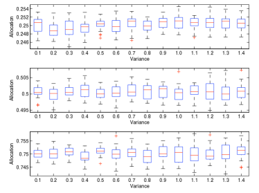
(a) Allocation achieved for different exchange distributions with ideal allocation of $0.25$, $0.5$ and $0.75$ fraction of the total.

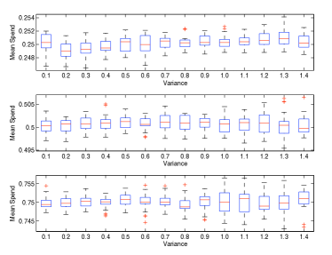
(b) Target spend achieved for different exchange distributions with ideal target $0.25$, $0.5$ and $0.75$ of the maximum feasible spend.

Figure 4: Experiment evaluation

In both simulations, the specific $p_{\min}$ and $p_{\max}$ for each variance setting vary greatly to achieve the desired allocation and target spend. However, the changes in the resulting $\frac{a}{s}$ and $\frac{d}{s}$ themselves are minimal – the algorithm rarely underdelivers or under/overspends by more than 1%; it is robust to variations in the variance of the underlying bid distributions.

5 Conclusion

Moving guaranteed contracts into an exchange environment presents a variety of challenges for a publisher. Randomized bidding is a useful compromise between minimizing the cost and maximizing the quality of guaranteed contracts. It is akin to the mutual fund strategy common in the capital asset pricing model. We provide a readily computable solution for synchronizing an arbitrary number of guaranteed campaigns in an exchange environment. Moreover, the solution we detail appears stable with real data.

There are many interesting directions for further research. We assumed throughout that the supply is known to the publisher. A more realistic model assumes either an unknown or a stochastic supply (a strawman solution is to use algorithms in this paper using a lower bound on the supply in place of $s$). Another interesting avenue is analyzing the strategic behavior by other bidders on the spot market in response to such randomized bidding strategies.

Appendix

Appendix A Solving for $p_{\min}$ and $p_{\max}$

Calling $p_{\min}$ and $p_{\max}$ $x$ and $y$ respectively, we want to solve the system of equations:

$$f(y,x)=\frac{d}{s}\left[\begin{array}[]{c}1\\ t\end{array}\right],$$

where

$$f(y,x)=\left[\begin{array}[]{c}F(x)+\int_{x}^{y}\frac{y-p}{p-x}f(p)dp\\[4.30554pt] \int_{0}^{x}pf(p)dp+\int_{x}^{y}p\frac{y-p}{y-x}f(p)dp\end{array}\right].$$

We will show that the derivative matrix is invertible so we can use Newton’s method to converge to the solution.

The derivative of f is:

$$f^{\prime} =\left[\begin{array}[]{cc}\int_{x}^{y}\frac{p-x}{(y-x)^{2}}f(p)dp&\int_{x}^{y}\frac{y-p}{(y-x)^{2}}f(p)dp\\[4.30554pt] \int_{x}^{y}p\frac{p-x}{(y-x)^{2}}f(p)dp&\int_{x}^{y}p\frac{y-p}{(y-x)^{2}}f(p)dp\end{array}\right]$$

$$=\frac{1}{(y-x)^{2}}\left[\begin{array}[]{cc}\int_{x}^{y}(p-x)f(p)dp&\int_{x}^{y}(y-p)f(p)dp\\[4.30554pt] \int_{x}^{y}p(p-x)f(p)dp&\int_{x}^{y}p(y-p)f(p)dp\end{array}\right]$$

$$=\frac{F(y)-F(x)}{(y-x)^{2}}\left[\begin{array}[]{cc}Ep-x&y-Ep\\[4.30554pt] E{p^{2}}-xEp&yEp-Ep^{2}\end{array}\right],$$

where we have defined $Ep=E[p|x\leq p\leq y]$.

It is easy to check that $Ep-x,y-Ep$ and $Ep^{2}-xEp$ are positive since $x\leq p\leq y$. For the final term, observe that $yEp-p^{2}=E(yp-p^{2})=Ep(y-p)\geq 0$. We note that $Ep^{2}=(Ep)^{2}+\sigma^{2}$ where $\sigma^{2}$ is the variance of $p$ conditioned on $x\leq p\leq y$, and therefore can compute the determinant to be $-(y-x)\sigma^{2}$.

Therefore, provided that $y>x$ and $F$ is non-degenerate, the matrix is invertible; which in turn implies that we can use Newton’s method to find the solution.

Appendix B Proof of Continuity – $L_{2}$

Given the (Lebesgue) integral in the objective, $a$ is not assumed continuous a priori. We show that the optimal solution, however, is. Let $t$ be the average target spend per unit.

$$\begin{array}[]{cl}\inf_{a(\cdot)}&\frac{s}{2}\int(\frac{a(p)}{s}-\frac{d}{s})^{2}~{}f(p)dp\\ \mbox{s.t.}&\int a(p)f(p)dp=d\\ &\int pa(p)f(p)dp\leq td\\ &0\leq\frac{a(p)}{s}\leq 1.\end{array}$$ (9)

We will ignore the nonnegativity constraint for simplicity. The Lagrangian is

$$L = \frac{1}{2s}\int\left(a(p)-d\right)^{2}~{}f(p)dp+\int\mu(p)[a(p)-s]f(p)dp$$

$$~{}~{}+~{}z\left(\int a(p)f(p)dp-d\right)$$

$$~{}~{}+~{}\lambda\left(\int pa(p)f(p)dp-td\right)$$

with $\mu(\cdot)\geq 0$ and $\lambda\geq 0$. Note that $\mu(p)=0$ if $a(p)<s$. By Euler-Lagrange,

$$\frac{a}{s}-\frac{d}{s}+\mu(p)+z+\lambda p=0$$

Then,

$$\int a(p)f(p)dp=d~{}\Rightarrow~{}z=\int(-\mu(p)-\lambda p)f(p)dp$$

and

$$a(p)=d-sz-s\mu(p)-s\lambda p~{}~{}~{}\forall p$$

Now suppose there is a $p^{\prime}$ such that $a(p^{\prime})<s$. Then, $\mu(p^{\prime})=0$ and

$$a(p^{\prime})=d-sz-s\lambda p^{\prime}<s$$

Then, for $p>p^{\prime}$, we have

$$a(p) = d-sz-s\lambda p-s\mu(p)$$

$$\leq d-sz-s\lambda p~{}~{}(\mbox{because}~{}\mu(p)\geq 0)$$

$$< d-sz-s\lambda p^{\prime}=a(p^{\prime})$$

Thus, $a(p)$ is monotone non-increasing.

Let

$$p_{0}:=\inf\{p\geq 0~{}:~{}a(p)<s\}$$

Note that $p_{0}\in[0,F^{-1}(d/s)]$. Then,

$$\begin{array}[]{llll}a(p)&=&s&p<p_{0}\\ &=&d-sz-s\lambda p&0\leq p_{0}\leq p\leq p_{m}\\ &=&0&p_{m}\leq p\end{array}$$

Here, $p_{m}$ is such that $d-sz-s\lambda p_{m}=0$. We now express $z$ in terms of $\lambda,p_{0},p_{m}$ rather than in $\lambda,\mu(\cdot)$:

$$z(\lambda,p_{0},p_{m})=\frac{sF(p_{0})+d(F(p_{m})-F(p_{0})-1)-s\int_{p_{0}}^{p_{m}}\lambda pf(p)dp}{s(F(p_{m})-F(p_{0}))}$$

Similarly for the Lagrangian:

$$L(\lambda,p_{0}) = \frac{(s-d)^{2}F(p_{0})}{2s}+\int_{0}^{p_{0}}\lambda psf(p)dp$$

$$\frac{1}{2s}\int_{p_{0}}^{p_{m}}[s^{2}z^{2}-s^{2}\lambda^{2}p^{2}+2s\lambda pd]f(p)dp$$

It can be verified that

$$\frac{\partial z}{\partial p_{0}}=\frac{f(p_{0})(s-a(p_{0}))}{s(F(p_{m})-F(p_{0}))}$$

$$\frac{\partial L}{\partial p_{0}}=\frac{f(p_{0})}{2s}(s-a(p_{0})^{2}\geq 0$$

We see that either the optimum with respect to $p_{0}$ is achieved on the boundary ($p_{0}=0$ or $p_{0}=F^{-1}(d/s)$) or that $a(p_{0})=s$ at the optimum. We are not interested in the trivial case $p_{0}=F^{-1}(d/s)$. We thus have two cases:

Case 1.

$$a(p)=d-sz-s\lambda p<s~{}~{}~{}~{}\forall p\geq 0$$

Case 2.

$$\begin{array}[]{llll}a(p)&=&s&p<p_{0}\\ &=&s(1+\lambda(p_{0}-p)&0\leq p_{0}\leq p\leq p_{m}\\ &=&0&p_{m}\leq p\end{array}$$

We could combine the two cases by allowing $p_{0}$ to be negative.

Appendix C KL divergence

We want to minimize the KL divergence between $a(p)f(p)/d$ and $f(p)$:

$$\int\frac{a(p)f(p)}{d}\log\frac{a(p)f(p)/d}{f(p)}dp~{}=~{}\int f(p)\frac{a(p)}{d}\log\frac{a(p)}{d}dp$$

which is equivalent to minimizing

$$\int f(p)a(p)\log a(p)dp$$

Given the (Lebesgue) integral in the objective, $a$ is not assumed continuous a priori. We show that the optimal solution, however, is. Let $t$ be the average target spend per unit. Thus we have

$$\begin{array}[]{cl}\inf_{a(\cdot)}&\int a(p)\log a(p)~{}f(p)dp\\ \mbox{s.t.}&\int a(p)f(p)dp=d\\ &\int pa(p)f(p)dp\leq td\\ &0\leq\frac{a(p)}{s}\leq 1.\end{array}$$ (10)

Here, $t$ is the average target spend per unit. For feasibility, $t\geq\underline{p}:=\int_{0}^{F^{-1}(d/s)}psf(p)dp$. If $t\geq\bar{p}:=\int_{0}^{\infty}pf(p)dp$, the optimal solution is $a(p)\equiv d$.

The Lagrangian is

$$L = \int a(p)\log a(p)~{}f(p)dp+\int\mu(p)[a(p)-s]f(p)dp$$

$$~{}~{}+~{}\gamma\left(\int a(p)f(p)dp-d\right)+\lambda\left(\int pa(p)f(p)dp-td\right)$$

with $\mu(\cdot)\geq 0$ and $\lambda\geq 0$. Note that $\mu(p)=0$ if $a(p)<s$. By Euler-Lagrange,

$$1+\log a+\mu(p)+\gamma+\lambda p=0$$

which gives

$$a=e^{-\gamma-1}e^{-\mu(p)-\lambda p}$$

Then,

$$\int a(p)f(p)dp=d~{}\Rightarrow~{}d=e^{-\gamma-1}\int e^{-\mu(p)-\lambda p}f(p)dp$$

which leads to

$$a(p)=\frac{d}{Z(\lambda,\mu(\cdot))}e^{-\mu(p)-\lambda p}~{}~{}~{}\forall p$$

Now suppose there is a $p^{\prime}$ such that $a(p^{\prime})<s$. Then, $\mu(p^{\prime})=0$ and

$$a(p^{\prime})=\frac{d}{z}e^{-\lambda p^{\prime}}<s$$

Then, for $p>p^{\prime}$, we have

$$a(p) = \frac{d}{z}e^{-\lambda p-\mu(p)}\leq\frac{d}{z}e^{-\lambda p}~{}~{}(\mbox{because}~{}\mu(p)\geq 0)$$

$$< \frac{d}{z}e^{-\lambda p^{\prime}}=a(p^{\prime})$$

Thus, $a(p)$ is monotone non-increasing.

Let

$$p_{0}:=\inf\{p\geq 0~{}:~{}a(p)<s\}$$

Note that $p_{0}\in[0,F^{-1}(d/s)]$. Then,

$$\begin{array}[]{llll}a(p)&=&s&p<p_{0}\\ &=&\frac{d}{z}e^{-\lambda p}&p\geq p_{0}\end{array}$$

We now express $z$ in terms of $\lambda,p_{0}$ rather than in $\lambda,\mu(\cdot)$:

$$z(\lambda,p_{0})=\frac{d\int_{p_{0}}^{\infty}e^{-\lambda p}f(p)dp}{d-sF(p_{0})}$$

Similarly for the Lagrangian:

$$L(\lambda,p_{0}) = F(p_{0})s\log s+\log\frac{d}{z(\lambda,p_{0})}\int_{p_{0}}^{\infty}a(p)f(p)dp$$

$$~{}~{}+~{}\lambda\int_{0}^{p_{0}}psf(p)dp-\lambda td$$

from which follows

$$\frac{\partial L}{\partial p_{0}}=-sf(p_{0})[\log\frac{a(p_{0})}{s}-\frac{a(p)}{s}+1]\geq 0$$

We see that either the optimum with respect to $p_{0}$ is achieved on the boundary ($p_{0}=0$ or $p_{0}=F^{-1}(d/s)$) or that $a(p_{0})=s$ at the optimum. We are not interested in the trivial case $p_{0}=F^{-1}(d/s)$.

We have two cases for the form of the solution in the KL case.

Case 1.

$$a(p)=\frac{d}{z(\lambda)}e^{-\lambda p}<s~{}~{}~{}~{}\forall p\geq 0$$

Case 2.

$$\begin{array}[]{llll}a(p)&=&s&p<p_{0}\\ &=&se^{\lambda(p_{0}-p)}&p\geq p_{0}\geq 0\end{array}$$

Figure 5 shows the effect of varying target spend on the optimal allocation.

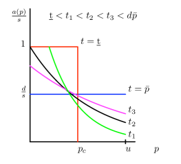
Figure 5: Effect of target spend on KL-optimal allocation

Parametric supply distributions As an illustration, we consider the case when the supply distribution $f$ is exponential: $f(p)=\gamma e^{-\gamma p}$. Note that $\bar{p}=\frac{1}{\gamma}$. As the budget decreases, a transition from Case 1 to Case 2 occurs at a certain budget. Until then, $a(p)=\frac{d}{z}e^{-\lambda p}$ where $\frac{d}{z}\leq s,$ with equality at the transitional budget. Demand constraint

$$\int\gamma\frac{d}{z}e^{-(\lambda+\gamma)p}dp=d$$

gives

$$z=\frac{\gamma}{\lambda+\gamma}$$

At the optimum, spend equals budget:

$$td=\int\gamma p\frac{d(\lambda+\gamma)}{\gamma}e^{-(\lambda+\gamma)p}dp=\frac{d}{\lambda+\gamma}$$

which leads to $\lambda_{*}=\frac{1}{t}-\gamma$ and $z=\gamma t$. Again, note that until the transition happens, $\frac{d}{\gamma t}\leq s$, that is, $t\geq\frac{d}{s\gamma}=\frac{d}{s}\bar{p}$. The optimal KL-divergence for $\frac{d}{s}\bar{p}\leq t\leq\bar{p}$ is given by

$$\mbox{KL}_{\mbox{\sc opt}}=\gamma t-1-\log\gamma t$$

which is 0 when $t=\bar{p}$ and is $\frac{d}{s}-1-\log\frac{d}{s}$ at the transitional budget.

References

- [1] Moshe Babaioff, Jason Hartline, and Robert Kleinberg. Selling banner ads: Online algorithms with buyback. In 4th Workshop on Ad Auctions, 2008.
- [2] C. Boutilier, D. Parkes, T. Sandholm, and W. Walsh. Expressive banner ad auctions and model-based online optimization for clearing. In National Conference on Artificial Intelligence (AAAI), 2008.
- [3] Florin Constantin, Jon Feldman, S Muthukrishnan, and Martin Pal. Online ad slotting with cancellations. In 4th Workshop on Ad Auctions, 2008.
- [4] I. Csiszar. Why least squares and maximum entropy? an axiomatic approach to interference for linear inverse problems. Annals of Statistics, 19(4):2032–2066, 1991.
- [5] Uriel Feige, Nicole Immorlica, Vahab S. Mirrokni, and Hamid Nazerzadeh. A combinatorial allocation mechanism with penalties for banner advertising. In Proceedings of ACM WWW, pages 169–178, 2008.
- [6] R. Preston McAfee and John McMillan. Auctions and bidding. Journal of Economic Literature, 25(2):699–738, 1987.
- [7] Paul R. Milgrom. A convergence theorem for competitive bidding with differential information. Econometrica, 47(3):679–688, May 1979.
- [8] David Parkes and Tuomas Sandholm. Optimize-and-dispatch architecture for expressive ad auctions. In 1st Workshop on Ad Auctions, 2005.
- [9] Tuomas Sandholm. Expressive commerce and its application to sourcing: How we conducted $35 billion of generalized combinatorial auctions. 28(3):45–58, 2007.
- [10] Robert Wilson. A bidding model of perfect competition. Rev. Econ. Stud., 44(3):511–518, 1977.