Diffuse continuum transfer in H ii regions

Abstract

We compare the accuracy of various methods for determining the transfer of the diffuse Lyman continuum in H ii regions, by comparing them with a high-resolution discrete-ordinate integration. We use these results to suggest how, in multidimensional dynamical simulations, the diffuse field may be treated with acceptable accuracy without requiring detailed transport solutions.

The angular distribution of the diffuse field derived from the numerical integration provides insight into the likely effects of the diffuse field for various material distributions.

1 Introduction

In this paper, we model the diffuse field structure of astrophysical H ii regions. Recombinations within these regions emit radiation in the various hydrogen line spectra and Balmer and higher continua which is an observed characteristic of them. Emission in the Lyman continuum, however, is energetic enough to ionize other hydrogen atoms, and so is trapped within the nebula. This radiation field is believed to have a significant fraction of the energy density of the direct ionizing continuum in some parts of the H ii region, and so it is important to model it correctly. This is particularly relevant when modelling the complex dynamics of the nebulae, or the emission from the internal features such as the tails of cometary globules in the Helix planetary nebula (O’Dell et al., 2007).

Ritzerveld (2005) has suggested that diffuse fields may be particularly important at the edges of H ii regions, in some regimes. This would seem to suggest that the diffuse field may have a more significant impact on their overall evolution than previously assumed. However, Ritzerveld uses a simple outward-only treatment of the diffuse radiation transport, and also assumes that the absorption coefficient is comparable for diffuse and direct radiation fields, although it is acknowledged that in reality the direct photons are likely to have a harder spectrum and will thus be significantly more penetrating.

To investigate the validity of these conclusions, in this paper we apply detailed discrete-ordinate angular integration to investigate the validity of several approximate numerical transport schemes. To simplify the problem, we assume a pure-hydrogen nebula, without dust, and use a simple two-frequency approximation to the radiation flow.

With our more detailed modelling, we find that the diffuse field can indeed dominate for the situations Ritzerveld describes. However, where the diffuse field dominates, it will typically also be outwardly-beamed and therefore be indistinguishable from the direct field for most purposes. For most astrophysically relevant conditions, the usual on-the-spot approximation is shown to give accurate results through most of a spherical nebula, except for a region close to the star where it overestimates the diffuse field.

We also assess the accuracy of the Eddington diffusion approximation for the diffuse field transfer, which may be a useful means of modelling diffuse transport effects in multidimensional simulations.

In the present paper, we neglect the effects of dust and heavy elements in the H ii region. This is a reasonable assumption for the case of cosmological H ii regions; however, there is observational evidence for the importance of dust absorption within the ionized gas in galactic H ii regions (Cesarsky et al., 2000; Robberto et al., 2005). We briefly discuss the impact dust might have on our results.

2 Governing equations and physical conditions

We use a simple model of H ii regions to study the diffuse field structure. We consider steady, spherically symmetric pure-hydrogen regions, with the radiation field in two frequency components: higher frequency radiation propagating directly from a central point source, and lower frequency diffuse radiation. We assume that the material within the H ii region is maintained at a constant temperature in ionization equilibrium.

In the absence of dust, the governing equations are then

$${dL_{\rm dir}/dr} = -n(1-x)a_{0}L_{\rm dir}$$ (1)

$${dI_{\rm dif}/ds} = -n(1-x)a_{1}I_{\rm dif}+{\alpha_{1}\over 4\pi}n^{2}x^{2}$$ (2)

$$\alpha_{\rm A}n^{2}x^{2} = n(1-x)\left({a_{0}L_{\rm dir}\over 4\pi r^{2}}+a_{1}\int I_{\rm dif}(r,\Omega^{\prime}){\,d\Omega^{\prime}}\right),$$ (3)

corresponding to the transfer of direct radiation from a point source, $L_{\rm dir}$, the diffuse radiation field $I_{\rm dif}(r,\theta)$, and balance of ionization and recombination for ionization fraction $x$. Here $L$ is the specific luminosity and $I$ the radiation intensity specified in terms of the number of photons, rather than the radiation energy, as this is more natural in the present application.

Integrating equations (1)–(3) over volume, and angle where appropriate, and applying the boundary conditions $L_{\rm dir}=L_{\star}$ at $r=0$, $I_{\rm dif}=0$ as $r\to\infty$, we find that

$$L_{\star}=\int\alpha_{\rm B}n^{2}x^{2}dV,$$ (4)

where $\alpha_{\rm B}=\alpha_{\rm A}-\alpha_{1}$. This has a simple interpretation, in that the number of ionizing photons into the nebula balances the number of recombinations which destroy such photons (rather than re-emitting a Lyman continuum photon).

If the ionization front is thin, as is typically the case, then a characteristic Strömgren radius for a spherical H ii region, $r_{\rm S}$, is given by

$$L_{\star}=\int_{0}^{r_{\rm S}}\alpha_{\rm B}n^{2}4\pi r^{2}dr,$$ (5)

independent of diffuse radiation transport effects.

From Osterbrock and Ferland (2006), we take values of the recombination coefficients at $10^{4}{\rm\,K}$ of $\alpha_{\rm A}=4.18\times 10^{-13}{\rm\,cm^{3}\,s^{-1}}$ and $\alpha_{\rm 1}=1.58\times 10^{-13}{\rm\,cm^{3}\,s^{-1}}$. We assume that the ionization cross section for the diffuse radiation is the Lyman limit cross section $a_{1}=6\times 10^{-18}{\rm\,cm^{2}}$, while for the direct photons, we take either $a_{0}=1\times 10^{-18}{\rm\,cm^{2}}$ (which allows for the largest likely effect of the higher average frequency of the direct photons) or $a_{0}=6\times 10^{-18}{\rm\,cm^{2}}$ (corresponding to the case which was primarily considered by Ritzerveld, 2005). In practice, the effective absorption coefficients will depend on the spectrum of the star and the recombination continuum, and their modification due to intervening absorption processes: the uncertainty is enhanced by the sharp dependence of the absorption cross section on the photon frequency above threshold (see Figure 2.2 in Osterbrock and Ferland, 2006).

The calculations are normalized to a star emitting ionizing photons at a rate $10^{48}{\rm\,s^{-1}}$, generating an equilibrium Strömgren sphere of radius $r_{\rm S}=1{\rm\,pc}$ in all cases. This corresponds to a density of $n_{\rm H}=n_{\rm e}=180{\rm\,cm^{-3}}$ for the uniform density case.

For direct comparison to Ritzerveld’s work, we consider three main density distributions: uniform, and proportional to $r^{-1}$ or $r^{-2}$ beyond an empty core of radius $10^{-6}\times r_{\rm S}$ and $0.05\times r_{\rm S}$, respectively.

3 Solution methods

3.1 OTS and the diffusion limit

The simplest approximation widely used in astrophysics is the case B approximation. Here, the diffuse field is assumed to be absorbed at the same point as it is emitted, so equation (2) is replaced by the on-the-spot (OTS) approximation

$$n(1-x)a_{1}I_{\rm dif}={\alpha_{1}\over 4\pi}n^{2}x^{2}.$$ (6)

Note that the diffuse radiation intensity is isotropic in this approximation. With this assumption, equation (3) simplifies to

$$\alpha_{\rm B}n^{2}x^{2}={n(1-x)a_{0}L_{\rm dir}\over 4\pi r^{2}},$$ (7)

and so

$${dL_{\rm dir}/dr}=-4\pi r^{2}\alpha_{\rm B}n^{2}x^{2}.$$ (8)

Since the hydrogen ionization fraction is close to unity through most of an astrophysical H ii region, this equation may then be integrated to define the Strömgren radius, in agreement with equation (5). The ratio of the diffuse field photon density to that of the ionizing field is

$$f_{\rm dif,OTS}={\int I_{\rm dif}d\Omega\over L_{\rm dir}/4\pi r^{2}}={\alpha_{1}a_{0}\over\alpha_{B}a_{1}},$$ (9)

which is roughly $60$ per cent for equal absorption cross sections, or $\sim 10$ per cent if we assume a lower absorption cross section for direct photons. The ratio of the diffuse flux through a surface (of any orientation) to the direct flux through a surface directed towards the star will be one quarter of this value (as in the analysis of Cantó et al., 1998, who assume $a_{0}=a_{1}$, and thus find $F_{\rm D}=0.15F_{\star}$).

If we wish to extend this analysis, we need to obtain a better estimate for $J_{\rm dif}=\int I_{\rm dif}d\Omega$ to insert in equation (3). Writing equation (2) as

$${dI_{\rm dif}\over ds}=-\kappa I_{\rm dif}+{\epsilon\over 4\pi},$$ (10)

where $\kappa=n(1-x)a_{1}$ is the opacity and $\epsilon=\alpha_{1}n^{2}x^{2}$ is the volume emissivity, then we can write

$$J_{\rm dif}={\epsilon\over\kappa}-{1\over\kappa}\int d\Omega{dI_{\rm dif}\over ds}$$ (11)

This exact expression remains dependent on $I_{\rm dif}$. If we apply the on-the-spot approximation $I_{\rm dif}\simeq\epsilon/4\pi\kappa$ to truncate the hierarchy at this approximation, the integration over angle is zero, which shows that the case B approximation is accurate to second order.

To obtain more accurate results, however, we can substitute for $I_{\rm dif}$ again using equation (10). This gives

$$J_{\rm dif}={\epsilon\over\kappa}+{1\over\kappa}\int{d\over ds}\left({1\over\kappa}{dI_{\rm dif}\over ds}-{\epsilon\over 4\pi\kappa}\right)d\Omega.$$ (12)

Again, the second term in the integral will be zero. Assuming the remaining $I_{\rm dif}$ term is also isotropic to first order, it will be a function of radius alone, so

$${dI_{\rm dif}\over ds} = \cos\theta{dI_{\rm dif}\over dr}$$ (13)

$${d\over ds}\left({1\over\kappa}{dI_{\rm dif}\over ds}\right) = \cos^{2}\theta{d\over dr}\left({1\over\kappa}{dI_{\rm dif}\over dr}\right)+\sin^{2}\theta{1\over\kappa r}{dI_{\rm dif}\over dr}$$ (14)

and so

$$J_{\rm dif}\simeq{\epsilon\over\kappa}+{1\over\kappa r^{2}}{d\over dr}{r^{2}\over 3\kappa}{dJ_{\rm dif}\over dr},$$ (15)

corresponding to Eddington approximation $J=3K$ (e.g. Mihalas & Weibel-Mihalas, 1999). Thus given a distribution of ionization, we can solve for the diffuse field using this expression, in which the diffusive transport corrects the OTS intensity. Note, that since $x\sim 1$ in the centre of the H ii region, the free path $1/\kappa$ may be large.

3.2 Ritzerveld’s outward-only approximation

Ritzerveld (2005) solves an outward-only system

$${dL_{\rm dir}\over dr} = -\xi\alpha_{\rm A}n^{2}r^{d-1}{cL_{\rm dir}\over cL_{\rm dir}+L_{\rm dif}}$$ (16)

$${dL_{\rm dif}\over dr} = -\xi\alpha_{\rm A}n^{2}r^{d-1}{L_{\rm dif}\over cL_{\rm dir}+L_{\rm dif}}+\xi r^{d-1}\alpha_{1}n^{2},$$ (17)

where for slab symmetry $d=1$, $\xi=1$, for cylindrical symmetry $d=2$, $\xi=2\pi$ and for spherical symmetry $d=3$, $\xi=4\pi$. Note that these equations are given here for the total ionization intensity integrated over the surface at the specified radius. Ritzerveld states that they apply to the density of photons per unit volume, but this is clearly not the case, as if all the recombination coefficients are zero, then $L_{\rm dir}=L_{\rm dif}={\it const}$. This system approximates the transport in the limit of nearly complete ionization within the H ii region. The factor $c=a_{0}/a_{1}$ allows for the preferential absorption of the diffuse photons.

The results presented by Ritzerveld (2005) can be generalized to the case of arbitrary ratios of absorption cross section. Adding equations (16) and (17), we find

$${d\over dr}\left(L_{\rm dir}+L_{\rm dif}\right)=-\xi\alpha_{\rm B}n^{2}r^{d-1},$$ (18)

and hence

$$L_{\rm tot}\equiv L_{\rm dir}+L_{\rm dif}=L_{\star}-\int^{r}\xi\alpha_{\rm B}n^{2}r^{d-1}dr.$$ (19)

A general (implicit) expression for the direct and diffuse fields can be derived in terms of the total field, independent of the density distribution or geometry. Dividing equation (18) by equation (16), we find

$${dL_{\rm tot}\over dL_{\rm dir}}={\alpha_{\rm B}\over c\alpha_{\rm A}}\left({L_{\rm tot}\over L_{\rm dir}}+c-1\right),$$ (20)

and hence

$$L_{\rm tot}={1\over\alpha_{\rm A}c-\alpha_{\rm B}}\left[\alpha_{1}cL_{\star}\left(L_{\rm dir}\over L_{\star}\right)^{\alpha_{\rm B}/c\alpha_{\rm A}}-(1-c)\alpha_{\rm B}L_{\rm dir}\right].$$ (21)

Given $L_{\rm tot}(r)$ from equation (19) above, equation (21) may then be solved for $L_{\rm dir}$ (explicitly in the case $c=1$, to recover the analytic solutions which Ritzerveld presents), and then $L_{\rm dif}=L_{\rm tot}-L_{\rm dir}$.

3.3 Full transfer

We use an iterative technique to find solutions, using similar techniques to those applied elsewhere (Hummer & Seaton, 1963; Rubin, 1968). Here, we integrate the diffuse field using a large number of coaxial zones.

We first derive an approximate ionization structure using the case B approximation, and use this to estimate the outward-going diffuse field components. We integrate the diffuse field transport inwards through this structure. As part of this sweep, we calculate an improved estimate for the ionization structure taking account of the new inward radiation field beams. We then integrate the direct radiation and outward-going diffuse field outward through the resulting structure, using the inward diffuse field at its closest point to the star as the initial condition for the outward beams, updating the ionization structure again. We iterate these inward and outward sweeps until the ionization structure has converged – this convergence is rapid in practice.

The results for the ionization structure are very sensitive to the details of the numerical scheme for the case where the density varies as $r^{-2}$, in particular the Strömgren radius can vary significantly. As noted by Franco et al. (1990), the ionization front can in this case escape to infinity: having the ionization front at 20 times the inner radius of the density distribution requires a rather precisely tuned value of the incident radiation field. This feeds through to the numerical sensitivity.

As a result of this, considerable care has to be taken in the radiation field integration to ensure the rate at which photons are removed from the radiation field is consistent with the ionization rate within the zone (Abel et al., 1999; Williams, 2002; Mellema et al., 2006; Whalen & Norman, 2006). To do this, we will adapt the approach described by Williams (2002) to the case of multiple incident beams of radiation and diffuse sources.

We specify the radiation field in coaxial cylindrical zones, which intersect spherical shells within which the physical variables are assumed to be uniform. We take the $i$-th component of the density field to occupy a spherical shell of outer radius $r_{i}=i\Delta$, and the $j$-th group of diffuse photons to be those with an impact parameter between $R_{j-1}$ and $R_{j}$, where $R_{j}=j\Delta$.

Integrating equation (3) over a spatial zone, we have

$$\alpha_{\rm A}n^{2}x^{2}\Delta V_{i} = \int_{r_{i-1}}^{r_{i}}n(1-x)\left({a_{0}L_{\rm dir}\over 4\pi r^{2}}\right.+$$ (22)

$$\quad\left.a_{1}\int I_{\rm dif}(r,\Omega^{\prime}){\,d\Omega^{\prime}}\right)\,dV,$$

where

$$\Delta V_{i}={4\pi\over 3}\left(r_{i}^{3}-r_{i-1}^{3}\right).$$ (23)

Substituting from the transport equations, (1) and (2), then gives

$$\alpha_{\rm B}n^{2}x^{2}\Delta V_{i} = -\left[L_{\rm dir}\right]_{r_{i-1}}^{r_{i}}$$ (24)

$$\quad-\int_{r_{i-1}}^{r_{i}}\int{dI_{\rm dif}\over ds}\,d\Omega^{\prime}4\pi r^{2}\,dr,$$

where the problem is uniform in space, so the angular integral over the zone volume is trivial. Combining the spatial integral $r^{2}dr$ with the beam solid angle integral $d\Omega^{\prime}$, however, yields an integral which may be taken as over the zone volume for beams which are incident from a single direction. This may be discretized as the difference in diffuse flux within each radiation bin across the zone,

$$\int_{r_{i-1}}^{r_{i}}\int{dI_{\rm dif}\over ds}\,d\Omega^{\prime}4\pi r^{2}\,dr=\int_{\Omega_{i}}{dI_{\rm dif}\over ds}(b,s)4\pi\cdot 2\pi b\,db\,ds,$$ (25)

where the integral may now be approximated as the change in the diffuse flux within the cylinder

$$I_{{\rm dif},j}\Delta A_{j} = \int_{b_{j-1}}^{b_{j}}I_{\rm dif}2\pi b\,db$$ (26)

$$\int_{s_{i-1}}^{s_{i}}{dI_{\rm dif}\over ds}ds = I_{\rm dif,\it i}-I_{\rm dif,\it i-1}$$ (27)

as the photons pass across the radial zone. Again, this has the interpretation that the difference between ionizing photons into and out of the zone is balanced with the rate of recombinations in the zone which destroy such photons.

In order to evaluate the differences in the direct and diffuse fluxes on either side of the zone, we discretize the transport equations. There are a range of choices for this discretization, which give different forms for the equations to be solved to evaluate the ionization fraction (Williams, 2002).

As the source function from the recombinations means that there is no simple closed form solution to the ionization equilibrium problem in the zone, we instead choose a scheme where the outgoing beams are guaranteed to be positive. We integrate the transfer equation (2) across a uniform zone to give

$$I(s+\Delta s) \simeq I(s)\exp\left[-n(1-x)a_{1}\Delta s\right]+$$ (28)

$$\quad S_{\rm dif}(x)\left(1-\exp\left[-na_{1}(1-x)\Delta s\right]\right),$$

where

$$S_{\rm dif}(x)={\alpha_{1}nx^{2}\over 4\pi a_{1}(1-x)}$$ (29)

is the diffuse field source function. The change in ionizing flux across the zone required for the ionization balance equation in the form (24) is then

$$I(s+\Delta s)-I(s) = \left[S_{\rm dif}(x)-I(s)\right]\times$$ (30)

$$\quad\left(1-\exp\left[-n(1-x)a_{1}\Delta s\right]\right).$$

This expression must then be integrated over the cylindrical zone of impact parameters and the solid angle of photon directions to obtain a finite difference in the form needed to be used in equation (24). On the right hand side, we make the first-order assumption that a single mean path length applies to all photons within the photon zone as they cross the radial zone.

In order to perform the discrete integrals, we need to determine the volume of intersection between the radiation and spatial zones. The volume between these cylindrical and spherical shells, each of thickness $\Delta$, is contained in two disjoint components, apart from the case $i=j$. The radiation field in the latter case can still be advanced by the same formalism by splitting the zone in two at the intersection of the radiation beam with the equatorial plane. Note, however, that the additional radiation flux values introduced into the diffuse field arrays as a result must not be included when calculating radiation field moments at the radial zone interfaces.

Each component has volume

$$v_{i,j}={1\over 2}\left(V_{i-1,j}+V_{i,j-1}-V_{i,j}-V_{i-1,j-1}\right),$$ (31)

where $V_{i,j}$ is the volume within a coaxial sphere of radius $r_{i}$ but outside a cylinder of radius $R_{j}<r_{i}$,

$$V_{i,j}={4\pi\over 3}\left(r_{i}^{2}-R_{j}^{2}\right)^{3/2}.$$ (32)

The area of the cylindrical shell is

$$a_{j}=\pi(R_{j}^{2}-R_{j-1}^{2})=(2j-1)\pi\Delta^{2}.$$ (33)

Hence the average path length of photons within the cylindrical shell $j$ through one of the the intersections with the spherical shell is

$$\Delta s_{i,j}={v_{i,j}\over a_{j}}.$$ (34)

We use these distances as the chord lengths for propagation of the diffuse radiation propagation in the cylindrical shell labelled $j$ through its intersection with the spherical shell labelled $i$ in the ionization equilibrium solution, in order to obtain volume consistency. The resulting expression for the zone ionization, including all direct and diffuse beams, is solved using Newton-Raphson iteration.

In all cases, we verify that at convergence the number of case B recombinations within the modelled H ii region balances the incoming ionizing flux to high accuracy.

4 Results

Figure 1: H ii region structures. Left column, with equal absorption coefficients, right column with diffuse coefficient 6 times direct. Top row uniform density, second row $r^{-1}$ outside a small core, last row $r^{-2}$ outside 0.05 core. Solid line is ionization fraction for full transfer solution, dotted is ionization fraction for OTS solution – in almost all cases, the ionization fractions are essentially identical. The lower panel in the plots shows $x_{\rm full}-x_{\rm OTS}$, with the scale set to show differences internal to the H ii region.

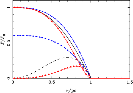
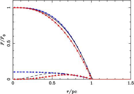
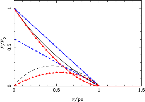
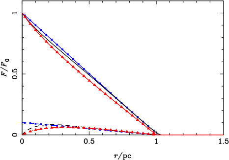
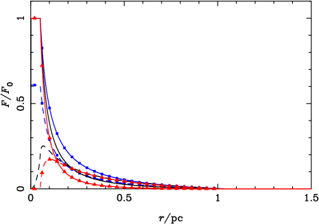
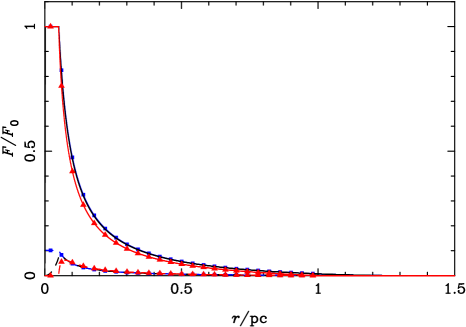
Figure 2: H ii region structures. Left column, with equal absorption coefficients, right column with diffuse coefficient 6 times direct. Top row uniform density, second row $r^{-1}$ outside a small core, last row $r^{-2}$ outside 0.05 core. Solid is direct photon rate, dashed is $4\pi r^{2}$ times the local diffuse intensity. OTS results have square markers, the approximation of Ritzerveld (2005) has triangular markers; the detailed transfer solution is plain. In general, the exact results lie between the two approximations; in lower right plot, the OTS and exact results are closely coincident.

Figure 3: Polar diagrams for the radiation at $0.1$ (solid), $0.5$ (dashed), $0.8$ (dot-dashed) and $0.9$ (dotted) $\times r_{\rm S}$. Left column, with equal absorption coefficients, right column with diffuse absorption coefficient 6 times that for direct photons. Top row uniform density, second row $r^{-1}$ outside a small core, last row $r^{-2}$ outside 0.05 core.

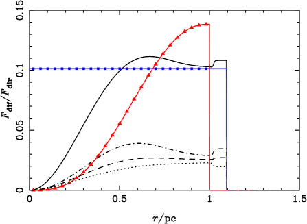
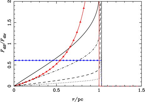
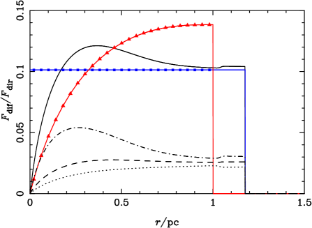
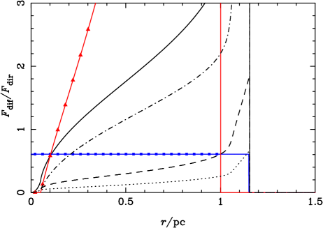
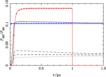
Figure 4: Diffuse field components as a fraction of the direct field for the full-transfer solution. Left column, with equal absorption coefficients, right column with diffuse coefficient 6 times direct. Top row uniform density, second row $r^{-1}$ outside a small core, last row $r^{-2}$ outside 0.05 core. Solid is the total diffuse energy density, dashed is the flux incident tangentially, dot-dashed is the outward flux, dotted is the inward flux. Square and triangular markers on solid lines show the total diffuse energy density estimated by the OTS and Ritzerveld approximations, respectively.

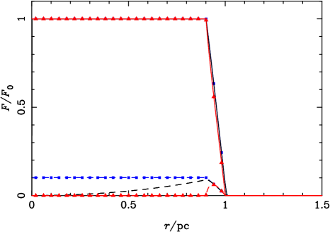
Figure 5: H ii region structure and polar diagram for a thin shell with zero density out to 90 per cent of the Strömgren radius and uniform density beyond. Left column, with equal absorption coefficients, right column with diffuse absorption coefficient 6 times direct. The line style and colours of the curves have the same meanings as defined in previous figures.

In this section, we present the results of the diffuse radiation solutions using a variety of numerical schemes, compared to the full transfer solutions. The full transfer solutions have been discretized on a grid with spatial resolution of $\Delta=0.001r_{\rm S}$ out to $2r_{\rm S}$.

In Figure 1, we show the ionization fraction structures for the OTS and exact transfer solutions. These are seen to be very close to each other in all cases, excpet for close to the ionization front, particularly in the case of equal absorption coefficients. In the case of an $r^{-2}$ density distribution, the outer edge of the H ii region is significantly broader. This is true for both the OTS and the full transfer solutions. The structure of the outer region of the ionized bubble in the $r^{-2}$ case is highly sensitive to details of the internal structure, as can be seen from the relation

$$L_{\star}=4\pi\alpha_{\rm B}n_{\rm c}^{2}r_{\rm c}^{4}(r_{\rm c}^{-1}-r_{\rm S}^{-1}),$$ (35)

so discretization errors at the 1 per cent level lead to changes in the outer radius of the ionized bubble $r_{\rm S}/r_{\rm c}$ times greater, i.e. 20 per cent for the parameters chosen by Ritzerveld (2005). In reality, it is likely that the ionized region would either be trapped in the core of the density distribution or extend to infinity; if the static solution were to be found in a region of such rapidly decreasing density, it is likely that the high sensitivity in its position would result in dynamical instability.

In Figure 2 we show the direct and diffuse radiation intensities. As expected, the diffuse field intensity is higher in the case of equal absorption coefficients. Overall, the complete integration gives results roughly intermediate between the OTS and Ritzerveld approximations.

The OTS approximation overestimates the diffuse field intensity in the core of the nebula, while the Ritzerveld approximation underestimates this. The direct field in the outer part of the nebula is reduced in the outer parts of the nebula in the Ritzerveld approximation, primarily as a result of the lower ionization in the core. For the case of $r^{-2}$, the assumption that $x=1$ within the Strömgren sphere means that this approximation also does not capture the broadening of the ionization front.

In Figure 3, we show the angular distribution of the diffuse radiation at various positions within the nebula. Where the absorption coefficients of direct and diffuse radiation are the same, the diffuse radiation field is also beamed strongly forward through much of the nebula, because it is principally emitted in the dense gas in the core. Hence, although the radiation energy may be distributed with the form characteristic of recombination emission, effects of a directed radiation field such as shadowing should still be in evidence. For the uniform density case with diffuse absorption coefficient six time larger than direct, the radiation field is most strongly beamed at intermediate radii within the nebula: the directionality is small at $r=0.1{\rm\,pc}$ for both uniform density cases as this is close to the centre of symmetry, where as for the higher absorption case the diffuse field is also symmetric near to the edge of the nebula because the $\tau_{\rm dif}\sim 1$ surface samples a relatively small degree of anisotropy in the direct field.

For the innermost radius of the $r^{-2}$ distribution with the higher absorption coefficient for the direct field, the inner edge of the photoionized gas can be clearly seen in the diffuse radiation field.

In Figure 4, we plot the diffuse radiation intensity as a fraction of the direct radiation intensity as a function of radius for our standard set of parameters. These results complement the polar diagrams at specific radii shown in Figure 3. As we have seen, in the case of equal absorption coefficients, the diffuse intensity can be higher than the direct intensity. However the ratio of the lateral diffuse flux to the direct flux, relevant to the illumination of the tails of cometary globules, reaches at most 60 per cent at the edge of a $r^{-2}$ density distribution, and through most of the nebula is closer to the 15 per cent figure derived by Cantó et al. (1998). In the case where the direct flux is less strongly absorbed, all the diffuse flux components are close to 2.5 per cent of the direct flux through almost all of the region; the outward-going flux shows the most structure, but only reaches at most around 5.5 per cent of the direct flux at its maximum.

This plot also shows the ratio of the diffuse to direct field in the OTS and Ritzerveld approximations. It is clear that the OTS approximation predicts a reasonable average value for this ratio, but overestimates the relative importance of the diffuse field in the core of the nebula and underestimates it at the edge of the nebula. In contrast, Ritzerveld’s formalism underestimates relative importance of the diffuse field in the core but overestimates it at the edge of the nebula, particularly for the case of equal absorption coefficients and steeply decreasing density distibutions (as we saw in Figure 2, this is primarily due to underestimating the direct field here). In both cases, the first approximation would be that the lateral diffuse field was one quarter the radiation intensity, which would be a significant overestimate for the case of equal absorption coefficients.

In Figure 5, we show the same results as previously for a thin shell of uniform density between $0.9r_{\rm S}$ and $r_{\rm S}$. In this case, Ritzerveld’s approximation obviously underestimates the diffuse field dramatically in the empty core of the nebula, as there are no recombinations in this region, while the OTS approximation overestimates the diffuse flux. The radiation field is symmetric in angle at all our sample points, which are at radii less than the inner edge of the shell: this is to be expected, as the angle to the surface from oppositely directed beams is the same and the surface brightness is constant. Particularly in the case with higher direct absorption coefficient, limb-brightening is seen for the sample point at the inner surface of the shell, corresponding to the higher direct flux (and hence source function) at the $\tau_{\rm dif}=1$ surface in this direction.

4.1 Transfer using the diffusion approximation

Figure 6: Accuracy of diffuse field determination for uniform density field. Left column, with equal absorption coefficients, right column with diffuse absorption coefficient 6 times that for direct photons. Solid line – ionization fraction; dotted line – OTS diffuse field divided by detailed transport diffuse field; dashed line – diffusion approximation diffuse field divided by detailed transport diffuse field.

In Figure 6, we compare the accuracy of a diffusion approximation solution to the diffuse field intensity to that of the on-the-spot approximation. The diffusion results are almost everywhere more accurate than the OTS approximation, being in error by less than 30 per cent even in the most difficult, central region of the flow. Both schemes are accurate at the edge of the nebula, where the most interesting dynamical structures occur, although the diffusion results are still significantly more precise.

A diffusion approximation solver could be embedded in a dynamical code by updating the ionization solution consistently with the sources derived from the diffusion solver and iterating, in a similar fashion to that which we use for the full field transfer. Experimenting with updating the ionization structure after both inward and outward transfer are complete suggests that the solution converges more slowly than if the ionization structure is updated on each sweep. However, in the context of a dynamical scheme, the initial approximation for the ionization structure will have come from the previous timestep, and hence would be expected to not be far from the correct solution.

The diffusion approximation allows processes such as the lateral illumination of the tails of photoionized globules to be modelled (Cantó et al., 1998; Pavlakis et al., 2001). However, the lateral illumination of shadowed tails may be overstimated in cases where the beaming of the diffuse field is expected to be strong (Mellema et al., 2006): Eddington tensor approaches (e.g. González & Audit, 2005) may improve the results in such limits.

5 Discussion

5.1 Accuracy of the OTS approximation

Figure 7: Functional dependence from equation (43) for power-law density indexes $m=0$ (solid), $m=1$ (dashed), $m=2$ (dot-dashed). This function shows where the OTS approximation for the diffuse field is expected to be accurate (roughly for radii where the ordinate is less than $a_{1}/a_{0}$).

The accuracy of the OTS approximation may be evaluated by comparing the scale of variation of the diffuse field source function, $H$, to the mean free path for diffuse photons, $\lambda=1/n(1-x)a_{1}$.

Using equation (29) for the source function, and the OTS approximation equation (7) for the ionization balance

$$S_{\rm dif}\simeq{1\over 4\pi}{\alpha_{1}a_{0}\over\alpha_{\rm B}a_{1}}{L_{\rm dir}\over 4\pi r^{2}}.$$ (36)

Note that we can still use the OTS approximation to close our equations at this higher order. The source function varies radially, so that

$$H^{-1} = \left|{1\over S_{\rm dif}}{dS_{\rm dif}\over dr}\right|$$ (37)

$$\simeq \left|{1\over L_{\rm dir}}{dL_{\rm dir}\over dr}-{2\over r}\right|$$ (38)

$$\simeq {4\pi r^{2}\alpha_{\rm B}n^{2}x^{2}\over L_{\rm dir}}+{2\over r},$$ (39)

where we have used equation (8). Now through most of the H ii region, $x\sim 1$, and hence

$$L_{\rm dir}\simeq{4\pi r^{2}\alpha_{\rm B}n^{2}x^{2}\over n(1-x)a_{0}}={a_{1}\over a_{0}}4\pi r^{2}\alpha_{\rm B}n^{2}\lambda,$$ (40)

and so

$${\lambda\over H} \simeq {a_{0}\over a_{1}}\left(1+{L_{\rm dir}\over 2\pi r^{3}\alpha_{\rm B}n^{2}}\right)$$ (41)

$$\simeq {a_{0}\over a_{1}}\left(1+{2\over n^{2}r^{3}}\int_{r}^{r_{\rm S}}n^{2}r^{2}dr\right),$$ (42)

where the integral is the result of equation (8). For a density distribution $n\propto r^{-m}$ outside some specific radius,

$${\lambda\over H}\simeq{a_{0}\over a_{1}}{1\over 3-2m}\left(2(r/r_{\rm S})^{2m-3}+1-2m\right)$$ (43)

(so long as $m\neq 3/2$). In Figure 7 we show the form of the r.h.s. of equation (43) for $a_{0}=a_{1}$. This suggests that OTS approximation will be most accurate close to the outer edge of H ii regions. When $a_{0}=a_{1}$, the OTS approximation for the diffuse field is only marginally valid at any point in the nebula. For $a_{0}<a_{1}$, the OTS approximation may be valid for a larger region at the outside of the nebula. This is in accord with the results we have already seen in Figure 4; equation (43) is a simple formula which allows the accuracy to be assessed for a variety of H ii region structures.

In conclusion, while the OTS approximation gives accurate results for the ionization structure in the H ii region, as we have seen in Figure 1, the form of the diffuse field opacity $n(1-x)a_{1}$ emphasizes differences in the interior of the region, where $x\sim 1$. Hence, as demonstrated for certain H ii region structures in Figure 4 and confirmed in general by the analysis in this section, the OTS approximation will give poor results for the diffuse radiation field, particularly when $a_{0}\sim a_{1}$.

5.2 Dust effects on the diffuse field

As has been mentioned, there is some observational evidence for dust absorption in well-observed H ii regions. The effect of such dust absorption on nebular structure and emission has been widely studied, recently by Arthur et al. (2004); Dopita et al. (2006).

Dust absorption will act to further limit the importance of the diffuse field. This is true independent of the relative dust absorption cross section at different frequencies, since the absorption of direct photons reduces the net source of diffuse photons.

To obtain a more accurate estimate of the effects of dust, we assume a dust cross-section in EUV of $\sigma_{\rm g}\simeq 1.2\times 10^{-21}{\rm\,cm^{2}}$ per nucleon, with albedo $\omega\simeq 0.5$ (Bertoldi & Draine, 1996). The dust scattering function is primarily forward-beamed, so in the present analysis we will ignore the dust-scattered continuum and take the effective absorption cross-section to be $\sigma_{\rm g}^{\prime}=(1-\omega)\sigma_{\rm g}$.

If we consider the OTS approximation, then for the diffuse field

$$J_{\rm dif}=4\pi S={\alpha_{1}nx^{2}\over(1-x)a_{1}+\sigma_{\rm g}^{\prime}}.$$ (44)

We also have photoionization equilibrium, for which equation (3) still holds. Substituting the OTS approximation (44) into equation (3), we find

$$J_{\rm dif}={\alpha_{1}(J_{\rm dir}a_{0}+J_{\rm dif}a_{1})\over\alpha_{\rm A}a_{1}[1+b(x)]},$$ (45)

where $b(x)=\sigma_{\rm g}^{\prime}/(1-x)a_{1}$. Rearranging, using $\alpha_{\rm B}=\alpha_{\rm A}-\alpha_{1}$, gives

$${J_{\rm dif}\over J_{\rm dir}}={a_{0}\over a_{1}}{\alpha_{1}\over\alpha_{\rm B}+b(x)\alpha_{\rm A}}.$$ (46)

Since in the presence of dust $b(x)>0$, the dust absorption will always act to reduce the diffuse field, and will be significant effect only where $b\sim 1$, i.e. $(1-x)<\sigma_{\rm g}^{\prime}/a_{1}=10^{-4}$. For a uniform nebula in the case B approximation,

$$(1-x)\simeq{3\over a_{0}nr_{\rm S}}{r^{2}\over r_{\rm S}^{2}},$$ (47)

so, if there is a sufficient dust optical depth, the effects of dust will be most significant close to the core of an H ii region.

6 Conclusions

We present detailed calculations of radiation transfer within a photoionized nebula, for a simplified physical model. We find that the diffuse field is indeed enhanced in the outer parts of such a nebula if there are steep density gradients in the H ii region, particularly if the absorption cross section for diffuse and direct photons is comparable. These circumstances are not likely to be typical. We also find that when the diffuse radiation is relatively strong, it is also strongly beamed in the radial direction, and so the dynamical effect of the radiation field will in any case be similar to the direct illumination.

We discuss the possibility of using a diffusion approximation for the diffuse radiation field in two- and three-dimensional radiation hydrodynamic calculations of H ii regions. This may allow the diffuse field effects to be calculated to reasonable accuracy without requiring a full radiation transfer calculation.

This paper has not considered in detail a number of additional processes which may effect the radiation field within the nebulae, such as the spectral hardening of radiation close to the ionization front, dust absorption and scattering, and the effects of helium and other heavy elements. This is left for future work.

References

- Abel et al. (1999) Abel, T., Norman, M. L., Madau, P., 1999. ApJ, 523, 66
- Arthur et al. (2004) Arthur, S. J., Kurtz, S. E., Franco, J., Albarrán, M. Y., 2004. ApJ, 608, 282
- Bertoldi & Draine (1996) Bertoldi, F., Draine, B. T., 1996. ApJ, 458, 222
- Cantó et al. (1998) Cantó, J., Raga, A. C., Steffen, W., Shapiro, P., 1998. ApJ 502, 695
- Cesarsky et al. (2000) Cesarsky, D., Jones, A. P., Lequeux, J., Verstraete, L., 2000. A&A, 358, 708
- Dopita et al. (2006) Dopita, M. A., et al., 2006. ApJ, 639, 788
- Franco et al. (1990) Franco, J., Tenorio-Tagle, G., Bodenheimer, P., 1990. ApJ, 349, 126
- González & Audit (2005) González, M., Audit, E., 2005. Ap&SS, 298, 357
- Hummer & Seaton (1963) Hummer, D. G., Seaton, M. J., 1963. MNRAS, 125, 437
- Mellema et al. (2006) Mellema, G., Iliev, I., Alvarez, M., Shapiro, P., 2006. New Astronomy, 11, 374.
- Mihalas & Weibel-Mihalas (1999) Mihalas, D., Weibel-Mihalas, B., 1999. Foundations of Radiation Hydrodynamics, Dover: New York
- O’Dell et al. (2007) O’Dell, C. R., Henney, W. J., Ferland, G. J., 2007. AJ, 133, 2343
- Osterbrock and Ferland (2006) Osterbrock, D. E., Ferland G.J., 2006. Astrophysics of Gaseous Nebulae and Active Galactic Nuclei, Second Edition, University Science Books: Sausalito
- Pavlakis et al. (2001) Pavlakis, K. G., Williams, R. J. R., Dyson, J. E., Falle, S. A. E. G., Hartquist, T. W., 2001. A&A 369, 263
- Ritzerveld (2005) Ritzerveld, J., 2005. A&A 439, L23 (astro-ph/0506637)
- Robberto et al. (2005) Robberto, M., et al., 2005. AJ, 129, 1534
- Rubin (1968) Rubin, R. H., 1968. ApJ, 153, 761
- Whalen & Norman (2006) Whalen, D. J., Norman, M. L., 2006. ApJS, 162, 281
- Williams (2002) Williams, R.J.R., 2002. MNRAS, 331, 693