Constraining star cluster disruption mechanisms

Abstract

Star clusters are found in all sorts of environments, and their formation and evolution is inextricably linked to the star formation process. Their eventual destruction can result from a number of factors at different times, but the process can be investigated as a whole through the study of the cluster age distribution. Observations of populous cluster samples reveal a distribution following a power law of index approximately $-1$. In this work we use M33 as a test case to examine the age distribution of an archetypal cluster population and show that it is in fact the evolving shape of the mass detection limit that defines this trend. That is to say, any magnitude-limited sample will appear to follow a $dN/d\tau=\tau^{-1}$, while cutting the sample according to mass gives rise to a composite structure, perhaps implying a dependence of the cluster disruption process on mass. In the context of this framework, we examine different models of cluster disruption from both theoretical and observational standpoints.

1 Introduction

Star clusters are commonly used to trace the stellar content and star formation history of their host systems. The main limitations to this approach are the finite lifetime of a cluster (disruption) and evolutionary fading. From a theoretical point of view, the lifetime of a cluster should depend upon its initial mass and the properties of the environment in which it evolves ([Spitzer(1958), Spitzer 1958]; [Baumgardt & Makino(2003), Baumgardt & Makino 2003]). Observations have, however, produced two empirical disruption laws:

• Mass dependent disruption (MDD, [Boutloukos & Lamers(2003), Boutloukos & Lamers 2003])

• Mass independent disruption (MID, [Fall et al.(2005), Fall, Chandar & Whitmore 2005])

In the MID model, ‘survivors’ are selected on a purely random basis and a constant fraction is destroyed every age dex. Intriguing as it may be, this model clashes with several principles of cluster dynamics that would need to be revised considerably to accommodate it. In this contribution we test cluster dissolution and attempt to disentangle it from incompleteness and the statistical biases that have in the past limited such studies. We then compare theory to observations of the M33 cluster system.

2 A theoretical preamble

Before providing a treatment of an observed data-set, let us try to understand the ‘tools of the trade’, the statistical distributions used to study and characterise the cluster disruption process. To achieve that, we have created an artificial population with a constant cluster formation history (CFH) and masses drawn from a power-law distribution with index $-2$ – although we note that the cluster initial mass function was recently found by [Larsen(2009), Larsen (2009)] and [Gieles(2009), Gieles (2009)] to be better described by a Schechter function. This population is presented in the left panel of Fig. 1.

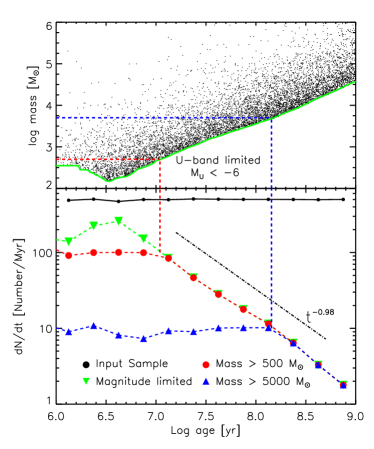
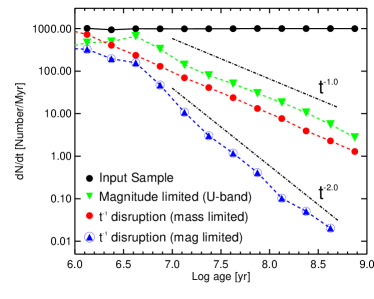
Figure 1: Left: Analysis of an artificial cluster population at the distance of M33. The population contains $5\times 10^{5}$ clusters, sampled from a power-law mass function with index $-2$, and assuming a constant cluster formation rate. The top panel shows the mass distribution for the observable part of the population – the detection limit is denoted by the solid line. This takes into account evolutionary fading, and the sample is assumed to be limited by the $U$-band, as is most commonly the case in extragalactic studies. The bottom panel shows the number of clusters per logarithmic age bin (${\textup{d}N/}\textup{d}\tau$): the dark solid line corresponds to all clusters ‘formed’ (i. e.  the entire simulated set), while the dashed green line tracks ‘observed’ clusters, i. e.  those above the detection limit. The theoretical expectation is for a magnitude limited sample to follow a simple power law distribution, whereas the introduction of a mass limit segments the distribution into a flat and a power law part (the transition is dictated by the mass cut and the point where incompleteness sets in). Right: A similar population, according to the predictions of MID. This presents the age distribution of a cluster population with a constant cluster formation rate and an imposed a $\tau^{-1}$ disruption law.

2.1 Age-mass diagram

This plot simply shows the number of clusters with increasing age. Log-bins accentuate the increase of the number of high mass clusters with increasing age. This arises because the sample grows with time – a ‘size-of-sample’ effect. As the sample increases, so does the likelihood of producing a massive cluster.

2.2 Detection limit

Unlike the top envelope of the age-mass diagram, the line along the bottom of the distribution is not caused by statistics, but the detection limit of our modelled observations. As clusters fade with time, this constant limiting flux translates into an increasing limiting mass.

In most of the cases observed cluster samples will be luminosity limited. As the population ages, clusters of higher mass fade below the detection limit. We have denoted this by a green line, representing the mass of a cluster with $M_{U}=-6$ (adapted to the study of M33 that will follow) at a given age. $U$ band is normally the limiting filter in observational studies and we emulate the detection limit in this plot.

2.3 Age distribution – the ${\textup{d}N/}\textup{d}\tau$ plot

The lower panel shows the main diagnostic used in the study of cluster disruption. The vertical axis gives the number of clusters our imaginary galaxy formed in each log-age bin, normalised to unit time (in this case one Myr). Here we present the input sample as a solid line: a constant CFH gives rise to a flat line. This will not, however, be observed, due to the detection limit.

2.4 A magnitude-limited sample

The green line shows all clusters that lie above the detection limit in each log-age bin and displays the characteristic power-law shape found in all observational studies. The interpretation of this plot is far from trivial: this $\tau^{-1}$ shape means that 90% of the population is lost with each age dex. MID interprets this as 90% of clusters dissolving each age dex ( in M33, [Sarajedini & Mancone(2007), Sarajedini & Mancone 2007]). In this example, however, this is due to detection incompleteness. Thus, a model has to treat fading and dissolution as two separate and concurrent causes of cluster disappearance.

2.5 Taking mass cuts

Having established the above, we can now perform a simple test for the mass dependence of cluster disruption: cutting the sample according to mass.

In the ${\textup{d}N/}\textup{d}\tau$ plot we present two mass cuts as a red and blue line respectively. Both cuts split the power-law distribution to a composite shape: a flat part, i.e. a constant cluster formation rate, and a power-law decline, due to clusters fading below the detection limit.

3 Observational study

After understanding the caveats inherent in the study of the ${\textup{d}N/}\textup{d}\tau$ plot, we can proceed to plot the distribution of an observed cluster sample.

We obtained the age and mass of a sample of $\sim 350$ bona fide clusters in M33 (spanning the entire surface of the galaxy, an unbiased, HST-selected sample; [Sarajedini & Mancone(2007), San Roman et al.(2009), Sarajedini & Mancone 2007, San Roman et al. 2009]) using UBVI imaging from the Local Group Survey ([Massey et al.(2006), Massey et al. 2006]). The SFR is known to have been constant for $\sim 1$ Gyr in M33, making it ideal for our study. Fig. 2 presents the age distribution of the magnitude-limited sample (left) and a mass cut (right). It exhibits the same shape as the ${\textup{d}N/}\textup{d}\tau$ plot of Fig. 1 (left), with a flat part leading to a power-law.

We also provide a direct test of MID in Fig. 1 (right panel), where we create a population that destroys 90% of its clusters each age dex and is subject to evolutionary fading.

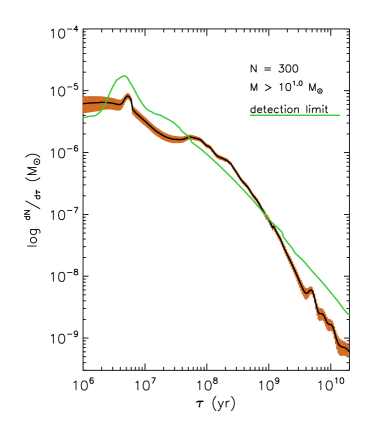
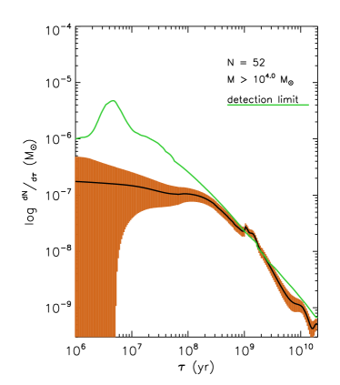
Figure 2: Left panel: A ‘smoothed’ ${\textup{d}N/}\textup{d}\tau$ plot: here we represent each measurement as a Gaussian, where the peak occurs at the best fit value (from 3DEF) and the wings are shaped after the uncertainty in the age fit (defined as the extrema calculated by 3DEF). This minimises the effect of uncertain measurements on the shape of the distribution, as an erratic measurement will be represented by a flat Gaussian. The solid green line is a prediction of the ${\textup{d}N/}\textup{d}\tau$ of a luminosity limited sample. It is the detection limit of Fig. 1 (left), inverted to reflect the maximum expected number of detections, given the detection limit (due to the complex scaling of the ${\textup{d}N/}\textup{d}\tau$ plot we have normalised the two lines at 1 Gyr). Right panel: the same plot with an imposed mass cut at $10^{4}$ M_⊙. The obvious flattening with respect to the magnitude limited sample on the left strongly supports a mass dependence in the cluster disruption process (consistent with BL03).

3.1 Observed ${\textup{d}N/}\textup{d}\tau$ plot

In order to dampen the effect of local overdensities in the ${\textup{d}N/}\textup{d}\tau$ plot (caused by uncertainties in the SSP models), in Fig. 2 we represent each age by a Gaussian, where the wings are defined by the uncertainty. The result is consistent with a $\tau^{-1}$ power-law for a magnitude-limited sample.

Crucially, as predicted by the models of Fig. 1 (left), taking a mass cut produces a composite structure, with a flat initial part and a power-law decline at older ages.

This demonstrates that an observed sample needs to be interpreted as the result of fading and dissolution at different timescales.

3.2 Mass independent dissolution plus fading

We have argued so far that the observed ${\textup{d}N/}\textup{d}\tau$ plot will show a combination of disruption and fading. The right hand side panel of Fig. 1 shows the combined effect of 90% dissolution (the MID hypothesis) and 90% disappearance due to fading. This results in a very steep power law decline (blue line) that is inconsistent with the observations of Fig. 2.

This result stands firmly against the MID cluster disruption model and implies the existence of a mass dependence.

4 Summary

Sample incompleteness causes a $\tau^{-1}$ decline in the observed age distribution of cluster populations. Size-of-sample effects and thorough statistical methods can help to interpret the disruption process at play. The fundamental difference between magnitude- and mass-limited samples can then be used to discover the underlying physics. Our results from the nearby population of M33 are inconsistent with mass-independent disruption of a fixed fraction of clusters per age dex.

References

- [Baumgardt & Makino(2003)] Baumgardt, H., & Makino, J. 2003, MNRAS, 340, 227
- [Boutloukos & Lamers(2003)] Boutloukos, S. G., & Lamers, H. J. G. L. M. 2003, MNRAS, 338, 717
- [Fall et al.(2005)] Fall, S. M., Chandar, R., & Whitmore, B. C. 2005, ApJL, 631, L133
- [Larsen(2009)] Larsen, S. S. 2009, A&A, 503, 467
- [Gieles(2009)] Gieles, M. 2009, MNRAS, 394, 2113
- [Sarajedini & Mancone(2007)] Sarajedini, A., & Mancone, C. L. 2007, AJ, 134, 447
- [San Roman et al.(2009)] San Roman, I., Sarajedini, A., Garnett, D. R., & Holtzman, J. A. 2009, ApJ, 699, 839
- [Massey et al.(2006)] Massey, P., Olsen, K. A. G., Hodge, P. W., Strong, S. B., Jacoby, G. H., Schlingman, W., & Smith, R. C. 2006, AJ, 131, 2478
- [Spitzer(1958)] Spitzer, L. J. 1958, ApJ, 127, 17