Neptune Trojans and Plutinos: colors, sizes, dynamics, and their possible collisions

Neptune Trojans and Plutinos are two sub-populations of Trans-Neptunian Objects located in the 1:1 and the 3:2 mean motion resonances with Neptune, respectively, and therefore protected form close encounters with the planet. However, the orbits of these two kinds of objects may cross very often, allowing a higher collisional rate between them than with other kinds of Trans-Neptunian Objects and a consequent and size distribution alteration of the two sub-populations.

Observational colors and absolute magnitudes of Neptune Trojans and Plutinos show that: i) there are no intrinsically bright (large) Plutinos at small inclinations; ii) there is an apparent excess of blue and intrinsically faint (small) Plutinos; and iii) Neptune Trojans possess the same blue colors as Plutinos within the same (estimated) size range do.

For the present sub-populations we analyze the most favorable conditions for close encounters / collisions to occur and address if there could be a link between those encounters and the sizes and/or colors of Plutinos and Neptune Trojans. We also perform a simultaneous numerical simulation of the outer Solar System over 1 Gyr for all these bodies in order to estimate their collisional rate.

We conclude that orbital overlap between Neptune Trojans and Plutinos is favored for Plutinos with high libration amplitudes, high eccentricities and low inclinations. Additionally, with the assumption that the collisions can be disruptive creating smaller objects not necessarily with similar colors, the present high concentration of small Plutinos at low inclinations can thus be a consequence of a collisional interaction with Neptune Trojans and such hypothesis should be further analyzed.

1 Introduction

Trans-Neptunian Objects (TNOs), also known as Kuiper Belt Objects (KBOs), are a population of small and primitive icy bodies orbiting (mostly) beyond Neptune. Their study is one of the most significant ways to obtain information on the early ages of the Solar System.

Based on some distinct dynamical properties, the TNOs can be subdivided in several different sub-populations, often also called families or groups. Subdivide them as a function of their physical properties seems to be far more complex. TNOs have surface colors so diverse that can go from blue/neutral (i.e. solar-like) to extremely red. A possible explanation for the wide variety of colors was originally proposed by Luu & Jewitt (1996) with the collisional resurfacing model. In this model, the competition between surface reddening, due to cosmic-ray bombardment, and a resurfacing with frozen material (assumed to be bluer) withdrawn from beneath its crust by impact collisions could be responsible for the observed wide range of surface colors. As the model seems to fail, at least in its simple form, more complex forms have been proposed. Namely, collisional resurfacing combined with cometary activity (Delsanti et al., 2004), and collisional resurfacing with layered reddening and even re-bluing by cosmic-rays (Gil-Hutton, 2002). An alternate idea proposes that surface colors are primordial (Tegler et al., 2003b, and references therein). More recently, Grundy (2009) shows that an object could lose its redness simply by ice sublimation (without resurfacing). Such could explain the lack of red colors among TNOs that evolved into Jupiter family comets due to their closeness to the Sun. Yet, as the aforementioned work acknowledges, the existence of the blue/neutral TNOs at heliocentric distances where ices do not sublimate suggests the existence of other coloring mechanisms. Our understanding on the origin and eventual alteration of TNOs colors is still very limited and, up to the present, none of these approaches lead to a fully consistent explanation for the color diversity (for a review see Doressoundiram et al., 2008).

Among the TNOs, two sub-populations caught our attention: the Neptune Trojans and the Plutinos. Neptune Trojans are the small bodies trapped in a 1:1 mean motion orbital resonance with Neptune, also with orbital eccentricities lower than 0.1. Roughly they co-orbit with Neptune concentrated $60^{\circ}$ ahead and $60^{\circ}$ behind Neptune’s position. Chiang & Lithwick (2005) proposed that Neptune Trojans formed by in-situ accretion from small-sized debris once Neptune’s migration has stopped. On the other hand, other works indicate they can survive planetary migration (Nesvorný & Dones, 2002; Kortenkamp et al., 2004) and, more recently, due to the discovery of a large population of high inclination Neptune Trojans, Nesvorný & Vokrouhlický (2009) sustain they were captured during planetary migration Compared to TNOs Neptune Trojans seem to be quite small in size (diameters $D<100$ km) and also slightly blue.

At the time of our analysis 6 Neptune Trojans were known, all of them librating around the Lagrangian point $L_{4}$.

Plutinos are those trapped in a 3:2 mean motion orbital resonance with Neptune, with eccentricity values ranging between 0.1 and 0.3. Unlike Trojans, the colors of Plutinos vary from blue/neutral to the very red, and their sizes range from a few tens of km to a few thousands (note that Pluto is a Plutino). Roughly, Plutinos possess semi-major axes within $39<a<40.5$ AU. Through long-term dynamical evolution studies Lykawka & Mukai (2007) identified 98 Plutinos and that will be our reference.

Being locked at the 3:2 resonance, Plutinos can periodically cross the orbit of Neptune without colliding with it. However, this protection from collisions is not possible for Neptune Trojans and Plutinos. A first look at the geometry of these two populations suggests that they might even collide frequently.

The analysis of the collisional resurfacing model by Thébault & Doressoundiram (2003) and Thébault (2003) found that Plutinos were significantly more affected by collisions than other TNOs. Since, observationally, Plutinos did not exhibit bluer colors than all other TNOs taken as a whole, the aforementioned work strongly argued against the collisional resurfacing model, at least as major cause for the color diversity of TNOs. Neptune Trojans were not included in Thébault & Doressoundiram’s simulations, though, since they were not known at the time. Notwithstanding the arguments against it, the collisional resurfacing that was analyzed was a very simple model. For instance, the possibility of collisional disruption of differentiated bodies producing fragments or ruble-piles with surface colors distinct from those of the parent bodies has not been taken into account in the collisional resurfacing models yet. Naturally, the possible outcomes of this scenario would be far more complex and our understanding of the physics of collisional processes between the icy TNOs is still limited (see review by Leinhardt et al., 2008). Nonetheless, both a collisional family of TNOs associated with (136108) Haumea and a collisional system of satellites associated with Pluto have been detected (Brown et al., 2007; Stern et al., 2006; Canup, 2005).

Surveys show a power-law for the size distribution of TNOs with slope change at $D\sim 100$ km (Bernstein et al., 2004), which is most consistent with TNOs being gravity dominated bodies with negligible material strength. Objects larger than $\sim 100$ km are difficult to disrupt, hence likely primordial, and objects smaller than this are expected to be shattered due to disruptive collisional evolution (Kenyon et al., 2008; Pan & Sari, 2005).

de Elía et al. (2008) studied the collisional evolution of Plutinos considering only Plutino-Plutino collisions. They infer that any eventual slope change at $D\sim 40-80$ km on the power-law size distribution of Plutinos should be primordial and not of collisional origin. Yet, they find that collisional populations may form from the breakup of objects larger than $100$ km, and if those populations form at low inclinations their fragments will likely stay in the resonance.

On Sect. 2 we will analyze the observational data relative to Neptune Trojans and Plutinos. We will discuss two particular observational properties: 1) there is an apparent “excess” of small blue Plutinos and these happen to be also in the same size range and to possess the same colors as the known Neptune Trojans, and 2) there is a concentration of small Plutinos, and absence of large ones, at low orbital inclinations. The eventual collisional interaction between Plutinos and Neptune Trojans has not been analyzed in previous works. Since their geometry points to the existence of mutual collisions, the existence of an eventual link between the colors and sizes of Neptune Trojans and Plutinos and their interactions/collisions motivated us to this work. On Sect. 3 we will study the dynamics of Neptune Trojans and Plutinos, separately, focusing on their orbits around the Lagrangian point $L_{4}$. On Sect. 4 we will discuss the possibility of collisions between Neptune Trojans and Plutinos and the best conditions for this to happen. Finally, on Sect. 5 we will present our conclusions.

2 Observational Results and Discussion

In Table LABEL:tab:tab_1 we summarize the orbital elements, $B-R$ colors, and R-filter absolute magnitudes ($H_{R}$) for 4 Neptune Trojans (from Sheppard & Trujillo, 2006) and 41 Plutinos (see references on the table). In Fig. 1 we plot the orbital inclination vs orbital eccentricity of all these objects, together with their $B-R$ colors, indexed on a color palette on the right hand side of the figure, and in which objects are plotted proportionally to their estimated diameter also indexed on the top of the figure.

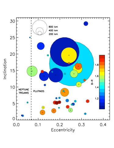
Figure 1: Orbital inclination vs eccentricity, estimated size, and color of Neptune Trojans and Plutinos for which those properties have been measured.

The diameters of these objects (in kilometers) are estimated from the absolute magnitudes using the formula (Russell, 1916):

$$D_{(km)}=2\times\sqrt{\frac{2.24\times 10^{16}\times 10^{0.4(-27.10-H_{R})}}{p_{R}}}\,,$$ (1)

where $H_{R}$ is the R-filter absolute magnitude, and the R-filter albedo is taken as $p_{R}=0.09$ (Brown & Trujillo, 2004). A size estimation exception is made for Pluto which is represented with $D=2390$ km. A vertical dashed line separates Neptune Trojans, located on the left side of the figure, from Plutinos, located on the right side.

A first look at Fig. 1 shows that:

(i)

all Trojans are blue, small ($D<100$ km) compared to the size distribution of Plutinos, and possess small eccentricities;

(ii)

there is an apparent concentration of small Plutinos at low inclination values and a concentration of large Plutinos at high inclinations;

(iii)

Plutinos have larger eccentricity values than Trojans, and their colors range from blue to red appearing randomly distributed in inclination and eccentricity.

(iv)

all Plutinos within the same (estimated) size range as Neptune Trojans possess blue colors.

It is important to note that the small sized Plutinos, which are also as blue as Neptune Trojans, are randomly scattered in eccentricity and inclination whereas the low inclined Plutinos are all relatively small but range from blue to red colors.

Based on these properties we decide to explore two possible scenarios:

(1)

could the equally blue colors of the equally sized Plutinos and Neptune Trojans be the result of some collisional interaction between both populations?

(2)

could the concentration of small Plutinos at low inclinations be the result of some collisional interaction between them and Neptune Trojans?

Why these two scenarios? From the simulations by Thébault & Doressoundiram (2003) and Thébault (2003), which analyzed the collision rates among all TNOs simultaneously (except for Neptune Trojans that were not known at the time), Plutinos received more collisions than any other sub-population. The number/energy of those collisions also seemed independent of their orbital parameters. That is, Plutinos seemed under the same collisional environment regardless of their high or low inclination and/or eccentricity values.

Therefore, since the possible effects of a significant number of Neptune Trojans were not considered in the aforementioned simulations in this work we explore if and how these Trojans could be the major cause of the non-homogeneity of surface properties observed among Plutinos and the (apparent) homogeneity of surface properties observed for Neptune Trojans.

Let us grasp scenario (1). The members of the collisional families associated with (136108) Haumea possess very similar bluish colors (Brown et al., 2007). It is reasonable to hypothesize that if Neptune Trojans collided heavily with part of the Plutino population the collision outcomes could be similar in color. Considering that assumption, for this scenario to be possible we need to find a similar collision rate between Trojans and Plutinos independent of the eccentricity and/or inclination values of Plutinos since the small ($D<100$ km) and blue Plutinos are homogeneously scattered both in eccentricity and inclination.

As to scenario (2), we are considering a less strict hypothesis in which the collision outcomes of collisions between Neptune Trojans and part of the Plutino population are not necessarily equal in color. The Pluto system has, presumably, a collisional origin, however, while Charon, Nix, and Hydra possess similar colors Pluto is quite distinct (e.g. Stern, 2009). Let us assume that the disruption of large layered TNOs could generate several objects with distinct colors either from fragments coming from different layers with different colors or from reaccretion of different parts of a heterogenous cloud of debris. Hence, collisions would generate both blue and red, small and medium objects ($D<300$ km). For this scenario to be possible we need to find a much higher collision rate between Trojans and the Plutinos with low inclination values than with the Plutinos at high inclinations. Also, given that we do not see neither red nor mid/large-sized Neptune Trojans, whereas we see it among Plutinos in the presumable region of collisions, the primordial size and color distributions of Trojans and Plutinos should not have been similar.

Note that even though resonant objects are known to possess large variations of their eccentricity and/or inclination values, Nesvorný & Roig (2000) showed the existence of two dynamical populations of Plutinos, separating at $i\sim 10^{\circ}$, which do not seem to easily mix. Consequently, any different collisional/surface evolution that both populations might have had in the past should still be detectable today.

In order to test if the low inclined Plutinos are indeed smaller than the other ones we use the Kolmogorov-Smirnov test (Press et al., 1992; Kolmogorov, 1933; Smirnov, 1939). We successively compare the absolute magnitude $H_{R}$ distribution of our 41 Plutinos (with measured $B-R$ colors) having $i<i_{c}$ with those having $i\geq i_{c}$, varying $i_{c}$ from $4^{\circ}$ to $15^{\circ}$ in increments of $0.5^{\circ}$. Two significant solutions exist: a) Plutinos with $i<8^{\circ}$ are intrinsically fainter, and assumed to be smaller, than those above $8^{\circ}$ with a (one-tailed) significance $p=0.0024$; b) Plutinos with $i<13^{\circ}$ are intrinsically fainter than those above $13^{\circ}$ with a significance $p=0.0030$. Even though we do not obtain an unique solution for the best inclination value that separates the larger (brighter) from the smaller (fainter) Plutinos, we can conclude that the low-inclined ones are in fact smaller. Figure 2 shows the cumulative distribution functions of absolute magnitudes for the higher inclined and lower inclined Plutinos in both solutions.

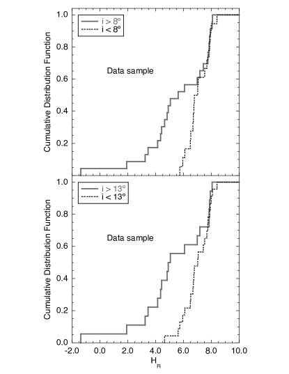
Figure 2: Cumulative distribution function of absolute magnitudes $H_{R}$ for Plutinos above and below $8^{\circ}$ of inclination (top) and Plutinos above and below $13^{\circ}$ (bottom). The incompatibility of distributions between the higher and lower inclined Plutinos is similar in both cases. There is an evident lack of intrinsically bright (large) objects among the lower inclined Plutinos.

We will proceed with the study of the dynamics of Plutinos and Neptune Trojans and investigate their possible collisions.

3 Dynamical Evolution

In previous section we discussed the possible relations between the colors of Plutinos and Neptune Trojans, and the eventual collisions between them. It is now our goal to test the possibility of collisions numerically. For that purpose we will simulate the outer Solar System evolution, where the TNOs are considered massless. This hypothesis is essential to speed up the integrations. The equation of motion for planets is given by

$$\ddot{\textbf{r}}_{i}+\mathcal{G}(m_{s}+m_{i})\frac{\textbf{r}_{i}}{r_{i}^{3}}=\sum_{j\neq i}^{N_{P}}\mathcal{G}m_{j}\Bigg{(}\frac{\textbf{r}_{j}-\textbf{r}_{i}}{\left|\textbf{r}_{j}-\textbf{r}_{i}\right|^{3}}-\frac{\textbf{r}_{j}}{r_{j}^{3}}\Bigg{)}\,,$$ (2)

where $\textbf{r}_{i}$ is the vector position of the planet, $\mathcal{G}$ the gravitational constant, $m_{s}$ the mass of the Sun, $m_{i}$ the mass of the planet, and $N_{P}$ is the total number of planets. In our simulations we will only take into account the four giant planets. The effect of the inner Solar System in the dynamics of the Kuiper belt objects is only residual and by neglecting it we may use a larger step-size for numerical simulations and considerably decrease the length of the simulations.

For TNOs, since they are assumed massless, the equation of motion is given by

$$\ddot{\textbf{r}}_{k}+\mathcal{G}m_{s}\frac{\textbf{r}_{k}}{r_{k}^{3}}=\sum_{j}^{N_{P}}\mathcal{G}m_{j}\Bigg{(}\frac{\textbf{r}_{j}-\textbf{r}_{k}}{\left|\textbf{r}_{j}-\textbf{r}_{k}\right|^{3}}-\frac{\textbf{r}_{j}}{r_{j}^{3}}\Bigg{)}\,,$$ (3)

where $\textbf{r}_{k}$ is the vector position of the TNO. By adopting the above equations we assumed that planets and TNOs are only perturbed by the remaining planets, i.e., the TNOs are considered as test particles. The only exception will be the Pluto-Charon system barycenter, which will be considered as a planet because of its important mass. Indeed, some Plutinos may be pushed out of the 3:2 resonance by Pluto into close encounters with Neptune (Yu & Tremaine, 1999; Nesvorný et al., 2000).

In our simulations we will use the symplectic integrator from Laskar & Robutel (2001), with an integration step-size of 0.1 yr. The system is composed of 5 planets (Table 4), 6 Trojans (Table 5) and 98 Plutinos (Table LABEL:tab:tab_4).

3.1 Resonant Motion

Since both Trojans and Plutinos are resonant objects we will briefly recall here the bases of resonant motion, following Murray & Dermott (1999). Consider then a TNO in some resonance with Neptune. We assume for simplicity, that Neptune is in a circular orbit and that all motion takes place in the plane of its orbit. We also ignore any perturbations between the two bodies as we are only interested in how resonant relationships lead to repeated encounters.

We can examine the geometry of resonance for a general case by first considering two bodies moving around the Sun, in circular and coplanar orbits. So, let us assume that

$$\frac{n^{\prime}}{n}=\frac{p}{p+q}\,,$$ (4)

where n and n’ are the mean motions of Neptune and the TNO, respectively (for Trojans $p=1$ and $q=0$, while for Plutinos $p=2$ and $q=1$). If the two bodies are in conjunction at time $t=0$, the next conjunction will occur when $(n-n^{\prime})t=2\pi$, and the period, $T_{con}$, between successive conjunctions is given by

$$T_{con}=\frac{2\pi}{n-n^{\prime}}=\frac{p}{q}T^{\prime}=\frac{p+q}{q}T\,,$$ (5)

where T and T’ are the orbital periods of the two bodies.

Now consider the case when $e=0$, $e^{\prime}\neq 0$, and $\dot{\varpi}^{\prime}\neq 0$, where e denotes the eccentricity for Neptune and e’ and $\varpi^{\prime}$ denotes the eccentricity and longitude of pericentre of the TNO respectively. If the resonant relation

$$(p+q)n^{\prime}-pn-q\dot{\varpi}^{\prime}=0$$ (6)

is satisfied, then we can rewrite Eq.(4) as

$$\frac{n^{\prime}-\dot{\varpi}^{\prime}}{n-\dot{\varpi}^{\prime}}=\frac{p}{p+q}\,,$$ (7)

where $n^{\prime}-\dot{\varpi}^{\prime}$ and $n-\dot{\varpi}^{\prime}$ are relative motions. These can be considered as the mean motions in a reference frame, co-rotating with the pericentre of the TNO. From the point of view of this reference frame, the orbit of the TNO is fixed or stationary. If the resonant relation given in Eq.(6) holds, the corresponding resonant argument is

$$\varphi=(p+q)\lambda^{\prime}-p\lambda-q\varpi^{\prime}\,,$$ (8)

where $\lambda$ and $\lambda^{\prime}$ denote the mean longitude of Neptune and the TNO, respectively. At a conjunction of the two bodies, $\lambda=\lambda^{\prime}$ and we have

$$\varphi=q(\lambda^{\prime}-\varpi^{\prime})=q(\lambda-\varpi^{\prime})\,.$$ (9)

Thus, $\varphi$ is a measure of the displacement of the longitude of conjunction from pericentre of the TNO. By computing the derivative of the resonant angle $\varphi$, we get

$$\dot{\varphi}=(p+q)n^{\prime}-pn-q\dot{\varpi}^{\prime}\,,$$ (10)

and $\dot{\varphi}=0$ from Eq.(6). In a more general situation, we will have $\dot{\varphi}\neq 0$, but in order to preserve the resonant equilibrium $\varphi$ will librate around an equilibrium position $\varphi_{0}$, obtained when $\dot{\varphi}=0$. The libration amplitude $\Delta\varphi$ will depend on the initial conditions and perturbations from the other bodies in the system and may reach large values. As a consequence, it is possible that the orbits of two distinct bodies librating around different equilibrium positions intercept at some point.

Along with the orbital parameters of the Trojans and Plutinos that we used in our simulations, in Table 5 and Table LABEL:tab:tab_4, respectively, we provide the equilibrium libration angle, the main libration period and amplitude of each TNO obtained over the next 250 Kyr.

3.2 Trojans

Neptune Trojans are resonant objects in a 1:1 mean motion resonance with Neptune. In our model we computed the motion of the six Neptune Trojans listed in Table 5. In Fig. (3), we show the behavior of all known Trojans, along time, in a co-rotating frame with Neptune for 100 Myr. Each dot shows the position of the TNO every 10 kyr.

As expected, we see in Fig.3 that all Trojans orbit around the Lagrangian point $L_{4}$, and execute tadpole-type orbits. This kind of orbits represents stable oscillations in the vicinity of the Lagrangian equilibrium point (e.g. Giuliatti Winter et al., 2007). The differences between the shape of their orbits, depend on the libration amplitude, but also on their orbital eccentricity and inclination values. Trojan 2007VL305, that execute the most scattered orbit, also presents the largest eccentricity and inclination ($e=0.062$ and $i=28^{\circ}$). On the other hand, for small values of these two orbital parameters, the TNOs remain roughly in the path of Neptune’s orbit, only changing its relative position to the planet due to libration.

$\begin{array}[]{cc}\includegraphics[scale={0.25},angle={0}]{Figures/2001QR322.ps}&\includegraphics[scale={0.25},angle={0}]{Figures/2004UP10.ps}\\ \includegraphics[scale={0.25},angle={0}]{Figures/2005TN53.ps}&\includegraphics[scale={0.25},angle={0}]{Figures/2005TO74.ps}\\ \includegraphics[scale={0.25},angle={0}]{Figures/2006RJ103.ps}&\includegraphics[scale={0.25},angle={0}]{Figures/2007VL305.ps}\end{array}$

Figure 3: Orbital evolution of the Neptune Trojans (in green) listed in Table 5 over 100 Myr in the co-rotating frame of Neptune (in blue). Each panel shows the projection of the TNO position every 10 Kyr in the orbital plane of Neptune. $x$ and $y$ are spatial coordinates centered in the star and rotating with Neptune, normalized by the Neptune-Sun distance. All Trojans orbit around the Lagrangian point $L_{4}$, and execute tadpole-type orbits. More scattered orbits correspond to higher values of the eccentricity and inclination, while distance to the $L_{4}$ point depend on the libration amplitude.

In Table 5 we provide the libration amplitude and period for all Trojans. While amplitudes can vary from only $6^{\circ}$ to $26^{\circ}$, the periods of libration remain around 9 Kyr for all objects. Trojan 2001QR322 presents the largest libration amplitude and therefore moves further away of the equilibrium point $L_{4}$. As a consequence, its orbit will be more susceptible of being destabilized by gravitational perturbations from the planets and other bodies in the system. Indeed, in our long-term numerical simulations (Sect. 4.1) this TNO will abandon the Trojan orbit after 112 Myr and become a Kuiper belt object.

3.3 Plutinos

Plutinos are resonant TNOs in a 3:2 mean motion resonance with Neptune. Thus, like Trojans, although they can cross the orbit of Neptune, they are protected from possible encounters with this planet. In Fig.4 we have drawn the typical path of a Plutino in the co-rotating frame of Neptune, for three different values of the eccentricity ($e=0.1$, 0.2 and 0.3).

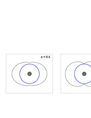
Figure 4: Typical path of a Plutino (dotted line) in the rotating frame of Neptune (full line) for different eccentricity values ($e=0.1$, 0.2 and 0.3). The position of the Plutino was drawn for equal time intervals. Only high eccentricity values ($e>0.2$) allow the Plutino to cross the orbit of Neptune. Due to the 3:2 mean motion resonance the trajectories are repeated every two orbits of the TNO around the Sun.

These plots are drawn assuming that the Plutino is at exact resonance ($\dot{\varphi}=0$), which is not true, because the orbit is librating around an equilibrium position $\varphi_{0}$ (Eq.8). As a consequence, in a more realistic situation we will observe an oscillation of those paths as the one represented in Fig.5. In Table LABEL:tab:tab_4 we provide the libration amplitude and period for all Plutinos. The equilibrium libration angle for them all is $\varphi_{0}=\pm 180^{\circ}$, but the amplitudes of libration can be as small as $7^{\circ}$ for Plutino 1996TQ66 or as wide as $120^{\circ}$ for Plutinos 1995QY9 and 2001KN77. The libration periods, $P_{lib}$, vary between 14.5 and 26.6 Kyr, the average being around 20 Kyr. For comparison, the values for Pluto are $\Delta\varphi=79.7^{\circ}$ and $P_{lib}=19.9$ Kyr.

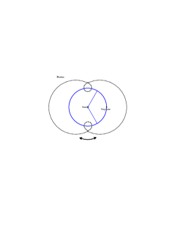
Figure 5: Libration motion of the orbit of a Plutino.

In our model we computed the motion of about 100 Plutinos, whose orbital parameters are listed in Table LABEL:tab:tab_4. All objects present moderate eccentricities and inclinations, ($\bar{e}\sim 0.23$ and $\bar{i}\sim 10.4^{\circ}$). According to Malhotra (1995) these values can be a consequence of the resonant mechanism of capture, during the residual planetesimal cleaning in the vicinity of the young giant planets. Due to Neptune’s migration, the eccentricity and inclination of the Plutinos are pumped after capture in resonance.

In Fig.6 we show the behavior of six Plutinos, along time, in a co-rotating frame with Neptune for 100 Myr, each dot showing the position of the object every 10 Kyr. Because Plutinos are much more numerous than Trojans, we can only represent a small fraction of them. We have chosen the most representative cases, namely, the Plutino with the smallest and widest libration (1996TP66 and 2001KN77, respectively), the Plutinos with smallest and highest eccentricity (2003VS2 and 2005GE187, respectively), and the Plutinos with smallest and highest inclination (2002VX130 and 2005TV189, respectively).

$\begin{array}[]{cc}\includegraphics[scale={0.25},angle={0}]{Figures/1996TP66.ps}&\includegraphics[scale={0.25},angle={0}]{Figures/2001KN77.ps}\\ \includegraphics[scale={0.25},angle={0}]{Figures/2003VS2.ps}&\includegraphics[scale={0.25},angle={0}]{Figures/2005GE187.ps}\\ \includegraphics[scale={0.25},angle={0}]{Figures/2002VX130.ps}&\includegraphics[scale={0.25},angle={0}]{Figures/2005TV189.ps}\end{array}$

Figure 6: Orbital evolution of some Plutinos (in red) taken from Table LABEL:tab:tab_4 over 100 Myr in the co-rotating frame of Neptune (in blue). Each panel shows the projection of the TNO position every 10 Kyr in the orbital plane of Neptune. $x$ and $y$ are spatial coordinates centered on the star and rotating with Neptune, normalized by the Neptune-Sun distance. We have chosen the most representative cases, namely, Plutino 1996TP66, with the smallest libration amplitude ($\Delta\varphi=7.2^{\circ}$, $e=0.328$, $i=5.6^{\circ}$), Plutino 2001KN77, with the widest libration amplitude ($\Delta\varphi=120.4^{\circ}$, $e=0.242$, $i=2.4^{\circ}$), Plutino 2003VS2, with the smallest eccentricity ($e=0.072$, $i=14.8^{\circ}$), Plutino 2005GE187, with the highest eccentricity ($e=0.329$, $i=18.2^{\circ}$), Plutino 2002VX130, with the smallest inclination ($e=0.220$, $i=1.3^{\circ}$), and Plutino 2005TV189, with the highest inclination ($e=0.186$, $i=34.5^{\circ}$).

As expected, depending on the eccentricity values, the orbits of the Plutinos are all in good agreement with the paths shown in Fig.4. Because of the libration motion of the orbits (Fig.5) their trajectories approach or cross the Lagrangian points $L_{4}$ and $L_{5}$, that is, the Plutinos orbits share the same spatial zone as the Neptune Trojans.

4 Numerical Simulations

In Sect.2 we have shown that, although Neptune Trojans and Plutinos appear to have different origins, some of their properties indicate that the two types are quite identical, suggesting that there must be some sort of communication between them. Indeed, in the previous section we saw that due to the libration motion of the orbits there is a wide zone of spatial overlap around the Lagrangian point $L_{4}$ of Neptune. As a consequence, we may expect close encounters and collisions between the two kinds of TNOs to occur at a higher rate than in the remaining Kuiper belt, resulting in a change of the size distributions of the two populations.

In order to test this possibility we simulated the long-term future evolution of the outer Solar System for 1 Gyr. The orbits of the outer planets, the Neptune Trojans and the Plutinos are integrated simultaneously according to the model described in the beginning of Sect.3.

4.1 Stability of the Neptune Trojans

The stability of the Neptune Trojans orbits is an important issue on the dynamics of the outer Solar System. According to Dvorak et al. (2007) Trojans with low-inclined orbits are less stable. The stability area around $L_{4}$ and $L_{5}$ disappears after about $10^{8}$ yr for low inclinations, while this stability zone is still present for about $10^{9}$ yr for large inclinations. More precisely, it was concluded that there exists a region ($20^{\circ}<i<50^{\circ}$) of higher stability for the Neptune Trojans, although only two have presently been found in this region (Table 5).

During our numerical simulations all Trojans remained stable within the limits shown in Fig.3 during 1 Gyr, except Trojan 2001QR322, which escapes from the Lagrangian $L_{4}$ point after about 112 Myr. This last observation was somehow unexpected, since Chiang et al. (2003) concluded that this same Neptune Trojan was stable over 1 Gyr. This difference of behaviors is a consequence of a modification in the initial conditions (Table 5), obtained with new observational data. This event is more or less in agreement with the results from Dvorak et al. (2007), because Trojan 2001QR322 is the one with smallest inclination ($i=1.3^{\circ}$). Although other Trojans with identical inclination values remained stable, we notice that Trojan 2001QR322 also has the widest libration amplitude ($\Delta\phi=26^{\circ}$) and its orbit is therefore more susceptible of being disturbed by planetary perturbations. This suggests that the stability of the Trojans is smaller for low-inclined orbits, but also for large libration amplitudes.

In Fig.7 we plot the long-term evolution of the orbital period and the eccentricity of the Trojan 2001QR322. The behavior of this object is extremely regular, until it undergoes a sudden increment of the eccentricity, which removes it form the 1:1 mean motion resonance with Neptune. Interestingly, just after escaping the resonance, the semi-major axis of this TNO is temporarily stabilized near the 3:2 resonance with Neptune, i.e., its orbit becomes very close to the Plutino’s orbits. However, contrary to regular Plutinos, the eccentricity undergoes important chaotic variations from nearly zero up to 0.3. This regime lasts for about 300 Myr, time after which the eccentricity grows to almost 0.8. As a consequence, close encounters with the planets become possible and the TNO leaves the area near to the 3:2 mean motion resonance. Later on, the same TNO seems to be captured in a 9/2 mean motion resonance with Neptune, and stays there for about 100 Myr. Finally, the orbit is again destabilized and the eccentricity grows to extreme values, and the TNO turns into a comet.

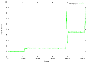
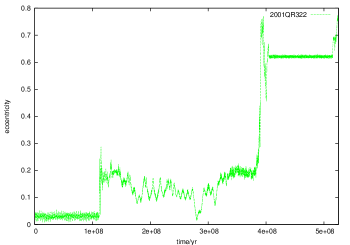
Figure 7: Long-term evolution of the orbital period (over Neptune’s orbital period) and the eccentricity of Trojan 2001QR322 for 525 Myr. Initially a Trojan, the orbit of this TNO is not stable and quits the 1:1 mean motion resonance after about 112 Myr. Then it jumps to different configurations until it becomes a comet and eventually collides with a planet or the Sun. In this simulation it is ejected from the Solar System after 525 Myr.

4.2 Stability of the Plutinos

The orbits of the Plutinos are believed to be stable as long as the libration amplitudes are smaller than $120^{\circ}$ (Nesvorný & Roig, 2000). For larger libration widths, the planetary perturbations will remove the TNO from its orbit in short time intervals. The same phenomena was observed for Trojans.

During our numerical simulations over 1 Gyr, 10 Plutinos over 98 quit their orbits (about 10%). In Table 1 we list all these bodies, as well as their libration width (Table LABEL:tab:tab_4). Contrary to expectations, we observe that only two Plutinos present libration amplitudes around $120^{\circ}$. The minimum libration width observed is around $40^{\circ}$. A possible explanation is that because Plutinos are not alone in their orbits and, according to Yu & Tremaine (1999) and Nesvorný et al. (2000), some Plutinos may be pushed out of the resonance by Pluto into close encounters with Neptune. Indeed, stability maps by Nesvorný & Roig (2000) only take into account the effect of the four giant planets.

Table 1: List of all unstable Plutinos during 1 Gyr.

Plutino	time (Myr)	$e$	$\Delta\varphi\,(^{\circ})$
2000FV53	69	0.168	117.76
2004FU148	230	0.235	94.67
2002GE32	500	0.232	73.14
1998WZ31	590	0.165	76.61
2004EW95	595	0.320	53.31
1995QY9	680	0.262	120.22
2003TH58	710	0.088	65.29
1993SB	720	0.317	53.19
2002XV93	820	0.127	42.70
2003UT292	840	0.292	80.69

In Fig.8 we plot the long-term evolution of the orbital period and the eccentricity of TNO 2000FV53. The initial 3:2 resonant configuration is abandoned just after 69 Myr, time after which the eccentricity increases progressively. The TNO then undergoes close encounters with the planets, which will increase the eccentricity even more, until it can reaches very high values. The Plutino 2000FV53 then becomes a short-period comet and eventually collides with a planet or the Sun. This mechanism has already been described as the responsible for the provision of short period comets into the inner Solar System (e.g. Morbidelli, 1997). In our simulation the aforementioned TNO is ejected from the Solar System after 150 Myr.

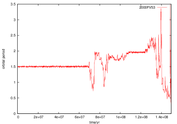
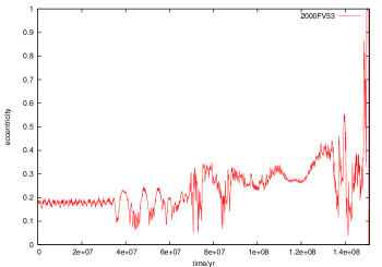
Figure 8: Long-term evolution of the orbital period (over Neptune’s orbital period) and the eccentricity for Plutino 2000FV53 for 150 Myr. Initially a Plutino, the orbit of this TNO is not stable and quits the 3:2 mean motion resonance just after about 69 Myr. Its eccentricity then increases progressively and the TNO becomes a short-period comet that eventually collides with a planet or the Sun. In this simulation it is ejected from the Solar System after 150 Myr.

4.3 Orbital overlap between Trojans and Plutinos

In Sect.3.3 we saw that because of libration, the Plutinos’ orbits can approach the Lagrangian point $L_{4}$. In order to check the extent of the orbital overlap between Neptune Trojans and Plutinos, in Fig.9 we plotted simultaneously their orbits in a co-rotating frame with Neptune. We used the Trojan 2007VL305 for all representations, since it has the most scattered orbit, maximizing the possibility of orbital merging with a Plutino. For the Plutinos we used the same bodies as in Sect.3.3, which correspond to the extreme cases of libration, eccentricity, and inclination. The only exception is that Plutino 1996TP66 (with the smallest libration width) has been replaced by Pluto, since a small libration amplitude does not allow the Plutino to flyby the Lagrangian points.

$\begin{array}[]{cc cc}\includegraphics[width=122.85876pt]{Figures/2007VL305_Pluto_a.ps}&\includegraphics[width=122.85876pt]{Figures/2007VL305_Pluto_b.ps}&\includegraphics[width=122.85876pt]{Figures/2007VL305_2001KN77_a.ps}&\includegraphics[width=122.85876pt]{Figures/2007VL305_2001KN77_b.ps}\\ \includegraphics[width=122.85876pt]{Figures/2007VL305_2003VS2_a.ps}&\includegraphics[width=122.85876pt]{Figures/2007VL305_2003VS2_b.ps}&\includegraphics[width=122.85876pt]{Figures/2007VL305_2005GE187_a.ps}&\includegraphics[width=122.85876pt]{Figures/2007VL305_2005GE187_b.ps}\\ \includegraphics[width=122.85876pt]{Figures/2007VL305_2002VX130_a.ps}&\includegraphics[width=122.85876pt]{Figures/2007VL305_2002VX130_b.ps}&\includegraphics[width=122.85876pt]{Figures/2007VL305_2005TV189_a.ps}&\includegraphics[width=122.85876pt]{Figures/2007VL305_2005TV189_b.ps}\end{array}$

Figure 9: Orbital evolution of the Trojan 2007VL305 (in green) and Pluto plus most of the Plutinos in Fig.6 (in red), over 1 Gyr in the co-rotating frame of Neptune (in blue). Left panel (a) shows the projection of the TNO position every 100 Kyr in the orbital plane of Neptune, while right panels (b) shows the projection of the TNO in the orbital plane of Neptune every 10 Kyr, only when the distance to this plane is smaller then $10^{-3}$ AU. We observe that orbital overlap is favored for Plutinos with high libration amplitudes, high eccentricity values and low inclined orbits.

Since the TNOs are not necessarily in the same orbital plane as Neptune (especially for those having large inclination values), two types of plots have been made: one where we plotted the projection of the TNO position in the orbital plane of Neptune (Fig.9a), and another where we plotted the projection of the TNO in the orbital plane of Neptune, only when the distance to this plane is smaller then $10^{-3}$ AU (Fig.9b), that is, less than 150 000 km, half of the Earth-Moon distance. Indeed, most of our Trojans have low inclinations and therefore lie close to Neptune’s orbital plane most of the time. As a consequence, near this plane close encounters with Plutinos are maximized.

The importance of plotting the two situations is clearly illustrated by the behavior of Pluto (Fig.9). At first glance, looking only to the projection on Neptune’s orbital plane, we observe a large zone shared by the orbits of the two kinds of TNOs, suggesting that close encounters may be a regular possibility. However, when we restrain the plot only to Neptune’s orbital plane, we observe that Pluto is never on this plane when it approaches $L_{4}$, preventing any close encounter with Trojans.

From the analysis of Fig.9, we can also conclude that Plutinos with large libration amplitudes (e.g. 2001KN77) maximize the chances of intercepting Trojans. This behavior was expected, as their orbits invade a large zone around the Lagrangian point $L_{4}$.

On the other hand, Plutinos with low eccentricity values ($e\sim 0.1$; e.g. 2003VS2), always avoid Trojans independently of its libration amplitude or orbital inclination, since the small eccentricity prevents them from crossing Neptune’s orbit. According to Fig.4, this result could also be expected, because for low eccentricity there is no interception of the Plutino and Neptune’s orbits.

Finally, when comparing the behavior of Plutinos in low-inclined orbits (2001KN77 and 2002VX130) with high-inclined ones (Pluto, 2003VS2, 2005GE187 and 2005TV189) we conclude that large orbital inclination decreases the chances of close encounters because the Plutino is never close to Neptune’s orbital plane when it crosses the orbit of the planet. The fact that Plutinos with low inclination share the Trojan space was expectable, as both TNOs remain close to the same orbital plane. However, Plutinos with high inclination could also approach the orbital plane of Neptune at the moment they are close to the Lagrangian points, which is not really observed.

From the above analysis (and also for the remaining 5 Trojans and 92 Plutinos), we empirically conclude that orbital overlap between Trojans and Plutinos is favored for Plutinos with high libration amplitudes, high eccentricity values and low inclined orbits.

4.4 Collisions between Neptune Trojans and Plutinos

In order to directly check if close encounters between the Neptune Trojans and Plutinos can occur, and how often during 1 Gyr of numerical simulations, we computed the distance between all bodies after each step-size.

For that purpose we arbitrarily selected two critical distances, one $d_{1}<2\times 10^{-5}$ AU ($\sim$ 3 000 km), for which we assume that the two TNOs effectively collide, and a second $d_{2}<2\times 10^{-3}$ AU ($\sim$ 300 000 km), for which the two bodies do not collide, but become closer than the Earth-Moon distance. Assuming a body with the mass density of water ice located at Neptune’s distance to the Sun, $d_{1}$ and $d_{2}$ correspond approximately to the Hill radius of an object with diameter of 1.5 km and 150 km, respectivelly. Alternatively, $d_{2}$ is equivalent to the Hill radius of a body with 0.01% of Pluto’s mass at the same distance from the Sun as Neptune. TNOs with diameters of 150 km or larger when approaching at distances less than $d_{2}$ will be significantly perturbed by their mutual gravity and our model described in Sect.3 will no longer apply. We assume that TNOs undergoing such close encounters may effectively collide, or deviate considerably from their initial orbits and quit the resonant configuration with Neptune.

After 1 Gyr of simulations we did not observe any event for which the minimal distance between two bodies, $d_{min}$, is lower than $d_{1}$, and registered only 14 close encounters for which $d_{min}<d_{2}$. The results are listed in Table 2. However, these results cannot be seen as definitive, but rather as minimal estimations of close encounters. Indeed, since our step-size is 0.1 yr, in a circular orbit a Trojan will travel about 0.1 AU per step-size. As a consequence, two TNOs may effectively collide between two step-sizes and our program is unable to detect it. The results listed in Table 2 must then be seen as indicative of the possibility of collisions and not as conclusive.

Table 2: Close encounters between TNOs during 1 Gyr ($d_{min}<d_{2}$).

Type	Body 1	Body 2	time	$d_{min}$
			(Gyr)	(km)
T-P	2005TN53	2002VU130	0.244	270 226
P-P	2003SO317	1996SZ4	0.278	142 977
T-P	2005TO74	1995HM5	0.298	227 252
P-P	1998HH151	2001KX76	0.320	196 351
P-P	2001QH298	1993SC	0.406	250 561
P-P	1998HH151	2003AZ84	0.455	232 759
P-P	2001KB77	2001QH298	0.494	281 273
P-P	2003SR317	1994TB	0.519	271 635
P-P	2001KQ77	2005TV189	0.528	193 516
P-P	1998WS31	2004FW164	0.542	280 527
P-P	1998WV31	1998HK151	0.588	236 512
T-T	2004UP10	2005TO74	0.849	272 851
T-T	2004UP10	2006RJ103	0.864	159 886
P-P	2004EH96	1993SC	0.986	226 779

Assuming a constant speed for TNOs and a uniform distribution of their relative minimal distances, we roughly estimate the real number of close encounters $d_{min}<d_{2}$ to be 50 times more frequent than those listed in Table 2 (0.1 AU$/d_{2}$ = 50). Effective collisions ($d_{min}<d_{1}$) should also be more frequent in the same proportion. Thus, since $d_{1}=10^{-2}d_{2}$, the results showed in Table 2 for $d_{min}<d_{2}$ can be seen as a rough indicator of the real number of effective collisions occurring between Neptune Trojans and Plutinos.

Among the 14 “collisions” listed in Table 2, two were between Trojans, two between a Trojan and a Plutino, and the remaining ten between Plutinos. It is not a surprise that Trojans or Plutinos also undergo close encounters between each other, because of the libration of their orbits (Fig. 5). The two Plutinos that encounter Trojans are 1995HM5 ($e=0.26$, $i=4.8^{\circ}$, $\Delta\varphi=70^{\circ}$) and 2002VU130 ($e=0.21$, $i=1.4^{\circ}$, $\Delta\varphi=116^{\circ}$), both having small orbital inclinations and large values for the eccentricity and libration amplitude. This confirms our predictions from Sect.4.3, that collisions between Trojans and Plutinos are favored for Plutinos with high libration amplitudes, high eccentricity values and low inclined orbits.

The fact that we count more close encounters between two Plutinos than between a Trojan and a Plutino, cannot be seen as an indicator that this last kind of encounter is less frequent. Indeed, in our simulations the number of Trojans (6) is about 16 times smaller than the number of Plutinos (98). Therefore, there are roughly 16 times more chances of observing an encounter between two Plutinos. If our simulations had as much Trojans as it has Plutinos, we could then probably expect to observe about 32 Trojan-Plutino encounters. As a consequence, from the results listed in Table 2 we infer that this kind of encounter is roughly 3 times more frequent than a Plutino-Plutino one. The same applies to the encounters between Trojans. In our simulation they are also about 16 times less probable than a Trojan-Plutino encounter and we infer that they should be about 50 times more frequent than encounters between Plutinos. Only by using a model with an identical initial number of Trojan and Plutinos, would allow us to determine the exact proportions for each kind of encounter.

5 Conclusions

In this work we aimed to verify if both Plutino and Neptune Trojan populations can be merged, and how frequently does that occur, and examine if there could be a connection between such possibility and the observed properties of the two (sub-) populations of TNOs in question. We analyzed the available colors and absolute magnitudes of Plutinos and Neptune Trojans. The nonexistence of significant albedo diversity among the large majority of these objects is assumed, hence we interpreted absolute magnitudes as an equivalent to to object size. We find that:

(i)

there are no intrinsically bright (large) Plutinos at small inclinations;

(ii)

there is an apparent excess of blue and intrinsically faint (small) Plutinos;

(iii)

Neptune Trojans possess the same blue colors as Plutinos within the same (estimated) size range do.

From these results, we have hypothesized that there might have been some strong collisional interaction between Neptune Trojans and (1) the presently small Plutinos — with the assumption that such collisions created only blue colored objects —, or (2) the low inclined Plutinos — with the assumption that such collisions created both blue and red objects. Paradoxically, the previous two opposite assumptions both seem to have observation support among other TNOs.

In order to differentiate between these two scenarios we performed a numerical simulation over 1 Gyr of the future evolution of the outer Solar System composed by 5 planets, 6 Neptune Trojans, and 98 Plutinos.

By plotting simultaneously the orbits of the Neptune Trojans and Plutinos in a co-rotating frame with Neptune, it becomes clear that there is a large overlap of the orbits of the two kinds of TNOs. A more detailed analysis revealed, however, that close encounters with the Neptune Trojans are favored for Plutinos with high libration amplitudes, high eccentricity values, and low inclined orbits. Tables 5 and LABEL:tab:tab_4 show the libration amplitudes and periods computed for these objects.

After 1 Gyr of numerical simulations we registered 2 Trojan-Plutino, 2 Trojan-Trojan, and 10 Plutino-Plutino close approaches, i.e. less than $\sim$ 300 000 km. Since we have used the currently known objects, Trojans are much less numerous than Plutinos in our simulation. If the number of objects among each population is similar then we roughly infer that Trojan-Plutino and Trojan-Trojan “collisions” can be about three and fifty times more frequent, respectively, than Plutino-Plutino collisions.

The collision rates between Neptune Trojans and between Neptune Trojans and Plutinos might explain both why we observe a small number of Neptune Trojans and why there is an absence of large Neptune Trojans: a strong collisional evolution possibly played an important role by shattering and/or depleting Neptune Trojans.

Our results also show that Plutinos in low-inclined orbits have more chances of colliding with Neptune Trojans. This result gives no support for a (mutual) collisional origin of the equal-sized and equal-colored Neptune Trojans and small Plutinos, as the latter are equally spread in inclination (see Sect. 2, scenario #1). On the other hand, it gives plausibility to the origin of the concentration of small Plutinos with $i<8-13^{\circ}$ as being a consequence of some collisional interaction with Neptune Trojans(see Sect. 2, scenario #2).

During our numerical simulations we also observed that the orbit of Trojan 2001QR322 became unstable as well as the orbits of 10 more Plutinos. The stability of Neptune Trojans appears to be enhanced for high inclination values (Dvorak et al., 2007), and also for small libration amplitudes. On the other hand, Plutinos seem to be essentially pushed out of their resonance by Pluto, in conformity with the results of Yu & Tremaine (1999) and Nesvorný et al. (2000).

This work’s results were derived for objects considered as test particles (except for Pluto) and the number of “collisions” were extrapolated from the amount of close encounters after each integration step-size. Accurate estimations for the amount of collisions between Neptune Trojans and Plutinos can only be made with the inclusion of mutual gravitational interactions between all objects, and using the real spatial and size distributions of these objects.

Nonetheless, our sketchy analysis indicates that under certain assumptions, which have parallel in what has been inferred for other TNOs, shattering collisions involving Neptune Trojans might have played a crucial role on the creation of the size-inclination asymmetries observed among Plutinos. We recall that we have disregarded the possibility that these asymmetries might have been created by collisional interaction with some other sub-population of TNOs than the Neptune Trojans in view of the results obtained by Thébault & Doressoundiram (2003) and Thébault (2003). If those works come to be revealed as inadequate approximations of the relative collision rates suffered by TNOs our inference on a possible cause for the size-inclination distribution of Plutinos looses its ground. Further, if Neptune Trojans and low inclined Plutinos do not possess identical spin rate versus size distributions, which should be distinct from the higher inclined Plutinos, then our suggestions cannot hold either (e.g. Farinella et al., 1981). More detailed studies on the interaction between Neptune Trojans and Plutinos should be attempted.

Appendix A Additional Tables

Table 3: Data relative to Trojans and Plutinos.

Name	Sample	Classa	B-Rb	$H_{R}$c
2001QR322	ST06	1:1	1.26	7.67
2004UP10	ST06	1:1	1.16	8.50
2005TN53	ST06	1:1	1.29	8.89
2005TO74	ST06	1:1	1.34	8.29
Pluto	JL01	3:2	1.34	-1.37
1993RO	TR00	3:2	1.36	8.41
1993SB	TR00	3:2	1.29	7.68
1993SC	TR98/RT99	3:2	1.97	6.53
1994JR1	M2S99	3:2	1.61	7.06
1994TB	TR98/RT99	3:2	1.78	7.43
1995HM5	TR98/RT99	3:2	1.01	7.88
1995QY9	M2S99	3:2	1.21	7.02
1995QZ9	TR00	3:2	1.40	8.06
1996RR20	TR00	3:2	1.87	6.49
1996SZ4	TR00	3:2	1.35	7.92
1996TP66	TR98/RT99	3:2	1.85	6.71
1996TQ66	TR98/RT99	3:2	1.86	6.99
1997QJ4	LP02	3:2	1.10	7.84
1998HK151	M2S02	3:2	1.24	6.78
1998UR43	MBOSS	3:2	1.35	8.09
1998US43	LP04	3:2	1.19	7.75
1998VG44	TRC07	3:2	1.52	6.10
1998WS31	LP04	3:2	1.31	7.77
1998WU31	LP04	3:2	1.23	7.99
1998WV31	LP04	3:2	1.34	7.53
1998WW24	LP04	3:2	1.35	7.84
1998WZ31	LP04	3:2	1.26	7.93
1999TC36	TRC03	3:2	1.74	4.64
1999TR11	TR00	3:2	1.77	7.88
2000EB173	TR03	3:2	1.60	4.43
2000GN171	TRC07	3:2	1.57	5.62
2001KB77	TRC07	3:2	1.39	7.18
2001KD77	LP04	3:2	1.75	5.74
2001KX76	M2S02	3:2	1.64	3.25
2001KY76	M2S05	3:2	1.85	6.68
2001QF298	TRC07	3:2	1.14	4.91
2002GF32	M2S05	3:2	1.76	5.95
2002GV32	M2S05	3:2	1.96	6.75
2002VE95	TRC07	3:2	1.79	5.06
2002VR128	TRC07	3:2	1.54	4.83
2002XV93	TRC07	3:2	1.09	4.36
2003AZ84	TRC07	3:2	1.06	3.46
2003VS2	TRC07	3:2	1.52	4.14
2004DW	TRC07	3:2	1.05	1.92
2004EW95	TRC07	3:2	1.08	6.08

Table 3: continued.

^a Resonance with Neptune. ^b Color index. ^c R-filter Absolute Magnitude. Samples – [TR98/RT99]: Tegler & Romanishin (1998), Romanishin & Tegler (1999); [TR00]: Tegler & Romanishin (2000); [TR03]: Tegler & Romanishin (2003); [TRC03]: Tegler et al. (2003a); [TRC07]: Database: http://www.physics.nau.edu/ tegler/research/survey.htm; [LP02]: Boehnhardt et al. (2002); [LP04]: Peixinho et al. (2004); [MBOSS]: Database: Hainaut & Delsanti (2002), Delsanti et al. (2001), Gil-Hutton & Licandro (2001); [M2S99]: Barucci et al. (1999); [M2S02]: Doressoundiram et al. (2002); [M2S05]: Doressoundiram et al. (2005); [JL01]: Jewitt & Luu (2001); [ST06]: Sheppard & Trujillo (2006).

Table 4: Orbital data for the Giant Planets and Pluto at JD 2454200.50 (http://ssd.jpl.nasa.gov/horizons.cgi).

Name	$a$ (AU)	$e$	$i$ (deg)	$M$ (deg)	$\omega$ (deg)	$\Omega$ (deg)	$m$ (M⊙)
Jupiter	5.20219308	0.04891224	1.30376425	240.35086842	274.15634048	100.50994468	9.5479194$\times 10^{-4}$
Saturn	9.54531447	0.05409072	2.48750693	45.76754755	339.60245769	113.63306105	2.8586434$\times 10^{-4}$
Uranus	19.19247127	0.04723911	0.77193683	171.41809349	98.79773610	73.98592654	4.3558485$\times 10^{-5}$
Neptune	30.13430686	0.00734566	1.77045595	293.26102612	255.50375800	131.78208581	5.1681860$\times 10^{-5}$
Pluto	39.80661969	0.25440229	17.121129	24.680638	114.393972	110.324800	6.5607561$\times 10^{-9}$

Table 5: Orbital data for the Neptune Trojans at JD 2454200.50 (ftp://ftp.lowell.edu/pub/elgb/astorb.html).

$\#$	Name	$a$ (AU)	$e$	$i$ (deg)	$M$ (deg)	$\omega$ (deg)	$\Omega$ (deg)	$P_{lib}$ (Kyr)	$\varphi_{0}$ (deg)	$\Delta\varphi$ (deg)
1	2001QR322	30.190	0.029	1.3	60.2	154.8	151.7	9.23	68.10	25.90
2	2004UP10	30.099	0.025	1.4	334.1	2.2	34.8	8.86	61.44	10.5
3	2005TN53	30.070	0.062	25.0	280.3	88.6	9.3	9.42	58.95	6.61
4	2005TO74	30.078	0.051	5.3	260.1	306.9	169.4	8.80	60.91	6.88
5	2006RJ103	29.973	0.028	8.2	226.6	35.4	120.8	8.87	60.45	6.13
6	2007VL305	29.956	0.061	28.1	348.5	216.1	188.6	9.57	61.08	14.26

Table 6: Orbital data for the Plutinos at JD 2454200.50 (ftp://ftp.lowell.edu/pub/elgb/astorb.html).

$\#$	Name	$a$ (AU)	$e$	$i$ (deg)	$M$ (deg)	$\omega$ (deg)	$\Omega$ (deg)	$P_{lib}$ (Kyr)	$\varphi_{0}$ (deg)	$\Delta\varphi$ (deg)
1	1993RO	39.118	0.196	3.717	14.487	187.832	170.337	16.63	178.23	113.94
2	1993SB	39.171	0.317	1.939	336.923	79.282	354.837	20.45	179.78	53.19
3	1993SC	39.438	0.186	5.161	53.290	316.131	354.662	20.15	178.98	72.12
4	1994JR1	39.631	0.123	3.803	15.562	102.750	144.734	19.72	-177.19	86.60
5	1994TB	39.329	0.314	12.136	342.780	99.006	317.365	21.15	178.82	46.23
6	1995HM5	39.842	0.258	4.809	340.199	59.756	186.637	19.91	-178.97	69.58
7	1995QY9	39.586	0.262	4.837	1.472	24.792	342.061	15.39	178.82	120.22
8	1995QZ9	39.329	0.145	19.580	47.100	141.846	188.035	21.90	178.76	16.37
9	1996RR20	39.522	0.177	5.311	128.591	48.888	163.546	20.33	182.44	69.37
10	1996SZ4	39.422	0.255	4.743	354.409	30.010	15.977	18.71	179.04	90.02
11	1996TP66	39.209	0.328	5.693	10.283	75.084	316.736	21.51	180.08	7.15
12	1996TQ66	39.263	0.119	14.680	12.619	18.946	10.769	23.46	172.12	10.16
13	1997QJ4	39.251	0.224	16.575	324.580	82.174	346.843	20.50	179.81	72.94
14	1998HH151	39.640	0.194	8.774	349.887	33.586	194.779	21.60	-177.74	47.18
15	1998HK151	39.692	0.234	5.933	11.880	181.243	50.212	21.26	-178.89	44.91
16	1998HQ151	39.754	0.290	11.923	20.337	346.764	228.831	21.80	-180.07	33.76
17	1998UR43	39.302	0.217	8.779	348.749	19.006	53.888	21.75	179.62	41.40
18	1998US43	39.112	0.131	10.628	48.090	139.419	223.893	19.34	178.94	91.83
19	1998VG44	39.083	0.249	3.038	350.007	324.562	127.946	18.47	179.7	92.12
20	1998WS31	39.202	0.196	6.748	8.515	28.156	16.008	22.05	179.13	24.16
21	1998WU31	39.077	0.184	6.593	34.092	140.900	237.186	18.72	177.68	93.86
22	1998WV31	39.133	0.271	5.736	53.846	273.132	58.527	19.77	178.78	70.23
23	1998WW24	39.275	0.223	13.961	30.870	145.696	234.005	22.00	175.4	39.07
24	1998WZ31	39.346	0.165	14.631	22.403	351.955	50.607	21.48	174.33	76.61
25	1999CE119	39.583	0.274	1.473	352.711	34.967	171.553	18.87	-178.94	82.90
26	1999CM158	39.616	0.281	9.286	21.325	165.232	338.982	17.00	181.32	111.68
27	1999RK215	39.316	0.142	11.459	134.601	95.147	137.485	21.35	184.25	50.79
28	1999TC36	39.315	0.222	8.416	348.380	294.760	97.032	20.25	177.65	69.13
29	1999TR11	39.244	0.242	17.166	18.660	346.743	54.743	22.83	176.6	40.04
30	2000CK105	39.409	0.233	8.142	179.861	351.872	326.524	22.26	178.76	13.59
31	2000EB173	39.753	0.282	15.466	348.858	67.699	169.305	21.73	-178.15	22.65
32	2000FB8	39.416	0.293	4.580	92.595	67.714	1.737	19.55	179.51	73.61
33	2000FV53	39.459	0.168	17.306	15.415	351.463	207.531	18.94	-176.32	117.76
34	2000GE147	39.708	0.237	4.989	5.449	49.538	154.709	21.46	-178.55	35.76
35	2000GN171	39.694	0.287	10.801	355.988	195.189	26.096	21.43	-178.85	38.13
36	2000YH2	39.095	0.299	12.930	349.766	232.895	219.465	18.97	181.47	85.67
37	2001FL194	39.531	0.178	13.687	14.089	171.983	2.081	21.10	-180.27	85.56
38	2001FR185	39.482	0.192	5.634	326.437	334.190	287.623	17.61	-178.91	107.64
39	2001FU172	39.636	0.272	24.694	30.943	135.196	32.448	23.17	-186.70	31.70
40	2001KB77	39.939	0.290	17.487	335.644	52.484	222.994	17.83	-177.21	102.82
41	2001KD77	39.820	0.120	2.252	23.670	90.536	139.129	19.42	-177.19	95.19
42	2001KN77	39.410	0.242	2.357	305.744	279.060	45.350	15.25	-181.28	120.44
43	2001KQ77	39.779	0.159	15.581	314.840	62.819	248.476	22.00	-175.58	64.38
44	2001KX76	39.691	0.242	19.582	269.043	298.714	71.028	21.80	-185.50	47.89
45	2001KY76	39.580	0.236	3.963	295.335	261.555	90.086	20.59	-181.39	58.22
46	2001QF298	39.347	0.112	22.368	140.065	42.505	164.186	26.55	179.15	31.67
47	2001QG298	39.298	0.192	6.494	354.961	208.744	162.546	18.67	178.08	95.10
48	2001QH298	39.343	0.110	6.712	53.013	168.482	129.440	20.95	181.95	64.34
49	2001RU143	39.355	0.152	6.528	140.302	18.899	209.183	21.13	181.89	58.11
50	2001RX143	39.275	0.298	19.282	87.094	239.712	20.558	20.49	180.89	61.50
51	2001UO18	39.485	0.284	3.672	329.375	47.777	36.385	17.47	179.67	99.99
52	2001VN71	39.287	0.243	18.692	359.265	1.438	70.441	22.76	179.14	49.91
53	2001YJ140	39.282	0.290	5.980	358.246	129.452	319.434	19.73	179.34	74.73
54	2002CE251	39.543	0.272	9.294	347.383	215.444	342.554	14.46	-177.96	103.83
55	2002CW224	39.185	0.243	5.668	293.038	156.088	1.759	21.50	180.41	43.34
56	2002GE32	39.569	0.232	15.670	287.290	103.320	203.739	20.16	-180.41	73.14
57	2002GF32	39.497	0.172	2.779	111.703	54.825	44.317	18.89	-181.23	91.71
58	2002GL32	39.723	0.131	7.070	4.155	192.923	11.080	21.80	-179.71	53.86
59	2002GV32	39.797	0.198	5.373	349.937	173.000	79.151	21.32	-178.84	43.97
60	2002GW31	39.413	0.239	2.640	87.855	198.315	227.267	19.50	179.04	80.27
61	2002GY32	39.716	0.095	1.799	16.554	337.273	225.560	22.49	-179.65	24.46
62	2002VD138	39.403	0.151	2.784	41.170	36.198	315.079	20.18	178.95	76.03
63	2002VE95	39.132	0.285	16.346	8.236	206.775	199.855	21.38	181.71	56.82
64	2002VR128	39.313	0.265	14.035	60.630	287.630	23.108	22.00	177.26	18.06
65	2002VU130	39.022	0.211	1.373	258.236	281.602	267.864	16.27	181.94	115.85
66	2002VX130	39.325	0.220	1.322	359.559	106.036	296.778	21.18	178.52	46.47
67	2002XV93	39.204	0.127	13.286	267.105	165.694	19.121	21.96	176.46	42.70
68	2003AZ84	39.413	0.181	13.596	215.203	15.040	252.143	22.84	179.64	44.63
69	2003FB128	39.821	0.260	8.867	38.023	306.210	209.482	18.96	-179.28	88.10
70	2003FF128	39.831	0.221	1.911	333.787	169.763	91.731	20.25	-179.16	65.21
71	2003FL127	39.337	0.233	3.500	146.187	55.981	314.317	20.42	178.97	63.50
72	2003HA57	39.648	0.176	27.584	0.276	5.641	199.708	25.80	-186.74	48.17
73	2003HD57	39.697	0.183	5.612	22.980	137.734	34.397	21.15	-179.59	53.14
74	2003HF57	39.619	0.198	1.422	23.776	123.869	48.151	21.10	-178.70	50.19
75	2003QB91	39.210	0.197	6.493	132.226	80.949	136.756	19.18	182.13	85.39
76	2003QH91	39.540	0.152	3.652	108.349	267.910	286.690	18.07	182.40	105.60
77	2003QX111	39.403	0.146	9.534	85.767	101.157	157.498	21.42	183.43	44.50
78	2003SO317	39.318	0.276	6.573	42.879	111.721	187.304	17.98	179.61	93.04
79	2003SR317	39.426	0.168	8.357	50.834	117.872	175.647	19.69	181.16	79.06
80	2003TH58	39.240	0.088	27.994	15.262	166.733	251.400	22.17	175.75	65.29
81	2003UT292	39.095	0.292	17.570	332.561	256.085	211.037	19.57	181.5	80.69
82	2003UV292	39.197	0.214	10.998	46.554	121.092	235.689	21.33	177.93	46.02
83	2003VS2	39.266	0.072	14.800	4.586	112.370	302.667	25.86	179.66	27.96
84	2003WA191	39.157	0.232	4.521	13.619	226.152	179.282	21.03	179.04	51.52
85	2003WU172	39.058	0.254	4.148	338.412	101.101	10.422	17.72	179.89	104.89
86	2004DW	39.300	0.222	20.594	162.480	72.412	268.724	21.07	182.84	67.54
87	2004EH96	39.639	0.283	3.128	11.376	301.717	226.249	18.35	-178.92	89.89
88	2004EJ96	39.795	0.244	9.327	323.832	231.714	18.733	18.53	-178.74	93.32
89	2004EW95	39.670	0.320	29.241	344.317	204.373	25.751	22.40	-176.50	53.31
90	2004FU148	39.867	0.235	16.623	318.370	81.079	197.868	18.82	-178.18	94.67
91	2004FW164	39.752	0.163	9.099	359.209	7.466	197.971	20.74	-178.92	71.70
92	2005EZ296	39.647	0.155	1.773	322.078	211.628	24.433	18.12	-177.57	103.09
93	2005EZ300	39.721	0.243	10.319	311.819	252.031	357.124	16.54	-179.18	114.11
94	2005GA187	39.653	0.221	18.714	290.525	281.974	27.716	21.60	-182.86	46.21
95	2005GB187	39.743	0.242	14.659	6.049	349.134	217.084	22.46	-180.87	35.64
96	2005GE187	39.660	0.329	18.222	324.766	85.071	205.378	20.93	-179.44	38.86
97	2005GF187	39.803	0.262	3.906	337.514	134.526	128.952	21.17	-179.76	38.06
98	2005TV189	39.286	0.186	34.455	359.741	186.066	246.224	28.54	164.83	33.49

References

- Barucci et al. (1999) Barucci, M. A., Doressoundiram, A., Tholen, D., Fulchignoni, M., & Lazzarin, M. 1999, Icarus, 142, 476
- Bernstein et al. (2004) Bernstein, G. M., Trilling, D. E., Allen, R. L., et al. 2004, AJ, 128, 1364
- Boehnhardt et al. (2002) Boehnhardt, H., Delsanti, A., Barucci, A., et al. 2002, A&A, 395, 297
- Brown et al. (2007) Brown, M. E., Barkume, K. M., Ragozzine, D., & Schaller, E. L. 2007, Nature, 446, 294
- Brown & Trujillo (2004) Brown, M. E. & Trujillo, C. A. 2004, AJ, 127, 2413
- Canup (2005) Canup, R. M. 2005, Science, 307, 546
- Chiang et al. (2003) Chiang, E. I., Jordan, A. B., Millis, R. L., et al. 2003, AJ, 126, 430
- Chiang & Lithwick (2005) Chiang, E. I. & Lithwick, Y. 2005, ApJ, 628, 520
- de Elía et al. (2008) de Elía, G. C., Brunini, A., & Di Sistro, R. P. 2008, A&A (submitted), 0
- Delsanti et al. (2004) Delsanti, A., Hainaut, O., Jourdeuil, E., et al. 2004, A&A, 417, 1145
- Delsanti et al. (2001) Delsanti, A. C., Boehnhardt, H., Barrera, L., et al. 2001, A&A, 380, 347
- Doressoundiram et al. (2008) Doressoundiram, A., Boehnhardt, H., Tegler, S. C., & Trujillo, C. 2008, Color Properties and Trends of the Transneptunian Objects (The Solar System Beyond Neptune), 91–104
- Doressoundiram et al. (2002) Doressoundiram, A., Peixinho, N., de Bergh, C., et al. 2002, AJ, 124, 2279
- Doressoundiram et al. (2005) Doressoundiram, A., Peixinho, N., Doucet, C., et al. 2005, Icarus, 174, 90
- Dvorak et al. (2007) Dvorak, R., Schwarz, R., Süli, Á., & Kotoulas, T. 2007, MNRAS, 382, 1324
- Farinella et al. (1981) Farinella, P., Paolicchi, P., & Zappala, V. 1981, A&A, 104, 159
- Gil-Hutton (2002) Gil-Hutton, R. 2002, Planet. Space Sci., 50, 57
- Gil-Hutton & Licandro (2001) Gil-Hutton, R. & Licandro, J. 2001, Icarus, 152, 246
- Giuliatti Winter et al. (2007) Giuliatti Winter, S. M., Winter, O. C., & Mourão, D. C. 2007, Physica D Nonlinear Phenomena, 225, 112
- Grundy (2009) Grundy, W. M. 2009, Icarus, 199, 560
- Hainaut & Delsanti (2002) Hainaut, O. R. & Delsanti, A. C. 2002, A&A, 389, 641
- Jewitt & Luu (2001) Jewitt, D. C. & Luu, J. X. 2001, AJ, 122, 2099
- Kenyon et al. (2008) Kenyon, S. J., Bromley, B. C., O’Brien, D. P., & Davis, D. R. 2008, Formation and Collisional Evolution of Kuiper Belt Objects (The Solar System Beyond Neptune), 293–313
- Kolmogorov (1933) Kolmogorov, A. N. 1933, Giornale dell’ Istituto Italiano degli Attuari, 4, 83, in italian
- Kortenkamp et al. (2004) Kortenkamp, S. J., Malhotra, R., & Michtchenko, T. 2004, Icarus, 167, 347
- Laskar & Robutel (2001) Laskar, J. & Robutel, P. 2001, Celestial Mechanics and Dynamical Astronomy, 80, 39
- Leinhardt et al. (2008) Leinhardt, Z. M., Stewart, S. T., & Schultz, P. H. 2008, Physical Effects of Collisions in the Kuiper Belt (Barucci, M. A. and Boehnhardt, H. and Cruikshank, D. P. and Morbidelli, A.), 195–211
- Luu & Jewitt (1996) Luu, J. & Jewitt, D. 1996, AJ, 112, 2310
- Lykawka & Mukai (2007) Lykawka, P. S. & Mukai, T. 2007, Icarus, 189, 213
- Malhotra (1995) Malhotra, R. 1995, AJ, 110, 420
- Morbidelli (1997) Morbidelli, A. 1997, Icarus, 127, 1
- Murray & Dermott (1999) Murray, C. D. & Dermott, S. F. 1999, Solar System Dynamics (Cambridge University Press)
- Nesvorný & Dones (2002) Nesvorný, D. & Dones, L. 2002, Icarus, 160, 271
- Nesvorný & Roig (2000) Nesvorný, D. & Roig, F. 2000, Icarus, 148, 282
- Nesvorný et al. (2000) Nesvorný, D., Roig, F., & Ferraz-Mello, S. 2000, AJ, 119, 953
- Nesvorný & Vokrouhlický (2009) Nesvorný, D. & Vokrouhlický, D. 2009, AJ, 137, 5003
- Pan & Sari (2005) Pan, M. & Sari, R. 2005, Icarus, 173, 342
- Peixinho et al. (2004) Peixinho, N., Boehnhardt, H., Belskaya, I., et al. 2004, Icarus, 170, 153
- Press et al. (1992) Press, W., Teukolsky, S., Vetterling, W., & Flannery, B. 1992, Numerical Recipes in FORTRAN (U.K.: Cambridge University Press)
- Romanishin & Tegler (1999) Romanishin, W. & Tegler, S. C. 1999, Nature, 398, 129
- Russell (1916) Russell, H. N. 1916, ApJ, 43, 173
- Sheppard & Trujillo (2006) Sheppard, S. S. & Trujillo, C. A. 2006, Science, 313, 511
- Smirnov (1939) Smirnov, N. V. 1939, Bull. Moscow Univ., 2, 3, in russian
- Stern (2009) Stern, S. A. 2009, Icarus, 199, 571
- Stern et al. (2006) Stern, S. A., Weaver, H. A., Steffl, A. J., et al. 2006, Nature, 439, 946
- Tegler & Romanishin (1998) Tegler, S. C. & Romanishin, W. 1998, Nature, 392, 49
- Tegler & Romanishin (2000) Tegler, S. C. & Romanishin, W. 2000, Nature, 407, 979
- Tegler & Romanishin (2003) Tegler, S. C. & Romanishin, W. 2003, Icarus, 161, 181
- Tegler et al. (2003a) Tegler, S. C., Romanishin, W., & Consolmagno, G. J. 2003a, ApJ, 599, L49
- Tegler et al. (2003b) Tegler, S. C., Romanishin, W., & Consolmagno, S. J. 2003b, ApJ, 599, L49
- Thébault (2003) Thébault, P. 2003, Earth Moon and Planets, 92, 233
- Thébault & Doressoundiram (2003) Thébault, P. & Doressoundiram, A. 2003, Icarus, 162, 27
- Yu & Tremaine (1999) Yu, Q. & Tremaine, S. 1999, AJ, 118, 1873