Fast Proton Decay

Abstract

We consider proton decay in the testable flipped $SU(5)\times U(1)_{X}$ models with TeV-scale vector-like particles which can be realized in free fermionic string constructions and F-theory model building. We significantly improve upon the determination of light threshold effects from prior studies, and perform a fresh calculation of the second loop for the process $p\rightarrow e^{+}\pi^{0}$ from the heavy gauge boson exchange. The cumulative result is comparatively fast proton decay, with a majority of the most plausible parameter space within reach of the future Hyper-Kamiokande and DUSEL experiments. Because the TeV-scale vector-like particles can be produced at the LHC, we predict a strong correlation between the most exciting particle physics experiments of the coming decade.

Introduction – Supersymmetry naturally solves the gauge hierarchy problem of the Standard Model (SM). Especially, in the supersymmetric SM, the three gauge couplings for $SU(3)_{C}$, $SU(2)_{L}$ and $U(1)_{Y}$ are unified at about $2\times 10^{16}$ GeV Langacker:1991an . This strongly indicates that there may exist Grand Unified Theories (GUTs) at the unfication scale. Interestingly, GUTs give us a simple understanding of the quantum numbers for the SM fermions. One of the major predictions of GUTs is that the proton becomes destablized due to the quark and lepton unification. Pairs of quarks may transform into a lepton and an anti-quark via dimension six operators from the exchange of heavy gauge bosons, and thus the proton may decay into a lepton plus meson final state. Because the masses of heavy gauge bosons are near to the GUT scale, such processes are expected to be very rare. Indeed, proton decay has not yet been seen in the expansive Super-Kamiokande experiment, which places a lower bound on such partial lifetime around $6-8\times 10^{33}$ years :2009gd .

In the standard supersymmetric $SU(5)$ models Georgi:1974sy ; Dimopoulos:1981zb , there exists the initial problem of Higgs doublet-triplet splitting, and the additional threat of proton decay via dimension five operators from exchange of the colored Higgsino (supersymmetric partners of the colored triplet Higgs fields) Murayama:2001ur . Interestingly, when we embed the supersymmetric $SU(5)$ models into the M-theory model building Acharya:2001gy ; Witten:2001bf or F-theory model building Beasley:2008dc ; Donagi:2008ca , we can naturally solve the doublet-triplet splitting problem and the dimesnion five proton decay problem. Moreover, in the flipped $SU(5)\times U(1)_{X}$ models smbarr ; dimitri ; AEHN-0 , these difficulties are solved elegantly due to the missing partner mechanism AEHN-0 . We thus only need consider dimension six proton decay. This initial salvation from the dimension five proton decay has sometimes turned subsequently to frustration Ellis:1995at ; Ellis:2002vk that large portions of the parameter space in the minimal flipped $SU(5)\times U(1)_{X}$ model predict a lifetime so long as to be unobservable by even hypothetical proposals for future experiments.

In this paper, we consider the testable flipped $SU(5)\times U(1)_{X}$ models with TeV-scale vector-like particles Jiang:2006hf . Such models can be realized within free fermionic string constructions Lopez:1992kg and also F-theory model building Beasley:2008dc ; Donagi:2008ca ; Jiang:2008yf . Interestingly, we can solve the little hiearchy problem between the string scale and the GUT scale in the free fermionic string models Jiang:2006hf , and we can explain the decoupling scenario in F-theory models Jiang:2008yf . We undertake a highly detailed calculation of proton decay in the dimension six $p\rightarrow e^{+}\pi^{0}$ channel, significantly improving upon the determination light threshold effects from prior studies, performing a fresh evaluation of the second loop, and correcting a subtle computational inconsistency from earlier work Ellis:1995at ; Ellis:2002vk . The cumulative result is a signficantly more rapid prediction for proton decay, with a majority of the most plausible parameter space within reach of the future Hyper-Kamiokande Nakamura:2003hk and Deep Underground Science and Engineering Laboratory (DUSEL) DUSEL experiments. We emphasize that the TeV-scale vector-like particles under consideration are accessible to the Large Hadron Collider (LHC), presenting a strong correlation between that important experiment and the ongoing search for proton decay. We also realize a dramatic shortening of the proton lifetime in the minimal flipped $SU(5)\times U(1)_{X}$ model, making detection within that scenario also quite feasible, barring action of very large threshold corrections near the GUT scale. Full details of our calculation will be presented in a subsquent report LNW-LP .

Flipped $SU(5)\times U(1)_{X}$ Models – We first briefly review the minimal flipped $SU(5)\times U(1)_{X}$ model smbarr ; dimitri ; AEHN-0 . There are three families of SM fermions whose quantum numbers under $SU(5)\times U(1)_{X}$ are

$$F_{i}={\mathbf{(10,1)}},~{}{\bar{f}}_{i}={\mathbf{(\bar{5},-3)}},~{}{\bar{l}}_{i}={\mathbf{(1,5)}},$$ (1)

where $i=1,2,3$.

To break the GUT and electroweak gauge symmetries, we introduce two pairs of Higgs fields

$$H={\mathbf{(10,1)}},~{}{\overline{H}}={\mathbf{({\overline{10}},-1)}},~{}h={\mathbf{(5,-2)}},~{}{\overline{h}}={\mathbf{({\bar{5}},2)}},$$ (2)

where particle assignments of the Higgs fields are

$$H=(Q_{H},D_{H}^{c},N_{H}^{c})~{},~{}{\overline{H}}=({\overline{Q}}_{\overline{H}},{\overline{D}}^{c}_{\overline{H}},{\overline{N}}^{c}_{\overline{H}})~{},~{}\,$$ (3)

$$h=(D_{h},D_{h},D_{h},H_{d})~{},~{}{\overline{h}}=({\overline{D}}_{\overline{h}},{\overline{D}}_{\overline{h}},{\overline{D}}_{\overline{h}},H_{u})~{},~{}\,$$ (4)

where $H_{d}$ and $H_{u}$ are one pair of Higgs doublets in the supersymmetric SM. We also add a SM singlet field $\Phi$.

To break the $SU(5)\times U(1)_{X}$ gauge symmetry, we introduce the following Higgs superpotential

$${\it W}~{}=~{}\lambda_{1}HHh+\lambda_{2}{\overline{H}}{\overline{H}}{\overline{h}}+\Phi({\overline{H}}H-M_{\rm H}^{2}).$$ (5)

There is only one F-flat and D-flat direction, which can always be rotated into oriention with $N^{c}_{H}$ and ${\overline{N}}^{c}_{\overline{H}}$, yielding $<N^{c}_{H}>=<{\overline{N}}^{c}_{\overline{H}}>=M_{\rm H}$. In addition, the superfields $H$ and ${\overline{H}}$ are absorbed, acquiring large masses via the supersymmetric Higgs mechanism, except for $D_{H}^{c}$ and ${\overline{D}}^{c}_{\overline{H}}$. The superpotential terms $\lambda_{1}HHh$ and $\lambda_{2}{\overline{H}}{\overline{H}}{\overline{h}}$ couple the $D_{H}^{c}$ and ${\overline{D}}^{c}_{\overline{H}}$ with the $D_{h}$ and ${\overline{D}}_{\overline{h}}$, respectively, to form heavy eigenstates with masses $2\lambda_{1}<N_{H}^{c}>$ and $2\lambda_{2}<{\overline{N}}^{c}_{\overline{H}}>$. So then, we naturally achieve doublet-triplet splitting due to the missing partner mechanism AEHN-0 . Because the triplets in $h$ and ${\overline{h}}$ only have small mixing through the $\mu h{\overline{h}}$ term with $\mu$ around the TeV scale, we also solve the dimension five proton decay problem from the colored Higgsino exchange.

In flipped $SU(5)\times U(1)_{X}$ models, the $SU(3)_{C}\times SU(2)_{L}$ gauge couplings are first joined at the scale $M_{23}$, and the $SU(5)$ and $U(1)_{X}$ gauge couplings are subsequently unified at the higher scale $M_{U}$. To separate the $M_{23}$ and $M_{U}$ scales and obtain true string-scale gauge coupling unification in free fermionic string models Jiang:2006hf or the decoupling scenario in F-theory models Jiang:2008yf , we introduce vector-like particles which form complete flipped $SU(5)\times U(1)_{X}$ multiplets. In order to avoid the Landau pole problem for the strong coupling constant, we can only introduce the following two sets of vector-like particles around the TeV scale Jiang:2006hf

$$Z1:XF={\mathbf{(10,1)}}~{},~{}{\overline{XF}}={\mathbf{({\overline{10}},-1)}}~{};~{}$$ (6)

$$Z2:XF~{},~{}{\overline{XF}}~{},~{}Xl={\mathbf{(1,-5)}}~{},~{}{\overline{Xl}}={\mathbf{(1,5)}}~{}.~{}\,$$ (7)

For notational simplicity, we define the flipped $SU(5)\times U(1)_{X}$ models with $Z1$ and $Z2$ sets of vector-like particles as Type I and Type II flipped $SU(5)\times U(1)_{X}$ models, respectively. Although we focus in this paper on Type II model, results for proton decay are not found to differ significantly between the Type I and Type II models.

To give the TeV-scale masses to the vector-like particles, we must forbid the GUT scale or string scale masses for the vector-like particles by some additional symmetries. There are two solutions for this problem. In the first solution, similar to the next to the minimal supersymmetric SM (NMSSM), we introduce a SM singlet Higgs field $S$ and a discrete $Z_{3}$ symmetry. Thus, the heavy mass terms for these vector-like particles are forbidden by the $Z_{3}$ symmetry. Also, we consider the following superpotential

$$W = \lambda^{\prime}_{3}S{\overline{XF}}XF+\lambda^{\prime}_{4}S{\overline{Xl}}Xl~{}.~{}\,$$ (8)

After $S$ acquires a vacuum expectation value (VEV) around the TeV scale, these vector-like particles obtain the TeV-scale masses. In the second solution, we can use the Giudice-Masiero mechanism Giudice:1988yz . In the F-theory model building, the discussions on the vector-like particle masses are similar to those on $\mu$ problem in Ref. Heckman:2008qt . We emphasize that we might need to put the vector-like particles $XF$ and ${\overline{XF}}$ on different matter curves, and put $Xl$ and ${\overline{Xl}}$ on different matter curves in F-theory model building.

Proton Decay – Let us first review the existing and proposed proton decay experiments. Super-Kamiokande, a 50-kiloton (kt) water Cherenkov detector, has set the current lower bounds of $8.2\times 10^{33}$ and $6.6\times 10^{33}$ years at the $90\%$ confidence level for the partial lifetimes in the $p\rightarrow e^{+}\pi^{0}$ and $p\rightarrow\mu^{+}\pi^{0}$ modes :2009gd . Hyper-Kamiokande is a proposed 1-Megaton detector, about 20 times larger volumetrically than Super-Kamiokande Nakamura:2003hk , which we can expect to explore partial lifetimes up to a level near $2\times 10^{35}$ years for $p\rightarrow e^{+}\pi^{0}$ across a decade long run. The proposal for the DUSEL experiment DUSEL features both water Cherenkov and liquid Argon (which is around five times more sensitive per kilogram to $p\rightarrow K^{+}{\bar{\nu}}_{\mu}$ than water) detectors, in the neighborhood of 500 and 100 kt respectively, with the stated goal of probing partial lifetimes into the order of $10^{35}$ years for both the $e^{+}\pi^{0}$ and $K^{+}{\bar{\nu}}_{\mu}$ channels.

Let us now specifically discuss the proton decay mode $p\rightarrow e^{+}\pi^{0}$ in flipped $SU(5)\times U(1)_{X}$ models. After integrating out the heavy gauge boson fields, we obtain the effective dimension six operator for proton decay

$${{\cal L}} = \frac{g_{23}^{2}\epsilon^{ijk}}{2M_{32}^{2}}\left[(({\bar{d}^{c}}_{k}\cos\theta_{c}+{\bar{s}^{c}}_{k}\sin\theta_{c})\gamma^{\mu}P_{L}u_{j})\right.$$ (9)

$$\times (u_{i}\gamma_{\mu}P_{L}e_{L})\left.+h.c.\right]$$

where $g_{23}$ is the $SU(3)_{C}\times SU(2)_{L}$ unified gauge coupling, $\theta_{c}$ is the Cabibbo angle, and $u$, $d$, $s$, and $e$ are the up quark, down quark, strange quark and electron, respectively. Also, we neglect irrelevant CP-violating phases.

The decay amplitude is proportional to the overall normalization of the proton wave function at the origin. Relevant matrix elements have been calculated in a lattice approach Kuramashi:2000hw with quoted errors below 10%, corresponding to an uncertainty of less than 20% in the proton partial lifetime, negligible compared to other uncertainties present in our calculation. From Eq. (9), the proton lifetime is seen to scale as a fourth power of the $SU(5)$ unification scale $M_{23}$, and inversely, again in the fourth power, to the coupling $g_{23}$ evaluated at that scale. This extreme sensitivity argues for great care in the selection and study of a unification scenario.

Numerical Results –  We have significantly upgraded a prior analysis of gauge coupling unification Ellis:2002vk , correcting a subtle inconsistency in usage of the effective Weinberg angle, improving resolution of the light threshold corrections, and undertaking a proprietary determination of the second loop, starting fresh from the standard renormalization group equations (RGEs), cf. Jiang:2006hf . The step-wise entrance of the top quark and supersymmetric particles (supersymmetric partners of the SM particles) into the RGE running is now properly accounted to all three gauge couplings individually rather than to a single composite term for the effective shift. The two-loop contribution is likewise individually numerically determined for each gauge coupling, including the top and bottom quark Yukawa couplings, taken themselves in the first loop. All three gauge couplings are integrated recursively with the second loop into the Yukawa renormalization, with the boundary conditions at the $Z$ boson mass $M_{Z}$ treated correctly for various values of $\tan\beta$, the ratio of Higgs vacuum expectation values. The light threshold correction terms are included wherever the gauge couplings $\alpha_{i}$ are used. Recognizing that the second loop itself influences the upper limit $M_{23}$ of its own integrated contribution, this feedback is accounted for in the dynamic calculation of the unification scale LNW-LP .

In addition to the light $M_{Z}$-scale threshold corrections from the supersymmetric particles’ entry into the RGEs, there may also be shifts occuring near the $M_{23}$ scale due to the heavy triplet Higgs fields and heavy gauge fields of $SU(5)$. The light fields carry strong correlations to cosmology and low energy phenomenology, so that we are guided toward plausible estimates of their mass distribution. For simplicity, we consider the benchmark scenarios proposed in Ref. Battaglia:2003ab , which respect all available experimental constraints. The heavy threshold corrections from the heavy triplet Higgs fields and heavy gauge fields, which can be quite substantial, are much more difficult to constrain. Invoking naturalness, we assume

$${{\sqrt{\lambda_{1}\lambda_{2}}}\over 3}\leq g_{23}\leq 3{\sqrt{\lambda_{1}\lambda_{2}}}~{}.~{}\,$$ (10)

Moreover, the vector-like particles $XF$ and $\overline{XF}$ form complete $SU(5)\times U(1)_{X}$ multiplets, and the contributions to the RGE running for the $SU(2)_{L}$ and $SU(3)_{C}$ gauge couplings from the vector-like particles $Xl$ and $\overline{Xl}$ are negligible. Thus, we assume degeneracy of these vector-like particles’ masses at a central value of 1 TeV.

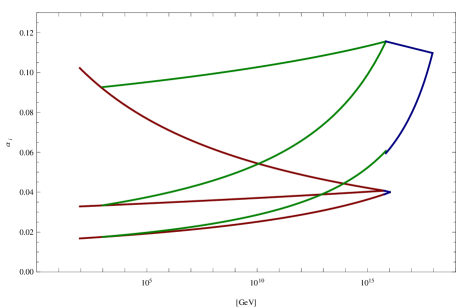
Figure 1: Gauge coupling unification in the minimal (red solid lines) and Type II (green solid lines) flipped $SU(5)\times U(1)_{X}$ models for benchmark scenario $B^{\prime}$. Starting from the top, we depict the gauge couplings $\alpha_{3}$, $\alpha_{2}$, and $\alpha_{Y}$. The discontinuity at $M_{Z}$ (most visible for $\alpha_{3}$) stems from early absorption of the thresholds into a function which is from that scale upward continuous.

In our numerical calculations, we use the weak-scale data in Ref. Amsler:2008zzb , and the top quark mass in Ref. :2009ec . We adopt benchmark scenario $B^{\prime}$ of Ref. Battaglia:2003ab as our reference supersymmetric spectrum, which is near a region of parameter space favored by the $\chi^{2}$ minimization of cumulative deviation from experiments Ellis:2004tc . We present gauge coupling unification for the minimal and Type II flipped $SU(5)\times U(1)_{X}$ models in Fig. 1. We additionally present the $U(1)_{X}$ gauge coupling $g_{1}$ at $M_{23}$, unified $SU(5)$ coupling $g_{23}$, mass scale $M_{23}$, and the proton partial lifetime for the minimal, Type I and Type II models in Table 1. Because of the TeV-scale vector-like particles, we find parity for the gauge couplings $g_{23}$ in the Type I and Type II models, with each coupled significantly more strongly than the minimal model, while $M_{23}$ is slightly larger. Thus, the proton partial lifetime in the Type I and Type II models are shorter than the minimal model by a factor 1/4.3. The central prediction of the proton partial lifetime for the minimal, Type I and Type II models is well below $10^{35}$ years, within the reach of the future Hyper-Kamiokande and DUSEL experiments. However, the uncertainty from heavy threshold corrections ever threatens to undo this promising result.

Model	$g_{1}$	$g_{23}$	$M_{23}$ (GeV)	$\tau_{p}$ (Years)
Minimal	0.70	0.72	$5.8\times 10^{15}$	$4.3\times 10^{34}$
Type I	0.75	1.21	$6.8\times 10^{15}$	$1.0\times 10^{34}$
Type II	0.87	1.20	$6.8\times 10^{15}$	$1.0\times 10^{34}$

Table 1: Gauge couplings $g_{1}$ and $g_{23}$, mass scale $M_{23}$, and proton partial lifetime $\tau_{p}$ in the minimal, Type I and Type II flipped $SU(5)\times U(1)_{X}$ models for benchmark scenario $B^{\prime}$.

Including uncertainties from threshold corrections at the $M_{Z}$ and $M_{23}$ scales, we present the proton partial lifetime in the minimal and Type II flipped $SU(5)\times U(1)_{X}$ models for the process $p\rightarrow e^{+}\pi^{0}$ in Figs. 2 and 3 respectively, for each benchmark scenario from $A^{\prime}$ to $K^{\prime}$ of Ref. Battaglia:2003ab . Central values are depicted by the narrow white gap between red and blue, with the darkend regions on either side showing the error propagated from uncertainty in the $M_{Z}$-scale parameters, combined in quadrature. The lighter blue on the right-hand side depicts plausible variation from the heavy threshold corrections, as in Eq. (10), which can only extend the proton lifetime for flipped $SU(5)\times U(1)_{X}$ models. In the minimal model, the central partial lifetime is in the range of $4-7\times 10^{34}$ years for benchmark scenarios from $A^{\prime}$ to $I^{\prime}$, and about $1-2\times 10^{35}$ years for benchmark scenarios $J^{\prime}$ and $K^{\prime}$. However, the uncertainties from the heavy threshold corrections at $M_{23}$ are indeed quite large. Proton decay appears to be within the reach of the future Hyper-Kamiokande and DUSEL experiments if the heavy threshold corrections are more modest.

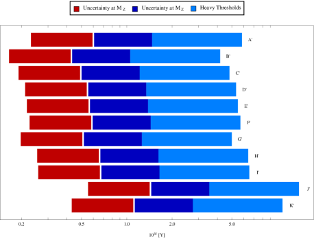
Figure 2: Proton partial lifetime in the unit $10^{35}$ years in the minimal flipped $SU(5)\times U(1)_{X}$ model.

For Type II flipped $SU(5)\times U(1)_{X}$ model, the central values for the partial lifetime are about $1-2\times 10^{34}$ years for benchmark scenarios from $A^{\prime}$ to $I^{\prime}$, and about $2-3\times 10^{34}$ years for benchmark scenarios $J^{\prime}$ and $K^{\prime}$. Even including uncertainties from the light and heavy threshold corrections, the lifetime is still less than $2-3\times 10^{35}$ years for all scenarios considered. A strong majority of the parameter space for proton decay does indeed appear to be within the reach of the future Hyper-Kamiokande and DUSEL experiments for the Type II flipped $SU(5)\times U(1)_{X}$ model. This basic conclusion holds also for the Type I flipped $SU(5)\times U(1)_{X}$ model.

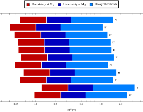
Figure 3: Proton partial lifetime in the unit $10^{35}$ years in the Type II flipped $SU(5)\times U(1)_{X}$ model.

Conclusions – Proton decay is one of the most unique yet ubiquitous predictions of GUTs. We have studied the proton decay process $p\rightarrow e^{+}\pi^{0}$ via dimension six operators from the heavy gauge boson exchange. Including uncertainties from the light and heavy threshold corrections, we have shown that a majority of the parameter space for proton decay is indeed within the reach of the future Hyper-Kamiokande and DUSEL experiments for the Type I and Type II flipped $SU(5)\times U(1)_{X}$ models. The minimal flipped $SU(5)\times U(1)_{X}$ model is also testable if the heavy threshold corrections are small. In particular, detectability of TeV-scale vector-like particles at the LHC presents an opportunity for cross correlation of results between the most exciting particle physics experiments of the coming decade.

Acknowledgments – We would like to thank D. B. Cline for helpful private communication. This research was supported in part by the DOE grant DE-FG03-95-Er-40917 (TL and DVN), by the Natural Science Foundation of China under grant No. 10821504 (TL), and by the Mitchell-Heep Chair in High Energy Physics (TL).

References

- (1) J. R. Ellis, S. Kelley and D. V. Nanopoulos, Phys. Lett. B 260, 131 (1991); P. Langacker and M. X. Luo, Phys. Rev. D 44, 817 (1991); U. Amaldi, W. de Boer and H. Furstenau, Phys. Lett. B 260, 447 (1991).
- (2) H. Nishino et al. [Super-Kamiokande Collaboration], Phys. Rev. Lett. 102, 141801 (2009).
- (3) H. Georgi and S. L. Glashow, Phys. Rev. Lett. 32, 438 (1974).
- (4) S. Dimopoulos and H. Georgi, Nucl. Phys. B 193, 150 (1981).
- (5) H. Murayama and A. Pierce, Phys. Rev. D 65, 055009 (2002), and references therein.
- (6) B. S. Acharya and E. Witten, arXiv:hep-th/0109152.
- (7) E. Witten, arXiv:hep-ph/0201018.
- (8) C. Beasley, J. J. Heckman and C. Vafa, JHEP 0901, 058 (2009); JHEP 0901, 059 (2009).
- (9) R. Donagi and M. Wijnholt, arXiv:0802.2969 [hep-th]; arXiv:0808.2223 [hep-th].
- (10) S. M. Barr, Phys. Lett. B 112, 219 (1982).
- (11) J. P. Derendinger, J. E. Kim and D. V. Nanopoulos, Phys. Lett. B 139, 170 (1984).
- (12) I. Antoniadis, J. R. Ellis, J. S. Hagelin and D. V. Nanopoulos, Phys. Lett. B 194, 231 (1987).
- (13) J. R. Ellis, J. L. Lopez and D. V. Nanopoulos, Phys. Lett. B 371, 65 (1996).
- (14) J. R. Ellis, D. V. Nanopoulos and J. Walker, Phys. Lett. B 550, 99 (2002).
- (15) J. Jiang, T. Li and D. V. Nanopoulos, Nucl. Phys. B 772, 49 (2007).
- (16) J. L. Lopez, D. V. Nanopoulos and K. J. Yuan, Nucl. Phys. B 399, 654 (1993).
- (17) J. Jiang, T. Li, D. V. Nanopoulos and D. Xie, Phys. Lett. B 677, 322 (2009); Nucl. Phys. B 830, 195 (2010).
- (18) K. Nakamura, Int. J. Mod. Phys. A 18, 4053 (2003).
- (19) S. Raby et al., arXiv:0810.4551 [hep-ph].
- (20) T. Li, D. V. Nanopoulos and J. W. Walker, arXiv:1003.2570 [hep-ph].
- (21) G. F. Giudice and A. Masiero, Phys. Lett. B 206, 480 (1988).
- (22) J. J. Heckman and C. Vafa, JHEP 0909, 079 (2009).
- (23) Y. Kuramashi [JLQCD Collaboration], arXiv:hep-ph/0103264.
- (24) M. Battaglia, A. De Roeck, J. R. Ellis, F. Gianotti, K. A. Olive and L. Pape, Eur. Phys. J. C 33, 273 (2004).
- (25) C. Amsler et al. [Particle Data Group], Phys. Lett. B 667, 1 (2008).
- (26) [Tevatron Electroweak Working Group and CDF Collaboration and D0 Collab], arXiv:0903.2503 [hep-ex].
- (27) J. R. Ellis, S. Heinemeyer, K. A. Olive and G. Weiglein, JHEP 0502, 013 (2005).