The effects of opacity on gravitational stability in protoplanetary discs

Abstract

In this paper we consider the effects of opacity regimes on the stability of self-gravitating protoplanetary discs to fragmentation into bound objects. Using a self-consistent 1-D viscous disc model, we show that the ratio of local cooling to dynamical timescales $\Omega t_{\mathrm{cool}}$ has a strong dependence on the local temperature. We investigate the effects of temperature-dependent cooling functions on the disc gravitational stability through controlled numerical experiments using an SPH code. We find that such cooling functions raise the susceptibility of discs to fragmentation through the influence of temperature perturbations – the average value of $\Omega t_{\mathrm{cool}}$ has to increase to prevent local variability leading to collapse. We find the effects of temperature-dependence to be most significant in the ‘opacity gap’ associated with dust sublimation, where the average value of $\Omega t_{\mathrm{cool}}$ at fragmentation is increased by over an order of magnitude. We then use this result to predict where protoplanetary discs will fragment into bound objects, in terms of radius and accretion rate. We find that without temperature dependence, for radii $\lesssim 10AU$ a very large accretion rate $\sim 10^{-3}\;M_{\odot}\;\mathrm{yr}^{-1}$ is required for fragmentation, but that this is reduced to $10^{-4}\;M_{\odot}\;\mathrm{yr}^{-1}$ with temperature-dependent cooling. We also find that the stability of discs with accretion rates $\lesssim 10^{-7}\;M_{\odot}\;\mathrm{yr}^{-1}$ at radii $\gtrsim 50AU$ is enhanced by a lower background temperature if the disc becomes optically thin.

1 Introduction

The formation of planets within protoplanetary discs is a subject that attracts considerable interest, with two main competing schools of thought. The core accretion-gas capture model (Lissauer, 1993; Lissauer & Stevenson, 2007; Klahr, 2008) posits hierarchical growth, with the collisional coagulation of dust grains initially leading to centimetre-sized particles, and thence on to planetesimals and rocky planets. Once a critical mass is reached, it is then possible to accrete a gaseous envelope and hence form giant Jupiter-like planets. Various observations have successfully confirmed this mode of planet formation, for example Marcy et al. (2005), Dodson-Robinson & Bodenheimer (2009).

However, this model cannot explain all the available observations. Kennedy & Kenyon (2008) show that beyond approximately 20 AU, the timescales for giant planet formation via core accretion exceed the expected disc lifetime of approximately 10 Myr, implying that no planets should be detected in this region. However, recent observations of HR8799 with the Keck and Gemini telescopes have produced direct images of giant planets (5 - 13 $M_{\mathrm{J}}$) orbiting at radii of up to $\sim 70$ AU (Marois et al., 2008). Similar observations of other systems (e.g. $\beta$ Pic b (Lagrange et al., 2009) and Formalhuat (Kalas et al., 2008)) and theoretical work on the formation of 2MASS1207b (Lodato et al., 2005) have suggested that there is another mechanism for planet formation at work, and this is thought to be the effect of gravitational instabilities within the protoplanetary discs themselves.

In protoplanetary discs where the self-gravity of the gas is dynamically important, direct gravitational collapse of locally Jeans-unstable over-densities within the disc (Boss, 1997, 1998; Durisen et al., 2007) would also produce giant planets very rapidly, on the local dynamical timescale. A similar process of gravitational instability leading to local collapse is a strong candidate for the formation of stellar discs around Active Galactic Nuclei (AGN) (Nayakshin et al., 2007) and those observed in our own Galactic Centre (Levin & Beloborodov, 2003; Nayakshin & Cuadra, 2005), and in the context of protostellar discs may furthermore be responsible for the formation of brown dwarves and other low mass stellar companions (Stamatellos et al., 2007a).

The emergence of the gravitational instability within a disc is governed by the parameter $Q$ (Toomre, 1964), which for a gaseous Keplerian disc is given by

$$Q=\frac{c_{\mathrm{s}}\Omega}{\pi G\Sigma}.$$ (1)

This encapsulates the balance between the stabilising effects of rotation ($\Omega(R)$ is the angular frequency at radius $R$) and thermal pressure ($c_{\mathrm{s}}(R)$ is the sound speed) and the destabilising effect of the disc self-gravity via the surface density $\Sigma(R)$. When $Q\lesssim 1$ the instability is initiated, leading to the presence of spiral density waves within the disc which, depending on the local cooling rate, may persist in a self-regulated quasi-stable state (Gammie, 2001; Lodato & Rice, 2004) or may fragment into bound clumps (Johnson & Gammie, 2003; Rice et al., 2005). Discs that are sufficiently cool are therefore expected to be susceptible to the gravitational instability, and it is thought that at least in the early stages of stellar evolution, many discs enter the self-gravitating phase (Hartmann, 2009).

Once the gravitational instability is initiated, heat is input to the disc on the dynamical timescale through the passage of spiral compression/shock waves (Cossins et al., 2009). Various numerical studies using both 2D and 3D models of self-gravitating discs have produced the result that, in order to induce fragmentation, the disc must be able to cool on a timescale faster than a few times the local dynamical time, $t_{\mathrm{dyn}}=\Omega^{-1}$ (Gammie, 2001; Rice et al., 2005). This condition is likely to occur only at relatively large radii ($\sim 100$ AU), on the assumption that stellar or external irradiation of the disc is negligible (Rafikov, 2009; Stamatellos & Whitworth, 2009b).

These models have generally used a cooling rate prescribed by using a fixed ratio between the local cooling ($t_{\mathrm{cool}}$) and dynamical ($\Omega^{-1}$) times, such that

$$\Omega t_{\mathrm{cool}}=\beta$$ (2)

for some constant $\beta$ throughout the radial extent of the disc. Various authors (e.g. Gammie 2001; Rice et al. 2005) have found that fragmentation occurs whenever $\Omega t_{\mathrm{cool}}\approx 3-7$. By using a more realistic cooling framework based on the optical depth, Johnson & Gammie (2003) found that the fragmentation boundary (defined hereafter as the ratio of the cooling to dynamical timescales, $\Omega t_{\mathrm{cool}}$ at fragmentation) may in fact be over an order of magnitude greater than this, leading to an enhanced tendency towards fragmentation. This variation in $\Omega t_{\mathrm{cool}}$ they ascribed to the implicit dependence of the cooling function on the disc opacity, and hence on temperature.

Using the opacity tables of Bell & Lin (1994) it is clear that the opacity is a strong function of temperature in certain regimes, and by modelling protoplanetary discs as optically thick in the Rosseland mean sense, $\Omega t_{\mathrm{cool}}$ shows power law dependencies on both the local temperature and density. In cases where this dependence is strong, it is therefore possible that small temperature fluctuations may push the local value of $\Omega t_{\mathrm{cool}}$ below the fragmentation boundary, even when the average value is significantly above it.

In this paper we therefore seek to investigate and clarify the exact relationship between the fragmentation boundary and the temperature dependence of $\Omega t_{\mathrm{cool}}$, using a Smoothed Particle Hydrodynamics (sph) code to conduct global, 3D numerical simulations of discs where the cooling time follows a power-law dependence on the local temperature. In addition, various studies have shown that in a quasi-steady state the gravitational instability may be modelled pseudo-viscously (Lodato & Rice 2005; Cossins et al. 2009; Clarke 2009; Rafikov 2009). We therefore use the $\alpha$-prescription of Shakura & Sunyaev (1973) and the assumption of local thermal equilibrium, where

$$\Omega t_{\mathrm{cool}}=\frac{4}{9}\frac{1}{\gamma(\gamma-1)\alpha}$$ (3)

and $\gamma$ is the ratio of specific heats, to construct an analytical model of the opacity regimes present within a marginally gravitationally stable disc. From this we can therefore predict analytically if and where such discs would become prone to fragmentation, and also compare these results to those from the more complex simulations where radiative transfer is modelled, such as Boley (2009) and Stamatellos & Whitworth (2009b).

The structure of this paper is therefore as follows. In Section 2 we discuss some of the theoretical results relevant to protoplanetary discs, and introduce a simplified cooling function derived from the various opacity regimes. We further consider the effects we expect these cooling prescriptions to have on the susceptibility of protoplanetary discs to fragmentation. In Section 3 we briefly outline the numerical modelling techniques used in our simulations and detail our initial conditions. In Section 4 we present the results from these simulations, before proceeding to collate these with the analytical predictions in Section 5. Finally in Section 6 we discuss the ramifications of our work and the conclusions that may be drawn from it.

2 Theoretical Results

In this section we derive analytical results for the dependence of the cooling timescale $t_{\mathrm{cool}}$ on temperature and density, such as we might expect to find in a quasi-gravitationally stable protoplanetary disc environment. We also consider analytically the effects that a (specifically) temperature dependent cooling time will have on the stability of such a disc to fragmentation.

2.1 $\Omega t_{\mathrm{cool}}$ in the Optically Thick Regime

As in the case of Gammie (2001), we may start from the following basic equations:

$$t_{\mathrm{cool}} = \frac{U\Sigma}{\Lambda},$$ (4)

$$\tau \approx \rho H\kappa,$$ (5)

$$\Sigma = 2\rho H,$$ (6)

$$c_{\mathrm{s}}^{2} = \frac{\gamma\mathcal{R}T}{\mu},$$ (7)

where $U$ is the specific internal energy, $\Lambda$ is the cooling rate per unit area, $\tau$ is the optical depth, $\rho$ is the (volume) density, $H=c_{\mathrm{s}}/\Omega$ is the disc scale height, $\kappa$ is the opacity, $\gamma$ is the ratio of specific heats, $\mathcal{R}=k/m_{\mathrm{H}}$ is the universal gas constant ($k$ being the Boltzmann constant and $m_{\mathrm{H}}$ the mass of a hydrogen atom), $T$ is the local mid-plane temperature and $\mu$ is the mean molecular weight of the gas. Note that the factor of two in equation 6 arises from there being two faces of the disc from which to radiate.

In the case where the disc is optically thick (in terms of the Rosseland mean), then the cooling rate per surface area $\Lambda$ may be given as

$$\Lambda=\frac{16\sigma T^{4}}{3\tau},$$ (8)

where $\sigma$ is the Stefan-Boltzmann constant. We note that this is strictly valid only in the case where energy is transported radiatively within the disc — convective transport or stratification within the disc will alter this relationship (see for example Rafikov 2007). For the purely radiative case, the vertical temperature structure of the disc is therefore accounted for via this formalism, and is characterised by the midplane temperature $T$ and the optical depth $\tau$. In order to prevent divergence of this cooling function at low optical depths and to interpolate smoothly into the optically thin regime, others including Johnson & Gammie (2003) and Rice & Armitage (2009) have used a cooling function of the form

$$\Lambda=\frac{16\sigma T^{4}}{3}\left(\tau+\frac{1}{\tau}\right)^{-1},$$ (9)

which becomes directly proportional to the optical depth in the optically thin limit. In general however, we find that discs only become optically thin at large radii, and that this correction is therefore only relevant to the case where the cooling is dominated by ices.

Furthermore, we note that for systems where the stellar mass dominates over that of the disc, the density $\rho$ may be approximated by

$$\rho\approx\frac{M_{*}}{2\pi R^{3}Q}$$ (10)

where $M_{*}$ is the mass of the central star and $R$ the radial distance from the central star, and therefore we have $\Omega^{2}=2\pi G\rho Q$ in the case of Keplerian rotation, with $G$ being the universal gravitation constant. Recalling also that $c_{\mathrm{s}}^{2}=U\gamma(\gamma-1)$, equations 4 – 10 may be rearranged to show that in the optically thick case, the ratio of cooling to dynamical times should be

$$\Omega t_{\mathrm{cool}}=\frac{3\mathcal{R}^{2}}{8\sigma\sqrt{2\pi G}}\frac{\gamma}{\gamma-1}\frac{\kappa}{\mu^{2}}\;Q^{-1/2}\;\rho^{3/2}\;T^{-2}.$$ (11)

Bell & Lin (1994) found that the opacity can be reasonably well approximated by power-law dependencies on temperature and density, such that

$$\kappa=\kappa_{0}\;\rho^{a}\;T^{b}.$$ (12)

Specific values of $a$, $b$ and $\kappa_{0}$ apply for each opacity regime, such that the value of $\kappa$ varies continuously over the regime boundaries. Using these approximations, we find that the $\Omega t_{\mathrm{cool}}$ value for the various opacity regimes can be given by

$$\Omega t_{\mathrm{cool}}=\frac{3\mathcal{R}^{2}}{8\sigma\sqrt{2\pi G}}\frac{\gamma\kappa_{0}}{\mu^{2}(\gamma-1)}\;Q^{-1/2}\;\rho^{a+3/2}\;T^{b-2}.$$ (13)

For each opacity regime, the constant $\kappa_{0}$, the exponents $a$ and $b$, the transition temperatures between the regimes and the functional dependence of $\Omega t_{\mathrm{cool}}$ on temperature and density are given in Table 1. It should be noted that for the purposes of these tables the temperature and density should be measured in cgs units.

Table 1: Details of the various optical regimes by type, showing the transition temperatures and the functional dependence of $\Omega t_{\mathrm{cool}}$ on the temperature and density in the optically thick regime. Note that all values are quoted in cgs units. See Bell & Lin (1994) for further details.

Opacity Regime	$\mathbf{\kappa_{0}}$ (cm2 g-1)	$\mathbf{a}$	$\mathbf{b}$	Temperature Range ($\mathbf{K}$)		Dependence of $\Omega t_{\mathrm{cool}}$
				From	To
Ices	$2\times 10^{-4}$	0	2	0	$166.810$	$\rho^{3/2}$
Sublimation of Ices	$2\times 10^{16}$	0	-7	$166.810$	$202.677$	$\rho^{3/2}\;T^{-9}$
Dust Grains	$1\times 10^{-1}$	0	1/2	$202.677$	$2286.77\;\rho^{2/49}$	$\rho^{3/2}\;T^{-5/2}$
Sublimation of Dust Grains	$2\times 10^{81}$	1	-24	$2286.77\;\rho^{2/49}$	$2029.76\;\rho^{1/81}$	$\rho^{5/2}\;T^{-26}$
Molecules	$1\times 10^{-8}$	2/3	3	$2029.76\;\rho^{1/81}$	$10000.0\;\rho^{1/21}$	$\rho^{13/6}\;T^{1}$
Hydrogen scattering	$1\times 10^{-36}$	1/3	10	$10000.0\;\rho^{1/21}$	$31195.2\;\rho^{4/75}$	$\rho^{11/6}\;T^{8}$
Bound-Free & Free-Free	$1.5\times 10^{20}$	1	-5/2	$31195.2\;\rho^{4/75}$	$1.79393\times 10^{8}\;\rho^{2/5}$	$\rho^{5/2}\;T^{-9/2}$
Electron scattering	0.348	0	0	$1.79393\times 10^{8}\;\rho^{2/5}$	——–	$\rho^{3/2}\;T^{-2}$

2.2 Effects of Temperature Dependence on Fragmentation

We now specifically consider the effects of temperature fluctuations on the stability of a disc to fragmentation, using a simplified cooling prescription derived from a consideration of equation 13.

In the previous section it was noted that the ratio of the local cooling and dynamical times $\Omega t_{\mathrm{cool}}$ has a direct dependence on the local mid-plane temperature $T$. Given that (from Table 1) this dependence is generally much stronger than that on density, it is physically reasonable to consider a simplified cooling function where we only include the effects of temperature, and where we define the cooling time via the relationship

$$\Omega t_{\mathrm{cool}}=\beta\left(\frac{T}{\bar{T}}\right)^{-n},$$ (14)

for some general value of the cooling exponent $n$ and cooling parameter $\beta$. Here $\bar{T}$ is the azimuthally averaged mid-plane temperature $T$ in thermal equilibrium, and thus we see that when thermal equilibrium is reached, the average cooling timescale is expected to reduce to $\left<\Omega t_{\mathrm{cool}}\right>\approx\beta$, with a fragmentation boundary $\beta_{n}$ associated with each value of $n$. In particular, with $n=0$, at fragmentation we have $\Omega t_{\mathrm{cool}}=\left<\Omega t_{\mathrm{cool}}\right>=\beta_{0}$, which Gammie (2001), Rice et al. (2005) and others have found to be in the range $3-7$.

In the case of temperature dependent cooling (where $n\neq 0$), if the equilibrium value of the cooling parameter $\beta>\beta_{0}$, the disc may still fragment due to temperature fluctuations leading to a short term (relative to the dynamical timescale) decrease in the instantaneous value of $\beta$ to less than the threshold value. For a power-law index $n$, in order to calculate the value $\beta_{n}$ of the equilibrium cooling parameter below which fragmentation occurs, we make the assumption that fragmentation takes place wherever the instantaneous value of $\Omega t_{\mathrm{cool}}$ is held at or below the critical value $\beta_{0}$ for longer than a dynamical time, independent of the mechanism by which the cooling is effected. If we therefore consider temperature fluctuations such that $T=\bar{T}+\delta T$, we find that at the fragmentation boundary

$$\beta_{0}=\beta_{n}\left(1+\frac{\delta T}{\bar{T}}\right)^{-n}.$$ (15)

In Cossins et al. (2009) for the case where $M_{\mathrm{disc}}/M_{*}=0.1$ we found that on average the strength of the surface density perturbations $\delta\Sigma/\bar{\Sigma}$ can be linked to the strength of the cooling through the following relationship,

$$\left<\frac{\delta\Sigma}{\bar{\Sigma}}\right>\approx\frac{1}{\left<\Omega t_{\mathrm{cool}}\right>^{1/2}},$$ (16)

where angle brackets denote the RMS value. In a similar manner we may say that

$$\left<\frac{\delta T}{\bar{T}}\right>=\frac{k}{\left<\Omega t_{\mathrm{cool}}\right>^{1/2}},$$ (17)

where $k$ is to be defined empirically. At fragmentation therefore we have

$$\left<\frac{\delta T}{\bar{T}}\right>=\frac{k}{\beta_{n}^{1/2}},$$ (18)

noting that by construction for a given index $n$, at fragmentation $\left<\Omega t_{\mathrm{cool}}\right>=\beta_{n}$. Combining this with equation 15 we find that in the case where the cooling is allowed to vary with temperature as per equation 14, the fragmentation boundary $\beta_{n}$ satisfies the following equation;

$$\beta_{0}=\beta_{n}\left(1+\frac{k}{\beta_{n}^{1/2}}\right)^{-n}.$$ (19)

This implicit equation can therefore be solved to find the value of the fragmentation boundary $\beta_{n}$ for all $n\gtrsim-2$ (below this $\beta_{n}$ becomes undefined), as shown later in Table 4.

3 Numerical Set Up

3.1 The SPH code

All of the simulations presented hereafter were performed using a 3D smoothed particle hydrodynamics (sph) code, a Lagrangian hydrodynamics code capable of modelling self-gravity (see for example, Benz 1990, Monaghan 1992). The code self-consistently incorporates the so-called $\nabla h$ terms to ensure energy conservation, as described in Springel & Hernquist (2002), Price & Monaghan (2007). All particles evolve according to individual time-steps governed by the Courant condition, a force condition (Monaghan, 1992), an integrator limit (Bate et al., 1995) and an additional condition that ensures the local timestep is always less than the local cooling time.

We have modelled our systems as a single point mass (onto which gas particles may accrete if they enter within a given sink radius and satisfy certain boundness conditions — see Bate et al. 1995) orbited by 500,000 sph gas particles; a set up common to many other sph simulations of such systems (e.g. Rice et al. (2003); Lodato & Rice (2004, 2005); Clarke et al. (2007); Cossins et al. (2009)) but at a higher resolution than most. The central object is free to move under the gravitational influence of the disc.

In common with many other simulations where cooling is being investigated (Gammie (2001); Lodato & Rice (2005); Cossins et al. (2009) for example) we use a simple implementation of the following form;

$$\frac{du_{{i}}}{dt}=-\frac{u_{i}}{t_{\mathrm{cool},i}},$$ (20)

where $u_{i}$ and $t_{\mathrm{cool},i}$ are the specific internal energy and cooling time associated with each particle respectively. The cooling time is allowed to vary with the particle temperature $T_{i}$ in such a manner that

$$\Omega_{i}t_{\mathrm{cool},i}=\hat{\beta}\left(\frac{T_{i}}{\bar{T}}\right)^{-n},$$ (21)

where $\Omega_{i}$ is the angular velocity of the particle, $\bar{T}$ is the equilibrium temperature, and $\hat{\beta}$ and $n$ are input values held constant throughout any given simulation. Given that $T\sim c_{\mathrm{s}}^{2}$, equation 1 shows that for a given value of the surface density $\Sigma$ this is equivalent to

$$\Omega_{i}t_{\mathrm{cool},i}=\hat{\beta}\left(\frac{Q_{i}}{\bar{Q}}\right)^{-2n},$$ (22)

where again $Q_{i}$ is the value of the $Q$ parameter evaluated at each particle, and $\bar{Q}$ is the expected equilibrium value of $Q$, which we take to be 1 throughout. Note that a priori we do not know exactly what the equilibrium value of $Q$ will be once the gravitational instability has saturated. Indeed as we shall see this turns out to be slightly greater than unity, but still such that $Q\approx 1$. The effective value of the cooling parameter is given by

$$\beta=\hat{\beta}Q^{-2n},$$ (23)

where $Q$ is the actual value to which the simulations settle. Since we are exploring relatively large values of $n$, $\beta$ can vary significantly from our input value $\hat{\beta}$ for even small changes in $Q$.

Finally we calculate the equivalent surface density $\Sigma_{i}$ (and thus $Q_{i}$) at the radial location of each particle $R_{i}$ by dividing up the disc into (cylindrical) annuli, calculating the surface density for each annulus, and then interpolating radially to obtain $\Sigma_{i}(R_{i})$. To prevent boundary effects, for simulations where $n>1.0$ the temperature dependent effects are limited to an annulus $15\leq R\leq 20$ (in code units — note that initially $R_{\mathrm{in}}=0.25$ and $R_{\mathrm{out}}=25.0$). At other radii we keep $\Omega t_{\mathrm{cool}}=8$, a value chosen to suppress fragmentation in regions outside the annulus of interest (see for instance Alexander et al. 2008).

All simulations have been run with the particles modelled as a perfect gas, with the ratio of specific heats $\gamma=5/3$. Heat addition is allowed for via $P\mathrm{d}V$ work and shock heating. Artificial viscosity has been included through the standard sph formalism, with $\alpha_{\mathrm{SPH}}=0.1$ and $\beta_{\mathrm{SPH}}=0.2$ — although these values are smaller than those commonly used in sph simulations, this limits the transport and heating induced by artificial viscosity. As shown in Lodato & Rice (2004), with this choice of parameters the transport of energy and angular momentum due to artificial viscosity is a factor of 10 smaller than that due to gravitational perturbations, while we are still able to resolve the weak shocks occurring in our simulations.

By using the cooling prescription outlined above in equation 22, the rate at which the disc cools is governed by the dimensionless parameters $Q$, $\hat{\beta}$ and $n$, and the cooling is thereby implemented scale free. The governing equations of the entire simulation can therefore likewise be recast in dimensionless form. In common with the previous sph simulations mentioned above, we define the unit mass to be that of the central object – the total disc mass and individual particle masses are therefore expressed as fractions of the central object mass. We can self-consistently define an arbitrary unit (cylindrical) radius $R_{0}$, and thus, with $G=1$, the unit timestep is the dynamical time $t_{\mathrm{dyn}}=\Omega^{-1}$ at radius $R=1$.

3.2 Initial conditions

All our simulations model a central object of mass $M_{*}$, surrounded by a gaseous disc of mass $M_{\mathrm{disc}}=0.1M_{*}$. We have used an initial surface density profile $\Sigma\sim R^{-3/2}$, which implies that in the marginally stable state where $Q\approx 1$, the disc temperature profile should be approximately flat for a Keplerian rotation curve. Since the surface density evolves on the viscous time $t_{\mathrm{visc}}\gg t_{\mathrm{dyn}}=\Omega^{-1}$ this profile remains roughly unchanged throughout the simulations. Radially the disc extends from $R_{\mathrm{in}}=0.25$ to $R_{\mathrm{out}}=25.0$, as measured in the code units described above. The disc is initially in approximate hydrostatic equilibrium in a Gaussian distribution of particles with scale height $H$. The azimuthal velocities take into account both a pressure correction (Lodato, 2007) and the enclosed disc mass. In both cases, any variation from dynamical equilibrium is washed out on the dynamical timescale.

The initial temperature profile is $c_{\mathrm{s}}^{2}\sim R^{-1/2}$ and is such that the minimum value of the Toomre parameter $Q_{\mathrm{min}}=2$ occurs at the outer edge of the disc. In this manner the disc is initially gravitationally stable throughout. Note that the disc is not initially in thermal equilibrium – heat is not input to the disc until gravitational instabilities are initiated.

3.3 Simulations run

Since our simulations use a slightly different surface density profile to that used by previous authors ($\Sigma\sim R^{-3/2}$, cf. $\Sigma\sim R^{-1}$ in Rice et al. 2005, $\Sigma\sim R^{-7/4}$ in Rice et al. 2003) we initially ran five simulations at various values of $\beta$ with the cooling exponent $n$ set equal to zero, to find the fragmentation boundary in the case where the cooling is independent of temperature. Thereafter, simulations were run at various $\beta$ values as $n$ was incremented up to $n=3$, to ascertain the fragmentation boundary in each case. A summary of all the simulations run is given in Table 2.

Table 2: Table of simulations run for various values of the cooling exponent $n$ and rate $\beta$. Note that since many of these simulations were run concurrently, there is a degree of overlap in the $\beta$ values used.

Exponent ($n$)	Input cooling parameter ($\hat{\beta}$)
0.0	3, 4, 4.5, 5, 6
0.5	4, 4.5, 5, 5.5, 6
1.0	3, 4, 5, 6, 7, 8, 9, 10
1.5	7, 8, 9, 10, 11
2.0	10, 11, 12, 13, 14, 15, 16, 17, 18
3.0	20, 22.5, 25, 27.5, 30, 32.5, 35, 37.5, 40

4 Simulation Results

4.1 Detecting Fragmentation

First of all it is useful to explain how fragmentation has been detected in our simulations. Throughout all the numerical simulations run, the maximum density over all particles has been tracked as a function of elapsed time. In the case of a non-fragmenting disc, the maximum always occurs at the inner edge of the disc (as would be expected), and is relatively stable over time. However, once a fragment forms, this maximum density (now corresponding to the radius at which the fragment forms) rises exponentially, on its own dynamical timescale. An example is shown in Fig. 1, and the various changes in gradient correspond to various fragments at different radii (and thus with differing growth rates) achieving peak density. A similar increase in the central density of proto-fragments is observed in Stamatellos & Whitworth (2009a), although the timescales differ due to the use of different equations of state.

This rise in the maximum density has therefore been used throughout as a tracer of fragment formation, and the evolution has been followed until the fragments are at least four orders of magnitude greater than the original peak density.

Figure 1: Maximum density plot showing the characteristic rise due to fragment formation, seen here for the simulation where $\beta=4.0$, $n=0$ (where the cooling is independent of temperature). There is clear evidence of fragment formation at $t\approx 20,000$, with both density and time being shown in code units.

4.2 Averaging Techniques

Throughout the following analysis, we have defined the average value of a (strictly positive) quantity, which we denote by an overbar, as the geometric mean of the particle quantities. The reason for this is we find that in the “gravo-turbulent” equilibrium state properties such as the temperature, density and Q value are log-normally distributed. This is shown for example in Fig. 2, where the temperature data from the simulation match a predicted log-normal distribution to within one percent. (Note the reduced radial range to reduce the effect of the inherent gradual reduction in temperature with radius.) The geometric mean being precisely equivalent to the exponential of the arithmetic mean of the logged values, this process recovers the mean value of the normal distribution of $\ln T$.

Figure 2: Distribution of particle temperatures for $16.25\leq R\leq 18.75$, and a predicted log-normal distribution based on the same data. The two are equal to within approximately 1%.

Similarly, to calculate the perturbation strengths (e.g $\delta A/\bar{A}$ for some quantity $A$) we note that

$$\frac{\delta A}{\bar{A}}\approx\frac{\mathrm{d}A}{A}=\mathrm{d}\ln A.$$ (24)

The RMS value of $\delta A/\bar{A}$ is then equivalent to the standard deviation of $\ln A$, which again can be recovered directly from the log-normal distribution. Referring again to Fig. 2 we therefore see that $\bar{T}=10^{-4.498}=3.177\times 10^{-5}$ (in code units), and that $\delta T/\bar{T}=\sigma=0.348$.

4.3 Equilibrium States

First of all, we need to determine the exact value of the fragmentation boundary in the case where $n=0$ (and thus where $\beta=\hat{\beta}$), which we denote by $\beta_{0}$. As seen in Table 2, simulations were run at various values $3.0\leq\beta\leq 6.0$, and we find that the boundary lies between 4.0 and 4.5. We therefore take the critical value as being the midpoint, such that $\beta_{0}=4.25$.

Continuing with the $n=0$ case, we find throughout that the value of $Q$ to which the simulations settle is slightly above unity. The steady state values (time averaged over 1000 timesteps) are shown for various $\beta$ values in Fig. 3, and we see that the average $Q$ value is approximately 1.091, where we have averaged over both $\beta$ and radius (where $15\leq R\leq 20$, for comparison with simulations with higher $n$). We further note that there is scatter of $\sim 10\%$ about this average, and (although not shown) this is equally true of the simulations where $n>0$.

Figure 3: Plot of $Q$ against radius for various values of $\beta$ in the temperature independent case $n=0$. For the fragmenting cases ($\beta<4.25$) the values shown are from immediately prior to fragmentation.

Note then that for large $n$ the effective value of the cooling parameter $\beta$ at any given radius may be substantially different from the numerical input value $\hat{\beta}=\beta Q^{2n}$ (see equation 23) that we use to characterise the cooling law. In order to determine the fragmentation boundary with any accuracy, we therefore need to consider the true value of $\beta$ rather than the input value $\hat{\beta}$.

4.4 Cooling Strength and Temperature Fluctuations

In order to characterise the fragmentation boundary, it is necessary that we validate the assumption encompassed by equation 17, that the temperature perturbation strength is correlated to that of the applied cooling. Using the method outlined above in section 4.2, for each simulation we can calculate azimuthally averaged RMS values for the strength of the temperature fluctuations, which we denote by $\left<\delta T/\bar{T}\right>$. Where $n=0$, these temperature perturbations are plotted as a function of radius for various values of $\beta$ in Fig. 4, where we see that there is a systematic decrease in the perturbation strength with increasing $\beta$, and also that the perturbation strength is almost constant with radius across the self-regulating region ($5\lesssim R\lesssim 25$) of the disc. Using equation 17 we can therefore calculate an empirical value for $k$, and hence averaging both radially (for $15\leq R\leq 20$ as before) and over the available values of $\beta$ we find $k=1.170$ where $n=0$.

Figure 4: Plot showing the strength of temperature perturbations within the disc as a function of radius and $\beta$ for the temperature independent case, where $n=0$.

Furthermore, we note that in the temperature dependent case (where $n\neq 0$), by construction the average value $\left<\Omega t_{\mathrm{cool}}\right>$ is simply the effective value of the cooling strength, $\beta$. We can therefore calculate the value of $k$ for cases where $n\neq 0$, and we find that again $k$ remains constant both with the index $n$ and with radius. Hence we take the value of $k$ to be 1.170, as in the $n=0$ case, and empirically we may therefore say that on average

$$\left<\frac{\delta T}{\bar{T}}\right>=\frac{1.170}{\sqrt{\beta}},$$ (25)

for all $n$.

4.5 The Fragmentation Boundary

We are now in a position to predict empirically the fragmentation boundary in the case where $n\neq 0$, and to compare this directly with the results of our simulations. Table 3 shows the fragmentation boundary $\beta_{n}$ as obtained from our simulations, where once again it is taken as the average of the highest fragmenting and lowest non-fragmenting values of $\beta$ simulated. We find that as expected, there is indeed a rise in the fragmentation boundary as the dependence of the cooling on temperature increases. This variation of the fragmentation boundary is shown against the cooling exponent $n$ in Fig. 5, (where the error bars show the upper and lower bounds from Table 3) along with predicted values generated using the following empirically defined implicit relationship

$$\beta_{0}=\beta_{n}\left(1+\frac{1.170}{\sqrt{\beta_{n}}}\right)^{-n},$$ (26)

where we have used $\beta_{0}=4.25$. Clear from this plot is the fact that the predictions are a very good match to the data observed, and our theoretical model, in which the increased tendency for fragmentation is due to the effects of temperature fluctuations on the cooling rate, is therefore valid. The transition zone shown is bounded by curves corresponding to predictions using $\beta_{0}=4.00$ and $4.50$, the upper and lower bounds for $\beta_{0}$ we obtained through our simulations.

Table 3: Table showing the fragmentation boundaries obtained from the simulations. The central columns show respectively the highest fragmenting and lowest non-fragmenting values of $\beta$ simulated, with $\beta_{n}$ being the midpoint of these. Throughout, $\beta$ is calculated using equation 23.

Exponent ($n$)	Effective cooling rate ($\beta$)		$\beta_{n}$
	Fragmenting	Non-Fragmenting
0.0	4.000	4.500	4.250
0.5	4.825	5.263	5.044
1.0	5.915	6.654	6.284
1.5	6.949	7.644	7.296
2.0	8.458	9.022	8.740
3.0	10.051	11.056	10.554

Figure 5: Plot of $\beta_{n}$ at fragmentation for various values of $n$. The error bars correspond to the greatest non-fragmenting and smallest fragmenting values of $\beta$ found in the simulations, and the cross-hatched transition region represents uncertainty in the exact value of $\beta_{0}$. Note also that where $n<0$ discs may become thermally unstable.

4.6 Statistical Analysis

The effects of temperature perturbations on the fragmentation boundary can be neatly illustrated statistically, if we assume that the distribution of temperatures about the geometric mean $\ln\bar{T}$ is log-Normal (as found in our simulations). Using standard notation we can therefore say that

$$\ln T\sim N(\ln\bar{T},\sigma^{2}),$$ (27)

with standard deviation $\sigma$. By taking logs of equation 14 we further see that

$$\ln\Omega t_{\mathrm{cool}}=\ln\beta-n\ln T+n\ln\bar{T}.$$ (28)

A standard property of the Normal distribution is that for a Normally distributed random variable $X\sim N(\mu,\sigma^{2})$, the distribution of $aX+b$ is given by $N(a\mu+b,a^{2}\sigma^{2})$. Hence from equation 28 we see that the distribution of $\ln\Omega t_{\mathrm{cool}}$ at fragmentation is such that

$$\ln\Omega t_{\mathrm{cool}}\sim N(\ln\beta_{n},n^{2}\sigma^{2}),$$ (29)

i.e., the distribution of $\ln\Omega t_{\mathrm{cool}}$ is centred around $\ln\beta_{n}$ for all $n$, reducing to a $\delta$-function in the limit where $n$ becomes zero and becoming more spread out as $n$ becomes large. Thus in order to counteract the increased width of the distribution, and thus the increased fraction of the gas that is below the fragmentation threshold, the average must rise. This is clearly illustrated in Fig. 6, for values of $n$ between 0 and 4, and where $\beta_{n}$ is given in each case by equation 26 with $\beta_{0}=4.25$.

Figure 6: Variation in the distribution of $\ln\Omega t_{\mathrm{cool}}$ as a function of $n$, clearly showing the increasing width of the distribution with increasing $n$. Note that in the case where $n=0$ the distribution reduces to a $\delta$-function.

5 Opacity-Based Analytic Disc Models

Having quantified the effects of a temperature-dependent cooling law on the fragmentation boundary of protoplanetary discs, we are now in a position to use the known cooling laws for each opacity regime (as given by equation 13) to determine the dominant cooling mechanisms throughout the radial range. We can therefore also use this to re-evaluate the regions of such discs that are unstable to fragmentation, in a similar manner to the analysis undertaken by Clarke (2009).

In order to do this in a physically realistic manner we must also take into account the effects of the magneto-rotational instability (MRI), which operates when the disc becomes sufficiently ionised. Considering only thermal ionisation, we assume that the MRI becomes active when the disc temperature rises above $1000K$ (Clarke, 2009). Although estimates of the viscosity provided through this instability vary (see King et al. (2007) for a summary), numerical simulations suggest it should be in the range $0.001\lesssim\alpha_{\mathrm{MRI}}\lesssim 0.01$ (Winters et al., 2003; Sano et al., 2004). We therefore assume that the MRI is the dominant instability in the disc wherever $T>1000K$ and the $\alpha$ delivered by the gravitational instability falls below 0.01.

To obtain the disc temperature, we note that equations 3, 7, 10, 11 and 12 self-consistently allow the disc properties to be evaluated for any given stellar mass $M_{*}$, mass accretion rate $\dot{M}$ and radius $R$, when combined with the relation

$$\dot{M}=\frac{3\alpha c_{\mathrm{s}}^{3}}{GQ}$$ (30)

(see for instance Clarke 2009; Rafikov 2009; Rice & Armitage 2009). We can thus derive the dependence of the disc temperature $T$ on $Q$, $M_{*}$, $R$ and $\dot{M}$, such that

$$T=\left[\frac{32\sigma}{9\kappa_{0}}\left(\frac{2\pi\mu}{G\gamma\mathcal{R}}\right)^{\frac{1}{2}}\left(\frac{M_{*}}{2\pi}\right)^{-(a+\frac{3}{2})}Q^{a+1}R^{3a+\frac{9}{2}}\dot{M}^{-1}\right]^{\frac{2}{2b-7}}.$$ (31)

Finally, in order to prevent the temperature becoming too low, we assume a fiducial background temperature for the interstellar medium (ISM) of $10K$ (D’Alessio et al., 1998; Hartmann et al., 1998). In this case, we no longer assume that equation 3 holds, as there is additional heating from the background as well as from the gravitational instability.

Since there is a strong dependence on temperature in certain opacity regimes (see Table 1) it is important that the equation of state adequately captures the correct behaviour of both the ratio of specific heats $\gamma$ and the mean molecular weight $\mu$, as variation in these can have significant effects on the system overall. To implement the equation of state we therefore make the assumption that the gas phase of the disc contains only hydrogen and helium, in the ratio $70\colon 30$. We can make this assumption because although the metallicity of the disc is important for the opacity (and thus the cooling), it makes very little contribution to the equation of state. Furthermore, the ratio of ortho- to para-hydrogen is assumed to be held constant at $3\colon 1$. Following on from the analysis of Black & Bodenheimer (1975), Stamatellos et al. (2007b) produced tabulated values of $\rho,T,\gamma$ and $\mu$ for this equation of state and it is these values that we have used throughout. The variation of $\gamma$ with both temperature and density is shown in Fig. 7 – for the variation of the mean molecular weight $\mu$ the reader is referred to Stamatellos et al. (2007b) and Forgan et al. (2009).

Figure 7: Plot showing the variation of the ratio of specific heats $\gamma$ as a function of temperature and density. The density corresponds to the quoted radii for a $Q=1$ disc about a 1 $M_{\odot}$ star. Note that the inverse function for temperature in terms of $\gamma$, $T(\gamma,\rho)$ is multi-valued.

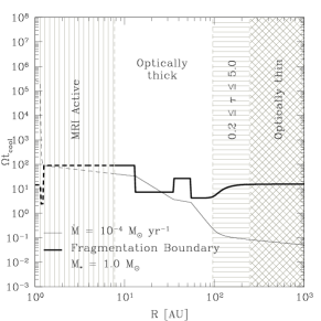
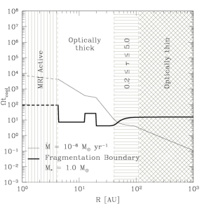
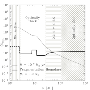
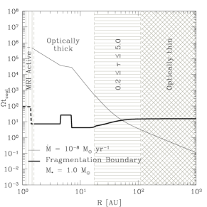
Figure 8: Value of $\Omega t_{\mathrm{cool}}$ as a function of radius for accretion rates of $10^{-4}$ (top left), $10^{-6}$ (top right), $10^{-7}$ (bottom left) and $10^{-8}$ (bottom right) $\;M_{\odot}\;\mathrm{yr}^{-1}$, for a disc about a $1M_{\odot}$ star. The unshaded regions are optically thick ($\tau>5$), the horizontally shaded areas are transitional ($0.2<\tau\leq 5$) and the cross-hatched regions are optically thin ($\tau<0.2$). The vertically shaded areas denote regions of the disc that are MRI active. The disc is stable against fragmentation wherever the value of $\Omega t_{\mathrm{cool}}$ is greater than the fragmentation boundary (shown by the heavy solid line). The dotted lines show the values that $\Omega t_{\mathrm{cool}}$ and the fragmentation boundary would take if the MRI were not active.

With this tabulated equation of state we can now solve the system of equations for $\Omega t_{\mathrm{cool}}$ for any given values of $Q$, $R$, $\dot{M}$ and $M_{*}$ for each opacity regime. For simplicity we assume that the system is marginally gravitationally stable throughout, such that $Q=1$. Furthermore, since we know the dependence of $\Omega t_{\mathrm{cool}}$ on temperature for each of the opacity regimes, we can use equation 26 (with $\beta_{0}$ = 4.25) to predict the (average) value of $\Omega t_{\mathrm{cool}}$ at which we would expect fragmentation, the results of which are shown in Table 4. Note that since the value of $\beta_{n}$ depends only on the relative size of the perturbations in temperature and not on either the mean temperature itself or the value of $Q$, we do not expect to see any variation in $\beta_{n}$ with varying $Q$, whereas the value of $\Omega t_{\mathrm{cool}}$ will vary with both. Using equations 31 and 13 we find that the $Q$ dependence of $\Omega t_{\mathrm{cool}}$ is

$$\Omega t_{\mathrm{cool}}\sim Q^{-1+3(a+1)/(2b-7)}$$ (32)

and thus except where $b\approx 3.5$ (such as in the regime where molecular line cooling dominates the opacity) the effects of $Q$ variation are small. Nonetheless, in all optically thick cases, the effect of an increase in $Q$ is to decrease the value of $\Omega t_{\mathrm{cool}}$, as can be seen from Table 4.

Table 4: Predictions for the fragmentation boundary $\beta_{n}$ for each opacity regime in the optically thick case. The italicised case gives the prediction in the optically thin limit for ices, the only regime in our models where the disc becomes optically thin. Note that for large positive exponents (such as for hydrogen scattering) the value of $\beta_{n}$ becomes undefined. Note also that where the temperature exponent $n$ is positive the regime may become susceptible to thermally instabilities.

Opacity Regime	Dependence of $\Omega t_{\mathrm{cool}}$		$\beta_{n}$
	on $T$	on $Q$
Ices	– none –	$Q^{-2}$	4.250
Ices∗	$T^{-5}$	$Q^{2/3}$	15.570
Ice Sublimation	$T^{-9}$	$Q^{-8/7}$	26.688
Dust Grains	$T^{-3/2}$	$Q^{-3/2}$	7.292
Dust Sublimation	$T^{-26}$	$Q^{-61/55}$	88.296
Molecules	$T^{1}$	$Q^{-6}$	2.427
Hydrogen scattering	$T^{8}$	$Q^{-9/13}$	undefined
Bound-Free & Free-Free	$T^{-9/2}$	$Q^{-3/2}$	14.297
Electron scattering	$T^{-2}$	$Q^{-10/7}$	8.380

In Fig. 8 we therefore show the variation in $\Omega t_{\mathrm{cool}}$ for a disc about a $1M_{\odot}$ protostar as a function of radius at mass accretion rates of $10^{-4}$, $10^{-6}$, $10^{-7}$ and $10^{-8}\;M_{\odot}\;\mathrm{yr}^{-1}$. (For completeness, the various opacity regimes are shown in Fig. 9 for an accretion rate of $10^{-4}\;M_{\odot}\;\mathrm{yr}^{-1}$ – all other accretion rates are qualitatively similar.) From the lower two panels (where the accretion rates are $10^{-7}$ and $10^{-8}\;M_{\odot}\;\mathrm{yr}^{-1}$ for the left and right panels respectively) we see that at low accretion rates the fragmentation boundary becomes fixed at approximately $50AU$, and that this is unaffected by the transition to the optically thin regime. This is down to the fact that the temperature becomes limited below by the background ISM temperature of $10K$, and is therefore decoupled from the mass accretion rate.

As the accretion rate rises to $\sim 10^{-4}\;M_{\odot}\;\mathrm{yr}^{-1}$ however, the disc becomes unstable to fragmentation at a wide range of radii due to the increase in the fragmentation boundary caused by the temperature dependence. Although an island of stability exists between approximately $10-25AU$ (where cooling is dominated by dust grains), all other radii become unstable.

Note also that at low radii the disc becomes MRI active. This occurs at radii from $\sim 1-8AU$ dependent on $\dot{M}$, which corresponds roughly to the transition to the dust sublimation opacity regime. For accretion rates of $\dot{M}\lesssim 10^{-4}\;M_{\odot}\;\mathrm{yr}^{-1}$ Fig. 8 suggests that the disc will be stable against fragmentation when the MRI is active, as in the absence of the MRI the value of $\Omega t_{\mathrm{cool}}$ would be above the fragmentation boundary. However, where $\dot{M}\approx 10^{-4}\;M_{\odot}\;\mathrm{yr}^{-1}$ the picture is less clear, as the disc is MRI active whilst simultaneously being unstable to fragmentation. However, Fromang et al. (2004) have suggested that where both instabilities operate the interaction causes the gravitationally-induced stress to weaken by a factor of two or so, which may stabilise the region against fragmentation.

Nonetheless, throughout the range of mass accretion rates investigated here there are no purely self-gravitating solutions at low radii, as the MRI is always active. It is however clear that for radii of $\sim 5-50AU$ the susceptibility to fragmentation of a disc depends strongly on its steady state accretion rate, and that beyond approximately $50AU$, with a $10K$ background temperature discs are always unstable to fragmentation.

Finally it is useful to see how the fragmentation and MRI boundaries vary as a function of both $R$ and $\dot{M}$, and this is shown in Fig. 10 assuming that as before the central protostar has mass $M_{*}=1M_{\odot}$. Here we have also included the fragmentation boundary in the case where the effects of temperature perturbations are ignored, i.e. where $\beta=4.25$ at fragmentation for all opacity regimes, which allows for comparison with the work of Clarke (2009).

Fig. 10 shows clearly that by including the effects of temperature perturbations, the mass accretion rate at which fragmentation occurs is reduced, with an increased effect as the dependence of $\Omega t_{\mathrm{cool}}$ on temperature increases. As before we note that there is now a region with $\dot{M}\approx 10^{-4}\;M_{\odot}\;\mathrm{yr}^{-1}$ and $R\lesssim 10AU$ where both the MRI is active and the disc is unstable to fragmentation. For accretion rates of $\sim 10^{-5}-10^{-3}\;M_{\odot}\;\mathrm{yr}^{-1}$ there are limited radial ranges where a marginally gravitationally stable state exists, with regions that are unstable to fragmentation at both higher and lower radii.

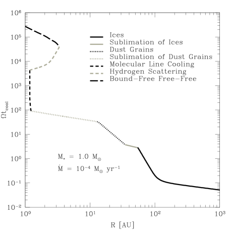
Figure 9: Plot of $\Omega t_{\mathrm{cool}}$ for a mass accretion rate of $10^{-4}\;M_{\odot}\;\mathrm{yr}^{-1}$ indicating the effects of the various opacity regimes.

Fig. 10 also shows how the stability of the disc to fragmentation varies with the background ISM temperature. For low mass accretion rates we see that as the background temperature decreases, the disc actually becomes stable out to larger radii. This can be explained as follows: In the optically thin case where the cooling is dominated by ices (the regime in which this phenomenon is found) the value of $\Omega t_{\mathrm{cool}}$ is given by

$$\Omega t_{\mathrm{cool}} = \frac{3\mathcal{R}\sqrt{2\pi G}}{8\sigma\kappa_{0}}\frac{1}{\mu(\gamma-1)}Q^{1/2}\rho^{1/2}T^{-5}$$ (33)

$$= \frac{3\mathcal{R}\sqrt{GM_{*}}}{8\sigma\kappa_{0}}\frac{1}{\mu(\gamma-1)}R^{-3/2}T^{-5},$$ (34)

where we have used equation 10 to eliminate $\rho$ in equation 34. Hence at a fixed radius $R=R_{\mathrm{frag}}$, increasing the temperature $T$ decreases $\Omega t_{\mathrm{cool}}$ and thereby destabilises the disc. Eventually, for some $T=T_{\mathrm{frag}}$ we reach $\Omega t_{\mathrm{cool}}=15.570$ (from Table 4) and the disc becomes unstable to fragmentation.

From equation 34 we see that on the fragmentation boundary (where by construction $\Omega t_{\mathrm{cool}}=15.570$ is constant), $T_{\mathrm{frag}}\sim R_{\mathrm{frag}}^{-3/10}$. Now assuming that the temperature at which fragmentation occurs is at or above the background temperature (i.e. $T_{\mathrm{frag}}\geq T_{\mathrm{min}}$) then equation 30 holds, and we find similarly that the accretion rate at fragmentation $\dot{M}_{\mathrm{frag}}$ is given by $\dot{M}_{\mathrm{frag}}\sim T_{\mathrm{frag}}^{3/2}$. We therefore find that the radius as which fragmentation occurs increases with decreasing accretion rate such that $R_{\mathrm{frag}}\sim\dot{M}_{\mathrm{frag}}^{-20/9}$. Hence, decreasing the background temperature decreases the accretion rate at which the disc becomes unstable to fragmentation, and likewise increases the radius at which this occurs.

Note however that once $T_{\mathrm{frag}}$ is below the background temperature, (i.e. when $T_{\mathrm{frag}}<T_{\mathrm{min}}$) the disc temperature becomes decoupled from the accretion rate, and hence all accretion rates below $\dot{M}_{\mathrm{min}}=\dot{M}_{\mathrm{frag}}(T_{\mathrm{min}})$ are unstable to fragmentation for radii $R\geq R_{\mathrm{frag}}$.

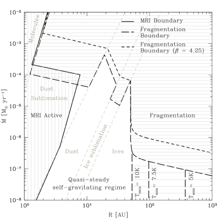
Figure 10: Plot showing the regions expected to be marginally gravitationally stable (unshaded), unstable to fragmentation (horizontal shading) and unstable to the magneto-rotational instability (vertical shading) in a disc about a $1M_{\odot}$ protostar. The cross-hatched regions show where where the disc is unstable to both the MRI and fragmentation. The more widely spaced horizontally shaded region to the lower right would become unstable to fragmentation if the minimum temperature limit of 10K was removed, and the fragmentation boundary moves to the right as the minimum temperature is decreased. The short dashed line corresponds to the fragmentation boundary if a fixed value of $\beta=4.25$ is used (cf. Clarke 2009).

6 Discussion and Conclusions

In summary, we have found from controlled numerical experiments with an imposed temperature dependent cooling law that the effect of temperature dependence is to increase the value of $\Omega t_{\mathrm{cool}}$ at which the disc will fragment into bound objects. Furthermore, this tendency to fragment is greater the more strongly the cooling function depends on the local disc temperature. In this respect, this confirms the results of Johnson & Gammie (2003), who likewise noted a markedly increased tendency towards fragmentation in certain opacity regimes. This result has been attributed to uncertainty in the value of $Q$ in the self-regulated state (Clarke, 2009), equivalent to uncertainty in the equilibrium temperature in our models.

However, our results show that this is only one of two mechanisms that affect the fragmentation boundary, and one that we have been able to account for a posteriori by using effective values of $\beta$ rather than those input to the simulations. The other effect is due to the strength of the intrinsic temperature perturbations about the mean. In the case where the cooling law is dependent on temperature, perturbations about the equilibrium temperature will mean that some fraction of the gas has a lower value of $\Omega t_{\mathrm{cool}}$ than average. Once this fraction reaches a critical value, the disc will become unstable to fragmentation. As the dependence of the cooling on these temperature perturbations increases, at a given average value of $\Omega t_{\mathrm{cool}}$ the percentage of gas that lies below the critical value also increases, and thus the average must increase to avoid fragmentation.

We therefore find that the effect of allowing the cooling function to depend on the local temperature is to make the disc more unstable to fragmentation, and we have been able to quantify this variation (see equation 26). Combining this with predictions of the temperature dependence of protoplanetary discs using opacity-based cooling functions, we find that the fragmentation boundary can be increased by approximately an order of magnitude in terms of $\Omega t_{\mathrm{cool}}$, in close agreement with Johnson & Gammie (2003). We have also found that the RMS strength of the temperature perturbations can be correlated to the average cooling strength (see equation 25), in a very similar manner to that found for the surface density fluctuations (Cossins et al., 2009).

Using these predicted values in analytic models of marginally-gravitationally stable $Q=1$ discs with a representative equation of state, we have found that the susceptibility of such discs to fragmentation into bound objects is also sensitive to the steady state mass accretion rate, as shown in Fig. 10. Others have noted that in the optically thick limit where the opacity is dominated by ices, $\Omega t_{\mathrm{cool}}$ is independent of temperature, and thus the cooling rate is determined only by the local density, itself a function of radius (Matzner & Levin, 2005; Rafikov, 2005; Clarke, 2009). It has therefore been suggested that once the cooling becomes dominated by ices fragmentation beyond some radius on the order of 100 $AU$ becomes inevitable, and indeed we find that with a background ISM temperature of $10K$, fragmentation occurs at $\sim 50AU$ for all accretion rates below $\sim 10^{-5}\;M_{\odot}\;\mathrm{yr}^{-1}$.

However, if this minimum temperature condition is relaxed, we find that the change in cooling due to entering the optically thin regime has the effect of stabilising the disc out to large radii. (The fact that allowing it to become cooler actually stabilises the disc is due to the fact that in this regime $\Omega t_{\mathrm{cool}}$ increases with decreasing temperature, and thus a hot disc has a shorter cooling time than a cold one.) For Class II / Classic T Tauri objects embedded in a cold medium with accretion rates below a few times $10^{-7}\;M_{\odot}\;\mathrm{yr}^{-1}$, it is therefore possible that extended discs well beyond 100 $AU$ may be stable against fragmentation (they may well be stable against gravitational instabilitites altogether), and indeed discs with radii of at least 200 $AU$ have been observed (see for example Eisner et al. 2008). Nonetheless, discs with accretion rates at the higher end of the scale ($\dot{M}\approx 10^{-6}\;M_{\odot}\;\mathrm{yr}^{-1}$, Hartmann 2009) will still be unstable to fragmentation at radii beyond $\sim 50AU$. It should be borne in mind however that in the outer regions of discs where the surface density is low, non-thermal ionisation (from cosmic rays, X-rays etc) can trigger the MRI, and this may provide an alternative mechanism for preventing fragmentation, as shown in Clarke (2009).

Fig. 10 also shows another important result, that for accretion rates between $10^{-8}-10^{-2}\;M_{\odot}\;\mathrm{yr}^{-1}$ discs cannot exist in a non-fragmenting purely self-gravitating state at radii $\lesssim 2-5AU$. In this regime discs are either MRI active ($\dot{M}\lesssim 10^{-4}\;M_{\odot}\;\mathrm{yr}^{-1}$) or unstable to fragmentation ($\dot{M}\gtrsim 10^{-4}\;M_{\odot}\;\mathrm{yr}^{-1}$). We also find that in a narrow band of accretion rates $\sim 10^{-4}\;M_{\odot}\;\mathrm{yr}^{-1}$ it is possible for discs to be both MRI active and unstable to fragmentation, although the exact interaction of these two instabilities is uncertain (see Fromang et al. 2004). It is therefore the case that for steady-state protoplanetary discs the gravitational instability cannot drive accretion directly onto the protostar – either the MRI or the thermal instability must act at low radii, as has been proposed for FU Orionis outbursts (Armitage et al. 2001; Zhu et al. 2009).

Finally, our results agree with the generally accepted view that planet formation through gravitationally-induced fragmentation is unlikely to occur at radii less than 50 - 100 $AU$ (Matzner & Levin, 2005; Rafikov, 2005; Whitworth & Stamatellos, 2006; Clarke, 2009; Rafikov, 2009), although this critical radius varies with both the mass accretion rate and the background ISM temperature. Within this radius the core accretion model remains likely to be the dominant mode of planet formation. Outside this radius however, the fragmentation of spiral arms will produce gaseous planets, a result which matches that of Boley (2009) using a grid-based hydrodynamical model with radiative transfer – fragmentation was noted at $\sim 100AU$ about a $1M_{\odot}$ protostar. This result is further corroborated by Stamatellos & Whitworth (2008) whose radiative transfer SPH code suggested a massive disc about a $0.7M_{\odot}$ protostar would rapidly fragment into planetary mass objects or brown dwarf companions beyond approximately $100AU$. Although the mass accretion rate onto the central object is not stated in either case, we find that these figures are nonetheless in general agreement with our predictions.

References

- Alexander et al. (2008) Alexander R. D., Armitage P. J., Cuadra J., 2008, MNRAS, 389, 1655
- Armitage et al. (2001) Armitage P. J., Livio M., Pringle J. E., 2001, MNRAS, 324, 705
- Bate et al. (1995) Bate M. R., Bonnell I. A., Price N. M., 1995, MNRAS, 277, 362
- Bell & Lin (1994) Bell K. R., Lin D. N. C., 1994, ApJ, 427, 987
- Benz (1990) Benz W., 1990, in Numerical Modelling of Nonlinear Stellar Pulsations Problems and Prospects, edited by J. R. Buchler, 269
- Black & Bodenheimer (1975) Black D. C., Bodenheimer P., 1975, ApJ, 199, 619
- Boley (2009) Boley A. C., 2009, ApJL, 695, L53
- Boss (1997) Boss A. P., 1997, Science, 276, 1836
- Boss (1998) Boss A. P., 1998, ApJ, 503, 923
- Clarke (2009) Clarke C. J., 2009, MNRAS, 396, 1066
- Clarke et al. (2007) Clarke C. J., Harper-Clark E., Lodato G., 2007, MNRAS, 381, 1543
- Cossins et al. (2009) Cossins P., Lodato G., Clarke C. J., 2009, MNRAS, 393, 1157
- D’Alessio et al. (1998) D’Alessio P., Canto J., Calvet N., Lizano S., 1998, ApJ, 500, 411
- Dodson-Robinson & Bodenheimer (2009) Dodson-Robinson S. E., Bodenheimer P., 2009, ApJ, 695, L159
- Durisen et al. (2007) Durisen R. H., Boss A. P., Mayer L., Nelson A. F., Quinn T., Rice W. K. M., 2007, in Protostars and Planets V, 607–622
- Eisner et al. (2008) Eisner J. A., Plambeck R. L., Carpenter J. M., Corder S. A., Qi C., Wilner D., 2008, ApJ, 683, 304
- Forgan et al. (2009) Forgan D., Rice K., Stamatellos D., Whitworth A., 2009, MNRAS, 394, 882
- Fromang et al. (2004) Fromang S., Balbus S. A., Terquem C., De Villiers J.-P., 2004, ApJ, 616, 364
- Gammie (2001) Gammie C. F., 2001, ApJ, 553, 174
- Hartmann (2009) Hartmann L., 2009, Accretion Processes in Star Formation: Second Edition, Cambridge University Press
- Hartmann et al. (1998) Hartmann L., Calvet N., Gullbring E., D’Alessio P., 1998, ApJ, 495, 385
- Johnson & Gammie (2003) Johnson B. M., Gammie C. F., 2003, ApJ, 597, 131
- Kalas et al. (2008) Kalas P., Graham J. R., Chiang E., et al., 2008, Science, 322, 1345
- Kennedy & Kenyon (2008) Kennedy G. M., Kenyon S. J., 2008, ApJ, 673, 502
- King et al. (2007) King A. R., Pringle J. E., Livio M., 2007, MNRAS, 376, 1740
- Klahr (2008) Klahr H., 2008, New Astronomy Review, 52, 78
- Lagrange et al. (2009) Lagrange A.-M., Gratadour D., Chauvin G., et al., 2009, A&A, 493, L21
- Levin & Beloborodov (2003) Levin Y., Beloborodov A. M., 2003, ApJL, 590, L33
- Lissauer (1993) Lissauer J. J., 1993, ARA&A, 31, 129
- Lissauer & Stevenson (2007) Lissauer J. J., Stevenson D. J., 2007, in Protostars and Planets V, edited by B. Reipurth, D. Jewitt, K. Keil, 591–606
- Lodato (2007) Lodato G., 2007, Nuovo Cimento Rivista Serie, 30, 293
- Lodato et al. (2005) Lodato G., Delgado-Donate E., Clarke C. J., 2005, MNRAS, 364, L91
- Lodato & Rice (2004) Lodato G., Rice W. K. M., 2004, MNRAS, 351, 630
- Lodato & Rice (2005) Lodato G., Rice W. K. M., 2005, MNRAS, 358, 1489
- Marcy et al. (2005) Marcy G., Butler R. P., Fischer D., et al., 2005, Progress of Theoretical Physics Supplement, 158, 24
- Marois et al. (2008) Marois C., Macintosh B., Barman T., et al., 2008, Science, 322, 1348
- Matzner & Levin (2005) Matzner C. D., Levin Y., 2005, ApJ, 628, 817
- Monaghan (1992) Monaghan J. J., 1992, ARA&A, 30, 543
- Nayakshin & Cuadra (2005) Nayakshin S., Cuadra J., 2005, A&A, 437, 437
- Nayakshin et al. (2007) Nayakshin S., Cuadra J., Springel V., 2007, MNRAS, 379, 21
- Price & Monaghan (2007) Price D. J., Monaghan J. J., 2007, MNRAS, 374, 1347
- Rafikov (2005) Rafikov R. R., 2005, ApJ, 621, L69
- Rafikov (2007) Rafikov R. R., 2007, ApJ, 662, 642
- Rafikov (2009) Rafikov R. R., 2009, arXiv: 0901.4739
- Rice & Armitage (2009) Rice W. K. M., Armitage P. J., 2009, MNRAS, 396, 2228
- Rice et al. (2003) Rice W. K. M., Armitage P. J., Bate M. R., Bonnell I. A., 2003, MNRAS, 339, 1025
- Rice et al. (2005) Rice W. K. M., Lodato G., Armitage P. J., 2005, MNRAS, 364, L56
- Sano et al. (2004) Sano T., Inutsuka S.-i., Turner N. J., Stone J. M., 2004, ApJ, 605, 321
- Shakura & Sunyaev (1973) Shakura N. I., Sunyaev R. A., 1973, A&A, 24, 337
- Springel & Hernquist (2002) Springel V., Hernquist L., 2002, MNRAS, 333, 649
- Stamatellos et al. (2007a) Stamatellos D., Hubber D. A., Whitworth A. P., 2007a, MNRAS, 382, L30
- Stamatellos & Whitworth (2009a) Stamatellos D., Whitworth A., 2009a, ArXiv e-prints
- Stamatellos & Whitworth (2008) Stamatellos D., Whitworth A. P., 2008, A&A, 480, 879
- Stamatellos & Whitworth (2009b) Stamatellos D., Whitworth A. P., 2009b, MNRAS, 392, 413
- Stamatellos et al. (2007b) Stamatellos D., Whitworth A. P., Bisbas T., Goodwin S., 2007b, A&A, 475, 37
- Toomre (1964) Toomre A., 1964, ApJ, 139, 1217
- Whitworth & Stamatellos (2006) Whitworth A. P., Stamatellos D., 2006, A&A, 458, 817
- Winters et al. (2003) Winters W. F., Balbus S. A., Hawley J. F., 2003, ApJ, 589, 543
- Zhu et al. (2009) Zhu Z., Hartmann L., Gammie C., McKinney J. C., 2009, arXiv: 0906.1595