Performance of Statistical Tests for Single Source Detection using Random Matrix Theory

Abstract

This paper introduces a unified framework for the detection of a single source with a sensor array in the context where the noise variance and the channel between the source and the sensors are unknown at the receiver. The Generalized Maximum Likelihood Test is studied and yields the analysis of the ratio between the maximum eigenvalue of the sampled covariance matrix and its normalized trace. Using recent results from random matrix theory, a practical way to evaluate the threshold and the $p$-value of the test is provided in the asymptotic regime where the number $K$ of sensors and the number $N$ of observations per sensor are large but have the same order of magnitude. The theoretical performance of the test is then analyzed in terms of Receiver Operating Characteristic (ROC) curve. It is in particular proved that both Type I and Type II error probabilities converge to zero exponentially as the dimensions increase at the same rate, and closed-form expressions are provided for the error exponents. These theoretical results rely on a precise description of the large deviations of the largest eigenvalue of spiked random matrix models, and establish that the presented test asymptotically outperforms the popular test based on the condition number of the sampled covariance matrix.

I Introduction

The detection of a source by a sensor array is at the heart of many wireless applications. It is of particular interest in the realm of cognitive radio [1, 2] where a multi-sensor cognitive device (or a collaborative network) needs to discover or sense by itself the surrounding environment. This allows the cognitive device to make relevant choices in terms of information to feed back, bandwidth to occupy or transmission power to use. When the cognitive device is switched on, its prior knowledge (on the noise variance for example) is very limited and can rarely be estimated prior to the reception of data. This unfortunately rules out classical techniques based on energy detection [4, 5, 6] and requires new sophisticated techniques exploiting the space or spectrum dimension.

In our setting, the aim of the multi-sensor cognitive detection phase is to construct and analyze tests associated with the following hypothesis testing problem:

$${\boldsymbol{y}}(n)=\left\{\begin{array}[]{ll}{\boldsymbol{w}}(n)&\textrm{under}\ H_{0}\vspace*{.2cm}\\ \displaystyle{\boldsymbol{h}}\>{s}(n)+{\boldsymbol{w}}(n)&\textrm{under}\ H_{1}\\ \end{array}\right.\qquad\textrm{for}\quad n=0:N-1\ ,$$ (1)

where ${\boldsymbol{y}}(n)=[y_{1}(n),\dots,y_{K}(n)]^{T}$ is the observed $K\times 1$ complex time series, ${\boldsymbol{w}}(n)$ represents a $K\times 1$ complex circular Gaussian white noise process with unknown variance $\sigma^{2}$, and $N$ represents the number of received samples. Vector ${\boldsymbol{h}}\in{\mathbb{C}}^{K\times 1}$ is a deterministic vector and typically represents the propagation channel between the source and the $K$ sensors. Signal $s(n)$ denotes a standard scalar independent and identically distributed (i.i.d.) circular complex Gaussian process with respect to the samples $n=0:N-1$ and stands for the source signal to be detected.

The standard case where the propagation channel and the noise variance are known has been thoroughly studied in the literature in the Single Input Single Output case [4, 5, 6] and Multi-Input Multi-Ouput [7] case. In this simple context, the most natural approach to detect the presence of source $s(n)$ is the well-known Neyman-Pearson (NP) procedure which consists in rejecting the null hypothesis when the observed likelihood ratio lies above a certain threshold [8]. Traditionally, the value of the threshold is set in such a way that the Probability of False Alarm (PFA) is no larger than a predefined level $\alpha\in(0,1)$. Recall that the PFA (resp. the miss probability) of a test is defined as the probability that the receiver decides hypothesis $H_{1}$ (resp. $H_{0}$) when the true hypothesis is $H_{0}$ (resp. $H_{1}$). The NP test is known to be uniformly most powerful i.e., for any level $\alpha\in(0,1)$, the NP test has the minimum achievable miss probability (or equivalently the maximum achievable power) among all tests of level $\alpha$. In this paper, we assume on the opposite that:

• the noise variance $\sigma^{2}$ is unknown,

• vector $\boldsymbol{h}$ is unknown.

In this context, probability density functions of the observations ${\boldsymbol{y}}(n)$ under both $H_{0}$ and $H_{1}$ are unknown, and the classical NP approach can no longer be employed. As a consequence, the construction of relevant tests for (1) together with the analysis fo their perfomances is a crucial issue. The classical approach followed in this paper consists in replacing the unknown parameters by their maximum likelihood estimates. This leads to the so-called Generalized Likelihood Ratio (GLR). The Generalized Likelihood Ratio Test (GLRT), which rejects the null hypothesis for large values of the GLR, easily reduces to the statistics given by the ratio of the largest eigenvalue of the sampled covariance matrix with its normalized trace, cf. [9, 10, 11]. Nearby statistics [12, 13, 14, 15], with good practical properties, have also been developed, but would not yield a different (asymptotic) error exponent analysis.

In this paper, we analyze the performance of the GLRT in the asymptotic regime where the number $K$ of sensors and the number $N$ of observations per sensor are large but have the same order of magnitude. This assumption is relevant in many applications, among which cognitive radio for instance, and casts the problem into a large random matrix framework.

Large random matrix theory has already been applied to signal detection [16] (see also [17]), and recently to hypothesis testing [15, 18, 19]. In this article, the focus is mainly devoted to the study of the largest eigenvalue of the sampled covariance matrix, whose behaviour changes under $H_{0}$ or $H_{1}$. The fluctuations of the largest eigenvalue under $H_{0}$ have been described by Johnstone [20] by means of the celebrated Tracy-Widom distribution, and are used to study the threshold and the $p$-value of the GLRT.

In order to characterize the performance of the test, a natural approach would have been to evaluate the Receiver Operating Characteristic (ROC) curve of the GLRT, that is to plot the power of the test versus a given level of confidence. Unfortunately, the ROC curve does not admit any simple closed-form expression for a finite number of sensors and snapshots. As the miss probability of the GLRT goes exponentially fast to zero, the performance of the GLRT is analyzed via the computation of its error exponent, which caracterizes the speed of decrease to zero. Its computation relies on the study of the large deviations of the largest eigenvalue of ’spiked’ sampled covariance matrix. By ’spiked’ we refer to the case where the eigenvalue converges outside the bulk of the limiting spectral distribution, which precisely happens under hypothesis $H_{1}$. We build upon [21] to establish the large deviation principle, and provide a closed-form expression for the rate function.

We also introduce the error exponent curve, and plot the error exponent of the power of the test versus the error exponent for a given level of confidence. The error exponent curve can be interpreted as an asymptotic version of the ROC curve in a $\log$-$\log$ scale and enables us to establish that the GLRT outperforms another test based on the condition number, and proposed by [22, 23, 24] in the context of cognitive radio.

Notice that the results provided here (determination of the threshold of the GLRT test and the computation of the error exponents) would still hold within the setting of real Gaussian random variables instead of complex ones, with minor modifications.

The paper is organized as follows.

Section II introduces the GLRT. The value of the threshold, which completes the definition of the GLRT, is established in Section II-B. As the latter threshold has no simple closed-form expression and as its practical evaluation is difficult, we introduce in Section II-C an asymptotic framework where it is assumed that both the number of sensors $K$ and the number $N$ of available snapshots go to infinity at the same rate. This assumption is valid for instance in cognitive radio contexts and yields a very simple evaluation of the threshold, which is important in real-time applications.

In Section III, we recall several results of large random matrix theory, among which the asymptotic fluctuations of the largest eigenvalue of a sample covariance matrix, and the limit of the largest eigenvalue of a spiked model.

These results are used in Section IV where an approximate threshold value is derived, which leads to the same PFA as the optimal one in the asymptotic regime. This analysis yields a relevant practical method to approximate the $p$-values associated with the GLRT.

Section V is devoted to the performance analysis of the GLRT. We compute the error exponent of the GLRT, derive its expression in closed-form by establishing a Large Deviation Principle for the test statistic $T_{N}$ , and describe the error exponent curve.

Section VI introduces the test based on the condition number, that is the statistics given by the ratio between the largest eigenvalue and the smallest eigenvalue of the sampled covariance matrix. We provide the error exponent curve associated with this test and prove that the latter is outperformed by the GLRT.

Section VII provides further numerical illustrations and conclusions are drawn in Section VIII.

Mathematical details are provided in the Appendix. In particular, a full rigorous proof of a large deviation principle is provided in Appendix A, while a more informal proof of a nearby large deviation principle, maybe more accessible to the non-specialist, is provided in Appendix B.

Notations

For $i\in\{0,1\}$, ${\mathbb{P}}_{i}({\cal E})$ represents the probability of a given event $\cal E$ under hypothesis $H_{i}$. For any real random variable $T$ and any real number $\gamma$, notation

$$T\>_{{}_{H_{0}}}\!\!\gtrless^{{}^{H_{1}}}\gamma$$

stands for the test function which rejects the null hypothesis when $T>\gamma$. In this case, the probability of false alarm (PFA) of the test is given by ${\mathbb{P}}_{0}(T>\gamma)$, while the power of the test is ${\mathbb{P}}_{1}(T>\gamma)$. Notation $\xrightarrow[H_{i}]{a.s.}$ stands for the almost sure (a.s.) convergence under hypothesis $H_{i}$. For any one-to-one mapping $T:{\cal X}\to{\cal Y}$ where $\cal X$ and $\cal Y$ are two sets, we denote by $T^{-1}$ the inverse of $T$ w.r.t. composition. For any borel set $A\in{\mathbb{R}}$, $x\mapsto{\boldsymbol{1}}_{A}(x)$ denotes the indicator function of set $A$ and $\|{\boldsymbol{x}}\|$ denotes the Euclidian norm of a given vector $\boldsymbol{x}$. If ${\boldsymbol{A}}$ is a given matrix, denote by ${\boldsymbol{A}}^{H}$ its transpose-conjugate. If $F$ is a cumulative distribution function (c.d.f.), we denote by $\bar{F}$ is complementary c.d.f., that is: $\bar{F}=1-F$.

II Generalized Likelihood Ratio Test

In this section, we derive the Generalized Likelihood Ratio Test (section II-A) and compute the associated threshold and $p$-value (section II-B). This exact computation raises some computational issues, which are circumvented by the introduction of a relevant asymptotic framework, well-suited for mathematical analysis (Section II-C).

II-A Derivation of the Test

Denote by $N$ the number of observed samples and recall that:

$${\boldsymbol{y}}(n)=\left\{\begin{array}[]{ll}{\boldsymbol{w}}(n)&\textrm{under}\ H_{0}\vspace*{.2cm}\\ \displaystyle{\boldsymbol{h}}\>{s}(n)+{\boldsymbol{w}}(n)&\textrm{under}\ H_{1}\\ \end{array}\right.,\qquad n=0:N-1\ ,$$

where $({\boldsymbol{w}}(n),0\leq n\leq N-1)$ represents an independent and identically distributed (i.i.d.) process of $K\times 1$ vectors with circular complex Gaussian entries with mean zero and covariance matrix $\sigma^{2}{\bf I}_{K}$, vector ${\boldsymbol{h}}\in{\mathbb{C}}^{K\times 1}$ is deterministic, signal $(s(n),0\leq n\leq N-1)$ denotes a scalar i.i.d. circular complex Gaussian process with zero mean and unit variance. Moreover, $({\boldsymbol{w}}(n),0\leq n\leq N-1)$ and $(s(n),0\leq n\leq N-1)$ are assumed to be independent processes. We stack the observed data into a $K\times N$ matrix ${\bf Y}=[{\boldsymbol{y}}(0),\dots,{\boldsymbol{y}}(N-1)]$. Denote by $\hat{\bf R}$ the sampled covariance matrix:

$$\hat{\bf R}=\frac{1}{N}{\bf Y}{\bf Y}^{H},$$

and respectively, by $p_{0}({\bf Y};\sigma^{2})$ and $p_{1}({\bf Y};{\boldsymbol{h}},\sigma^{2})$ the likelihood functions of the observation matrix ${\bf Y}$ indexed by the unknown parameters ${\boldsymbol{h}}$ and $\sigma^{2}$ under hypotheses $H_{0}$ and $H_{1}$.

As ${\bf Y}$ is a $K\times N$ matrix whose columns are i.i.d. Gaussian vectors with covariance matrix ${\bf\Sigma}$ defined by:

$${\bf\Sigma}=\left\{\begin{array}[]{ll}\sigma^{2}{\bf I}_{K}&\textrm{under}\ H_{0}\\ {\boldsymbol{h}}{\boldsymbol{h}}^{H}+\sigma^{2}{\bf I}_{K}&\textrm{under}\ H_{1}\end{array}\right.\ ,$$ (2)

the likelihood functions write:

$$p_{0}({\bf Y};\sigma^{2}) =(\pi\sigma^{2})^{-NK}\exp\left(-\frac{N}{\sigma^{2}}\mathrm{tr}\>{\hat{\bf R}}\right)\ ,$$ (3)

$$p_{1}({\bf Y};{\boldsymbol{h}},\sigma^{2}) =(\pi^{K}\det({\boldsymbol{h}}{\boldsymbol{h}}^{H}+\sigma^{2}{\bf I}_{K}))^{-N}\exp\left(-N\mathrm{tr}\>(\hat{\bf R}({\boldsymbol{h}}{\boldsymbol{h}}^{H}+\sigma^{2}{\bf I}_{K})^{-1})\right)\ .$$ (4)

In the case where parameters $\boldsymbol{h}$ and $\sigma^{2}$ are available, the celebrated Neyman-Pearson procedure yields a uniformly most powerful test, given by the likelihood ratio statistics $\frac{p_{1}({\bf Y};{\boldsymbol{h}},\sigma^{2})}{p_{0}({\bf Y};\sigma^{2})}$.

However, in the case where $\boldsymbol{h}$ and $\sigma^{2}$ are unknown, which is the problem addressed here, no simple procedure garantees a uniformly most powerful test, and a classical approach consists in computing the GLR:

$$L_{N}=\frac{\sup_{{\boldsymbol{h}},\sigma^{2}}p_{1}({\bf Y};{\boldsymbol{h}},\sigma^{2})}{\sup_{\sigma^{2}}p_{0}({\bf Y};\sigma^{2})}\>.$$ (5)

In the GLRT procedure, one rejects hypothesis $H_{0}$ whenever $L_{N}>\xi_{N}$, where $\xi_{N}$ is a certain threshold which is selected in order that the PFA ${\mathbb{P}}_{0}(L_{N}>\xi_{N})$ does not exceed a given level $\alpha$.

In the following proposition, which follows after straightforward computations from [26] and [9], we derive the closed form expression of the GLR $L_{N}$. Denote by $\lambda_{1}>\lambda_{2}>\dots>\lambda_{K}\geq 0$ the ordered eigenvalues of $\hat{\bf R}$ (all distincts with probability one).

Proposition 1.

Let $T_{N}$ be defined by:

$$T_{N}=\frac{\lambda_{1}}{\frac{1}{K}\>\mathrm{tr}\>\hat{\bf R}}\>,$$ (6)

then, the GLR (cf. Eq. (5)) writes:

$$L_{N}=\frac{C}{\left(T_{N}\right)^{N}\left(1-\frac{T_{N}}{K}\right)^{(K-1)N}}$$

where $C=\left(1-\frac{1}{K}\right)^{(1-K)N}$.

By Proposition 1, $L_{N}=\phi_{N,K}(T_{N})$ where $\phi_{N,K}:x\mapsto Cx^{-N}\left(1-\frac{x}{K}\right)^{N(1-K)}$. The GLRT rejects the null hypothesis when inequality $L_{N}>\xi_{N}$ holds. As $T_{N}\in(1,K)$ with probability one and as $\phi_{N,K}$ is increasing on this interval, the latter inequality is equivalent to $T_{N}>\phi_{N,K}^{-1}(\xi_{N})$. Otherwise stated, the GLRT reduces to the test which rejects the null hypothesis for large values of $T_{N}$:

$$T_{N}\begin{array}[]{c}{\footnotesize H_{1}}\\ {\gtrless}\\ {\footnotesize H_{0}}\end{array}\gamma_{N}$$ (7)

where $\gamma_{N}=\phi_{N,K}^{-1}(\xi_{N})$ is a certain threshold which is such that the PFA does not exceed a given level $\alpha$. In the sequel, we will therefore focus on the test statistics $T_{N}$.

Remark 1.

There exist several variants of the above statistics [12, 13, 14, 15], which merely consist in replacing the normalized trace with a more involved estimate of the noise variance. Although very important from a practical point of view, these variants have no impact on the (asymptotic) error exponent analysis. Therefore, we restrict our analysis to the traditional GLRT for the sake of simplicity.

II-B Exact threshold and $p$-values

In order to complete the construction of the test, we must provide a procedure to set the threshold $\gamma_{N}$. As usual, we propose to define $\gamma_{N}$ as the value which maximizes the power ${\mathbb{P}}_{1}(T_{N}>\gamma_{N})$ of the test (7) while keeping the PFA ${\mathbb{P}}_{0}(T_{N}>\gamma_{N})$ under a desired level $\alpha\in(0,1)$. It is well-known (see for instance [8, 27]) that the latter threshold is obtained by:

$$\gamma_{N}=p_{N}^{-1}(\alpha)$$ (8)

where $p_{N}(t)$ represents the complementary c.d.f. of the statistics $T_{N}$ under the null hypothesis:

$$p_{N}(t)={\mathbb{P}}_{0}(T_{N}>t)\>.$$ (9)

Note that $p_{N}(t)$ is continuous and decreasing from 1 to 0 on $t\in[0,\infty)$, so that the threshold $p_{N}^{-1}(\alpha)$ in (8) is always well defined. When the threshold is fixed to $\gamma_{N}=p_{N}^{-1}(\alpha)$, the GLRT rejects the null hypothesis when $T_{N}>p_{N}^{-1}(\alpha)$ or equivalently, when $p_{N}(T_{N})<\alpha$. It is usually convenient to rewrite the GLRT under the following form:

$$p_{N}(T_{N})\begin{array}[]{c}{\tiny{H_{0}}}\\ {\gtrless}\\ {\tiny H_{1}}\end{array}\alpha\>.$$ (10)

The statistics $p_{N}(T_{N})$ represents the significance probability or $p$-value of the test. The null hypothesis is rejected when the $p$-value $p_{N}(T_{N})$ is below the level $\alpha$. In practice, the computation of the $p$-value associated with one experiment is of prime importance. Indeed, the $p$-value not only allows to accept/reject an hypothesis by (10), but it furthermore reflects how strongly the data contradicts the null hypothesis [8].

In order to evaluate $p$-values, we derive in the sequel the exact expression of the complementary c.d.f. $p_{N}$. The crucial point is that $T_{N}$ is a function of the eigenvalues $\lambda_{1},\dots,\lambda_{K}$ of the sampled covariance matrix $\hat{\bf R}$. We have

$$p_{N}(t)=\int_{\Delta_{t}}p_{K,N}^{0}(x_{1},\cdots,x_{K})\textrm{d}x_{1:K}$$ (11)

where for each $t$, the domain of integration $\Delta_{t}$ is defined by:

$$\Delta_{t}=\left\{(x_{1},\dots,x_{K})\in\mathbb{R}^{K},\ \frac{Kx_{1}}{x_{1}+\dots+x_{K}}>t\right\}\ ,$$

and $p_{K,N}^{0}$ is the joint probability density function (p.d.f.) of the ordered eigenvalues of ${\bf\hat{R}}$ under $H_{0}$ given by:

$$p_{K,N}^{0}(x_{1:K})=\frac{{\boldsymbol{1}}_{(x_{1}\geq\dots\geq x_{K}\geq 0)}}{Z_{K,N}^{0}}\prod_{1\leq i<j\leq K}(x_{j}-x_{i})^{2}\>\prod_{j=1}^{K}x_{j}^{N-K}e^{-Nx_{j}}$$ (12)

where ${\boldsymbol{1}}_{(x_{1}\geq\dots\geq x_{K}\geq 0)}$ stands for the indicator function of the set $\{(x_{1}\dots x_{K})\>:\>x_{1}\geq\dots\geq x_{K}\geq 0\}$ and where $Z_{K,N}^{0}$ is the normalization constant (see for instance [28], [29, Chapter 4]).

Remark 2.

For each $t$, the computation of $p_{N}(t)$ requires the numerical evaluation of a non-trivial integral. Despite the fact that powerful numerical methods, based on representations of such integrals with hypergeometric functions [30], are available (see for instance [31], [32]), an on line computation, requested in a number of real-time applications, may be out of reach.

Instead, tables of the function $p_{N}$ should be computed off line i.e., prior to the experiment. As both the dimensions $K$ and $N$ may be subject to frequent changes, all possible tables of the function $p_{N}$ should be available at the detector’s side, for all possible values of the couple $(N,K)$. This both requires substantial computations and considerable memory space. In what follows, we propose a way to overcome this issue.

In the sequel, we study the asymptotic behaviour of the complementary c.d.f. $p_{N}$ when both the number of sensors $K$ and the number of snapshots $N$ go to infinity at the same rate. This analysis leads to simpler testing procedure.

II-C Asymptotic framework

We propose to analyze the asymptotic behaviour of the complementary c.d.f. $p_{N}$ as the number of observations goes to infinity. More precisely, we consider the case where both the number $K$ of sensors and the number $N$ of snapshots go to infinity at the same speed, as assumed below

$$N\to\infty,\;K\to\infty,\;\;c_{N}:=\frac{K}{N}\to c,\textrm{ with }0<c<1.$$ (13)

This asymptotic regime is relevant in cases where the sensing system must be able to perform source detection in a moderate amount of time i.e., the number $K$ of sensors and the number $N$ of samples being of the same order. This is in particular the case in cognitive radio applications (see for instance [33]). Very often, the number of sensors is lower than the number of snapshots, hence the ratio $c$ lower than 1.

In the sequel, we will simply denote $N,K\to\infty$ to refer to the asymptotic regime (13).

Remark 3.

The results related to the GLRT presented in Sections IV and V remain true for $c\geq 1$; in the case of the test based on the condition number and presented in Section VI, extra-work is needed to handle the fact that the lowest eigenvalue converges to zero, which happens if $c\geq 1$.

III Large random matrices - Largest eigenvalue - Behaviour of the GLR statistics

In this section, we recall a few facts on large random matrices as the dimensions $N,K$ go to infinity. We focus on the behaviour of the eigenvalues of $\bf\hat{R}$ which differs whether hypothesis $H_{0}$ holds (Section III-A) or $H_{1}$ holds (Section III-B).

As the column vectors of ${\bf Y}$ are i.i.d. complex Gaussian with covariance matrix ${\bf\Sigma}$ given by (2), the probability density of ${\bf\hat{R}}$ is given by:

$$\frac{1}{Z(N,K,{\bf\Sigma})}e^{-N\mathrm{tr}({\bf\Sigma}^{-1}{\bf\hat{R}})}(\textrm{det }{\bf\hat{R}})^{N-K},$$

where $Z(N,K,{\bf\Sigma})$ is a normalizing constant.

III-A Behaviour under hypothesis $H_{0}$

As the behaviour of $T_{N}$ does not depend on $\sigma^{2}$, we assume that $\sigma^{2}=1$; in particular, ${\bf\Sigma}={\bf I}_{K}.$ Under $H_{0}$, matrix $\hat{\bf R}$ is a complex Wishart matrix and it is well-known (see for instance [28]) that the Jacobian of the transformation between the entries of the matrix and the eigenvalues/angles is given by the Vandermonde determinant $\prod_{1\leq i<j\leq K}(x_{j}-x_{i})^{2}.$ This yields the joint p.d.f. of the ordered eigenvalues (12) where the normalizing constant $Z(N,K,{\bf I}_{K})$ is denoted by $Z_{K,N}^{0}$ for simplicity.

The celebrated result from Mar$\check{\textrm{c}}$enko and Pastur [34] states that the limit as $N,K\to\infty$ of the c.d.f. $F_{N}(x)=\frac{\#\{i,\,\lambda_{i}\leq x\}}{K}$ associated to the empirical distribution of the eigenvalues ($\lambda_{i}$) of $\hat{\bf R}$ is equal to $\mathbb{P}_{\check{\mathrm{M}}\mathrm{P}}\left((-\infty,x]\right)$ where $\mathbb{P}_{\check{\mathrm{M}}\mathrm{P}}$ represents the Mar$\check{\mathrm{c}}$enko-Pastur distribution:

$$\mathbb{P}_{\check{\mathrm{M}}\mathrm{P}}(dy)=\mathbf{1}_{(\lambda^{-},\lambda^{+})}(y)\frac{\sqrt{(\lambda^{+}-y)(y-\lambda^{-})}}{2\pi cy}\,dy,$$ (14)

with $\lambda^{+}=(1+\sqrt{c})^{2}$ and $\lambda^{-}=(1-\sqrt{c})^{2}$. This convergence is very fast in the sense that the probability of deviating from $\mathbb{P}_{\check{\mathrm{M}}\mathrm{P}}$ decreases as $e^{-N^{2}\times\textrm{const.}}.$ More precisely, a simple application of the large deviations results in [35] yields that for any distance $d$ on the set of probability measures on $\mathbb{R}$ compatible with the weak convergence and for any $\delta>0,$

$$\limsup_{N\to\infty}\frac{1}{N}\log\mathbb{P}_{0}\left(d(F_{N},\mathbb{P}_{\check{\mathrm{M}}\mathrm{P}})>\delta\right)=-\infty\ .$$ (15)

Moreover, the largest eigenvalue $\lambda_{1}$ of $\hat{\bf R}$ converges a.s. to the right edge of the Mar$\check{\mathrm{c}}$enko-Pastur distribution, that is $(1+\sqrt{c})^{2}.$ A further result due to Johnstone [20] describes its speed of convergence ($N^{-2/3}$) and its fluctuations (see also [36] for complementary results). Let $\Lambda_{1}$ be defined by:

$$\Lambda_{1}=N^{2/3}\left(\frac{\lambda_{1}-(1+\sqrt{c_{N}})^{2}}{b_{N}}\right)\ ,$$ (16)

where $b_{N}$ is defined by

$$b_{N}:=(1+\sqrt{c_{N}})\left(\frac{1}{\sqrt{c_{N}}}+1\right)^{1/3}\>,$$ (17)

then $\Lambda_{1}$ converges in distribution toward a standard Tracy-Widom random variable with c.d.f. $F_{TW}$ defined by:

$$F_{TW}(x)=\exp\left(-\int_{x}^{\infty}(u-x)q^{2}(u)\,du\right)\,\quad\forall x\in\mathbb{R}\ ,$$ (18)

where $q$ solves the Painlevé II differential equation:

$$q^{\prime\prime}(x)=xq(x)+2q^{3}(x),\quad q(x)\sim\textrm{Ai}(x)\quad\textrm{as}\quad x\to\infty$$

and where Ai$(x)$ denotes the Airy function. In particular, $F_{TW}$ is continuous. The Tracy-Widom distribution was first introduced in [37, 38] as the asymptotic distribution of the centered and rescaled largest eigenvalue of a matrix from the Gaussian Unitary Ensemble.

Tables of the Tracy-Widom law are available for instance in [39], while a practical algorithm allowing to efficiently evaluate equation (18) can be found in [40].

Remark 4.

In the case where the entries of matrix ${\bf Y}$ are real Gaussian random variables, the fluctuations of the largest eigenvalue are still described by a Tracy-Widom distribution whose definition slightly differs from the one given in the complex case (for details, see [20]).

III-B Behaviour under hypothesis $H_{1}$

In this case, the covariance matrix writes ${\bf\Sigma}=\sigma^{2}{\bf I}_{K}+{\bf h}{\bf h}^{*}$ and matrix ${\bf\hat{R}}$ follows a single spiked model. Since the behaviour of $T_{N}$ is not affected if the entries of ${\bf Y}$ are multiplied by a given constant, we find it convenient to consider the model where ${\bf\Sigma}={\bf I}_{K}+\frac{{\bf h}{\bf h}^{*}}{\sigma^{2}}$. Denote by

$$\rho_{K}=\frac{\|{\bf h}\|^{2}}{\sigma^{2}}$$

the signal-to-noise ratio (SNR), then matrix ${\bf\Sigma}$ admits the decomposition ${\bf\Sigma}={\bf U}{\bf D}{\bf U}^{*}$ where ${\bf U}$ is a unitary matrix and ${\bf D}={\rm diag}\left(\rho_{K},1,\ldots,1\right).$ With the same change of variables from the entries of the matrix to the eigenvalues/angles with Jacobian $\prod_{1\leq i<j\leq K}(x_{j}-x_{i})^{2},$ the p.d.f. of the ordered eigenvalues writes:

$$p_{K}^{1,N}(x_{1:K})=\frac{{\boldsymbol{1}}_{(x_{1}\geq\dots\geq x_{K}\geq 0)}}{Z_{K,N}^{1}}\prod_{1\leq i<j\leq K}(x_{j}-x_{i})^{2}\>\prod_{j=1}^{K}x_{j}^{N-K}e^{-Nx_{j}}I_{K}\left(\frac{N}{K}{\bf B}_{K},{\bf X}_{K}\right)$$ (19)

where the normalizing constant $Z(N,K,{\bf I}_{K}+{\bf hh^{*}})$ is denoted by $Z_{K,N}^{1}$ for simplicity, ${\bf X}_{K}$ is the diagonal matrix with eigenvalues $(x_{1},\dots,x_{K}),$ ${\bf B}_{K}$ is the $K\times K$ diagonal matrix with eigenvalues $(\frac{\rho_{K}}{1+\rho_{K}},0,\dots,0)$, and for any real diagonal matrices ${\bf C}_{K},{\bf D}_{K},$ the spherical integral $I_{K}({\bf C}_{K},{\bf D}_{K})$ is defined as

$$I_{K}({\bf C}_{K},{\bf D}_{K})=\int e^{K\mathrm{tr}({\bf C}_{K}{\bf Q}{\bf D}_{K}{\bf Q}^{H})}dm_{K}({\bf Q}),$$ (20)

with $m_{K}$ the Haar measure on the unitary group of size $K$ (see [30, Chapter 3] for details).

Whereas this rank-one perturbation does not affect the asymptotic behaviour of $F_{N}$ (the convergence toward $\mathbb{P}_{\check{\mathrm{M}}\mathrm{P}}$ and the deviations of the empirical measure given by (15) still hold under $\mathbb{P}_{1}$), the limiting behaviour of the largest eigenvalue $\lambda_{1}$ can change if the signal-to-noise ratio $\rho_{K}$ is large enough.

Assumption 1.

The following constant $\rho\in{\mathbb{R}}$ exists:

$$\rho=\lim_{K\to\infty}\frac{\|{\boldsymbol{h}}\|^{2}}{\sigma^{2}}\ \left(=\lim_{K\to\infty}\rho_{K}\right)\>.$$ (21)

We refer to $\rho$ as the limiting SNR. We also introduce

$$\lambda_{\mathrm{spk}}^{\infty}=(1+\rho)\left(1+\frac{c}{\rho}\right).$$

Under hypothesis $H_{1}$, the largest eigenvalue has the following asymptotic behaviour as $N,K$ go to infinity:

$$\lambda_{1}\xrightarrow[H_{1}]{a.s.}\left\{\begin{array}[h]{ll}\lambda_{\mathrm{spk}}^{\infty}&\textrm{if }\rho>\sqrt{c}\>,\vspace*{.2cm}\\ \lambda^{+}&\textrm{otherwise,}\end{array}\right.$$ (24)

see for instance [41] for a proof of this result. Note in particular that $\lambda_{\mathrm{spk}}^{\infty}$ is strictly larger than the right edge of the support $\lambda^{+}$ whenever $\rho>\sqrt{c}$. Otherwise stated, if the perturbation is large enough, the largest eigenvalue converges outside the support of Mar$\check{\mathrm{c}}$enko-Pastur distribution.

III-C Limiting behaviour of $T_{N}$ under $H_{0}$ and $H_{1}$

Gathering the results recalled in Sections III-A and III-B, we obtain the following:

Proposition 2.

Let Assumption 1 hold true and assume that $\rho>\sqrt{c}$, then:

$$T_{N}\xrightarrow[H_{0}]{a.s.}(1+\sqrt{c})^{2}\quad\textrm{and}\quad T_{N}\xrightarrow[H_{1}]{a.s.}(1+\rho)\left(1+\frac{c}{\rho}\right)\quad\textrm{as}\ N,K\rightarrow\infty.$$

IV Asymptotic threshold and $p$-values

IV-A Computation of the asymptotic threshold and $p$-value

In Theorem 1 below, we take advantage of the convergence results of the largest eigenvalue of $\hat{\bf R}$ under $H_{0}$ in the asymptotic regime $N,K\to\infty$ to express the threshold and the $p$-value of interest in terms of Tracy-Widom quantiles. Recall that $\bar{F}_{TW}=1-F_{TW}$, that $c_{N}=\frac{K}{N}$, and that $b_{N}$ is given by (17).

Theorem 1.

Consider a fixed level $\alpha\in(0,1)$ and let $\gamma_{N}$ be the threshold for which the power of test (7) is maximum, i.e. $p_{N}(\gamma_{N})=\alpha$ where $p_{N}$ is defined by (11). Then:

1. The following convergence holds true:

   $$\zeta_{N}\ \stackrel{{\scriptstyle\triangle}}{{=}}\ \frac{N^{2/3}}{b_{N}}\left(\gamma_{N}-(1+\sqrt{c_{N}})^{2}\right)\ \xrightarrow[N,K\rightarrow\infty]{}\ \bar{F}_{TW}^{-1}(\alpha)\ .$$

2. The PFA of the following test

   $$T_{N}\begin{array}[]{c}{\footnotesize H_{1}}\\ {\gtrless}\\ {\footnotesize H_{0}}\end{array}(1+\sqrt{c_{N}})^{2}+\frac{b_{N}}{N^{2/3}}\>\bar{F}_{TW}^{-1}(\alpha)$$ (25)

   converges to $\alpha$.

3. The $p$-value $p_{N}(T_{N})$ associated with the GLRT can be approximated by:

   $$\tilde{p}_{N}(T_{N})=\bar{F}_{TW}\left(\frac{N^{2/3}(T_{N}-(1+\sqrt{c_{N}})^{2})}{b_{N}}\right)$$ (26)

   in the sense that $p_{N}(T_{N})-\tilde{p}_{N}(T_{N})\to 0$.

Remark 5.

Theorem 1 provides a simple approach to compute both the threshold and the $p$-values of the GLRT as the dimension $K$ of the observed time series and the number $N$ of snapshots are large: The threshold $\gamma_{N}$ associated with the level $\alpha$ can be approximated by the righthand side of (25). Similarly, equation (26) provides a convenient approximation for the $p$-value associated with one experiment. These approaches do not require the tedious computation of the exact complementary c.d.f. (11) and, instead, only rely on tables of the c.d.f. $F_{TW}$, which can be found for instance in [39] along with more details on the computational aspects (note that function $F_{TW}$ does not depend on any of the problem’s characteristic, and in particular not on $c$). This is of importance in real-time applications, such as cognitive radio for instance, where the users connected to the network must quickly decide for the presence/absence of a source.

Proof of Theorem 1.

Before proving the three points of the theorem, we first describe the fluctuations of $T_{N}$ under $H_{0}$ with the help of the results in Section III-A. Assume without loss of generality that $\sigma^{2}=1$, recall that $T_{N}=\frac{\lambda_{1}}{K^{-1}\mathrm{tr}\hat{\bf R}}$ and denote by:

$$\tilde{T}_{N}=\frac{N^{2/3}(T_{N}-(1+\sqrt{c_{N}})^{2})}{b_{N}}$$ (27)

the rescaled and centered version of the statistics $T_{N}$. A direct application of Slutsky’s lemma (see for instance [42]) together with the fluctuations of $\lambda_{1}$ as reminded in Section III-A yields that $\tilde{T}_{N}$ converges in distribution to a standard Tracy-Widom random variable with c.d.f. $F_{TW}$ which is continuous over $\mathbb{R}$. Denote by $F_{N}$ the c.d.f. of $\tilde{T}_{N}$ under $H_{0}$, then a classical result, sometimes called Polya’s theorem (see for instance [43]), asserts that the convergence of $F_{N}$ towards $F_{TW}$ is uniform over $\mathbb{R}$:

$$\sup_{x\in\mathbb{R}}|F_{N}(x)-F_{TW}(x)|\xrightarrow[N,K\to\infty]{}0\ .$$ (28)

We are now in position to prove the theorem.

The mere definition of $\zeta_{N}$ implies that $\alpha=p_{N}(\gamma_{N})={\bar{F}}_{N}(\zeta_{N})$. Due to (28), $\bar{F}_{TW}(\zeta_{N})\to\alpha$. As $F_{TW}$ has a continuous inverse, the first point of the theorem is proved.

The second point is a direct consequence of the convergence of $F_{N}$ toward the Tracy-Widom distribution: The PFA of test (25) can be written as: ${\mathbb{P}}_{0}\left(\tilde{T}_{N}>\bar{F}_{TW}^{-1}(\alpha)\right)$ which readily converges to $\alpha$.

The third point is a direct consequence of (28): $p_{N}(T_{N})-\tilde{p}_{N}(T_{N})=\bar{F}_{N}(\tilde{T}_{N})-\bar{F}_{TW}(\tilde{T}_{N})\to 0\ .$ This completes the proof of Theorem 1.

∎

V Asymptotic analysis of the power of the test

In this section, we provide an asymptotic analysis of the power of the GLRT as $N,K\to\infty$. As the power of the test goes exponentially to zero, its error exponent is computed with the help of the large deviations associated to the largest eigenvalue of matrix $\hat{\bf R}$. The error exponent and error exponent curve are computed in Theorem 2, Section V-A; the large deviations of interest are stated in Section V-B. Finally Theorem 2 is proved in Section V-C.

V-A Error exponents and error exponent curve

The most natural approach to characterize the performance of a test is to evaluate its power or equivalently its miss probability i.e., the probability under $H_{1}$ that the receiver decides hypothesis $H_{0}$. For a given level $\alpha\in(0,1)$, the miss probability writes:

$$\beta_{N,T}(\alpha)=\inf_{\gamma}\left\{\mathbb{P}_{1}\left(T_{N}<\gamma\right),\ \gamma\ \textrm{such that}\ \mathbb{P}_{0}\left(T_{N}>\gamma\right)\leq\alpha\right\}\ .$$ (29)

Based on Section II-B, the infimum is achieved when the threshold coincides with $\gamma=p_{N}^{-1}(\alpha)$; otherwise stated, $\beta_{N,T}(\alpha)=\mathbb{P}_{1}\left(T_{N}<p_{N}^{-1}(\alpha)\right)$ (notice that the miss probability depends on the unknown parameters $\boldsymbol{h}$ and $\sigma^{2}$). As $\beta_{N,T}(\alpha)$ has no simple expression in the general case, we again study its asymptotic behaviour in the asymptotic regime of interest (13). It follows from Theorem 1 that $p_{N}^{-1}(\alpha)\to\lambda^{+}=(1+\sqrt{c})^{2}$ for $\alpha\in(0,1)$. On the other hand, under hypothesis $H_{1},$ $T_{N}$ converges a.s. to $\lambda_{\mathrm{spk}}^{\infty}$ which is strictly greater than $\lambda^{+}$ when the ratio $\frac{\|{\bf h}\|^{2}}{\sigma^{2}}$ is large enough. In this case, $\mathbb{P}_{1}\left(T_{N}<p_{N}^{-1}(\alpha)\right)$ goes to zero as it expresses the probability that $T_{N}$ deviates from its limit $\lambda_{\mathrm{spk}}^{\infty}$; moreover, one can prove that the convergence to zero is exponential in $N$:

$$\mathbb{P}_{1}\left(T_{N}<x\right)\propto e^{-NI_{\rho}^{+}(x)}\qquad\textrm{for}\quad x\leq\lambda_{\mathrm{spk}}^{\infty}\ ,$$ (30)

where $I_{\rho}^{+}$ is the so-called rate function associated to $T_{N}$. This observation naturally yields the following definition of the error exponent ${\mathcal{E}}_{T}$:

$${\cal E}_{T} = \lim_{N,K\to\infty}-\frac{1}{N}\log\beta_{N,T}(\alpha)$$ (31)

the existence of which is established in Theorem 2 below (as $N,K\to\infty$). Also proved is the fact that ${\mathcal{E}}_{T}$ does not depend on $\alpha$.

The error exponent ${\cal E}_{T}$ gives crucial information on the performance of the test $T_{N}$, provided that the level $\alpha$ is kept fixed when $N,K$ go to infinity. Its existence strongly relies on the study of the large deviations associated to the statistics $T_{N}$.

In practice however, one may as well take benefit from the increasing number of data not only to decrease the miss probability, but to decrease the PFA as well. As a consequence, it is of practical interest to analyze the detection performance when both the miss probability and the PFA go to zero at exponential speed. A couple $(a,b)\in(0,\infty)\times(0,\infty)$ is said to be an achievable pair of error exponents for the test $T_{N}$ if there exists a sequence of levels $\alpha_{N}$ such that, in the asymptotic regime (13),

$$\lim_{N,K\to\infty}-\frac{1}{N}\log\alpha_{N}=a\quad\textrm{and}\quad\lim_{N,K\to\infty}-\frac{1}{N}\log\beta_{N,T}(\alpha_{N})=b\ .$$ (32)

We denote by ${\cal S}_{T}$ the set of achievable pairs of error exponents for test $T_{N}$ as $N,K\to\infty$. We refer to ${\cal S}_{T}$ as the error exponent curve of $T_{N}$.

The following notations are needed in order to describe the error exponent ${\mathcal{E}}_{T}$ and error exponent curve ${\cal S}_{T}$.

$$\left\{\begin{array}[]{lcll}\mathbf{f}(x)&=&\int\frac{1}{y-x}\mathbb{P}_{\check{\mathrm{M}}\mathrm{P}}(dy)&\textrm{for}\ x\in\mathbb{R}\setminus(\lambda^{-},\lambda^{+})\\ \mathbf{F}^{+}(x)&=&\int\log(x-y)\mathbb{P}_{\check{\mathrm{M}}\mathrm{P}}(dy)&\textrm{for}\ x\geq\lambda^{+}\end{array}\right.\ .$$ (33)

Remark 6.

Function $\mathbf{f}$ is the well-known Stieltjes transform associated to Mar$\check{\mathrm{c}}$enko-Pastur distribution and admits a closed-form representation formula. So does function $\mathbf{F}^{+}$, although this fact is perhaps less known. These results are gathered in Appendix C.

Denote by $\Delta(\,\cdot\mid A)$ the convex indicator function i.e. the function equal to zero for $x\in A$ and to infinity otherwise. For $\rho>\sqrt{c}$, define the function:

$$I^{+}_{\rho}(x) = \frac{x-\lambda_{\mathrm{spk}}^{\infty}}{(1+\rho)}-\left(1-c\right)\log\left(\frac{x}{\lambda_{\mathrm{spk}}^{\infty}}\right)-c\left(\mathbf{F}^{+}(x)-\mathbf{F}^{+}(\lambda_{\mathrm{spk}}^{\infty})\right)+\Delta(x\mid[\lambda^{+},\infty))\ .$$ (34)

Also define the function:

$$I^{+}_{0}(x)=x-\lambda^{+}-\left(1-c\right)\log\left(\frac{x}{\lambda^{+}}\right)-2c\left(\mathbf{F}^{+}(x)-\mathbf{F}^{+}(\lambda^{+})\right)+\Delta(x\mid[\lambda^{+},\infty))\ .$$ (35)

We are now in position to state the main theorem of the section:

Theorem 2.

Let Assumption 1 hold true, then:

1. For any fixed level $\alpha\in(0,1)$, the limit ${\cal E}_{T}$ in (31) exists as $N,K\to\infty$ and satisfies:

   $${\mathcal{E}}_{T}=I^{+}_{\rho}(\lambda^{+})$$ (36)

   if $\rho>\sqrt{c}$ and ${\mathcal{E}}_{T}=0$ otherwise.

2. The error exponent curve of test $T_{N}$ is given by:

   $${\cal S}_{T} = \left\{(I_{0}^{+}(x),I_{\rho}^{+}(x))\>:\>x\in(\lambda^{+},\lambda_{\mathrm{spk}}^{\infty})\right\}$$ (37)

   if $\rho>\sqrt{c}$ and ${\cal S}_{T}=\emptyset$ otherwise.

The proof of Theorem 2 heavily relies on the large deviations of $T_{N}$ and is postponed to Section V-C. Before providing the proof, it is worth making the following remarks.

Remark 7.

Several variants of the GLRT have been proposed in the literature, and typically consist in replacing the denominator $\frac{1}{K}\mathrm{tr}\,{\hat{\bf R}}$ (which converges toward $\sigma^{2}$) by a more involved estimate of $\sigma^{2}$ in order to decrease the bias [12, 13, 14, 15]. However, it can be established that the error exponents of the above variants are as well given by (36) and (37) in the asymptotic regime.

Remark 8.

The error exponent ${\mathcal{E}}_{T}$ yields a simple approximation of the miss probability in the sense that $\beta_{N,T}(\alpha)\simeq e^{-N\,{\mathcal{E}}_{T}}$ as $N\to\infty$. It depends on the limiting ratio $c$ and on the value of the SNR $\rho$ through the constant $\lambda_{\mathrm{spk}}^{\infty}$. In the high SNR case, the error exponent turns out to have a simple expression as a function of $\rho$. If $\rho\to\infty$ then $\lambda_{\mathrm{spk}}^{\infty}$ tends to infinity as well, which simplifies the expression of rate function $I^{+}_{\rho}$. Using ${\bf F}^{+}(\lambda_{\mathrm{spk}}^{\infty})=\log\lambda_{\mathrm{spk}}^{\infty}+o_{\rho}(1)$ where $o_{\rho}(1)$ stands for a term which converges to zero as $\rho\to\infty$, it is straightforward to show that for each $x\geq\lambda^{+}$, $I^{+}_{\rho}(x)=\log\rho-1-(1-c)\log x-c{\bf F}^{+}(x)+o_{\rho}(1)$. After some algebra, we finally obtain:

$${\mathcal{E}}_{T}=\log\rho-(1+\sqrt{c})-(1-c)\log(1+\sqrt{c})-c\log\sqrt{c}+o_{\rho}(1)\ .$$

At high SNR, this yields the following convenient approximation of the miss probability:

$$\beta_{N,T}(\alpha)\simeq\left(\psi(c)\,\rho\right)^{N}\ ,$$ (38)

where $\psi(c)=e^{-(1+\sqrt{c})}(1+\sqrt{c})^{c-1}{c}^{-\frac{c}{2}}$.

V-B Large Deviations associated to $T_{N}$

In order to express the error exponents of interest, a rigorous formalization of (30) is needed. Let us recall the definition of a Large Deviation Principle: A sequence of random variables $(X_{N})_{N\in\mathbb{N}}$ satisfies a Large Deviation Principle (LDP) under $\mathbb{P}$ in the scale $N$ with good rate function $I$ if the following properties hold true:

• $I$ is a nonnegative function with compact level sets, i.e. $\{x,I(x)\leq t\}$ is compact for $t\in\mathbb{R},$

• for any closed set $F\subset\mathbb{R},$ the following upper bound holds true:

  $$\limsup_{N\to\infty}\frac{1}{N}\log\mathbb{P}(X_{N}\in F)\leq-\inf_{F}I\ .$$ (39)

• for any open set $G\subset\mathbb{R},$ the following lower bound holds true:

  $$\liminf_{N\to\infty}\frac{1}{N}\log\mathbb{P}(X_{N}\in G)\geq-\inf_{G}I\ .$$ (40)

For instance, if $A$ is a set such that $\inf_{\textrm{int}(A)}I=\inf_{\textrm{cl}(A)}I(=\inf_{A}I)$, (where $\textrm{int}(A)$ and $\textrm{cl}(A)$ respectively denote the interior and the closure of $A$), then (39) and (40) yield

$$\lim_{N\to\infty}N^{-1}\log\mathbb{P}(X_{N}\in A)=-\inf_{A}I\ .$$ (41)

Informally stated,

$$\mathbb{P}(X_{N}\in A)\quad\propto\quad e^{-N\inf_{A}I}\qquad\textrm{as}\ N\to\infty\ .$$

If, moreover $\inf_{A}I>0$ (which typically happens if the limit of $X_{N}$ -if existing- does not belong to $A$), then probability $\mathbb{P}(X_{N}\in A)$ goes to zero exponentially fast, hence a large deviation (LD); and the event $\{X_{N}\in A\}$ can be referred to as a rare event. We refer the reader to [44] for further details on the subject.

As already mentioned above, all the probabilities of interest are rare events as $N,K$ go to infinity related to large deviations for $T_{N}.$ More precisely, Theorem 2 is merely a consequence of the following Lemma.

Lemma 1.

Let Assumption 1 hold true and let $N,K\to\infty$, then:

1. Under $H_{0},$ $T_{N}$ satisfies the LDP in the scale $N$ with good rate function $I_{0}^{+}$, which is increasing from 0 to $\infty$ on interval $[\lambda^{+},\infty)$.

2. Under $H_{1}$ and if $\rho>\sqrt{c}$, $T_{N}$ satisfies the LDP in the scale $N$ with good rate function $I_{\rho}^{+}.$ Function $I_{\rho}^{+}$ is decreasing from $I_{\rho}^{+}(\lambda^{+})$ to 0 on $[\lambda^{+},\lambda_{\mathrm{spk}}^{\infty}]$ and increasing from 0 to $\infty$ on $[\lambda_{\mathrm{spk}}^{\infty},\infty)$.

3. For any bounded sequence $(\eta_{N})_{N\geq 0}$,

   $$\lim_{N,K\to\infty}-\frac{1}{N}\log{\mathbb{P}}_{1}\left(T_{N}<(1+\sqrt{c_{N}})^{2}+\frac{\eta_{N}}{N^{2/3}}\right)=\left\{\begin{array}[h]{ll}I_{\rho}^{+}(\lambda^{+})&\textrm{ if }\rho>\sqrt{c}\\ 0&\textrm{otherwise.}\end{array}\right.$$ (42)

4. Let $x\in(\lambda^{+},\infty)$ and let $(x_{N})_{N\geq 0}$ be any real sequence which converges to $x$. If $\rho\leq\sqrt{c}$, then:

   $$\lim_{N,K\to\infty}-\frac{1}{N}\log{\mathbb{P}}_{1}\left(T_{N}<x_{N}\right)=0\ .$$ (43)

The proof of Lemma 1 is provided in Appendix A.

Remark 9.

1. The proof of the large deviations for $T_{N}$ relies on the fact that the denominator $K^{-1}\mathrm{tr}\,\hat{\bf R}$ of $T_{N}$ concentrates much faster than $\lambda_{1}$. Therefore, the large deviations of $T_{N}$ are driven by those of $\lambda_{1}$, a fact that is exploited in the proof.

2. In Appendix A, we rather focus on the large deviations of $\lambda_{1}$ under $H_{1}$ and skip the proof of Lemma 1-(1), which is simpler and available (to some extent) in [29, Theorem 2.6.6]. Indeed, the proof of the LDP relies on the joint density of the eigenvalues. Under $H_{1}$, this joint density has an extra-term, the spherical integral, and is thus harder to analyze.

3. Lemma 1-(3) is not a mere consequence of Lemma 1-(2) as it describes the deviations of $T_{N}$ at the vicinity of a point of discontinuity of the rate function. The direct application of the LDP would provide a trivial lower bound ($-\infty$) in this case.

4. In the case where the entries of matrix ${\bf Y}$ are real Gaussian random variables, the results stated in Lemma 1 will still hold true with minor modifications: The rate functions will be slightly different. Indeed, the computation of the rate functions relies on the joint density of the eigenvalues, which differs whether the entries of ${\bf Y}$ are real or complex.

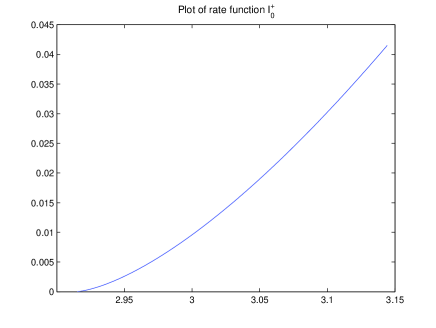
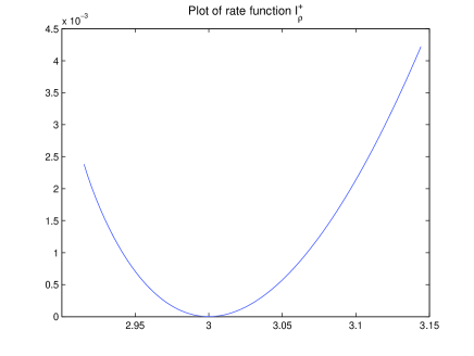
Figure 1: Plots of rate functions $I_{0}^{+}$ and $I_{\rho}^{+}$ in the case where $c=0.5$ and $\rho=1\,db$. In this case, $\lambda^{+}=2.9142$, $\lambda_{\mathrm{spk}}^{\infty}=3$, $I_{0}^{+}(\lambda^{+})=0$ and $I_{\rho}^{+}(\lambda_{\mathrm{spk}}^{\infty})=0$.

V-C Proof of Theorem 2

In order to prove (36), we must study the asymptotic behaviour of the miss probability $\beta_{N,T}(\alpha)=\mathbb{P}_{1}\left(T_{N}<p_{N}^{-1}(\alpha)\right)$ as $N,K\to\infty$. Using Theorem 1-(1), we recall that

$$\beta_{N,T}(\alpha)=\mathbb{P}_{1}\left(T_{N}<(1+\sqrt{c_{N}})^{2}+\frac{\eta_{N}}{N^{2/3}}\right)$$ (44)

where $c_{N}=\frac{K}{N}$ converges to $c$ and where $\eta_{N}$ is a deterministic sequence such that

$$\lim_{N,K\to\infty}\eta_{N}=(1+\sqrt{c})\left(\frac{1}{\sqrt{c}}+1\right)^{1/3}\bar{F}_{TW}^{-1}(\alpha)\>.$$

Hence, Lemma 1-(3) yields the first point of Theorem 2. We now prove the second point. Assume that $\rho>\sqrt{c}$. Consider any $x\in(\lambda^{+},\lambda_{\mathrm{spk}}^{\infty})$ and for every $N,K$, consider the test function which rejects the null hypothesis when $T_{N}>x,$

$$T_{N}\begin{array}[]{c}{\footnotesize H_{1}}\\ {\gtrless}\\ {\footnotesize H_{0}}\end{array}x\ .$$ (45)

Denote by $\alpha_{N}={\mathbb{P}}_{0}(T_{N}>x)$ the PFA associated with this test. By Lemma 1-(1) together with the continuity of the rate function at $x$, we obtain:

$$\lim_{N,K\to\infty}-\frac{1}{N}\log\alpha_{N}=\inf_{y\in[x,\infty)}I_{0}^{+}(y)=I_{0}^{+}(x)\ .$$ (46)

The miss probability of this test is given by $\beta_{N,T}(\alpha_{N})={\mathbb{P}}_{1}(T_{N}<x)$. By Lemma 1-(2),

$$\lim_{N,K\to\infty}-\frac{1}{N}\log\beta_{N,T}(\alpha_{N})=\inf_{y\in(-\infty,x]}I_{\rho}^{+}(y)=I_{\rho}^{+}(x)\ .$$ (47)

Equations (46) and (47) prove that $(I_{0}^{+}(x),I_{\rho}^{+}(x))$ is an achievable pair of error exponents. Therefore, the set in the righthand side of (37) is included in ${\cal S}_{T}$. We now prove the converse. Assume that $(a,b)$ is an achievable pair of error exponents and let $\alpha_{N}$ be a sequence such that (32) holds. Denote by $\gamma_{N}=p_{N}^{-1}(\alpha_{N})$ the threshold associated with level $\alpha_{N}$. As $I_{0}^{+}(x)$ is continuous and increasing from 0 to $\infty$ on interval $(\lambda^{+},\infty)$, there exists a (unique) $x\in(\lambda^{+},\infty)$ such that $a=I_{0}^{+}(x)$. We now prove that $\gamma_{N}$ converges to $x$ as $N$ tends to infinity. Consider a subsequence $\gamma_{\varphi(N)}$ which converges to a limit $\gamma\in{\mathbb{R}}\cup\{\infty\}$. Assume that $\gamma>x$. Then there exists $\epsilon>0$ such that $\gamma_{\varphi(N)}>x+\epsilon$ for large $N$. This yields:

$$-\frac{1}{\varphi(N)}\log{\mathbb{P}}_{0}\left(T_{\varphi(N)}>\gamma_{\varphi(N)}\right)\geq-\frac{1}{\varphi(N)}\log{\mathbb{P}}_{0}\left(T_{\varphi(N)}>x+\epsilon\right)\ .$$ (48)

Taking the limit in both terms yields $I_{0}^{+}(x)\geq I_{0}^{+}(x+\epsilon)$ by Lemma 1, which contradicts the fact that $I_{0}^{+}$ is an increasing function. Now assume that $\gamma<x$. Similarly,

$$-\frac{1}{\varphi(N)}\log{\mathbb{P}}_{0}\left(T_{\varphi(N)}>\gamma_{\varphi(N)}\right)\leq-\frac{1}{\varphi(N)}\log{\mathbb{P}}_{0}\left(T_{\varphi(N)}>x-\epsilon\right)$$ (49)

for a certain $\epsilon$ and for $N$ large enough. Taking the limit of both terms, we obtain $I_{0}^{+}(x)\leq I_{0}^{+}(x-\epsilon)$ which leads to the same contradiction. This proves that $\lim_{N}\gamma_{N}=x$. Recall that by definition (32),

$$b=\lim_{N,K\to\infty}-\frac{1}{N}\log{\mathbb{P}}_{1}\left(T_{N}<\gamma_{N}\right)\ .$$

As $\gamma_{N}$ tends to $x$, Lemma 1 implies that the righthand side of the above equation is equal to $I_{\rho}^{+}(x)>0$ if $x\in(\lambda^{+},\lambda_{\mathrm{spk}}^{\infty})$ and $\rho>\sqrt{c}$. It is equal to 0 if $x\geq\lambda_{\mathrm{spk}}^{\infty}$ or $\rho\leq\sqrt{c}$. Now $b>0$ by definition, therefore both conditions $x\in(\lambda^{+},\lambda_{\mathrm{spk}}^{\infty})$ and $\rho>\sqrt{c}$ hold. As a conclusion, if $(a,b)$ is an achievable pair of error exponents, then $(a,b)=(I_{0}^{+}(x),I_{\rho}^{+}(x))$ for a certain $x\in(\lambda^{+},\lambda_{\mathrm{spk}}^{\infty})$, and furthermore $\rho>\sqrt{c}$. This completes the proof of the second point of Theorem 2.

VI Comparison with the test based on the condition number

This section is devoted to the study of the asymptotic performances of the test $U_{N}=\frac{\lambda_{1}}{\lambda_{K}}$, which is popular in cognitive radio [22, 23, 24]. The main result of the section is Theorem 3, where it is proved that the test based on $T_{N}$ asymptotically outperforms the one based on $U_{N}$ in terms of error exponent curves.

VI-A Description of the test

A different approach which has been introduced in several papers devoted to cognitive radio contexts consists in rejecting the null hypothesis for large values of the statistics $U_{N}$ defined by:

$$U_{N}=\frac{\lambda_{1}}{\lambda_{K}}\>,$$ (50)

which is the ratio between the largest and the smallest eigenvalues of $\hat{\bf R}.$ Random variable $U_{N}$ is the so-called condition number of the sampled covariance matrix $\hat{\bf R}$. As for $T_{N}$, an important feature of the statistics $U_{N}$ is that its law does not depend of the unknown parameter $\sigma$ which is the level of the noise. Under hypothesis $H_{0}$, recall that the spectral measure of $\hat{\bf R}$ weakly converges to the Mar$\check{\mathrm{c}}$enko-Pastur distribution (14) with support $(\lambda^{-},\lambda^{+})$. In addition to the fact that $\lambda_{1}$ converges toward $\lambda^{+}$ under $H_{0}$ and $\lambda_{\mathrm{spk}}^{\infty}$ under $H_{1}$, the following result related to the convergence of the lowest eigenvalue is of importance (see for instance [45, 46], [41]):

$$\lambda_{K}\xrightarrow[]{a.s.}\lambda^{-}=\sigma^{2}(1-\sqrt{c})^{2}\$$ (51)

under both hypotheses $H_{0}$ and $H_{1}$. Therefore, the statistics $U_{N}$ admits the following limits:

$$U_{N}\xrightarrow[H_{0}]{a.s.}\frac{\lambda^{+}}{\lambda^{-}}=\frac{(1+\sqrt{c})^{2}}{(1-\sqrt{c})^{2}},\quad\textrm{and}\quad U_{N}\xrightarrow[H_{1}]{a.s.}\frac{\lambda_{\mathrm{spk}}^{\infty}}{\lambda^{-}}\quad\textrm{for}\ \rho>\sqrt{c}\ .$$ (52)

The test is based on the observation that the limit of $U_{N}$ under the alternative $H_{1}$ is strictly larger than the ratio $\lambda^{+}/\lambda^{-}$, at least when the SNR $\rho$ is large enough.

VI-B A few remarks related to the determination of the threshold for the test $U_{N}$

The determination of the threshold for the test $U_{N}$ relies on the asymptotic independence of $\lambda_{1}$ and $\lambda_{K}$ under $H_{0}$. As we shall prove below that test $U_{N}$ is asymptotically outperformed by test $T_{N}$, such a study, rather involved, seems beyond the scope of this article. For the sake of completeness however, we describe unformally how to set the threshold for $U_{N}$. Recall the definition of $\Lambda_{1}$ in (16) and let $\Lambda_{K}$ be defined as:

$$\Lambda_{K}=N^{2/3}\frac{\left(\lambda_{K}-(1-\sqrt{c_{N}})^{2}\right)}{\left(\sqrt{c_{N}}-1\right)\left(c_{N}^{-1/2}-1\right)^{1/3}}\ .$$

Then both $\Lambda_{1}$ and $\Lambda_{K}$ converge toward Tracy-Widom random variables. Moreover,

$$(\Lambda_{1},\Lambda_{K})\xrightarrow[N,K\rightarrow\infty]{}(X,Y)\ ,$$

where $X$ and $Y$ are independent random variables, both distributed according to $F_{TW}$.

As a corollary of the previous convergence, a direct application of the Delta method [27, Chapter 3] yields the following convergence in distribution:

$$N^{2/3}\left(\frac{\lambda_{1}}{\lambda_{K}}-\frac{(1+\sqrt{c_{N}})^{2}}{(1-\sqrt{c_{N}})^{2}}\right)\rightarrow(aX+bY)\ ,$$

where

$$a=\frac{(1+\sqrt{c})}{(1-\sqrt{c})^{2}}\left(\frac{1}{\sqrt{c}}+1\right)^{1/3}\quad\textrm{and}\quad b=\frac{(1+\sqrt{c})^{2}}{(\sqrt{c}-1)^{3}}\left(\frac{1}{\sqrt{c}}-1\right)^{1/3}\ ,$$

which enables one to set the threshold of the test, based on the quantiles of the random variable $aX+bY$. In particular, following the same arguments as in Theorem 1-1), one can prove that the optimal threshold (for some fixed $\alpha\in(0,1)$), defined by $\mathbb{P}_{0}(U_{N}>\gamma_{N})=\alpha\ ,$ satisfies

$$\xi_{N}\ \stackrel{{\scriptstyle\triangle}}{{=}}\ N^{2/3}\left(\gamma_{N}-\frac{(1+\sqrt{c_{N}})^{2}}{(1-\sqrt{c_{N}})^{2}}\right)\xrightarrow[N,K\rightarrow\infty]{}\bar{F}^{-1}_{aX+bY}(\alpha)\ .$$

In particular, $\xi_{N}$ is bounded as $N,K\rightarrow\infty$.

VI-C Performance analysis and comparison with the GLRT

We now provide the performance analysis of the above test based on the condition number $U_{N}$ in terms of error exponents. In accordance with the definitions of section V-A, we define the miss probability associated with test $U_{N}$ as $\beta_{N,U}(\alpha)=\inf_{\gamma}\mathbb{P}_{1}\left(U_{N}<\gamma\right)$ for any level $\alpha\in(0,1)$, where the infimum is taken w.r.t. all thresholds $\gamma$ such that $\mathbb{P}_{0}\left(U_{N}>\gamma\right)\leq\alpha$. We denote by ${\cal E}_{U}$ the limit of sequence $-\frac{1}{N}\log\beta_{N,U}(\alpha)$ (if it exists) in the asymptotic regime (13). We denote by ${\cal S}_{U}$ the error exponent curve associated with test $U_{N}$ i.e., the set of couples $(a,b)$ of positive numbers for which $-\frac{1}{N}\log\beta_{N,U}(\alpha_{N})\to b$ for a certain sequence $\alpha_{N}$ which satisfies $-\frac{1}{N}\log\alpha_{N}\to a$.

Theorem 3 below provides the error exponents associated with test $U_{N}$. As for $T_{N},$ the performance of the test is expressed in terms of the rate function of the LDPs for $U_{N}$ under $\mathbb{P}_{0}$ or $\mathbb{P}_{1}$. These rate functions combine the rate functions for the largest eigenvalue $\lambda_{1}$, i.e. $I_{\rho}^{+}$ and $I_{0}^{+}$ defined in Section V-B, together with the rate function associated to the smallest eigenvalue, $I^{-}$, defined below. As we shall see, the positive rank-one perturbation does not affect $\lambda_{K}$ whose rate function remains the same under $H_{0}$ and $H_{1}$.

We first define:

$$\mathbf{F}^{-}(x)=\int\log(y-x)d\mathbb{P}_{\check{\mathrm{M}}\mathrm{P}}(y)\quad\textrm{for}\ x\leq\lambda^{-}\ .$$ (53)

As for $\mathbf{F}^{+}$, function $\mathbf{F}^{-}$ also admits a closed-form expression based on $\mathbf{f}$, the Stieltjes transform of Mar$\check{\textrm{c}}$enko-Pastur distribution (see Appendix C for details).

Now, define for each $x\in{\mathbb{R}}$:

$$I^{-}(x)=x-\lambda^{-}-\left({1-c}\right)\log\left(\frac{x}{\lambda^{-}}\right)-2c\left(\mathbf{F}^{-}(x)-\mathbf{F}^{-}(\lambda^{-})\right)+\Delta(x|(0,\lambda^{-}])^{.}$$ (54)

If $\lambda_{1}$ and $\lambda_{K}$ were independent random variables, the contraction principle (see e.g. [44]) would imply that the following functions

$$\Gamma_{\rho}(t)=\inf_{(x,y)}\left\{I_{\rho}^{+}(x)+I^{-}(y)\ :\quad\frac{x}{y}=t\right\}\quad\textrm{and}\quad\Gamma_{0}(t)=\inf_{(x,y)}\left\{I_{0}^{+}(x)+I^{-}(y)\ :\quad\frac{x}{y}=t\right\}$$

defined for each $t\geq 0$, are the rate functions associated with the LDP governing $\lambda_{1}/\lambda_{K}$ under hypotheses $H_{1}$ and $H_{0}$ respectively. Of course, $\lambda_{1}$ and $\lambda_{K}$ are not independent, and the contraction principle does not apply. However, a careful study of the p.d.f. $p_{K,N}^{0}$ and $p_{K,N}^{1}$ shows that $\lambda_{1}$ and $\lambda_{K}$ behave as if they were asymptotically independent, from a large deviation perspective:

Lemma 2.

Let Assumption 1 hold true and let $N,K\to\infty$, then:

1. Under $H_{0},$ $U_{N}$ satisfies the LDP in the scale $N$ with good rate function $\Gamma_{0}$.

2. Under $H_{1}$ and if $\rho>\sqrt{c}$, $U_{N}$ satisfies the LDP in the scale $N$ with good rate function $\Gamma_{\rho}.$

3. For any bounded sequence $(\eta_{N})_{N\geq 0}$,

   $$\lim_{N,K\to\infty}-\frac{1}{N}\log{\mathbb{P}}_{1}\left(U_{N}<\frac{(1+\sqrt{c_{N}})^{2}}{(1-\sqrt{c_{N}})^{2}}+\frac{\eta_{N}}{N^{2/3}}\right)=\left\{\begin{array}[h]{ll}\Gamma_{\rho}(\lambda^{+})&\textrm{ if }\rho>\sqrt{c}\\ 0&\textrm{otherwise.}\end{array}\right.$$ (55)

   Moreover, $\Gamma_{\rho}(\lambda^{+})=I_{\rho}^{+}(\lambda^{+})$.

4. Let $x\in(\lambda^{+},\infty)$ and let $(x_{N})_{N\geq 0}$ be any real sequence which converges to $x$. If $\rho\leq\sqrt{c}$, then:

   $$\lim_{N,K\to\infty}-\frac{1}{N}\log{\mathbb{P}}_{1}\left(T_{N}<x_{N}\right)=0$$ (56)

Remark 10.

In the context of Lemma 1, both quantities $\lambda_{1}$ and $\lambda_{K}$ deviate at the same speed, to the contrary of statistics $T_{N}$ where the denominator concentrated much faster than the largest eigenvalue $\lambda_{1}$. Nevertheless, proof of Lemma 2 is a slight extension of the proof of Lemma 1, based on the study of the joint deviations $(\lambda_{1},\lambda_{K})$, the proof of which can be performed similarly to the proof of the deviations of $\lambda_{1}$. Once the large deviations established for the couple $(\lambda_{1},\lambda_{K})$, it is a matter of routine to get the large deviations for the ratio $\lambda_{1}/\lambda_{K}$. A proof is outlined in Appendix B.

We now provide the main result of the section.

Theorem 3.

Let Assumption 1 hold true, then:

1. For any fixed level $\alpha\in(0,1)$ and for each $\rho$, the error exponent ${\cal E}_{U}$ exists and coincides with ${\cal E}_{T}$.

2. The error exponent curve of test $U_{N}$ is given by:

   $${\cal S}_{U} = \left\{(\Gamma_{0}(t),\Gamma_{\rho}(t))\>:\>t\in\left(\frac{\lambda^{+}}{\lambda^{-}},\frac{\lambda_{\mathrm{spk}}^{\infty}}{\lambda^{-}}\right)\right\}$$ (57)

   if $\rho>\sqrt{c}$ and ${\cal S}_{U}=\emptyset$ otherwise.

3. The error exponent curve ${\cal S}_{T}$ of test $T_{N}$ uniformly dominates ${\cal S}_{U}$ in the sense that for each $(a,b)\in{\cal S}_{U}$ there exits $b^{\prime}>b$ such that $(a,b^{\prime})\in{\cal S}_{T}$.

Proof.

The proof of items (1) and (2) is merely bookkeeping from the proof of Theorem 2 with Lemma 2 at hand.

Let us prove item (3). The key observation lies in the following two facts:

$$\forall x\in(\lambda^{+},\lambda_{\mathrm{spk}}^{\infty}),\quad\Gamma_{\rho}\left(\frac{x}{\lambda^{-}}\right) = I^{+}_{\rho}(x)\ ,$$ (58)

$$\forall x\in(\lambda^{+},\lambda_{\mathrm{spk}}^{\infty}),\quad\Gamma_{0}\left(\frac{x}{\lambda^{-}}\right) < I^{+}_{0}(x)\ .$$ (59)

Recall that

$$\Gamma_{\rho}\left(\frac{x}{\lambda^{-}}\right) = \inf_{(u,v)}\left\{I_{\rho}^{+}(u)+I^{-}(v)\ :\quad\frac{u}{v}=\frac{x}{\lambda^{-}}\right\}$$

$$\stackrel{{\scriptstyle(a)}}{{\leq}} I_{\rho}^{+}(x)+I^{-}(\lambda^{-})\quad=\,I_{\rho}^{+}(x),$$

where $(a)$ follows from the fact that $I^{-}(\lambda^{-})=0$ and by taking $u=x,v=\lambda^{-}$. Assume that inequality $(a)$ is strict. Due to the fact that $I_{\rho}^{+}$ is decreasing, the only way to decrease the value of $I^{+}_{\rho}(u)+I^{-}(v)$ under the considered constraint $\frac{u}{v}=\frac{x}{\lambda^{-}}$ is to find a couple $(u,v)$ with $u>x$, but this cannot happen because this would enforce $v>\lambda^{-}$ so that the constraint $\frac{u}{v}=\frac{x}{\lambda^{-}}$ remains fulfilled, and this would end up with $I^{-}(v)=\infty$. Necessarily, $(a)$ is an equality and (58) holds true.

Let us now give a sketch of proof for (59). Notice first that $\frac{dI^{+}_{0}}{du}\mid_{u=x}>0$ (which easily follows from the fact that $I^{+}_{0}$ is increasing and differentiable) while $\frac{dI^{-}}{dv}\mid_{v\nearrow\lambda^{-}}=0$. This equality follows from the direct computation:

$$\lim_{x\nearrow\lambda^{-}}\frac{I^{-}(x)}{x-\lambda^{-}} = 1-\frac{1-c}{\lambda^{-}}-2c\left.\frac{d{\bf F}^{-}}{dx}\right|_{x\nearrow\lambda^{-}}$$

$$= 1-\frac{1+\sqrt{c}}{1-\sqrt{c}}+2c{\bf f}(\lambda^{-})\quad=\ 0\ ,$$

where the last equality follows from the fact that $\frac{d{\bf F}^{-}}{dx}=-{\bf f}$ together with the closed-form expression for ${\bf f}$ as given in Appendix C. As previously, write:

$$\Gamma_{0}\left(\frac{x}{\lambda^{-}}\right) = \inf_{(u,v)}\left\{I_{0}^{+}(u)+I^{-}(v)\ :\quad\frac{u}{v}=\frac{x}{\lambda^{-}}\right\}$$

$$\stackrel{{\scriptstyle(a)}}{{\leq}} I_{0}^{+}(x)+I^{-}(\lambda^{-})\quad=\,I_{0}^{+}(x).$$

Consider now a small perturbation $u=x-\delta$ and the related perturbation $v=\lambda^{-}-\delta^{\prime}$ so that the constraint $\frac{u}{v}=\frac{x}{\lambda^{-}}$ remains fulfilled. Due to the values of the derivatives of $I^{+}_{0}$ and $I^{-}$ at respective points $x$ and $\lambda^{-}$, the decrease of $I^{+}_{0}(x-\delta)$ will be larger than the increase of $I^{-}(\lambda^{-}-\delta^{\prime})$, and this will result in the fact that

$$\Gamma_{0}\left(\frac{x}{\lambda^{-}}\right)\ \leq\ I_{0}^{+}(x-\delta)+I^{-}(\lambda^{-}+\delta^{\prime})\ <\ I_{0}^{+}(x)\ ,$$

which is the desired result, which in turn yields (59).

We can now prove Theorem 3-(3). Let $(a,b)\in{\mathcal{S}}_{U}$ and $(a,b^{\prime})\in{\mathcal{S}}_{T}$, we shall prove that $b<b^{\prime}$. Due to the mere definitions of the curves ${\mathcal{S}}_{U}$ and ${\mathcal{S}}_{T}$, there exist $x\in(\lambda^{+},\lambda_{\mathrm{spk}}^{\infty})$ and $t\in(\lambda^{+}/\lambda^{-},\lambda_{\mathrm{spk}}^{\infty}/\lambda^{-})$ such that $a=I_{0}^{+}(x)=\Gamma_{0}(t)$. Eq. (59) yields that $\frac{x}{\lambda^{-}}<t$. As $I_{\rho}^{+}$ is decreasing, we have

$$b^{\prime}\ =\ I^{+}_{\rho}(x)\ >\ I^{+}_{\rho}(t\lambda^{-})\ =\ \Gamma_{\rho}(t)\ =\ b\ ,$$

and the proof is completed. ∎

Remark 11.

Theorem 3-(1) indicates that when the number of data increases, the powers of tests $T_{N}$ and $U_{N}$ both converge to one at the same exponential speed ${\cal E}_{U}={\cal E}_{T}$, provided that the level $\alpha$ is kept fixed. However, when the level goes to zero exponentially fast as a function of the number of snapshots, then the test based on $T_{N}$ outperforms $U_{N}$ in terms of error exponents: The power of $T_{N}$ converges to one faster than the power of $U_{N}$. Simulation results for $N,K$ fixed sustain this claim (cf. Figure 4). This proves that in the context of interest ($N,K\to\infty$), the GLRT approach should be prefered to the test $U_{N}$.

VII Numerical Results

In the following section, we analyze the performance of the proposed tests in various scenarios.

Figure 2 compares the error exponent of test $T_{N}$ with the optimal NP test (assuming that all the parameters are known) for various values of $c$ and $\rho$. The error exponent of the NP test can be easily obtained using Stein’s Lemma (see for instance [48]).

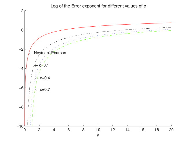
Figure 2: Computation of the logarithm of the error exponent ${\mathcal{E}}$ associated to the test $T_{N}$ for different values of $c$ (with ${\mathcal{E}}_{\rho}$ defined for $\rho\geq\sqrt{c}$ and ${\mathcal{E}}_{\rho}\,|_{\rho=\sqrt{c}}=0$), and comparison with the optimal result (Neyman-Pearson) obtained in the case where all the parameters are perfectly known.

In Figure 3, we compare the Error Exponent curves of both tests $T_{N}$ and $U_{N}$. The analytic expressions provided in 2 and 3 for the Error Exponent curves have been used to plot the curves. The asymptotic comparison clearly underlines the gain of using test $T_{N}$.

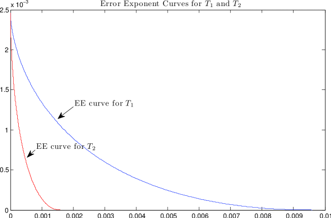
Figure 3: Error Exponent curves associated to the tests $T_{N}$ ($T_{1}$) and $U_{N}$ ($T_{2}$) in the case where $c=\frac{1}{5}$ and $\rho=10\,dB$. Each point of the curve corresponds to a given error exponent under $H_{0}$ ($X$ axis) and its counterpart error exponent under $H_{1}$ ($Y$ axis) as described in Theorem 2-(2) for $T_{N}$ and Theorem 3-(2) for $U_{N}$.

Finally, we compare in Figure 4 the powers (computed by Monte-Carlo methods) of tests $T_{N}$ and $U_{N}$ for finite values of $N$ and $K$. We consider the case where $K=10$, $N=50$ and $\rho=1$ and plot the probability of error under $H_{0}$ versus the power of the test, that is $\alpha$ versus $\mathbb{P}_{1}(T_{N}\geq\gamma_{N})$ (resp. $\mathbb{P}_{1}(U_{N}\geq\gamma_{N})$) where $\gamma_{N}$ is fixed by the following condition:

$$\mathbb{P}_{0}(T_{N}\geq\gamma_{N})=\alpha\quad(\textrm{resp.}\ \mathbb{P}_{0}(U_{N}\geq\gamma_{N})=\alpha)\ .$$

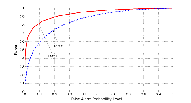
Figure 4: Simulated ROC curves for $T_{N}$ (test 1) and $U_{N}$ (test 2) in the case where $K=10$, $N=50$ and $\rho=10\,dB$.

VIII Conclusion

In this contribution, we have analyzed in detail the GLRT in the case where the noise variance and the channel are unknown. Unlike similar contributions, we have focused our efforts on the analysis of the error exponent by means of large random matrix theory and large deviation techniques. Closed-form expressions were obtained and enabled us to establish that the GLRT asymptotically outperforms the test based on the condition number, a fact that is supported by finite-dimension simulations. We also believe that the large deviations techniques introduced here will be of interest for the engineering community, beyond the problem addressed in this paper.

Acknowlegment

We thank Olivier Cappé for many fruitful discussions related to the GLRT.

Appendix A Proof of Lemma 1: Large deviations for $T_{N}$

The large deviations of the largest eigenvalue of large random matrices have already been investigated in various contexts, Gaussian Orthogonal Ensemble [49] and deformed Gaussian ensembles [21]. As mentionned in [21, Remark 1.2], the proofs of the latter can be extended to complex Wishart matrix models, that is random matrices $\bf{\hat{R}}$ under $H_{0}$ or $H_{1}$.

In both cases, the large deviations of $\lambda_{1}$ rely on a close study of the density of the eigenvalues, either given by (12) (under $H_{0}$) or by (19) for the spiked model (under $H_{1}$). The study of the spiked model, as it involves the study of the asymptotics of the spherical integral (see Lemma 3 below), is more difficult. We therefore focus on the proof of the LDP under $H_{1}$ (Lemma 1-(2)) and omit the proof of Lemma 1-(1). Once Lemma 1-(2) is proved, proving Lemma 1-(1) is a matter of bookkeeping, with the spherical integral removed at each step.

Recall that $\lambda_{1}\geq\cdots\geq\lambda_{K}$ are the ordered eigenvalues of $\hat{\bf R}$ and that $T_{N}$ is the statistics defined in (6).

In the sequel, we shall prove the upper bound of the LDP in Lemma 1-(2) (which gives also the upper bound in Lemma 1-(3)). The proof of the lower bound in Lemma 1-(3) requires more precise arguments than the lower bound of the LDP. One has indeed to study what happens at the vicinity of $\lambda^{+},$ which is a point of discontinuity of the rate function $I_{\rho}^{+}.$ Thus, we skip the proof of the lower bound of the LDP in Lemma 1-(2) to avoid repetition. Note that the proof of Lemma 1-(4) is a mere consequence of the fact that $T_{N}$ converges a.s. to $\lambda^{+}$ if $\rho\leq\sqrt{c},$ thus $\mathbb{P}_{1}(T_{N}<x_{N})$ converges to 1 whenever $x_{N}$ converges to $x>\lambda^{+}.$

For sake of simplicity and with no loss of generality as the law of $T_{N}$ does not depend on $\sigma,$ we assume all along this appendix that $\sigma^{2}=1.$ We first recall important asymptotic results for spherical integrals.

A-A Useful facts about spherical integrals

Recall that the joint distributions of the ordered eigenvalues under hypothesis $H_{0}$ and $H_{1}$ are respectively given by (12) and (19). In the latter, the so-called spherical integral (20) is introduced. We recall here results from [21] related to the asymptotic behaviour of the spherical integral in the case where one diagonal matrix is of rank one and the other has the limiting distribution $\mathbb{P}_{\check{\mathrm{M}}\mathrm{P}}$. We first introduce the function defined for $x\geq\lambda^{+}$ by:

$$J_{\rho}(x)=\left\{\begin{array}[]{ll}\frac{\rho}{c}-\log\left(\frac{\rho}{c(1+\rho)}\right)-{\bf F}^{+}(\lambda_{\mathrm{spk}}^{\infty}),&\textrm{ if }\rho\leq\sqrt{c}\textrm{ and }\lambda^{+}\leq x\leq\lambda_{\mathrm{spk}}^{\infty},\\ \frac{\rho x}{c(1+\rho)}-1-\log\left(\frac{\rho}{c(1+\rho)}\right)-{\bf F}^{+}(x),&\textrm{ otherwise.}\end{array}\right.$$ (60)

Consider a $K$-tuple $(x_{1},\cdots,x_{K})$ and denote by $\hat{\pi}_{K,{\bf x}}=\frac{1}{K-1}\sum_{i=2}^{N}\delta_{x_{2}}$ the empirical distribution associated to $(x_{2},\cdots,x_{K})$; let $d$ be a metric compatible with the topology of weak convergence of measures (for example the Dudley distance - see for instance [50]). A strong version of the convergence of the spherical integral in the exponential scale with speed $N$, established in [21] can be summarized in the following Lemma:

Lemma 3.

Assume that $N,K\to\infty$ and $\frac{K}{N}\to c\in(0,1)$ and let Assumption 1 hold true. Let $x_{1}\geq x_{2}\geq\cdots\geq x_{K}\geq 0$ and $\delta>0$. If, for $N$ large enough, $|x_{1}-x|\leq\delta$ and $d(\hat{\pi}_{K,\bf x},\mathbb{P}_{\check{\mathrm{M}}\mathrm{P}})\leq N^{-1/4}$ then:

$$\left|\frac{1}{N}\log I_{K}\left(\frac{N}{K}{\bf B}_{K},{\bf X}_{K}\right)-cJ_{\rho}(x)\right|\leq\delta,$$

where $J_{\rho}$ is given by (60), ${\bf B}_{K}={\rm diag}\left(\frac{\rho_{K}}{1+\rho_{K}},0,\ldots,0\right)$ and ${\bf X}_{K}=\mathrm{diag}(x_{1},\cdots,x_{K})$.

Recall that the spherical integral $I_{K}$, defined in (20), appears in the joint density (19) of the eigenvalues under $H_{1}$. Lemma 3 provides a simple asymptotic equivalent $cJ_{\rho}(x)$ of the normalized integral $N^{-1}\log I_{K}$. Roughly speaking, this will enable us to replace $I_{K}$ by the quantity $e^{-N\times cJ_{\rho}(x)}$ when establishing the large deviations of $\lambda_{1}$, which rely on a careful study of density (19).

A-B Proof of Lemma 1-(2)

In order to establish the LDP under hypothesis $H_{1}$ and condition $\rho>\sqrt{c}$, (that is the bounds (39) and (40)), we first notice that intervals $(x,x+\delta)$ for $x,\delta\in\mathbb{R}^{+}$ form a basis of the topology of $\mathbb{R}^{+}$. The LDP will be therefore a consequence of the following bounds:

• (Exponential tightness) there exists a function $f:\mathbb{R}^{+}\to\mathbb{R}^{+}$ going to infinity at infinity such that for all $N$,

  $$\mathbb{P}_{1}\left(\lambda_{1}\geq M\right)\ \leq\ e^{-Nf(M)}\ .$$ (61)

  Condition (61) is technical (see for instance [44, Lemma 1.2.18]): Instead of proving the large deviation upper bound for every closed set, the exponential tightness (61), if established, enables one to restrict to the compact sets.

• (Upper bound) For any $x$, for any $M$ such that $0<x<M,$

  $$\lim_{\delta\downarrow 0}\limsup_{N,K\to\infty}\frac{1}{N}\log\mathbb{P}_{1}\left(x\leq T_{N}\leq x+\delta,\,\lambda_{1}\leq M\right)\ \leq\ -I_{\rho}^{+}(x)\ ,$$ (62)

  Due to the exponential tightness, it is sufficient to establish the upper bound for compact sets. As each compact can be covered by a finite number of balls, it is therefore sufficient to establish upper estimate (62) in order to establish the LD upper bound.

• (Lower bound) For any $x$,

  $$\lim_{\delta\downarrow 0}\liminf_{N,K\to\infty}\frac{1}{N}\log\mathbb{P}_{1}\left(x\leq T_{N}\leq x+\delta\right)\ \geq\ -I_{\rho}^{+}(x)\ .$$ (63)

  The fact that (63) implies the LD lower bound (40) is standard in LD and can be found in [44, Chapter 1] for instance.

As the arguments are very similar to the ones developed in [21], we only prove in detail the upper bound (62). Proofs of (61) and (63) are left to the reader.

The idea is that the empirical measure $\hat{\pi}_{K,{\boldsymbol{\lambda}}}:=\frac{1}{K-1}\sum_{j=2}^{K}\delta_{\lambda_{j}}$ (of all but the largest eigenvalues) and the trace concentrate faster than the largest eigenvalue. In the exponential scale with speed $N$, $\hat{\pi}_{K,{\boldsymbol{\lambda}}}$ and the trace can be considered as equal to their limit, respectively $P_{\check{\mathrm{M}}{\mathrm{P}}}$ and 1. In particular, the deviations of $T_{N}$ arise from those of the largest eigenvalue and they both satisfy the same LDP with the same rate function $I_{\rho}^{+}$. We therefore isolate the terms depending on $\lambda_{1}$ and gather the others through their empirical measure $\hat{\pi}_{K,\boldsymbol{\lambda}}.$

Recall the notations introduced in (12) and (19) and let $x>\lambda^{+}$, $\delta>0$. Consider the following domain:

$${\mathcal{D}}=\left\{(x_{1},\cdots,x_{K})\in[0,M]^{K},\ \frac{Kx_{1}}{x_{1}+\cdots+x_{K}}\in(x,x+\delta)\right\}$$

For $N$ large enough:

$$\mathbb{P}_{1}(x\leq T_{N}\leq x+\delta,\,\,\lambda_{1}\leq M)=\int_{\mathcal{D}}dp_{K,N}^{1}(x_{1:K})$$

$$= \frac{1}{Z_{K,N}^{1}}\int_{\mathcal{D}}dx_{1}\,e^{-Nx_{1}}e^{(N-K)\log x_{1}}e^{2(K-1)\int\log(x_{1}-u)d\hat{\pi}_{K,{\bf x}}(u)}$$

$$\times I_{K}\left(\frac{N}{K}{\bf B}_{K},{\bf X}_{K}\right)\prod_{1<i<j}|x_{i}-x_{j}|^{2}e^{-N\sum_{j=2}^{K}x_{j}}\prod_{j=2}^{K}x_{j}^{N-K}d\,x_{2:K}\times{\boldsymbol{1}}_{(x_{1}\geq\dots\geq x_{K}\geq 0)}$$

$$= \frac{\left(1-\frac{1}{N}\right)^{(K-1)(N-1)}Z_{K-1,N-1}^{0}}{Z_{K,N}^{1}}\int_{\mathcal{D}}dx_{1}e^{-Nx_{1}}e^{(N-K)\log x_{1}}e^{2(K-1)\int\log(x_{1}-u)d\hat{\pi}_{K,{\bf y}}(u)}$$

$$\times I_{K}\left(\frac{N}{K}{\bf B}_{K},{\bf X}_{K}\right)dp_{K-1,N-1}^{0}(y_{2:K}),$$

where we performed the change of variables $y_{i}:=\frac{N}{N-1}x_{i}$ for $i=2:K$, and the related modifications $\hat{\pi}_{K,{\bf x}}\leftrightarrow\hat{\pi}_{K,{\bf y}}$ and ${\bf X}_{K}=\mathrm{diag}\left(x_{1},\frac{N-1}{N}y_{2},\cdots,\frac{N-1}{N}y_{2}\right)$. Note also that strictly speaking, the domain of integration ${\mathcal{D}}$ would express differently with the $y_{i}$’s and in particular, we should have changed constant $M$ which majorizes the $x_{i}$’s into a larger constant as the $y_{i}$’s can theoretically be slightly above $M$ - we keep the same notation for the sake of simplicity.

To proceed, one has to study the asymptotic behaviour of the normalizing constant:

$$\frac{\left(1-\frac{1}{N}\right)^{(K-1)(N-1)}Z_{K-1,N-1}^{0}}{Z_{K,N}^{1}}\ ,$$

which turns out to be difficult. Instead of establishing directly the bounds (61)-(63), we proceed as in [21] and establish similar bounds replacing the probability measures $\mathbb{P}_{1}$ by the measures $\mathbb{Q}_{1}$ defined as:

$$\mathbb{Q}_{1}:=\frac{Z_{K,N}^{1}}{Z_{K-1,N-1}^{0}\left(1-\frac{1}{N}\right)^{(K-1)(N-1)}}\mathbb{P}_{1}$$

and the rate function $I_{\rho}^{+}$ by the function $G_{\rho}$ defined by:

$$G_{\rho}(x)=\frac{x}{1+\rho}-(1-c)\log x-c{\bf F}^{+}(x)+c+c\log\left(\frac{\rho}{c(1+\rho)}\right)$$

for $x>\lambda^{+}$. Notice that these positive measures $\mathbb{Q}_{1}$ are not probability measures any more, and as a consequence, the function $G_{\rho}$ is not necessarily positive and its infimum might not be equal to zero, as it is the case for a rate function.

Writing the upper bound for $\mathbb{Q}_{1}$, we obtain:

$$\mathbb{Q}_{1}(x\leq T_{N}\leq x+\delta,\,\,\lambda_{1}\leq M)$$

$$\leq \int_{\mathcal{D}}dx_{1}e^{-N\Phi(x_{1},c_{N},\hat{\pi}_{K,{\bf y}})}I_{K}\left(\frac{N}{K}{\bf B}_{K},{\bf X}_{K}\right)dp_{K-1,N-1}^{0}(y_{2:K}),$$

where, for any compactly supported probability measure $\mu$ and any real number $y$ greater than the right edge of the support of $\mu,$

$$\Phi(y,c_{N},\mu)=-y+(1-c_{N})\log y+2c_{N}\int\log(y-\lambda)d\mu(\lambda).$$

Let us now localise the empirical measure $\hat{\pi}_{K,{\bf y}}$ around $\mathbb{P}_{\check{\mathrm{M}}\mathrm{P}}$ and the trace around 1. The continuity and convergence properties of the spherical integral recalled in Lemma 3 yield, for $K$ large enough:

$$\mathbb{Q}_{1}(x\leq T_{N}\leq x+\delta\ ,\ \lambda_{1}\leq M) \leq \int_{x}^{x+\delta}dx_{1}\int_{\mathcal{E}}e^{-N\Phi(x_{1},c_{N},\hat{\pi}_{K,{\bf y}})}e^{Nc(J_{\rho}(x_{1})+\delta)}dp_{K-1,N-1}^{0}(y_{2:K})$$ (64)

$$+4^{K}M^{N+K}e^{NM\frac{\rho_{K}}{1+\rho_{K}}}\int_{\mathcal{E}^{C}}dp_{K-1,N-1}^{0}(y_{2:K}),$$

with

$$\mathcal{E}:=\left\{(y_{2},\cdots,y_{K})\in[0,M]^{K-1},\ d(\hat{\pi}_{K,{\bf y}},\mathbb{P}_{\check{\mathrm{M}}\mathrm{P}})\leq\frac{1}{N^{1/4}}\quad\mathrm{and}\quad\frac{1}{K}\sum_{j=2}^{K}y_{j}\in\left[1-\delta^{2},1+\delta^{2}\right]\right\}.$$

The second term in (64) is easily obtained considering the fact that all the eigenvalues are less than $M$ so that for $1\leq j\leq K,$ $|x_{1}-x_{j}|\leq 2M,$ $x_{j}^{N-K}\leq M^{N-K}$ and $(UX_{K}U^{*})_{11}\leq M.$ Now, standard concentration results under $H_{0}$ yield that:

$$\limsup_{N,K\to\infty}\frac{1}{N}\log\mathbb{P}_{0}\left(\hat{\pi}_{K,{\bf\lambda}}\notin B(\mathbb{P}_{\check{\mathrm{M}}\mathrm{P}},N^{-1/4})\ \mathrm{or}\ \frac{1}{K}\sum_{j=2}^{K}\lambda_{j}\notin\left[1-\delta^{2},1+\delta^{2}\right]\right)=-\infty.$$

More precisely, one knows using [51] that the empirical measure $\frac{1}{K}\sum_{j=2}^{K}\lambda_{j}$ is close enough to its expectation and then using [52] one knows that the expectation is close enough to its limit $\mathbb{P}_{\check{\mathrm{M}}\mathrm{P}}.$ The arguments are detailed in the Wigner case in [21] and we do not give more details here.

As $c_{N}\to c$ for $N,K\to\infty$, $c\mapsto\Phi(y,c,\mu)$ is continuous and $\mu\mapsto\Phi(y,c,\mu)$ is lower semi-continuous, we obtain:

$$\limsup_{N,K\to\infty}\frac{1}{N}\log\mathbb{Q}_{1}(x\leq\lambda_{1}\leq x+\delta\ ,\ \lambda_{1}\leq M)\ \leq\ \sup_{u\in[x,x+\delta]}\left(\Phi(u,c,P_{\check{\mathrm{M}}{\mathrm{P}}})+cJ_{\rho}\left(u\right)\right)+2\delta.$$

By continuity in $u$ of the two involved functions, we finally get:

$$\lim_{\delta\downarrow 0}\limsup_{N,K\to\infty}\frac{1}{N}\log\mathbb{Q}_{1}(x\leq\lambda_{1}\leq x+\delta\ ,\ \lambda_{1}\leq M)\ \leq\ \Phi(x,c,\mathbb{P}_{\check{\mathrm{M}}\mathrm{P}})+cJ_{\rho}\left(x\right)=G_{\rho}(x)\ ,$$

and the counterpart of Eq. (62) is proved for $\mathbb{Q}_{1}$ and function $G_{\rho}$. The proof of the lower bound is quite similar and left to the reader. It remains now to recover (62). As $\mathbb{P}_{1}$ is a probability measure and the whole space $\mathbb{R}^{+}$ is both open and closed, an application of the upper and lower bounds for $\mathbb{Q}_{1}$ immediately yields:

$$\liminf_{N,K\to\infty}\frac{1}{N}\log\frac{Z_{K,N}^{1}}{Z_{K-1,N-1}^{0}\left(1-\frac{1}{N}\right)^{(K-1)(N-1)}}\mathbb{P}_{1}(T_{N}\in\mathbb{R}^{+})$$ (65)

$$= \limsup_{N,K\to\infty}\frac{1}{N}\log\frac{Z_{K,N}^{1}}{Z_{K-1,N-1}^{0}\left(1-\frac{1}{N}\right)^{(K-1)(N-1)}}\mathbb{P}_{1}(T_{N}\in\mathbb{R}^{+})$$

$$= \lim_{N,K\to\infty}\frac{1}{N}\log\frac{Z_{K,N}^{1}}{Z_{K-1,N-1}^{0}\left(1-\frac{1}{N}\right)^{(K-1)(N-1)}}$$

$$= -\inf_{\mathbb{R}^{+}}G_{\rho}\ .$$

This implies that the LDP holds for $\mathbb{P}_{1}$ with rate function $G_{\rho}-\inf_{\mathbb{R}^{+}}G_{\rho}$.

It remains to check that $I_{\rho}^{+}=G_{\rho}-\inf_{\mathbb{R}^{+}}G_{\rho}$, which easily follows from the fact to be proved that:

$$\inf_{x\in[\lambda^{+},\infty)}G_{\rho}(x)=G_{\rho}(\lambda_{\mathrm{spk}}^{\infty})\ .$$ (66)

We therefore study the variations of $G_{\rho}$ over $[\lambda^{+},\infty)$. Note that $({\bf F}^{+})^{\prime}=-{\bf f}$, and thus that $G_{\rho}^{\prime}(x)=(1+\rho)^{-1}-(1-c)x^{-1}+c{\bf f}(x)$. Function ${\bf f}$ being a Stieltjes transform is increasing for $x>\lambda^{+}$, and so is $G_{\rho}^{\prime}$, whose limit at infinity is $(1+\rho)^{-1}$. Straightforward but involved computations using the explicit representation (69) for ${\bf f}$ yield that $G^{\prime}_{\rho}(\lambda_{\mathrm{spk}}^{\infty})=0$. Therefore, $G_{\rho}$ is decreasing on $[\lambda^{+},\lambda_{\mathrm{spk}}^{\infty}]$ and increasing on $[\lambda_{\mathrm{spk}}^{\infty},\infty)$, and (66) is proved.

This concludes the proof of the upper bound in Lemma 1-(2). The proof of Lemma 1-(1) is very similar and left to the reader.

A-C Proof of Lemma 1-(3)

The proof of this point requires an extra argument as we study the large deviations of $T_{N}$ near the point $(1+\sqrt{c})^{2}$ where the rate function is not continuous. In particular, the limit (55) does not follow from the LDP already established. As we shall see when considering $\mathbb{P}_{1}\left(T_{N}<(1+\sqrt{c_{N}})^{2}+\eta_{N}N^{-2/3}\right)$, the fact that the scale $(N^{-2/3})$ is the same as the one of the fluctuations of the largest eigenvalue of the complex Wishart model is crucial.

We detail the proof in the case when $\rho>\sqrt{c}$ and, as above, consider the positive measures $\mathbb{Q}_{1}$. We need to prove that:

$$\liminf_{N,K\rightarrow\infty}\frac{1}{N}\log\mathbb{Q}_{1}\left(T_{N}<(1+\sqrt{c_{N}})^{2}+\frac{\eta}{N^{2/3}}\right)\geq-G_{\rho}(\lambda^{+}),\quad\eta\in\mathbb{R},$$ (67)

the other bound being a direct consequence of the LDP. As previously, we will carefully localize the various quantities of interest. Denote by $g_{N}(\eta)=(1+\sqrt{c_{N}})^{2}+\eta N^{-2/3}$ for $\eta\in\mathbb{R}$ and by $h_{N}(r)=1-rN^{-2/3}$ for $r>0$. Notice also that $\lambda_{1}\leq g_{N}(\eta)h_{N}(r)$ together with $\frac{1}{K-1}\sum_{j=2}^{K}\lambda_{j}>h_{N}(r)$ imply that $T_{N}<g_{N}(\eta)$. We shall also consider the further constraints:

$$g_{N}(\eta-1)h_{N}(r)\leq\lambda_{1}\quad\textrm{and}\quad\lambda_{2}<g_{N}(\eta-2)h_{N}(r)$$

which enable us to properly separate $\lambda_{1}$ from the support of $\hat{\pi}_{K,\boldsymbol{\lambda}}$. Now, with the localisation indicated above, we have for $N$ large enough,

$$\mathbb{Q}_{1}\left(T_{N}<g_{N}(\eta)\right)\ \geq\ \mathbb{Q}_{1}\bigg{(}g_{N}(\eta-1)h_{N}(r)\leq\lambda_{1}\leq g_{N}(\eta)h_{N}(r),\\ \frac{1}{K-1}\sum_{j=2}^{K}\lambda_{j}>h_{N}(r),\ \lambda_{2}<g_{N}(\eta-2)h_{N}(r),\ \hat{\pi}_{K,\boldsymbol{\lambda}}\in B(\mathbb{P}_{\check{\mathrm{M}}\mathrm{P}},N^{-1/4})\bigg{)}.$$

As previously, we consider the variables $y_{j}=\frac{N}{N-1}x_{j}$ for $2\leq j\leq K$ and obtain, with the help of Lemma 3:

$$\mathbb{Q}_{1}\left(T_{N}<g_{N}(\eta)\right)\geq\int_{g_{N}(\eta-1)h_{N}(r)}^{g_{N}(\eta)h_{N}(r)}dx_{1}\int_{\mathcal{F}}e^{-N\Phi(x_{1},c_{N},\hat{\pi}_{K,\bf y})}e^{Nc(J_{\rho}(x_{1})-\delta)}dp_{K-1,N-1}^{0}(y_{2:K})$$

with

$$\mathcal{F}:=\left\{(y_{2},\cdots,y_{K})\in\left[0,\frac{N\,g_{N}(\eta-2)\,h_{N}(r)}{N-1}\right]^{K-1},\right.\\ \left.\frac{1}{K-1}\sum_{j=2}^{K}y_{j}>\frac{N}{N-1}h_{N}(r),\hat{\pi}_{K,\bf y}\in B(\mathbb{P}_{\check{\mathrm{M}}\mathrm{P}},N^{-1/4})\right\}.$$

Therefore:

$$\mathbb{Q}_{1}\left(T_{N}<g_{N}(\eta)\right)\ \geq\ h_{N}(r)\ (g_{N}(\eta)-g_{N}(\eta-1))\ e^{N(G_{\rho}(\lambda^{+})-2\delta)}\mathbb{P}_{0}\left((\lambda_{2},\cdots,\lambda_{K})\in\mathcal{F}\right)$$

(recall that $G_{\rho}(x)=\Phi(x,c,\mathbb{P}_{\check{\mathrm{M}}\mathrm{P}})+cJ_{\rho}\left(x\right)$). Now, as $h_{N}(r)\ (g_{N}(\eta)-g_{N}(\eta-1))=(1-rN^{-2/3})N^{-2/3}$, its contribution vanishes at the LD scale:

$$\lim_{N\rightarrow\infty}\frac{1}{N}\log\left(h_{N}(r)\ (g_{N}(\eta)-g_{N}(\eta-1))\right)=0\ .$$

It remains to check that $\mathbb{P}_{0}\left((\lambda_{2},\cdots,\lambda_{K})\in\mathcal{F}\right)$ is bounded below uniformly in $N$. This will yield the convergence of $\frac{1}{N}\log\mathbb{P}_{0}\left((\lambda_{2},\cdots,\lambda_{K})\in\mathcal{F}\right)$ towards zero, hence (67). Consider:

$$\mathbb{P}_{0}\left((\lambda_{2},\cdots,\lambda_{K})\in\mathcal{F}^{c}\right)\leq\mathbb{P}_{0}\left(\hat{\pi}_{K,{\boldsymbol{\lambda}}}\notin B(\mathbb{P}_{\check{\mathrm{M}}\mathrm{P}},N^{-1/4})\right)\\ +\mathbb{P}_{0}\left(\frac{1}{K-1}\sum_{j=2}^{K}\lambda_{j}<\frac{N}{N-1}h_{N}(r)\right)+\mathbb{P}_{0}\left(\lambda_{2}>\frac{N}{N-1}g_{N}(\eta-2)h_{N}(r)\right)\ .$$

We have already used the fact that the first term goes to zero when $N$ grows to infinity. Recall that the fluctuations of $\frac{1}{K-1}\sum_{j=2}^{K}\lambda_{j}$ are of order $\frac{1}{N}$, therefore the second term also goes to zero as we consider deviations of order $N^{-2/3}$. Now, $N^{2/3}(\lambda_{2}-(1+\sqrt{c_{N}})^{2})$ converges in distribution to the Tracy-Widom law, therefore the last term converges to $F_{\rm TW}\left(\eta-2+r(1+\sqrt{c})^{2}\right)<1.$ This concludes the proof.

Appendix B Sketch of proof for Lemma 2: Large deviations for $U_{N}$

As stated in Remark 10, we shall first study the LDP for the joint quantity $(\lambda_{1},\lambda_{K})$. The purpose here is to outline the following convergence:

$$\frac{1}{N}\log\mathbb{P}\left(\lambda_{1}\in A,\lambda_{K}\in B\right)\xrightarrow[N,K\to\infty]{}-\inf_{x\in A}I^{+}_{\rho}(x)-\inf_{y\in B}I^{-}(x)\ ,$$

which is an illustrative way, although informal, to state the LDP for $(\lambda_{1},\lambda_{K})$ (see (41)).

Consider the quantity $\mathbb{P}\left(\lambda_{1}\in(\alpha_{1},\beta_{1}),\lambda_{K}\in(\alpha_{K},\beta_{K})\right)$. As we are interested in the deviations of $\lambda_{1}$ and $\lambda_{K}$, the interesting scenario is $\lambda^{+}\notin(\alpha_{1},\beta_{1})$ and $\lambda^{-}\notin(\alpha_{K},\beta_{K})$ (recall that $\lambda^{\pm}$ are the edgepoints of the support of Mar$\check{\textrm{c}}$enko-Pastur distribution). More precisely, the interesting case is when the deviations of the extreme eigenvalue occur outside of the bulk: $\alpha_{1}>\lambda^{+}$ and $\beta_{K}<\lambda^{-}$; such deviations happen at the rate $e^{-N\times const.}$. The case where the deviations would occur within the bulk is unlikely to happen because it would enforce the whole eigenvalues to deviate from the limiting support of Mar$\check{\textrm{c}}$enko-Pastur distribution, which happens at the rate $e^{-N^{2}\times const.}$. Denote by $A=(\alpha_{1},\beta_{1})$ and $B=(\alpha_{K},\beta_{K})$.

$$\mathbb{P}\left(\lambda_{1}\in A,\lambda_{K}\in B\right)$$

$$= \frac{1}{Z_{K,N}^{1}}\int_{A\times\mathbb{R}^{(K-2)}\times B}1_{(\lambda_{1}\geq\cdots\geq\lambda_{K}\geq 0)}\prod_{1\leq i<j\leq K}(x_{i}-x_{j})^{2}$$

$$\qquad\qquad\qquad\times\prod_{j=1}^{K}x_{j}^{N-K}e^{-Nx_{j}}I_{K}\left(\frac{N}{K}B_{K},X_{K}\right)d\,x_{1:K}$$

$$= \int_{A}d\,x_{1}\ e^{2\sum_{j=2}^{K-1}\log(x_{1}-x_{j})}e^{(N-K)\log x_{1}-Nx_{1}}I_{K}\left(\frac{N}{K}B_{K},X_{K}\right)$$

$$\quad\times\int_{B}d\,x_{K}\ e^{2\sum_{i=2}^{K-1}\log(x_{i}-x_{K})}e^{(N-K)\log x_{K}-Nx_{K}}e^{2\log(x_{1}-x_{K})}$$

$$\quad\quad\times\frac{Z_{K-2,N-2}^{0}}{Z_{K,N}^{1}}\int_{x_{1}\geq x_{2}\geq\cdots\geq x_{K}}\prod_{j=2}^{K-1}e^{-2x_{j}}\prod_{j=2}^{K-1}\frac{x_{j}^{N-K}e^{-(N-2)x_{j}}}{Z_{K-2,N-2}^{0}}\prod_{2\leq i<j\leq K-1}(x_{i}-x_{j})^{2}d\,x_{2:K-1}$$

We shall now perform the following approximations:

$$\sum_{j=2}^{K-1}\log(x_{1}-x_{j}) \approx (K-2)\int\log(x_{1}-x)\mathbb{P}_{\check{\mathrm{M}}\mathrm{P}}(\,dx)\ =(K-2){\bf F}^{+}(x_{1})\ ,$$

$$\sum_{j=2}^{K-1}\log(x_{j}-x_{K}) \approx (K-2)\int\log(x-x_{K})\mathbb{P}_{\check{\mathrm{M}}\mathrm{P}}(\,dx)\ =(K-2){\bf F}^{-}(x_{K})\ ,$$

$$\sum_{j=2}^{K-1}x_{j} \approx (K-2)\int x\mathbb{P}_{\check{\mathrm{M}}\mathrm{P}}(\,dx)\ =(K-2)\ ,$$

$$I_{K}\left(\frac{N}{K}B_{K},X_{K}\right) \approx e^{NcJ_{\rho}(x_{1})}\ .$$

The three first approximations follow from the fact that $\frac{1}{K-2}\sum_{2}^{K-1}\delta_{x_{i}}\approx\mathbb{P}_{\check{\mathrm{M}}\mathrm{P}}$, the last one from Lemma 3. Plugging these approximations into the expression of $\mathbb{P}\left(\lambda_{1}\in A,\lambda_{K}\in B\right)$ yields:

$$\mathbb{P}\left(\lambda_{1}\in A,\lambda_{K}\in B\right)$$

$$\approx \int_{A}d\,x_{1}\ e^{2(K-2){\bf F}^{+}(x_{1})}e^{(N-K)\log x_{1}-Nx_{1}}e^{NcJ_{\rho}(x_{1})}$$

$$\quad\times\int_{B}d\,x_{K}\ e^{2(K-2){\bf F}^{-}(x_{K})}e^{(N-K)\log x_{K}-Nx_{K}}e^{2\log(x_{1}-x_{K})}$$

$$\quad\quad\times\frac{Z_{K-2,N-2}^{0}}{Z_{K,N}^{1}}e^{-2(K-2)}\int_{x_{1}\geq x_{2}\geq\cdots\geq x_{K}}\prod_{j=2}^{K-1}\frac{x_{j}^{N-K}e^{-(N-2)x_{j}}}{Z_{K-2,N-2}^{0}}\prod_{2\leq i<j\leq K-1}(x_{i}-x_{j})^{2}d\,x_{2:K-1}\ .$$

As $x_{1}\geq\alpha_{1}\geq\lambda^{+}$ and $x_{K}\leq\beta_{K}\leq\lambda^{-}$, the last integral goes to one as $K,N\to\infty$ and:

$$\mathbb{P}\left(\lambda_{1}\in A,\lambda_{K}\in B\right)$$

$$\approx \int_{A}d\,x_{1}\ e^{-N\left(\frac{2(K-2)}{N}{\bf F}^{+}(x_{1})-\left(1-\frac{K}{N}\right)\log x_{1}+x_{1}-cJ_{\rho}(x_{1})\right)}$$

$$\times\int_{B}d\,x_{K}\ e^{-N\left(\frac{2(K-2)}{N}{\bf F}^{-}(x_{K})-\left(1-\frac{K}{N}\right)\log x_{K}+x_{K}+\frac{2\log(x_{1}-x_{K})}{N}\right)}$$

$$\quad\times\frac{Z_{K-2,N-2}^{0}}{Z_{K,N}^{1}}e^{-2(K-2)}\ .$$

Recall that we are interested in the limit $N^{-1}\log\mathbb{P}\left(\lambda_{1}\in A,\lambda_{K}\in B\right)$. The last term will account for a constant $\Upsilon$ (see for instance (65)):

$$\frac{1}{n}\log\left(\frac{Z_{K-2,N-2}^{0}}{Z_{K,N}^{1}}e^{-2(K-2)}\right)\quad\xrightarrow[N,K\to\infty]{}\quad\Upsilon\ .$$

The term $\frac{2\log(x_{1}-x_{K})}{N}$ within the exponential in the integral accounts for the interraction between $\lambda_{1}$ and $\lambda_{K}$ and its contribution vanishes at the desired rate. In order to evaluate the two remaining integrals, one has to rely on Laplace’s method (see for instance [53]) to express the leading term of the integrals (replacing $KN^{-1}$ by $c$ below):

$$\int_{A}d\,x_{1}\ e^{-N\left(2c{\bf F}^{+}(x_{1})-\left(1-c\right)\log x_{1}+x_{1}-cJ_{\rho}(x_{1})\right)} \approx e^{-N\inf_{x\in A}\left(2c{\bf F}^{+}(x)-\left(1-c\right)\log x+x-cJ_{\rho}(x)\right)}\ ,$$

$$\int_{B}d\,x_{K}\ e^{-N\left(2c{\bf F}^{-}(x_{K})-\left(1-c\right)\log x_{K}+x_{K}-cJ_{\rho}(x_{K})\right)} \approx e^{-N\inf_{y\in B}\left(2c{\bf F}^{-}(y)-\left(1-c\right)\log y+y\right)}\ .$$

Finally, we get the desired limit:

$$\frac{1}{N}\log\mathbb{P}\left\{\lambda_{1}\in A,\lambda_{K}\in B\right\}\xrightarrow[N,K\to\infty]{}-\inf_{x\in A}\Phi^{+}(x)-\inf_{y\in B}\Phi^{-}(y)+\Upsilon\ ,$$

where

$$\Phi^{+}(x) = 2c{\bf F}^{+}(x)-\left(1-c\right)\log x+x-cJ_{\rho}(x)\ ,$$

$$\Phi^{-}(y) = 2c{\bf F}^{-}(y)-\left(1-c\right)\log y+y\ .$$

It remains to replace $J_{\rho}$ by its expression (60) and to spread the constant $\Upsilon$ over $\Phi^{+}$ and $\Phi^{-}$, which are not a priori rate functions (recall that a rate function is nonnegative). If $\lambda^{-}\in B$, then the event $\{\lambda_{K}\in B\}$ is “typical” and no deviation occurs, otherwise stated, the rate function $I^{-}$ should satisfy $I^{-}(\lambda^{-})=0$. Similarly, $I_{0}^{+}(\lambda^{+})=0$ under $H_{0}$ and $I_{\rho}^{+}(\lambda_{\mathrm{spk}}^{\infty})=0$ under $H_{1}$. Necessarily, $\Upsilon$ should write $\Upsilon=\Phi(\lambda^{-})+\Phi(\lambda^{+})$ under $H_{0}$ (resp. $\Upsilon=\Phi(\lambda^{-})+\Phi(\lambda_{\mathrm{spk}}^{\infty})$ under $H_{1}$) and the rate functions should be given by: $I^{-}=\Phi^{-}-\Phi(\lambda^{-})$, $I_{0}^{+}=\Phi^{+}-\Phi(\lambda^{+})$ under $H_{0}$ (resp. $I_{\rho}^{+}=\Phi^{+}-\Phi(\lambda_{\mathrm{spk}}^{\infty})$ under $H_{1}$), which are the desired results.

We have proved (informally) that the LDP holds true for $(\lambda_{1},\Lambda_{K})$ with rate function $I_{0/\rho}^{+}(x)+I^{-}(y)$. The contraction principle [44, Chap. 4] immediatly yields the LDP for the ratio $\frac{\lambda_{1}}{\lambda_{K}}$ with rate function:

$$\Gamma_{0/\rho}(t)=\inf_{(x,y),\frac{x}{y}=t}\{I^{+}_{0/\rho}(x)+I^{-}(y)\}\ ,$$ (68)

which is the desired result. We provide here intuitive arguments to understand this fact.

For this, interpret the value of the rate function $I_{\rho}^{+}(x)$ as the cost associated to a deviation of $\lambda_{1}$ (under $H_{1}$) around $x$: $\mathbb{P}\{\lambda_{1}\in(x,x+dx)\}\approx e^{-NI^{+}_{\rho}(x)}$. If a deviation occurs for the ratio $\frac{\lambda_{1}}{\lambda_{K}}$, say $\frac{\lambda_{1}}{\lambda_{K}}\in(t,t+dt)$ where $t>\frac{\lambda_{\mathrm{spk}}^{\infty}}{\lambda^{-}}$ (which is the typical behaviour of $U_{N}$ under $H_{1}$), then necessarily $\lambda_{1}$ must deviate around some value $ty$, so does $\lambda_{K}$ around some value $y$, so that the ratio is around $t$. In terms of rate functions, the cost of the joint deviation $(\lambda_{1}\approx ty,\lambda_{K}\approx y)$ is $I^{+}_{\rho}(ty)+I^{-}(y)$. The true cost associated to the deviation of the ratio will be the minimum cost among all these possible joint deviations of $\lambda_{1}$ and $\lambda_{K}$, hence the rate function (68).

Appendix C Closed-form expressions for functions $\mathbf{f}$, $\mathbf{F}^{+}$ and $\mathbf{F}^{-}$

Consider the Stieltjes transform $\mathbf{f}$ of Mar$\check{\textrm{c}}$enko-Pastur distribution:

$$\mathbf{f}(z)=\int\frac{\mathbb{P}_{\check{\mathrm{M}}\mathrm{P}}(d\lambda)}{\lambda-z}\ .$$

We gather without proofs a few facts related to $\mathbf{f}$, which are part of the folklore.

Lemma 4 (Representation of $\mathbf{f}$).

The following hold true:

1. Function ${\bf f}$ is analytic in $\mathbb{C}-[\lambda^{-},\lambda^{+}]$.

2. If $z\in\mathbb{C}-[\lambda^{-},\lambda^{+}]$ with $\Re(z)\geq\frac{\lambda^{+}+\lambda^{-}}{2}$, then

   $${\bf f}(z)=\frac{(1-z-c)+\sqrt{(1-z-c)^{2}-4cz}}{2cz}\ ,$$

   where $\sqrt{z}$ stands for the principal branch of the square-root.

3. If $z\in\mathbb{C}-[\lambda^{-},\lambda^{+}]$ with $\Re(z)<\frac{\lambda^{+}+\lambda^{-}}{2}$, then

   $${\bf f}(z)=\frac{(1-z-c)-\sqrt{(1-z-c)^{2}-4cz}}{2cz}\ ,$$

   where $-\sqrt{z}$ stands for the branch of the square-root whose image is $\{z\in\mathbb{C},\ \Re(z)\leq 0\}.$

4. As a consequence, the following hold true:

   $$\quad{\bf f}(x) = \frac{(1-x-c)+\sqrt{(1-x-c)^{2}-4cx}}{2cx}\quad\textrm{if}\quad x\geq\lambda^{+}\ ,$$ (69)

   $$\quad{\bf f}(x) = \frac{(1-x-c)-\sqrt{(1-x-c)^{2}-4cx}}{2cx}\quad\textrm{if}\quad 0\leq x\leq\lambda^{-}\ .$$ (70)

5. Consider the following function $\tilde{\mathbf{f}}(z)=c\mathbf{f}(z)-\frac{1-c}{z}$. Functions $\mathbf{f}$ and $\tilde{\mathbf{f}}$ satisfy the following system of equations:

   $$\left\{\begin{array}[]{lcl}\mathbf{f}(z)&=&-\frac{1}{z(1+\tilde{\mathbf{f}}(z))}\\ \tilde{\mathbf{f}}(z)&=&-\frac{1}{z(1+c\mathbf{f}(z))}\end{array}\right.\ ,$$ (71)

Recall the definition (33) and (53) of function $\mathbf{F}^{+}$ and $\mathbf{F}^{-}$. In the following lemma, we provide closed-form formulas of interest.

Lemma 5.

The following identities hold true:

1. Let $x\geq\lambda^{+},$ then

   $$\mathbf{F}^{+}(x)=\log(x)+\frac{1}{c}\log(1+c\mathbf{f}(x))+\log(1+\tilde{\mathbf{f}}(x))+x\mathbf{f}(x)\tilde{\mathbf{f}}(x)\ .$$

2. Let $0\leq x\leq\lambda^{-},$ then

   $$\mathbf{F}^{-}(x)=\log(x)+\frac{1}{c}\log(1+c\mathbf{f}(x))+\log(-(1+\tilde{\mathbf{f}}(x)))+x\mathbf{f}(x)\tilde{\mathbf{f}}(x)\ .$$

Proof.

Consider the case where $x\geq\lambda^{+}$. First write

$$\log(x-y)=\log(x)+\int_{x}^{\infty}\left(\frac{1}{u}+\frac{1}{y-u}\right)\,du\ .$$

Integrating with respect with $\mathbb{P}_{\check{\mathrm{M}}\mathrm{P}}$ and applying Funini’s theorem yields:

$$\int\log(x-y)\mathbb{P}_{\check{\mathrm{M}}\mathrm{P}}(\,dy)=\log(x)+\int_{x}^{\infty}\left(\frac{1}{u}+\mathbf{f}(u)\right)\,du$$

in the case where $x>\lambda^{+}$. Recall that $\mathbf{f}$ and $\tilde{\mathbf{f}}$ are holomorphic functions over $\mathbb{C}-(\{0\}\cup[\lambda^{-},\lambda^{+}])$ and satisfy system (71) (notice in particular that $1+c\mathbf{f}$ and $1+\tilde{\mathbf{f}}$ never vanish). Using the first equation of (71) implies that:

$$\int\log(x-y)\mathbb{P}_{\check{\mathrm{M}}\mathrm{P}}(\,dy)=\log(x)-\int_{x}^{\infty}\mathbf{f}(u)\tilde{\mathbf{f}}(u)\,du\ .$$ (72)

Consider $\Gamma(u,\mathbf{f},\tilde{\mathbf{f}})=\frac{1}{c}\log(1+c\mathbf{f})+\log(1+\tilde{\mathbf{f}})+u\mathbf{f}\tilde{\mathbf{f}}$. By a direct computation of the derivative, we get:

$$\frac{d}{du}\Gamma(u,\mathbf{f}(u),\tilde{\mathbf{f}}(u)) = \mathbf{f}^{\prime}\left(\frac{1}{1+c\mathbf{f}}+u\tilde{\mathbf{f}}\right)+\tilde{\mathbf{f}}^{\prime}\left(\frac{1}{1+\tilde{\mathbf{f}}}+u\mathbf{f}\right)+\mathbf{f}\tilde{\mathbf{f}}$$

$$= \mathbf{f}(u)\tilde{\mathbf{f}}(u)\ .$$

Hence

$$\int_{x}^{\infty}\mathbf{f}(u)\tilde{\mathbf{f}}(u)\,du = \left[\frac{1}{c}\log(1+c\mathbf{f})+\log(1+\tilde{\mathbf{f}})+u\mathbf{f}\tilde{\mathbf{f}}\right]_{x}^{\infty}$$

$$= -\left(\frac{1}{c}\log(1+c\mathbf{f}(x))+\log(1+\tilde{\mathbf{f}}(x))+x\mathbf{f}(x)\tilde{\mathbf{f}}(x)\right).$$

It remains to plug this identity into (72) to conclude. The representation of $\mathbf{F}^{-}$ can be established similarly.

∎

References

- [1] J. Mitola III and GQ Maguire Jr. Cognitive radio: making software radios more personal. IEEE Wireless Communications, 6:13–18, 1999.
- [2] S. Haykin. Cognitive radio: Brain-empowered wireless communications. IEEE Journal on Selected areas in Comm., 23, 2005.
- [3] M. Dohler, E. Lefranc, and A.H. Aghvami. Virtual antenna arrays for future wireless mobile communication systems. ICT, Beijing, China, 2002.
- [4] H. Urkowitz. Energy detection of unknown deterministic signals. Proc. of the IEEE, 55:523–531, 1967.
- [5] V. I. Kostylev. Energy detection of a signal with random amplitude. Proc IEEE Int. Conf. on Communications, New York City.
- [6] M. K. Simon, F. F. Digham, and M.-S. Alouini. On the energy detection of unknown signals over fading channels. ICC 2003 Conference Record, Anchorage, Alaska, 2003.
- [7] Z. Quan, S. Cui, A. H. Sayed, and H. V. Poor. Spatial-spectral joint detection for wideband spectrum sensing in cognitive radio networks. Proc. ICASSP, Las Vegas, 2008.
- [8] E.L. Lehman and J.P. Romano. Testing statistical hypotheses. Springer Texts in Statistics. Springer, 2006.
- [9] M. Wax and T. Kailath. Detection of signals by information theoretic criteria. IEEE Trans. on Signal, Speech, and Signal Processing, 33(2):387–392, April 1985.
- [10] P-J Chung, J. F. Böhme, C. F. Mecklenbräuker, and A. Hero. Detection of the number of signals using the benjamin-hochberg procedure. IEEE Trans. on Signal Processing, 55, 2007.
- [11] A. Taherpour, M. Nasiri-Kenari, and S. Gazor. Multiple antenna spectrum sensing in cognitive radios. IEEE Transactions on Wireless Communications, 9(2):814–823, 2010.
- [12] X. Mestre. Improved estimation of eigenvalues and eigenvectors of covariance matrices using their sample estimates. IEEE Trans on Inform. Theory, 54(11):5113–5129, Nov. 2008.
- [13] X. Mestre. On the asymptotic behavior of the sample estimates of eigenvalues and eigenvectors of covariance matrices. IEEE Trans. on Signal Processing, 56(11):5353–5368, Nov. 2008.
- [14] S. Kritchman and B. Nadler. Determining the number of components in a factor model from limited noisy data. Chemometrics and Intelligent Laboratory Systems, 2008, 1932, 94.
- [15] S. Kritchman and B. Nadler. Non-parametric detection of the number of signals: Hypothesis testing and random matrix theory. in press in IEEE Transactions Signal Processing, 2009.
- [16] J. Silverstein and P. Combettes. Signal detection via spectral theory of large dimensional random matrices. IEEE Transactions on Signal Processing, 40(8):2100–2105, 1992.
- [17] R. Couillet and M. Debbah. A Bayesian Framework for Collaborative Multi-Source Signal Detection. IEEE Transactions on Signal Processing (under review), 2010. arxiv:0811.0764.
- [18] N. Raj Rao, J. A. Mingo, R. Speicher, and A. Edelman. Statistical eigen-inference from large Wishart matrices. Ann. Statist., 36(6):2850–2885, 2008.
- [19] N. Raj Rao and J. Silverstein. Fundamental limit of sample generalized eigenvalue based detection of signals in noise using relatively few signal-bearing and noise-only samples. arXiv:0902.4250, 2009.
- [20] I. M. Johnstone. On the distribution of the largest eigenvalue in principal components analysis. Ann. Statist., 29(2):295–327, 2001.
- [21] M. Maida. Large deviations for the largest eigenvalue of rank one deformations of Gaussian ensembles. Electron. J. Probab., 12:1131–1150 (electronic), 2007.
- [22] Y. H. Zeng and Y. C. Liang. Eigenvalue based spectrum sensing algorithms for cognitive radio. to appear in IEEE Trans on Communications volume=arXiv:0804.2960v1.
- [23] L. S. Cardoso, M. Debbah, P. Bianchi, and J. Najim. Cooperative Spectrum Sensing Using Random Matrix Theory. Proceedings of ISPWC, 2008.
- [24] F. Penna, R. Garello, and M. A. Spirito. Cooperative Spectrum Sensing based on the Limiting Eigenvalue Ratio Distribution in Wishart Matrices. IEEE Communication Letters, submitted, 2009.
- [25] T. Abbas, N-K Masoumeh, and G. Saeed. Multiple antenna spectrum sensing in cognitive radios. submitted to IEEE Transactions on Wireless Communications, 2009.
- [26] T. W. Anderson. Asymptotic theory for principal component analysis. J. Math. Stat., 34:122–148, 1963.
- [27] A. W. van der Vaart. Asymptotic statistics, volume 3 of Cambridge Series in Statistical and Probabilistic Mathematics. Cambridge University Press, Cambridge, 1998.
- [28] M. L. Mehta. Random matrices, volume 142 of Pure and Applied Mathematics (Amsterdam). Elsevier/Academic Press, Amsterdam, third edition, 2004.
- [29] G. Anderson, A. Guionnet, and O. Zeitouni. An Introduction to Random Matrices. Cambridge Studies in Advanced Mathematics. Cambridge University Press, 2009.
- [30] R. J. Muirhead. Aspects of multivariate statistical theory. John Wiley & Sons Inc., New York, 1982. Wiley Series in Probability and Mathematical Statistics.
- [31] P. Koev. Random Matrix statistics toolbox. http://math.mit.edu/ plamen/software/rmsref.html.
- [32] P. Koev and A. Edelman. The efficient evaluation of the hypergeometric function of a matrix argument. Math. Comp., 75(254):833–846 (electronic), 2006.
- [33] J. Mitola. Cognitive Radio An Integrated Agent Architecture for Software Defined Radio. PhD thesis, Royal Institute of Technology (KTH), May 2000.
- [34] V. A. Marčenko and L. A. Pastur. Distribution of eigenvalues in certain sets of random matrices. Mat. Sb. (N.S.), 72 (114):507–536, 1967.
- [35] G. Ben Arous and A. Guionnet. Large deviations for Wigner’s law and Voiculescu’s non-commutative entropy. Probab. Theory Related Fields, 108(4):517–542, 1997.
- [36] B. Nadler. On the distribution of the ratio of the largest eigenvalue to the trace of a wishart matrix. submitted to the Annals of Statistics, 2010. available at http://www.wisdom.weizmann.ac.il/nadler/.
- [37] C. A. Tracy and H. Widom. Level-spacing distributions and the Airy kernel. Comm. Math. Phys., 159(1):151–174, 1994.
- [38] C. A. Tracy and H. Widom. On orthogonal and symplectic matrix ensembles. Comm. Math. Phys., 177(3):727–754, 1996.
- [39] A. Bejan. Largest eigenvalues and sample covariance matrices. tracy-widom and painleve ii: computational aspects and realization in s-plus with applications. http://www.vitrum.md/andrew/TWinSplus.pdf, 2005.
- [40] F. Bornemann. Asymptotic independence of the extreme eigenvalues of GUE. arXiv:0902.3870, 2009.
- [41] J. Baik and J. Silverstein. Eigenvalues of large sample covariance matrices of spiked population models. J. Multivariate Anal., 97(6):1382–1408, 2006.
- [42] A. W. Van der Vaart. Asymptotic Statistics, chapter 14. Cambridge Univ. Press., 1998.
- [43] P. J. Bickel and P. W. Millar. Uniform convergence of probability measures on classes of functions. Statist. Sinica, 2(1):1–15, 1992.
- [44] A. Dembo and O. Zeitouni. Large Deviations Techniques And Applications. Springer Verlag, New York, second edition, 1998.
- [45] Y. Q. Yin, Z. D. Bai, and P. R. Krishnaiah. On the limit of the largest eigenvalue of the large-dimensional sample covariance matrix. Probab. Theory Related Fields, 78(4):509–521, 1988.
- [46] Z. D. Bai and Y. Q. Yin. Limit of the smallest eigenvalue of a large-dimensional sample covariance matrix. Ann. Probab., 21(3):1275–1294, 1993.
- [47] P. Bianchi, M. Debbah, and J. Najim. Asymptotic independence in the spectrum of the gaussian unitary ensemble. arXiv:0811.0979.
- [48] P.-N. Chen. General Formulas For The Neyman-Pearson Type-II Error Exponent Subject To Fixed And Exponential Type-I Error Bounds. IEEE Transactions on Information Theory, 42(1):316–323, 1996.
- [49] G. Ben Arous, A. Dembo, and A. Guionnet. Aging of spherical spin glasses. Probab. Theory Related Fields, 120(1):1–67, 2001.
- [50] R. M. Dudley. Real analysis and probability, volume 74 of Cambridge Studies in Advanced Mathematics. Cambridge University Press, Cambridge, 2002. Revised reprint of the 1989 original.
- [51] A. Guionnet and O. Zeitouni. Concentration of the spectral measure for large matrices. Electron. Comm. Probab., 5:119–136 (electronic), 2000.
- [52] Z. D. Bai. Convergence rate of expected spectral distributions of large random matrices. II. Sample covariance matrices. Ann. Probab., 21(2):649–672, 1993.
- [53] J. Dieudonné. Infinitesimal calculus. Hermann, Paris, 1971. Translated from the French.