Revisit of Tension in Recent SNIa Datasets
Abstract
Although today there are many observational methods, Type Ia supernovae (SNIa) is still one of the most powerful tools to probe the mysterious dark energy (DE). The most recent SNIa datasets are the 307 SNIa “Union” dataset [37] and the 397 SNIa “Constitution” dataset [23]. In a recent work [87], Wei pointed out that both Union and Constitution datasets are in tension with the observations of cosmic microwave background (CMB) and baryon acoustic oscillation (BAO), and suggested that two truncated versions of Union and Constitution datasets, namely “UnionT” and “ConstitutionT”, should be used to constrain various DE models. But in [87], only the CDM model is used to select the outliers from the Union and the Constitution dataset. In principle, since different DE models may select different outliers, the truncation procedure should be performed for each different DE model. In the present work, by performing the truncation procedure of [87] for 10 different models, we demonstrate that the impact of different models is negligible, and the approach adopted in [87] is valid. Moreover, by using the 4 SNIa datasets mentioned above, as well as the observations of CMB and BAO, we perform best-fit analysis on the 10 models. It is found that: (1) For each DE model, the truncated SNIa datasets not only greatly reduce and , but also remove the tension between SNIa data and other cosmological observations. (2) The CMB data is very helpful to break the degeneracy among different parameters, and plays a very important role in distinguishing different DE models. (3) The current observational data are still too limited to distinguish all DE models.
pacs:
98.80.-k, 95.36.+xI Introduction
Observations of Type Ia supernovae (SNIa) [58, 55, 70, 34, 59], cosmic microwave background (CMB) [6, 65, 66, 50, 24, 35] and large scale structure (LSS) [67, 68, 69] all indicate the existence of dark energy (DE) driving the current accelerating expansion of the universe. The most obvious theoretical candidate of DE is the cosmological constant , but it is plagued with the fine-tuning problem and the coincidence problem [88, 89, 62, 10, 52, 49, 16]. There are also many dynamical DE models, such as quintessence [51, 57, 57, 101], phantom [9, 11], -essence [2, 15, 3], CPL [14, 42], tachyon [48, 5], hessence [80, 81], Chaplygin gas [33], generalized Chaplygin gas [7], holographic [38, 26, 27, 39, 40, 99], agegraphic [83, 84], holographic Ricci [20], Yang-Mills condensate [100, 92, 73, 74], etc. Although numerous theoretical models have been proposed in the past decade, the nature of DE still remains a mystery.
In recent years, the numerical study of DE, i.e. utilizing cosmological observations to constrain DE models, has become one of the most active fields in the modern cosmology [1, 76, 77, 79, 29, 30, 25, 94, 95, 12, 96, 97, 98, 71, 72, 43, 44, 82, 85, 86]. Although today there are many observational methods, SNIa is still one of the most powerful tools to probe the mysterious DE. In the past decade, many SNIa datasets, such as Gold04 [60], Gold06 [61], SNLS [4], ESSENCE [91], Davis [17], have been released, while the number and quality of SNIa have continually increased. The most recent SNIa datasets are “Union” [37] and “Constitution” [23], and they have been widely used in the literature [64, 41, 56, 28, 93, 13, 21, 22, 63, 45, 75]. However, these SNIa datasets are not always consistent with other types of cosmological observations, and are even in tension with other SNIa samples. For examples, in [31, 32, 46], the Gold04 dataset was shown to be inconsistent with the SNLS dataset: the SNLS dataset favors the CDM model, while the Gold04 dataset favors the dynamical DE model. In [47], by comparing the maximum likelihood fits of the CPL parameters (, ) given by different SNIa samples, Nesseris and Perivolaropoulos found that the Gold06 dataset is also in tension with the SNLS dataset. Moreover, they also investigated how to remove this tension. The method is simple. First, they fitted the CDM model to the whole 182 SNIa in the Gold06 dataset, and obtained the best-fit parameter value of CDM model (for SNIa data only). Then, they calculated the relative deviation to the best-fit CDM prediction, , for all the 182 data points. Here is the observational value of distance modulus, is the theoretical value of distance modulus given by the best-fit CDM model, and is the 1 error of distance modulus. By searching the SNIa samples satisfying , they isolated six SNIa that are mostly responsible for the tension. Further, by using the random truncation method, they demonstrated that these 6 SNIa are systematically different from the Gold06 dataset.
In a recent work, by comparing the maximum likelihood fits of the CPL parameters (, ), Wei [87] pointed out that both Union and Constitution dataset are also in tension with the observations of CMB and baryon acoustic oscillation (BAO). Moreover, he also investigated how to remove these tensions. By using the method of truncation of [47], Wei found out the main sources that are responsible for the tensions: for the Union set, there are 21 SNIa differing from the best-fit CDM prediction beyond (i.e. ); and for the Constitution set, there are 34 SNIa differing from the best-fit CDM prediction beyond . The specific limit of truncation (i.e. ) is chosen based on two considerations: first, the tension between SNIa samples and other observations can be completely removed; second, the number of usable SNIa can be preserved as much as possible (see [87] for details). By subtracting these outliers from the Union dataset and the Constitution dataset, respectively, two new SNIa datasets, “UnionT” and “ConstitutionT” (“T” stands for “truncated”), were obtained. Further, Wei argued that the UnionT and the ConstitutionT datasets are fully consistent with the other cosmological observations, and should be used to constrain various DE models. But in [87], only the CDM model is used to select the outliers from the Union and the Constitution dataset. Since different DE models may select different outliers, one may doubt whether the approach adopted in [87] is valid. In principle, the truncation procedure should be performed for each different DE model. Only if the impact of different models is negligible, one can conclude that the conclusion of Wei is correct. So in the present work, we shall consider 10 different models. The truncation procedure will be performed for all these 10 models, and the corresponding cosmological consequences will be explored.
This paper is organized as follows: In Section 2, we briefly describe 10 theoretical models considered in this work. In Section 3, we present the method of data analysis, as well as the SNIa datasets we used in this paper. By performing the truncation procedure of [87] for 10 different models, we demonstrate that the approach adopted in [87] is valid. In Section 4, we show the data fitting results of 10 models, and present the corresponding conclusions. Section 5 is a short summary. In this work, we assume today’s scale factor , so the redshift satisfies ; the subscript “0” always indicates the present value of the corresponding quantity, and the unit with is used.
II Models
For a spatially flat (the assumption of flatness is motivated by the inflation scenario) Friedmann-Robertson-Walker (FRW) universe with matter component and DE component , the Friedmann equation reads
| (1) |
where is the reduced Planck mass, and is the Hubble parameter. Using this formula, one can easily get
| (2) |
where is the Hubble constant, is the present fractional matter density, and key function is given by the specific DE model. Equivalently, we have
| (3) |
where is the fractional DE density. Clearly, different DE model will give different . In the following, we shall briefly describe the models considered in this work.
II.1 Single-parameter models
(1) The CDM model: The DE density is always a constant, i.e. the equation of state (EOS) , so
| (4) |
(2) The Dvali-Gabadadze-Porrati (DGP) model: For this modified gravity model, the form of is [18]
| (5) |
where is a constant, satisfies
| (6) |
(3) The agegraphic dark energy (ADE): The DE density is characterized by the conformal age of the universe [84],
| (7) |
where is a positive constant. The equation of motion for is given by [84]
| (8) |
As in [84], we choose the initial condition, , at , then Eq. (8) can be numerically solved. Substituting the results of Eq. (8) into Eq. (3), the key function can be obtained. Notice that once is given, can be naturally obtained by solving Eq. (8), so the ADE model is a single-parameter model.
II.2 Two-parameter models
(4) The XCDM model: DE has a constant EOS , then
| (9) |
(5) The Chaplygin gas (CG) model: The EOS of DE has the form [33]
| (10) |
where is a positive constant, and is the pressure of DE. From this assumption, one can get [33]
| (11) |
here is also a positive constant.
(6) The holographic dark energy (HDE) model: The DE density is characterized by the future event horizon of the universe [38],
| (12) |
where is a positive constant. The equation of motion for is given by [38]
| (13) |
Solving Eq. (13) numerically and substituting the corresponding results into Eq. (3), can be obtained.
II.3 Three-parameter models
(8) The linear parameterization (LP) model: The EOS of DE is parameterized as
| (16) |
where and are constants. Then
| (17) |
III Methodology
III.1 Data analysis
In this work we adopt statistics. For a physical quantity with experimentally measured value , standard deviation , and theoretically predicted value , the value is given by
| (22) |
The total is the sum of all s, i.e.
| (23) |
First, we consider the SNIa data that are given in terms of the distance modulus . The theoretical distance modulus is defined as
| (24) |
where with the Hubble constant in units of 100 km/s/Mpc, and in a flat universe the Hubble-free luminosity distance ( denotes the physical luminosity distance) is
| (25) |
where denotes the model parameters. The for the SNIa data is
| (26) |
where and are the observed value and the corresponding 1 error of distance modulus for each supernova, respectively. Parameter is a nuisance parameter but it is independent of the data and the dataset. Following [54], the minimization with respect to can be made trivially by expanding the of Eq. (26) with respect to as
| (27) |
where
| (28) |
| (29) |
| (30) |
Evidently, Eq. (26) has a minimum for at
| (31) |
Since , instead of minimizing we will minimize which is independent of the nuisance parameter .
Next, we consider constraints from the CMB and the LSS observations. For the CMB data, we use the CMB shift parameter , given by [8, 78]
| (32) |
where the redshift of recombination [36]. The measured value of has been updated to be from the WMAP7 observations [36]. For the LSS data, we use the BAO distance measurements obtained at and from the joint analysis of the 2dFGRS and SDSS data [53]. The BAO distance ratio was shown in [53] to be a relatively model independent quantity. Here is defined as
| (33) |
The total is given by
| (34) |
where is given by Eq. (31), and the latter two terms are defined as
| (35) |
and
| (36) |
The model parameters yielding a minimal is favored by the observations.
To compare different models, a statistical variable must be chosen. The is the simplest one, but it has difficulty to compare different models with different number of parameters. In this work, we will use as a model selection criterion, where is the degree of freedom defined as
| (37) |
here is the number of data, and is the number of free parameters. This model selection criterion has been widely used in the literature.
III.2 SNIa Datasets
Although today there are many observational methods, SNIa is still one of the most powerful tools to probe the mysterious DE. In the past decade, many SNIa datasets have been released, while the number and quality of SNIa have continually increased. In 2008, the Union dataset [37] was released. It includes the large samples of SNIa from the HST, SNLS and ESSENCE, and contains 307 samples: 250 high redshift SNIa () and 57 low redshift SNIa (). In 2009, the Constitution set [23] was released. It adds 90 low redshift samples. These two SNIa datasets have been widely used in the literature.
In a recent work [87], by comparing the maximum likelihood fits of the CPL parameters (, ), Wei pointed out that both Union and Constitution datasets are in tension not only with the observations of CMB and BAO, but also with the other SNIa datasets. Moreover, he also investigated how to remove these tensions. The method of Wei is as follows. First, he fitted the CDM model to all the data points in the specific SNIa dataset, and obtained the best-fit parameter value of CDM model (for SNIa data only). Then, he calculated the relative deviation to the best-fit CDM prediction, , for all the SNIa data points. By searching the SNIa samples satisfying , Wei get the main sources that are responsible for the tensions. For the Union set, there are 21 SNIa differing from the best-fit CDM prediction beyond , which is called “UnionOut” subset.
-
•
UnionOut subset (21 SNIa):
1992bs, 1995ac, 1999bm, 1997o, 2001hu, 1998ba, 04Pat, 05Red, 2002hr, 03D4au,
04D3cp, 03D1fc, 03D4dy, 03D1co, b010, d033, g050, g055, k430, m138, m226
For the Constitution set, There are 34 SNIa differing from the best-fit CDM prediction beyond , which is called “ConstitutionOut” subset.
-
•
ConstitutionOut subset (34 SNIa):
1992bs, 1992bp, 1995ac, 1999bm, 1996t, 1997o, 1995aq, 2001hu, 1998ba, 04Pat, 05Red,
2002hr, 03D4au, 04D3gt, 04D3cp, 03D4at, 03D1fc, 04D3co, 03D4dy, 04D3oe, 04D1ak,
03D1co, b010, d033, f076, g050, k430, m138, m226, sn01cp, sn02hd, sn03ic, sn07ca, sn07R
It should be mentioned that is chosen based on two considerations: first, the tension between SNIa samples and other observations can be completely removed; second, the number of usable SNIa can be preserved as much as possible. After taking into account these two factors, Wei found that is most appropriate for the truncation procedure. By subtracting these two subsets from the Union dataset and the Constitution dataset, respectively, two new SNIa samples, “UnionT” and “ConstitutionT”, were obtained. It is clear that UnionT has 286 SNIa samples, and ConstitutionT has 363 SNIa samples. Analyzing these two truncated datasets with CPL model, Wei [87] argued that they are fully consistent with the other cosmological observations.
But in [87], only the CDM model is used to select the outliers from the Union and the Constitution dataset. Since different DE models may select different outliers (i.e. different “UnionOut” and“ConstitutionOut” Samples), one may doubt whether the approach adopted in [87] is valid. In principle, the truncation procedure should be performed for each different DE model. Only if the impact of different models is negligible, one can conclude that the conclusion of Wei is correct. So in this work, we perform the truncation procedure for 10 different DE models. As in [87], we choose as the selection criterion. The results are shown in table 1 and table 2. From these two tables, it is seen that the difference among the outlier samples given by various models are very small, and the impact of different models is negligible. Therefore, the approach adopted in [87] is valid. Since the difference among the outlier samples given by various models are very small, for simplicity, in this work we just adopt the UnionT and the ConstitutionT SNIa samples given by [87]. To explore the corresponding cosmological consequences, in the following we shall study 10 models by using 4 SNIa datasets: Union, UnionT, Constitution and ConstitutionT.
| Model | Numbers of “UnionOut” samples for each model | Differences with the CDM UnionOut subset |
|---|---|---|
| CDM | None | |
| DGP | None | |
| ADE | None | |
| XCDM | +1999gd +f076 -05Red | |
| CG | +1999gd +f076 -05Red | |
| HDE | +1999gd +f076 -05Red | |
| RDE | +1999gd +f076 -05Red | |
| LP | +1999gd +f076 -1999bm -05Red -03D1co -k430 | |
| CPL | +1999gd +f076 -1999bm -05Red -03D1co | |
| GCG | +1999gd +f076 -05Red |
| Model | Numbers of “ConstitutionOut” samples for each model | Difference with the CDM ConstitutionOut subset |
|---|---|---|
| CDM | None | |
| DGP | None | |
| ADE | -sn07R | |
| XCDM | None | |
| CG | +1997aj -1992bp | |
| HDE | None | |
| RDE | None | |
| LP | +1997aj -1992bp -1999bm -03D4at | |
| CPL | +1997aj +sn02bf -1992bp -1999bm -sn07R | |
| GCG | +1997aj -1992bp |
IV Results and Conclusions
We will present the results of data fitting in this section. Using the Union, the UnionT, the Constitution and the ConstitutionT dataset, respectively, we list the and the for those 10 models, in table 3, table 4, table 5, and table 6. Here “SNIa” means only SNIa data is used in the analysis, “SNIa+BAO” means both SNIa data and BAO data are used, “SNIa+CMB” means both SNIa data and CMN data are used, and “SNIa+BAO+CMB” means all these three types of observational data are taken into account. The main conclusions are summarized as follows.
| Model | SNIa | SNIa+BAO | SNIa+CMB | SNIa+BAO+CMB |
|---|---|---|---|---|
| CDM | ||||
| DGP | ||||
| ADE | ||||
| XCDM | ||||
| CG | ||||
| HDE | ||||
| RDE | ||||
| LP | ||||
| CPL | ||||
| GCG |
| Model | SNIa | SNIa+BAO | SNIa+CMB | SNIa+BAO+CMB |
|---|---|---|---|---|
| CDM | ||||
| DGP | ||||
| ADE | ||||
| XCDM | ||||
| CG | ||||
| HDE | ||||
| RDE | ||||
| LP | ||||
| CPL | ||||
| GCG |
| Model | SNIa | SNIa+BAO | SNIa+CMB | SNIa+BAO+CMB |
|---|---|---|---|---|
| CDM | ||||
| DGP | ||||
| ADE | ||||
| XCDM | ||||
| CG | ||||
| HDE | ||||
| RDE | ||||
| LP | ||||
| CPL | ||||
| GCG |
| Model | SNIa | SNIa+BAO | SNIa+CMB | SNIa+BAO+CMB |
|---|---|---|---|---|
| CDM | ||||
| DGP | ||||
| ADE | ||||
| XCDM | ||||
| CG | ||||
| HDE | ||||
| RDE | ||||
| LP | ||||
| CPL | ||||
| GCG |
(1) For each DE model, the truncated SNIa datasets not only greatly reduce and , but also remove the tension between SNIa data and other cosmological observations.
Since it is too prolix to describe the results of all 10 models, in the following we will just discuss the HDE model as an example. From table 3 and table 4, we can see that the combined Union+BAO+CMB data gives a and a , while the combined UnionT+BAO+CMB data gives a and a . This means that by dropping the 21 outliers, The and the of the HDE model can reduce 106.867 and 0.299, respectively. From table 5 and table 6, similar results are obtained. The combined Constitution+BAO+CMB data gives a and a , while the combined ConstitutionT+BAO+CMB data gives a and a . This means that by dropping the 34 outliers, The and the of the HDE model can reduce 196.686 and 0.431, respectively. It should be pointed out that for all these 10 models, the UnionT and the ConstitutionT dataset can greatly reduce the corresponding and . Moreover, the decreasing margin of and for these 10 DE models are almost same.
To further verify this conclusion, we also adopt the method of random truncation used in [47, 87]. The method is very simple. First, we random select the outliers from the full Union dataset and the full Constitution dataset, respectively. Notice that the numbers of data points in these random “UnionOut” subsets are same as that in the original UnionOut samples, while the numbers of data points in these random “ConstitutionOut” subsets are same as that in the original ConstitutionOut samples. As in [47, 87], 500 random UnionOut subsets and 500 random ConstitutionOut subsets are selected. By subtracting these outliers from the Union dataset and the Constitution dataset, respectively, 500 random UnionT subsets and 500 random ConstitutionT subsets are obtained. Then, we perform best-fit analysis on the HDE model by using these random truncated SNIa subsets. Using the SNIa data only, we get the Mean of for 500 random UnionOut subsets and 500 random ConstitutionOut subsets, respectively. Notice that the full Union set gives a and the full Constitution set gives a , the differences between the of the full SNIa dataset and the Mean of of these random truncated SNIa subsets are also obtained. Next, we make a comparison for the original truncated SNIa subset and the random truncated SNIa subsets. The results are shown in table 7. It is found that the of the HDE model can reduce 5 by dropping 1 data point in the original truncated SNIa subset, but can only reduce 1 by dropping 1 data point in the random truncated SNIa subset. Therefore, the original UnionOut and ConstitutionOut subsets are systematically different from the full Union and Constitution datasets, and the original truncated supernova datasets provide a significantly better model fitting than the full SNIa datasets.
| The subset of outliers | or | |||
|---|---|---|---|---|
| The original UnionOut subset | 21 | |||
| 500 random UnionOut subsets | 21 (Mean) | (Mean) | (Mean) | (Mean) |
| The original ConstitutionOut subset | 34 | |||
| 500 random ConstitutionOut subsets | 34 (Mean) | (Mean) | (Mean) | (Mean) |
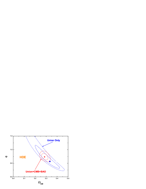
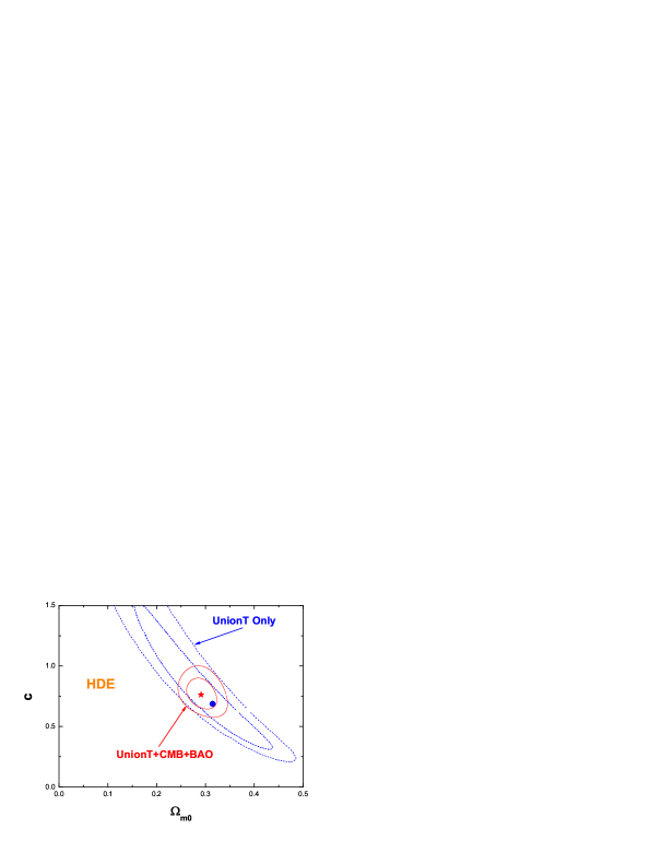
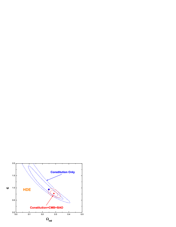
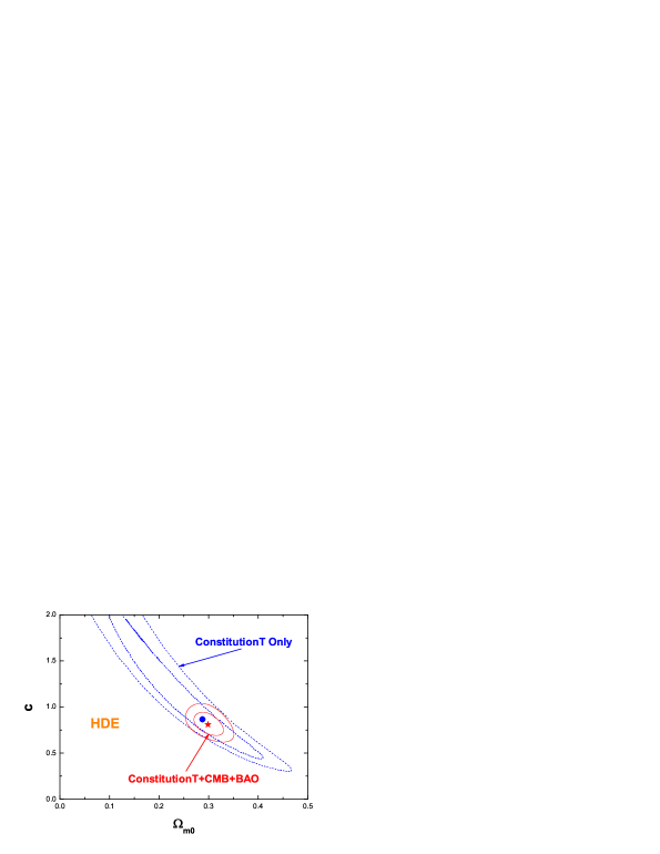
In [87], by performing the best-fit analysis on the CPL model, Wei argued that the UnionT and the ConstitutionT datasets are fully consistent with the other cosmological observations. To verify this conclusion, more theoretical models should be taken into account. Here we study the HDE model as an example. In Fig.1, we plot the and the confidence level (CL) contours for the HDE model, where the Union and the UnionT datasets are used, respectively. From this figure, we find that the best-fit point for the Union data is outside the confidence region given by the combined Union+BAO+CMB data, while the best-fit point for the UnionT data is inside the confidence region given by the combined UnionT+BAO+CMB data. This means that the UnionT dataset is very useful to remove the tension between SNIa data and other cosmological observations. In addition, we also use the Constitution and the ConstitutionT datasets to plot the CL contours for the HDE model in Fig.2. It is found that the best-fit point for the Constitution data is outside the confidence region given by the combined Constitution+BAO+CMB data, while the best-fit point for the ConstitutionT data is very close to the best-fit point for the combined ConstitutionT+BAO+CMB data. This means that the ConstitutionT dataset is also very helpful to remove the tension. Therefore, we conclude that the truncated SNIa datasets can remove the tension between SNIa data and other cosmological observations.
(2) The CMB data is very helpful to break the degeneracy among different parameters, and plays a very important role in distinguishing different DE models.
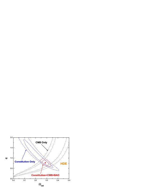
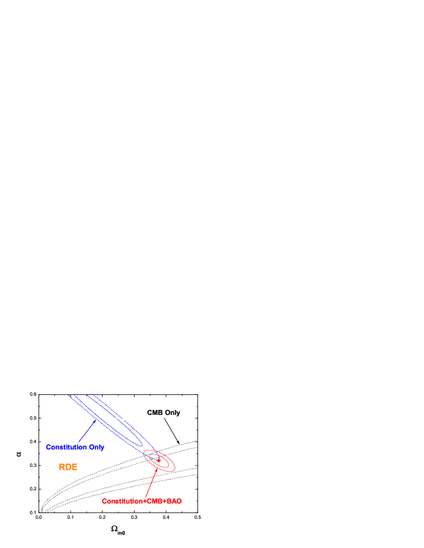
As an example, we will compare the HDE model with the RDE model. By using the Constitution SNIa data alone, the CMB data alone, and the combined Constitution+CMB+BAO data, respectively, we plot the and the CL contours for the HDE and the RDE model in Fig.3. From this figure, we find that the shapes of CL contours given by the CMB data alone are quite different from that given by the SNIa data alone, and the CMB data is very helpful to break the degeneracy among different parameters. As shown in the left panel, the CL contour of the HDE model given by the CMB data intersects to the CL contour of the HDE model given by the SNIa data; while in the right panel, the CL contour of the RDE model given by the CMB data does not intersect to the CL contour of the RDE model given by the SNIa data. This fact explains why the HDE model performs much better in fitting the combined Constitution+BAO+CMB data than the RDE model. Besides, we also check the effect of the BAO data, and find that the confidence region of the HDE model given by the BAO data alone can completely cover that given by the SNIa data. So the constraint given by the BAO data is quite weaker than that given by the SNIa and the BAO data. This conclusion can be further verified by using table 5. As seen in table 5, without adopting the CMB data, it is very difficult to distinguish the HDE Model from the RDE model. After adding the CMB data, it is seen that the of the HDE Model given by the SNIa+CMB data is 6.811 smaller than the of the RDE Model given by the SNIa+CMB data, while the of the HDE Model given by the combined SNIa+CMB+BAO data is 7.082 smaller than the of the RDE Model given by the combined SNIa+CMB+BAO data.
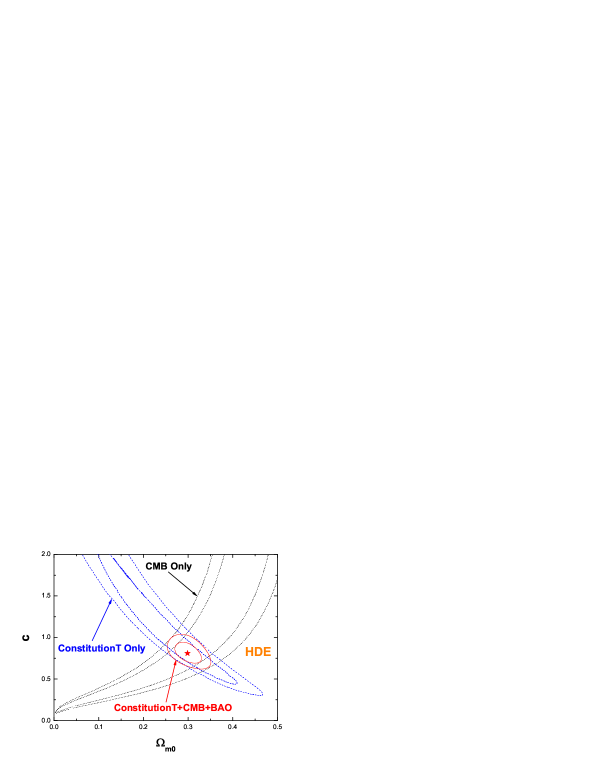
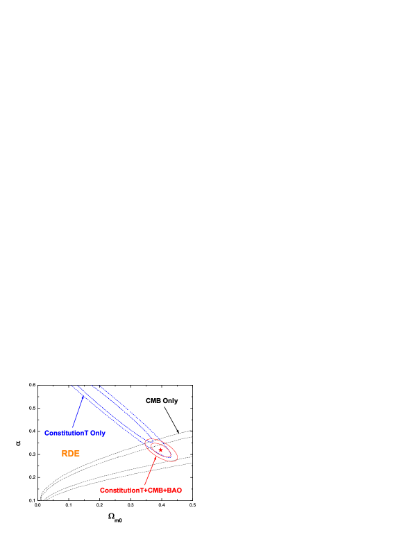
In addition, by using the ConstitutionT SNIa data alone, the CMB data alone, and the combined ConstitutionT+CMB+BAO data, respectively, we also plot the and the CL contours for the HDE and the RDE model in Fig.4. Again, we see that the CL contour of the HDE model given by the CMB data intersects to the CL contour of the HDE model given by the SNIa data, while the CL contour of the RDE model given by the CMB data does not intersect to the CL contour of the RDE model given by the SNIa data. This fact explains why the HDE model performs much better in fitting the combined ConstitutionT+BAO+CMB data than the RDE model. Therefore, the CMB data is very helpful to break the degeneracy among different parameters, and plays a very important role in distinguishing different DE models.
(3) The current observational data are still too limited to distinguish all DE models.
First, we discuss three kinds of two-parameter models: the XCDM model, the CG model, and the HDE model. As seen in table 5, the of these 3 models given by the combined Constitution+BAO+CMB data are 466.947, 466.891, and 467.384, respectively. That is to say, after taking into account the CMB data, the differences of the of these 3 models are still smaller than 1. Notice that this result also holds true in table 3, table 4, and table 6. Therefore, one cannot judge which DE model is better.
Then, we discuss three kinds of three-parameter models: the LP model, the CPL model, and the GCG model. As seen in table 5, the of these 3 models given by the combined Constitution+BAO+CMB data are 466.910, 466.902, 466.895, respectively, and the differences of the of these 3 models are even smaller than 0.1. Since this result also holds true in table 3, table 4, and table 6, it is also very difficult to distinguish these 3 models. Therefore, to distinguish DE models better, more high-quality observational data are needed.
V Summary
In this work, by performing the truncation procedure of [87] for 10 different models, we demonstrate that the approach adopted in [87] is valid. Moreover, by using the 4 SNIa datasets mentioned above, as well as the observations of CMB and BAO, we perform best-fit analysis on the 10 DE models. It is found that: (1) For each DE model, the truncated SNIa datasets not only greatly reduce and , but also remove the tension between SNIa data and other cosmological observations. (2) The CMB data is very helpful to break the degeneracy among different parameters, and plays a very important role in distinguishing different DE models. (3) The current observational data are still too limited to distinguish all DE models. These results provide a further support for Wei’s work, and indicate that the existence of biasing systematic errors in SNIa data should be taken into account seriously.
Acknowledgements
We are grateful to the reviewer for very useful and helpful suggestions. We also thank Qing-Guo Huang, Hao Wei and Xin Zhang, for helpful discussions. This work was supported by the NSFC grant No.10535060/A050207, a NSFC group grant No.10821504 and Ministry of Science and Technology 973 program under grant No.2007CB815401. Shuang Wang was also supported by a graduate fund of USTC.
References
- Albrecht et al. [2006] Albrecht, A. et al., 2006, arXiv:astro-ph/0609591
- Armendariz-Picon et al. [1999] Armendariz-Picon, C. et al., 1999, Phys. Lett. B 458, 209
- Armendariz-Picon et al. [2001] Armendariz-Picon, C. et al., 2001, Phys. Rev. D 63, 103510
- Astier et al. [2007] Astier, P. et al., 2007, Astron. Astrophys. 447, 31
- Bagla et al. [2003] Bagla, J.S. et al., 2003, Phys. Rev. D 67, 063504
- Bennet et al. [2003] Bennet, C.L. et al., 2003, ApJS. 148, 1
- Bento et al. [2002] Bento, M.C. et al., 2002, Phys. Rev. D 66, 043507
- Bond et al. [1997] Bond, J.R. et al., 1997, MNRAS. 291, L33
- Caldwell [2002] Caldwell, R.R., 2002, Phys. Lett. B 545, 23
- Carroll [2001] Carroll, S.M., 2001, Living Rev. Rel. 4, 1
- Carroll et al. [2003] Carroll, S.M. et al., 2003, Phys. Rev. D 68, 023509
- Chang et al. [2006] Chang, Z. et al., 2006, Phys. Lett. B 633, 14
- Chen et al. [2009] Chen, C.W. et al., 2009, Phys. Lett. B 682 267
- Chevallier and Polarski [2001] Chevallier, M. and Polarski, D., 2001, Int. J. Mod. Phys. D 10, 213
- Chiba et al. [2000] Chiba, T. et al., 2000, Phys. Rev. D 62, 023511
- Copeland et al. [2006] Copeland, E.J. et al., 2006, Int. J. Mod. Phys. D 15, 1753
- Davis et al. [2007] Davis, T. et al., 2007, ApJ. 666, 716
- Dvali et al. [2000] Dvali, G.R. et al., 2000, Phys. Lett. B 485, 208
- Eisenstein et al. [2005] Eisenstein, D.J. et al., 2005 ApJ. 633, 560
- Gao et al. [2009] Gao, C. et al., 2009, Phys. Rev. D 79, 043511
- [21] Gong, Y.G. and Li, T.J., 2010, Phys. Lett. B 683 241
- [22] Gong, Y.G. et al., 2010, JCAP 01 019
- Hicken et al. [2009] Hicken, M. et al., 2009, ApJ 700, 1097
- Hinshaw et al. [2007] Hinshaw, G. et al., 2007, ApJS 170, 263
- Huang and Gong [2004] Huang, Q.G. and Gong, Y.G., 2004 JCAP 0408, 006
- [26] Huang, Q.G. and Li, M., 2005, JCAP 0408, 013
- [27] Huang, Q.G. and Li, M., 2005, JCAP 0503, 001
- Huang et al. [2009] Huang, Q.G. et al., 2009, Phys. Rev. D 80 083515
- Huterer and Starkman [2003] Huterer, D. and Starkman, G., 2003 Phys. Rev. Lett. 90, 031301
- Huterer and Cooray [2005] Huterer, D. and Cooray, A., 2005, Phys. Rev. D 71, 023506
- Jassal et al. [2005] Jassal, H. et al., 2005, Phys. Rev. D 72,103503
- Jassal et al. [2006] Jassal, H. et al., 2006, arXiv:astro-ph/0601389, accepted for publication in MNRAS
- Kamenshchik et al. [2001] Kamenshchik, A.Y. et al., 2001, Phys. Lett. B 511 265
- Knop et al. [2003] Knop, R.A. et al., 2003, ApJ 598, 102
- Komatsu et al. [2009] Komatsu, E. et al., 2009, ApJS. 180, 3301
- Komatsu et al. [2010] Komatsu, E. et al., arXiv:1001.4538.
- Kowalski et al. [2008] Kowalski, M. et al., 2008 ApJ. 686, 749
- Li [2004] Li, M., 2004, Phys. Lett. B 603 1
- Li et al. [2008] Li, M. et al., 2008, JCAP 0805, 023
- [40] Li, M. et al., 2009, Commun. Theor. Phys. 51, 181
- [41] Li, M. et al., 2009, JCAP 0906, 036
- Linder [2003] Linder, E.V., 2003, Phys. Rev. Lett. 90, 091301
- [43] Ma, Y.Z. et al., 2009, Eur. Phys. J. C 60, 303
- [44] Ma, Y.Z. et al., 2009, arXiv:0901.1215
- Mortonson et al. [2009] Mortonson, M.J. et al., 2009, Phys. Rev. D 80, 067301
- Nesseris and Perivolaropoulos [2005] Nesseris, S. and Perivolaropoulos, L., 2005, Phys. Rev. D 72, 123519
- Nesseris and Perivolaropoulos [2007] Nesseris, S. and Perivolaropoulos, L., 2007, JCAP 0702, 025
- Padmanabhan [2002] Padmanabhan, T., 2002, Phys. Rev. D 66, 021301
- Padmanabhan [2003] Padmanabhan, T., 2003, Phys. Rept. 380, 235
- Page et al. [2007] Page, L. et al., 2007, ApJS 170, 335
- Peebles and Ratra [1988] Peebles, P.J.E. and Ratra, B., 1988, ApJL 325, 17
- Peebles and Ratra [2003] Peebles, P.J.E. and Ratra, B., 2003, Rev. Mod. Phys. 75, 559
- Percival [2009] Percival, W.J. et al., 2009, arXiv:0907.1660, accepted for publication in MNRAS
- Perivolaropoulos [2005] Perivolaropoulos, L., 2005 Phys. Rev. D 71, 063503
- Perlmutter et al. [1999] Perlmutter, S. et al., 1999 ApJ 517, 565
- Qi et al. [2009] Qi, S. et al., 2009, MNRAS 398 L78
- Ratra and Peebles [1988] Ratra, B. and Peebles, P.J.E., 1988, Phys. Rev. D 37, 3406
- Riess et al. [1998] Riess, A.G. et al., 1998 AJ. 116, 1009
- [59] Riess, A.G. et al., 2004, ApJ 607, 665.
- [60] Riess, A.G. et al., 2004, ApJ. 607, 665
- Riess et al. [2007] Riess, A.G. et al., 2007, ApJ. 659, 98
- Sahni and Starobinsky [2000] Sahni, V. and Starobinsky, A.A., 2000, Int. J. Mod. Phys. D 9, 373
- Sanchez et al. [2009] Sanchez, J.C.B. et al., 2009, arXiv:0908.2636.
- Shafieloo et al. [2009] Shafieloo, A. et al., 2009, Phys. Rev. D (Rapid Communication) 80, 101301
- Spergel et al. [2003] Spergel, D.N. et al., 2003, ApJS, 148, 175
- Spergel et al. [2007] Spergel, D.N. et al., 2007, ApJS 170, 377
- [67] Tegmark, M. et al., 2004, Phys. Rev. D 69, 103501
- [68] Tegmark, M. et al., 2004, ApJ 606, 702
- Tegmark et al. [2006] Tegmark, M. et al., 2006, Phys. Rev. D 74, 123507
- Tonry et al. [2003] Tonry, J. L. et al., 2003, ApJ 594, 1
- Wang et al. [2005] Wang, B. et al., 2005, Phys. Lett. B 611, 21
- Wang et al. [2006] Wang, B. et al., 2006, Phys. Lett. B 637, 357
- Wang et al. [2008] Wang, S. et al., 2008, JCAP 10 037
- Wang and Zhang [2008] Wang, S. and Zhang, Y., 2008, Phys. Lett. B 669 201
- Wang et al. [2010] Wang, S. et al., 2010, arXiv:1005.4345
- Wang [2000] Wang, Y., 2000 ApJ, 536, 531
- Wang and Mukherjee [2004] Wang, Y. and Mukherjee, P., 2004, ApJ, 606, 654
- Wang and Mukherjee [2006] Wang, Y. and Mukherjee, P., 2004, ApJ. 650, 1
- Wang and Mukherjee [2007] Wang, Y. and Mukherjee, P., 2007, Phys. Rev. D 76, 103533
- Wei et al. [2005] Wei, H. et al., 2005, Class. Quant. Grav. 22, 3189
- Wei and Cai [2005] Wei, H. and Cai, R.G., 2005, Phys. Rev. D 72, 123507
- Wei and Cai [2007] Wei, H. and Cai, R.G., 2007, Phys. Lett. B 655, 1
- [83] Wei, H. and Cai, R.G., 2008, Phys. Lett. B 660, 113
- [84] Wei, H. and Cai, R.G., 2008, Phys. Lett. B 663, 1
- [85] Wei, H. and Cai, R.G., 2008, Phys. Lett. B 663, 1
- Wei and Cai [2009] Wei, H. and Cai, R.G., 2009, Eur. Phys. J. C 59, 99
- Wei [2010] Wei, H., 2010, Phys. Lett. B 687, 286
- Weinberg [1989] Weinberg, S., 1989, Rev. Mod. Phys. 61, 1
- Weinberg [2000] Weinberg, S., 2000, arXiv:astro-ph/0005265
- Wetterich [1988] Wetterich, C., 1988, Nucl. Phys. B 302, 668
- Wood-Vasey et al. [2007] Wood-Vasey, W. et al., 2007, ApJ. 666, 694
- Xia and Zhang [2007] Xia, T.Y. and Zhang, Y., 2007, Phys. Lett. B 656, 19
- Zhang and Wu [2009] Zhang, Q.J. and Wu, Y.L., 2009, arXiv:0905.1234.
- Zhang and Wu [2004] Zhang, X. and Wu, F.Q., 2005, Phys. Rev. D 72, 043524
- Zhang [2005] Zhang, X., 2005, Int. J. Mod. Phys. D 14, 1597
- Zhang [2007] Zhang, X., 2007, Phys. Lett. B 648, 1
- Zhang and Wu [2007] Zhang, X. and Wu, F.Q., 2007, Phys. Rev. D 76, 023502
- Zhang [2009] Zhang, X., 2009, Phys. Rev. D 79, 103509
- Zhang [2010] Zhang, X., 2010, Phys. Lett. B 683, 81
- Zhang et al. [2007] Zhang, Y. et al., 2007, Class. Quant. Grav. 24, 3309
- Zlatev et al. [1999] Zlatev, I. et al., 1999, Phys. Rev. Lett. 82, 896