Modelling the orientation of accretion disks in quasars using H $\alpha$ emission

Abstract

Infrared spectroscopy of the H $\alpha$ emission lines of a sub-sample of 19 high-redshift (0.8 $<z<$ 2.3) Molonglo quasars, selected at 408 MHz, is presented. These emission lines are fitted with composite models of broad and narrow emission, which include combinations of classical broad-line regions of fast-moving gas clouds lying outside the quasar nucleus, and/or a theoretical model of emission from an optically-thick, flattened, rotating accretion disk, with velocity shifts allowed between the components. All bar one of the nineteen sources are found to have emission consistent with the presence of an optically-emitting accretion disk, with the exception appearing to display complex emission including at least three broad components. Ten of the quasars have strong Bayesian evidence for broad-line emission arising from an accretion disk together with a standard broad-line region, selected in preference to a model with two simple broad lines. Thus the best explanation for the complexity required to fit the broad H $\alpha$ lines in this sample is optical emission from an accretion disk in addition a region of fast-moving clouds. We derive estimates of the angle between the rotation axis of the accretion disk and the line of sight. Deprojecting radio sources on the assumption of jets emerging perpendicular to the accretion disk gives rough agreement with expectations of radio source models. The distribution in disk angles is broadly consistent with models in which a Doppler boosted core contributes to the chances of observing a source at low inclination to the line of sight, and in which the radio jets expand at constant speed up to a size of $\sim 1$ Mpc. A weak correlation is found between the accretion disk angle and the logarithm of the low-frequency radio luminosity. This is direct, albeit tenuous, evidence for the receding torus model first suggested by Lawrence (1991) in which the opening angle of the torus widens with increasing radio luminosity. The highest accretion disk angle measured is 48^∘, consistent with the opening angle predicted for radio-luminous sources. Velocity shifts of the broad H $\alpha$ components are analysed and the results found to be consistent with a two-component model comprising one single-peaked broad line emitted at the same redshift as the narrow lines, and emission from an accretion disk which appears to be preferentially redshifted with respect to the narrow lines for high-redshift sources and blueshifted relative to the narrow lines for low-redshift sources. An additional analysis is performed in which the disk emission is fixed at the redshift of the narrow-line region; although only two quasars show a robust change in fitted angle, the radio luminosity – disk angle correlation falls sharply in probability, and so is strongly model dependent in this sample.

1 Introduction

1.1 Orientation effects

Optical emission spectra of Active Galactic Nuclei (AGN) matched in radio and optical luminosity are now firmly believed to be strongly influenced by orientation effects, with only small underlying differences in the sources themselves. There are two separate orientation-dependent effects which alter the optical spectra of AGN.

The Type 1/Type 2 classification of AGN is made according to the presence of broad emission lines. Type 2 AGN possess only narrow emission lines, $\lesssim 2000$ km s^-1 (e.g. Peterson, 1997) and weak non-stellar continuum emission. Type 1 AGN have broad emission lines of $\sim 2000$ – $20000$ km s^-1, and strong non-stellar continuum emission, in addition to narrow lines similar to the Type 2 sources. An explanation for this disparity grew from the discoveries of broad emission lines seen in polarised light from Type 2 Seyfert sources (e.g. Antonucci & Miller, 1985), which suggested orientation-dependent obscuration caused by an intervening screen of matter, such as a dusty molecular torus (Krolik & Begelman, 1986). It has recently become clear that obscuration by dust in starbursting galaxies can also be responsible for concealing Type 2 AGN (e.g. Martínez-Sansigre et al., 2005).

The second orientation-dependent effect arises from the relativistic motion of the plasma in the radio jets. Scheuer & Readhead (1979) first suggested that viewing a radio source with opposing relativistic jets would cause a large contrast in the luminosities of the approaching and receding jets, and that objects with jet axes close to the line of sight would be seen more often due to Doppler boosting of the core. Orr & Browne (1982) made the connection between Doppler boosting of the core, and a measure of quasar orientation from the core-to-lobe radio flux density ratio; this allowed them to unify the “core-dominated” quasars with flat optical spectra, viewed at angles close to the line of sight, with the “steep-spectrum” or radio-lobe-dominated quasars viewed at larger angles. Wills & Browne (1986) linked the radio properties to the optical properties by discovering an anticorrelation between the core-to-lobe radio flux ratio and the width of the H $\beta$ line, interpreting this connection as the result of beaming of radio emission from a jet emerging along the rotation axis of an accretion disk; the broad H $\beta$ lines arise from the accretion disk with a width correlated with the angle between the line of sight and the disk axis.

The two optical schemes were reconciled by Barthel (1989), who gave a consistent picture in which FRII narrow line radio galaxies, steep-spectrum quasars and flat-spectrum quasars are all drawn from the same parent population, but viewed at decreasing angles to the line of sight. A review of these so-called unified schemes for AGN can be found in Urry & Padovani (1995) or Antonucci (1993).

A solid understanding of how quasar emission lines arise, and how they are affected by the AGN environment along different sight lines, is not only an interesting study in terms of quasar structure, but is also vital in order to disentangle orientation effects from large-scale AGN surveys which enable the study of cosmic evolution.

1.2 Accretion disks

There is a growing body of evidence that AGN are powered by accretion of gas and dust onto supermassive black holes, and this is now the accepted paradigm. As the black hole feeds on the surrounding material, it is expected that this will form an accretion disk of infalling matter (Shakura & Sunyaev, 1973). The current theory is that accretion disks have two parts: a puffed-up, X-ray-emitting inner disk, and a flattened, outer disk which gives rise to broad optical emission lines.

Collin-Souffrin et al. (1980) first suggested that a thickened inner accretion disk, shielding and reprocessing the hard X-ray emission from the black hole, gives rise to the optical low-ionisation Fe ii emission seen in Type 1 Seyferts, from the atmosphere above the geometrically-thin outer part of the disk. Rees et al. (1982) postulated that a geometrically- and optically-thick ion-supported torus surrounds the supermassive black hole at the centre of a radio galaxy, collimating the emerging radio jets. Tanaka et al. (1995) observed a broad, asymmetric iron K$\alpha$ line consistent with emission from a disk of this description, situated between $\sim 3$ – $10R_{\mathrm{G}}$ (where $R_{\mathrm{G}}=GM/\mathrm{c}^{2}$ is the gravitational radius) from the nucleus of the AGN.

Filippenko (1988) reviewed the different lines of evidence from optical and UV data that flattened, extended accretion disks fuel the central black holes of galaxies. For example, Baldwin (1977) recorded the anticorrelation of the UV continuum luminosity with the equivalent widths of broad C iv emission (the “Baldwin Effect”). Both this observation and the “big blue bump” of excess UV continuum emission found by Malkan & Sargent (1982) may be explained by emission from an optically-thick, geometrically-thin accretion disk (Netzer, 1985). The strongest direct evidence for this scenario is the presence of double-peaked, low-ionisation optical emission lines seen in some AGN, which arise from the Doppler effect acting on the emission from rotating material in the outer accretion disk (e.g. Chen & Halpern (1989), Pérez et al. (1988)).

The thin, optically-emitting disk must be illuminated by some mechanism. The photoionising flux may originate either from the central non-thermal source, or from the inner, X-ray-emitting disk (Collin-Souffrin et al., 1980); and the radiation may illuminate the outer disk directly, or be scattered from a highly-ionised diffuse medium above the outer disk (Chen et al., 1989).

Optical double-peaked lines have to date only been found in a relatively low percentage of radio-loud AGN ($\sim$ 10$\%$, see Eracleous & Halpern (1994)). Strateva et al. (2003) discovered that radio-quiet quasars also emit double-peaked lines, although these appear to be rarer still: double-peaked emission was seen in $\sim$ 3$\%$ of the SDSS AGN, including both radio-loud and radio-quiet sources. Double-peaked profiles are not unique to Balmer lines: Strateva et al. (2003) found double-peaked Mg ii emission lines in some SDSS AGN.

It is not clear why the double-peaked line profiles should be rare, although there are several possibilities: the outer accretion disk may simply be obscured by broad-line-emitting clouds surrounding it; or if the outer accretion disk causes a wind, then the broad lines which arise from this wind are predicted to be single-peaked (Murray & Chiang, 1997). In any case, it should not be expected that the low-ionisation broad lines seen in an AGN originate solely from the rotating disk; single-peaked emission may be seen in addition to double-peaked profiles.

The accretion disk model used in this paper is taken from Chen & Halpern (1989), and consists of a thick, hot torus, whose outer edge may reach up to $100\,R_{\mathrm{G}}$ from the black hole. Inverse Compton-scattered X-rays from this inner disk illuminate an optically-thick, flattened outer disk (Halpern & Chen, 1989). The thin, circular disk, which produces the double-peaked emission lines, may extend up to $\sim 10^{5}\,R_{\mathrm{G}}$ from the central engine. The distinctive line profiles are caused by the rotation of the disk, splitting the emission into redshifted receding material and blueshifted approaching material; the blueshifted peak is of higher intensity than the redshifted peak, as a result of Doppler boosting.

The chosen model was necessarily simple, to limit the number of free parameters. More complex disks, such as an elliptical disk, which may arise when a single star is disrupted near the black hole (Gurzadyan & Ozernoy, 1979), or a warped disk, thought to occur around rotating black holes (Bachev, 1999), give rise to a wider range of line profiles, including double-peaked profiles with a redward peak of higher intensity than the blueward peak. Strateva et al. (2003) found that assuming all low-ionisation broad-line emission comes from a disk, non-axisymmetric disks would be required in $\sim 60\%$ of their SDSS sample, while Eracleous & Halpern (2003) found that in their sample of 106 radio-loud AGN, 20% have double-peaked H $\alpha$ profiles visible to the eye, of which $\sim 40\%$ require a model more complex than the circular Keplerian disk.

In this paper, a small, but close to complete, sample of radio-loud quasars are analysed to determine if their spectra include emission from circular, planar accretion disks, either as the sole component of broad optical emission, or in combination with a single-peaked broad line.

1.3 Velocity shifts

It has been generally accepted that the narrow-line region (NLR) of an AGN falls near the systemic redshift. The NLR is extended, and appears to be reasonably independent of viewing angle effects, and so the narrowness of the lines constrains the velocity of this gas to be small. Heckman et al. (1981) showed, for a handful of low-$z$ Seyferts and radio galaxies, that the narrow lines had small blueshifts of between $\sim$ 0 – 300 km s^-1 relative to the neutral hydrogen emission of the host galaxies. Vanden Berk et al. (2001) discovered that, for composite spectra created with several thousand Sloan Digital Sky Survey (SDSS) quasar spectra covering a wide redshift range ($0.04\lesssim z\lesssim 4.8$), the narrow lines are blueshifted by small velocities ($\lesssim 100$ km s^-1) which correlate with ionisation potential.

The broad-line region (BLR) has a complex structure, with emission line redshifts which vary according to species, implying separate regions of gas (see Figure 6 of Collin-Souffrin et al. (1980)). It is thought that the high-ionisation lines (HILs) arise from a compact, spherical region close to the central black hole, while the low-ionisation lines (LILs) are formed in a flattened structure further from the AGN centre, possibly an accretion disk (Krolik et al., 1991). Collin-Souffrin et al. (1988) suggested that the HILs might be produced by shocks in an outflowing wind.

Gaskell (1982) demonstrated for a sample of flat-spectrum quasars with z $\sim$ 0.2 – 2.3 that the HILs, such as C iii], C iv and N v, are blueshifted by $\sim 600$ km s^-1 with respect to the LILs, which include Mg ii, O i and the Balmer lines. Wilkes (1984) confirmed this shift for high-$z$ quasars ($2\lesssim z\lesssim 3$), finding a slightly higher range of shifts, up to $\sim$ 1400 km s^-1. Blueshifted HIL zones have also been observed by Espey et al. (1989), who found shifts of $\sim$ 1000 km s^-1 in a small sample of $1.3\lesssim z\lesssim 2.4$ sources, and Corbin (1990), who found shifts exceeding 4000 km s^-1 for luminous, optically-selected sources with $z\gtrsim 1$. Richards et al. (2002) also confirm this trend from studies of $\sim 800$ quasars with $1.5\lesssim z\lesssim 2.2$ from the SDSS, though they find a wide distribution of velocity shifts of the high-ionisation C iv with respect to the low-ionisation Mg ii, ranging from redshifts of $\sim$ 500 km s^-1 to blueshifts of over 2000 km s^-1, and they take pains to point out that they do not believe it is a line shift so much as a lack of flux in the red wing of the line.

MacIntosh (1999) found that the HIL zone is at the same redshift as the narrow lines in low-$z$ sources, but for a sample of quasars with $2\lesssim z\lesssim 2.5$, broad H $\beta$ had a redshift of $\sim$ 500 km s^-1 relative to [O iii]. Although the LILs are typically considered to have low velocity shifts, there have been recorded instances of Balmer lines with very high redshifts, e.g. $\sim$ 2100 km s^-1 for 3C277 (Osterbrock, Koski & Phillips, 1976) and $\sim$ 2600 km s^-1 for OQ208 (Osterbrock & Cohen, 1979).

2 Sample Selection

A sub-sample of 19 quasars was defined from the Molonglo Quasar Sample (Kapahi et al., 1998). The Molonglo sample of radio sources was selected from the Molonglo Reference Catalog (MRC) (Large et al., 1981), a 408 MHz survey conducted with the Molonglo Synthesis Telescope which is 99.9% complete at 1 Jy. The radio sources were then identified from VLA 1-arcsecond resolution radio images, optical imaging and spectroscopy, the quasars (Kapahi et al., 1998) being distinguished from the radio galaxies (McCarthy et al., 1996) by the presence of broad optical emission lines.

The Molonglo quasar sample includes all quasars with flux densities $S_{408\mathrm{MHz}}>0.95$ Jy in a $10{}^{\circ}$-wide strip in the Southern sky, $-20{}^{\circ}>\delta>-30{}^{\circ}$, excluding sources with low Galactic latitude ($\mid b\mid>20{}^{\circ}$) and also a strip in Galactic R.A. (details in Kapahi et al. (1998)) to define a sample of manageable size. It should be noted that as the Molonglo sample was selected at the mid-range frequency of 408 MHz, there are likely to be some sources included in the sample by virtue of their strong radio core emission, and are therefore inclined at small angles to the line of sight; this builds an orientation bias into this survey.

The quasar sub-sample was selected on the basis of four criteria: observability during the relevant time period; redshift such that H $\alpha$ and H $\beta$ emission falls in wavelength windows corresponding to regions of high atmospheric transparency ($0.8<z<1.0$, $1.5<z<1.65$, $2.2<z<2.3$); sufficient J-band brightness to be observable in a reasonable integration time; and exclusion of the RA range 14h – 03h in accordance with scheduling constraints. The J-band magnitude limit is the only factor which adds a significant bias in the sub-sample selection. The objects were selected to be brighter than J $\sim 18.5$, and this excluded one source from the sample, MRC0418-288. This source is likely to be reddened or dusty, which means that it has a higher chance of being inclined at a large angle to the line of sight. MRC1256-243 is an extra core-dominated source which was not observed due to scheduling limitations; this source is likely to have been boosted into the sample by virtue of its strong core emission in any case.

Throughout the paper, a cosmology of $H_{0}=70$ km s^-1 Mpc^-1, $\Omega_{\mathrm{M}}=0.3$ and $\Omega_{\Lambda}=0.7$ is assumed.

3 Infrared Spectra

3.1 Data acquisition

Near infrared spectra of H $\alpha$ were obtained for the Molonglo quasar sub-sample with the Infrared Spectrometer And Array Camera (ISAAC) spectrograph (Moorwood et al., 1998) at ESO’s VLT UT1, in service mode, between October 2001 and February 2002. The spectra were taken in short-wavelength, low-resolution mode, using a 1-arcsec-wide slit. The observational details, including exposure times, seeing and airmass, are given in Table 1.

Quasar		R.A.	Dec.	$z$	$b_{\mathrm{J}}$	Date	Wave-	Exposure	Seeing	Airmass
		J(2000)	J(2000)			observed	band	time (s)	(arcsec)
(1)      (2)		(3)	(4)	(5)	(6)	(7)	(8)	(9)	(10)	(11)
1	MRC0222-224	02 25 16.6	-22 15 22	1.603	19.1	2001-10-07	H	180 $\times$ 8	0.9	1.015
2	MRC0327-241	03 29 54.1	-23 57 09	0.895	19.4	2001-10-12	J	180 $\times$ 8	0.6	1.209
3	MRC0346-279	03 48 38.1	-27 49 14	0.989	20.5	2001-10-12	J	180 $\times$ 8	0.7	1.077
4	MRC0413-210	04 16 04.3	-20 56 28	0.807	18.4	2001-10-12	J	180 $\times$ 8	0.9	1.053
5	MRC0413-296	04 15 08.7	-29 29 03	1.614	18.6	2001-10-12	H	180 $\times$ 8	0.7	1.004
6	MRC0430-278	04 32 17.7	-27 46 24	1.633	21.3	2001-12-23	H	180 $\times$ 10	1.2	1.138
7	MRC0437-244	04 39 09.2	-24 22 08	0.834	17.5	2001-10-06	J	180 $\times$ 8	0.6	1.012
8	MRC0450-221	04 52 44.7	-22 01 19	0.900	17.8	2001-11-20	J	180 $\times$ 8	0.5	1.214
9	MRC0549-213	05 51 58.3	-21 19 49	2.245	19.1	2001-12-22	K	100 $\times$ 28	0.5	1.075
10	MRC1019-227	10 21 27.6	-23 01 54	1.542	21.1	2001-12-25	H	180 $\times$ 10	0.7	1.144
11	MRC1114-220	11 16 54.5	-22 16 53	2.286	20.2	2002-01-01	K	100 $\times$ 28	0.7	1.137
12	MRC1208-277	12 10 43.6	-27 58 55	0.828	18.8	2002-01-27	J	180 $\times$ 8	0.5	1.034
13	MRC1217-209	12 20 22.3	-21 13 09	0.814	20.2	2002-02-05	J	180 $\times$ 8	1.1	1.106
14	MRC1222-293	12 25 01.2	-29 38 17	0.816	18.5	2002-01-27	J	180 $\times$ 8	0.6	1.006
15	MRC1301-251	13 04 14.7	-25 24 37	0.952	21.0	2002-02-12	J	180 $\times$ 8	0.4	1.011
16	MRC1349-265	13 52 10.3	-26 49 28	0.924	18.4	2002-02-11	J	180 $\times$ 8	0.5	1.051
17	MRC1355-215	13 58 38.2	-21 48 54	1.607	19.9	2002-02-13	H	180 $\times$ 8	0.5	1.002
18	MRC1355-236	13 58 32.7	-23 52 20	0.832	17.8	2002-02-11	J	180 $\times$ 8	0.4	1.013
19	MRC1359-281	14 02 02.4	-28 22 25	0.802	18.7	2002-02-14	J	180 $\times$ 16	0.6	1.048

Table 1: Observational details: Columns 1 and 2: Quasar index and Molonglo Reference Catalog (MRC) name; Columns 3 and 4: J(2000) right ascension and declination; Column 5: Redshift; Column 6: Optical $b_{\mathrm{J}}$ magnitude from the UK Schmidt IIaJ plates, where $b_{\mathrm{J}}=B-0.23(B-V)$ (Bahcall & Soneira, 1980); Column 7: Date of observation; Column 8: Waveband of observation; Column 9: Exposure time in seconds multiplied by the total number of exposures in the observation; Column 10: Seeing in arcseconds, measured from the images; Column 11: Airmass.

3.2 Data reduction

The raw images were cleaned of cosmic rays in two stages: crmedian in IRAF was used to automatically remove cosmic rays which fell more than $10\sigma$ below or $3\sigma$ above the median value, replacing these pixels with the median value. The regions of the image including the spectrum and the sky subtraction zone were then cleaned by hand using credit in IRAF, replacing bad pixels with local sky values. Known detector effects (Amico et al., 2002) were corrected as follows. “Electrical ghosts” are additional signals in the image, and were removed using the dedicated eclipse (Devillard, 1997) recipe ghost. The “odd-even column effect” causes an intensity difference in the alternate rows of the image; this was cleaned from images in which it was apparent using a script which masked the two pixels corresponding to the highest frequency variations in Fourier space for each quadrant of the image, following the method of Amico et al. (2002).

The images were flatfielded, corrected for distortion effects and wavelength calibrated using arc lamp frames for the relative calibration and OH sky emission lines to zero-point correct the calibration; these procedures were carried out using standard techniques in IRAF. The sky background is strong and time-variable in the infrared, and so ISAAC spectra are observed in nod-and-jitter mode, producing pairs of images with the spectra located on different regions of the CCD. For each image, the sky background was subtracted using the neighbouring image, before all the spectra were stacked using a script in IDL.

The spectra were extracted with the IRAF routine apall, and telluric features were removed and a flux calibration applied simultaneously using one reference star for each quasar, with IDL procedures. Finally, the spectra were corrected for the dust reddening of the Milky Way, using the Schlegel et al. (1998) maps of Galactic dust emission, and the spectra were corrected to the heliocentric rest-frame .

3.3 Molonglo infrared spectra

Spectra of the quasars are presented in Figure 1. For the purposes of this figure, these have been smoothed in DIPSO with a Gaussian filter of FWHM 4.7 pixels (pixel scales vary slightly between spectra, but are typically 2 Å pixel^-1) to reduce the noise.

Figure 1: Observed near-infrared spectra, including the H $\alpha$ emission lines, for the Molonglo sub-sample quasars, observed with ISAAC on ESO’s VLT UT1. The observed wavelength is in Å, and the flux density scale is in mJy. The spectra have been slightly smoothed.

3.4 Notes on infrared spectra

MRC0222-224: This spectrum contains noise spikes from poor sky subtraction which affects most of the H-band spectra. The apparent absorption line in the broad H $\alpha$ line is an artifact, and is excluded from the emission line fitting.

MRC0327-241: The continuum slopes with an index of $\alpha\sim 1.7$, where $F_{\nu}\propto\nu^{-\alpha}$. This is a BL-Lac type continuum, as these have spectral indices of $\alpha>1$ (e.g. Brown et al. (1989)).

MRC0346-279: The continuum is strongly sloped, with $\alpha\sim 2.7$; this is a BL-Lac type continuum.

MRC0413-210: The narrow line at a wavelength of 7322 Å (observed 13230 Å) is O ii. This line was not fitted in the analysis, as it is well-separated from the H $\alpha$ region.

MRC0413-296: The apparent narrow features to the right of the broad H $\alpha$ profile are artifacts of the sky subtraction.

MRC0430-278: This spectrum has a large number of noise spikes remaining from the sky subtraction process.

MRC0450-221: The drop in flux longwards of 1350 Å is not a real feature, but an artifact introduced during the flux calibration. This part of the spectrum is excluded from the emission line fitting.

MRC1019-227: The sky subtraction is poor, leading to artifacts which resemble narrow lines. The apparent narrow line at the wavelength of H $\alpha$ is a sky line defect, and is excluded from the emission line fitting.

MRC1217-209: This spectrum is very noisy due to poor seeing. The structure of H $\alpha$ is not readily apparent.

MRC1301-251: Broad emission is weak in this spectrum compared to the strong narrow lines.

MRC1355-215: The apparent narrow absorption features are artifacts from imperfect sky subtraction.

3.5 Redshift measurements

Improved redshifts for these quasars were measured from the ISAAC spectra, or from new optical spectra (Janssens et al., in preparation) in cases that strong narrow lines were available ([O iii] for preference, followed by Balmer lines). If no strong narrow lines were present in the new spectra, then the most recent measurements from the literature were selected. The only exception to this was MRC1349-265, whose redshift was given as $z=0.934$ in Baker et al. (1999), but for which $z=0.924$ was a solid measurement, even in the absence of narrow [O iii]; a change of this size is likely to result from a typographical error in the original paper. Table 2 lists the redshifts and their origins, in addition to measured FWHMs of the broad lines, the integrated fluxes of the broad and narrow H $\alpha$ lines, and core-to-lobe flux ratios at 10 GHz in the rest frame ($R_{\mathrm{10GHz}}$).

Quasar		$z$	Source	FWHM	$F_{\mathrm{Narrow}\,H_{\alpha}}$	$F_{\mathrm{Broad}\,H_{\alpha}}$	Measured	$R_{\mathrm{10GHz}}$ from	Source of
			of $z$	(km s-1)	($10^{-19}$ W m-2)	($10^{-19}$ W m-2)	$R_{\mathrm{10GHz}}$	literature	$R_{\mathrm{10GHz}}$
(1)      (2)		(3)	(4)	(5)	(6)	(7)	(8)	(9)	(10)
1	MRC0222-224	1.603	2	2230	46	740	0.0065	$<$ 0.37	1
2	MRC0327-241	0.895	3	3420	5	255	10.0	$>$ 1	1
3	MRC0346-279	0.989	2,3	2320	ND	144	10.2	$>$ 5	1
4	MRC0413-210	0.807	2,3	2250	58	1054	0.78	0.71	1
5	MRC0413-296	1.614	1	5530	71	2573	0.020	0.031	1
6	MRC0430-278	1.633	1	2480	4	581	0.46	–
7	MRC0437-244	0.834	2	4950	30	3477	0.10	0.098	1
8	MRC0450-221	0.900	2	6620	57	3739	0.060	0.086	1
9	MRC0549-213	2.245	2,3	2630	ND	561	0.31	$<$ 0.55	1
10	MRC1019-227	1.542	1	1910	6	377	0.051	–
11	MRC1114-220	2.286	1	2650	55	1715	0.078	0.08	2
12	MRC1208-277	0.828	3	3490	144	1886	0.049	0.088	1
13	MRC1217-209	0.814	2,3	5850	ND	537	0.078	0.057	1
14	MRC1222-293	0.816	3	2840	77	935	0.98	0.38	1
15	MRC1301-251	0.952	3	1530	52	343	0.014	0.020	1
16	MRC1349-265	0.924	1	3350	52	2366	0.25	–
17	MRC1355-215	1.607	1	2600	25	563	0.36	0.84	1
18	MRC1355-236	0.832	3	2180	76	1007	0.097	0.098	1
19	MRC1359-281	0.802	2,3	3820	25	575	0.12	–

Table 2: Measured properties of the quasar sub-sample: Columns 1 and 2: Quasar index and MRC name; Column 3: Redshift; Column 4: Origin of redshift measurement – 1 = New measurement presented in this paper, 2 = Baker et al. (1999), 3 = de Silva et al. (in preparation); Column 5: FWHM in km s^-1; Column 6: Narrow H $\alpha$ line flux in units of $10^{-19}$ W m^-2. ND in this column indicates that narrow H $\alpha$ was not detected. Column 7: Broad H $\alpha$ line flux in units of $10^{-19}$ W m^-2. Column 8: Measured core-to-lobe flux ratio at rest-frame 10 GHz ($R_{\mathrm{10GHz}}$); Column 9: Core-to-lobe flux ratio at rest-frame 10 GHz ($R_{\mathrm{10GHz}}$) from the literature; Column 10: Origin of the core-to-lobe flux ratio from the literature – 1 = Kapahi et al. (1998), 2 = de Silva et al. (in preparation).

4 Models of Emission

4.1 Set of models

The emission in the rest-frame range $\sim 6000$ – $7000$ Å was modelled as the sum of narrow line emission and broad emission. There are four sets of models with different broad emission contributions. One set of models has a single Lorentzian line representing emission from a classical BLR of fast-moving clouds; one set comprises a Lorentzian and a Gaussian line, to simulate two BLRs at different temperatures, or a BLR plus an outflow. There are two sets of models including accretion disks: one set has the accretion disk plus a Lorentzian profile to represent a standard BLR, while the other set includes broad emission from the accretion disk only. There are three models in each set: one with narrow H $\alpha$ plus O i, S ii and N ii lines; one with narrow H $\alpha$ but none of the forbidden lines; and one with no narrow line emission. There are therefore twelve models constructed in this modular way, as shown in Figure 2. The parameters included in each of the models are detailed in Table 3, and the prior probability ranges for these parameters are shown in Table 4.

Figure 2: An illustration of the components included in each of the models, 1 to 12.

Parameter		Model
		1	2	3	4	5	6	7	8	9	10	11	12
1	Flat continuum	$\bullet$	$\bullet$	$\bullet$	$\bullet$	$\bullet$	$\bullet$	$\bullet$	$\bullet$	$\bullet$	$\bullet$	$\bullet$	$\bullet$
2	Broad H $\alpha$ shift with respect to narrow H $\alpha$	$\bullet$	$\bullet$	$\bullet$	$\bullet$			$\bullet$	$\bullet$
3	Broad H $\alpha$ central wavelength					$\bullet$	$\bullet$			$\bullet$
4	Broad H $\alpha$ Lorentzian width	$\bullet$	$\bullet$	$\bullet$	$\bullet$	$\bullet$	$\bullet$	$\bullet$	$\bullet$	$\bullet$
5	Broad H $\alpha$ intensity	$\bullet$	$\bullet$	$\bullet$	$\bullet$	$\bullet$	$\bullet$	$\bullet$	$\bullet$	$\bullet$
6	Narrow H $\alpha$ central wavelength	$\bullet$	$\bullet$	$\bullet$	$\bullet$			$\bullet$	$\bullet$		$\bullet$	$\bullet$
7	Narrow H $\alpha$ Gaussian width	$\bullet$	$\bullet$	$\bullet$	$\bullet$			$\bullet$	$\bullet$		$\bullet$	$\bullet$
8	Narrow H $\alpha$ intensity	$\bullet$	$\bullet$	$\bullet$	$\bullet$			$\bullet$	$\bullet$		$\bullet$	$\bullet$
9	${\mbox{N\,{\sc ii}}_{6550}}/{\mathrm{Narrow\,H}\,\alpha}$ intensity ratio	$\bullet$	$\bullet$					$\bullet$			$\bullet$
10	${\mbox{S\,{\sc ii}}_{6718}}/{\mbox{S\,{\sc ii}}_{6732}}$ intensity ratio	$\bullet$	$\bullet$					$\bullet$			$\bullet$
11	${\mbox{S\,{\sc ii}}_{6732}}/{\mathrm{Narrow\,H}\,\alpha}$ intensity ratio	$\bullet$	$\bullet$					$\bullet$			$\bullet$
12	${\mbox{O\,{\sc i}}_{6302}}/{\mathrm{Narrow\,H}\,\alpha}$ intensity ratio	$\bullet$	$\bullet$					$\bullet$			$\bullet$
13	Second broad H $\alpha$ component shift with respect to narrow H $\alpha$							$\bullet$	$\bullet$	$\bullet$
14	Second broad H $\alpha$ component Gaussian width							$\bullet$	$\bullet$	$\bullet$
15	Second broad H $\alpha$ component intensity							$\bullet$	$\bullet$	$\bullet$
16	Disk intensity normalisation	$\bullet$		$\bullet$		$\bullet$					$\bullet$	$\bullet$	$\bullet$
17	Disk shift with respect to 6564.61 Å	$\bullet$		$\bullet$		$\bullet$					$\bullet$	$\bullet$	$\bullet$
18	Sine of the disk angle	$\bullet$		$\bullet$		$\bullet$					$\bullet$	$\bullet$	$\bullet$
19	Local velocity dispersion of the disk material	$\bullet$		$\bullet$		$\bullet$					$\bullet$	$\bullet$	$\bullet$
20	Inner disk radius	$\bullet$		$\bullet$		$\bullet$					$\bullet$	$\bullet$	$\bullet$
21	Multiplication factor for disk outer radius	$\bullet$		$\bullet$		$\bullet$					$\bullet$	$\bullet$	$\bullet$
Number of free parameters		17	11	13	7	10	4	14	10	7	14	10	7

Table 3: Summary of the components included in each model. Columns 1 and 2: Index and description of the free parameters; Columns 3 – 12: points indicating that a parameter is included in a particular model. Figure 2 gives a simplified summary of this information.

	Parameter	Range	Log?
1	Flat continuum	$-0.5\,$ to $\,0.5\,\,\times$ $10^{-9}\,\mathrm{W}\mathrm{m}^{-3}$	No
2	Broad H $\alpha$ shift with respect to narrow H $\alpha$	$0.985\,$ to $\,1.015\,\lambda_{\mathrm{ref}}$	No
3	Broad H $\alpha$ central wavelength	$6540\,$ to $\,6590$ Å	No
4	Broad H $\alpha$ Lorentzian width	$20\,$ to $\,1000$ Å	Yes
5	Broad H $\alpha$ intensity	$0.05\,$ to $\,20\,\,\times$ $10^{-9}\,\mathrm{W}\mathrm{m}^{-3}$	Yes
6	Narrow H $\alpha$ central wavelength	$6540\,$ to $\,6590$ Å	No
7	Narrow H $\alpha$ Gaussian width	$1\,$ to $\,30$ Å	Yes
8	Narrow H $\alpha$ intensity	$0.01\,$ to $\,10\,\,\times$ $10^{-9}\,\mathrm{W}\mathrm{m}^{-3}$	Yes
9	${\mbox{N\,{\sc ii}}_{6550}}/{\mathrm{Narrow\,H}\,\alpha}$ intensity ratio	$0.003\,$ to $\,10$	Yes
10	${\mbox{S\,{\sc ii}}_{6718}}/{\mbox{S\,{\sc ii}}_{6732}}$ intensity ratio	$0.2\,$ to $\,3.0$	No
11	${\mbox{S\,{\sc ii}}_{6732}}/{\mathrm{Narrow\,H}\,\alpha}$ intensity ratio	$0.003\,$ to $\,10$	Yes
12	${\mbox{O\,{\sc i}}_{6302}}/{\mathrm{Narrow\,H}\,\alpha}$ intensity ratio	$0.003\,$ to $\,10$	Yes
13	Second broad H $\alpha$ component shift with respect to narrow H $\alpha$	$0.985\,$ to $\,1.015\,\lambda_{\mathrm{ref}}$	No
14	Second broad H $\alpha$ component Gaussian width	$20\,$ to $\,1000$ Å	Yes
15	Second broad H $\alpha$ component intensity	$0.05\,$ to $\,20\,\,\times$ $10^{-9}\,\mathrm{W}\mathrm{m}^{-3}$	Yes
16	Disk intensity normalisation	$10\,$ to $\,10^{5}$	Yes
17	Disk shift with respect to 6564.61 Å	$-100\,$ to $\,100$ Å	No
18	Sine of the disk angle	$0\,$ to $\,0.9994$	No
19	Local velocity dispersion of the disk material	$10^{-3}\,$ to $\,10^{-2}c$	Yes
20	Inner disk radius ($R_{\mathrm{inner}}$)	$100\,$ to $\,1000$ RG	Yes
21	Multiplication factor for disk outer radius	$2\,$ to $\,100$ $R_{\mathrm{inner}}$	Yes

Table 4: Prior ranges of input parameters for the emission models. Columns 1 and 2: Index and description of the free parameters; Column 3: Prior ranges of the parameter values; Column 4: Indication as to whether the coverage of the parameter space is logarithmic. Notes on units: $1\mathrm{Wm}^{-3}\equiv 10^{-10}\mathrm{Wm}^{-2}$Å^-1. $\lambda_{\mathrm{ref}}$ is the wavelength of narrow H $\alpha$ if present; the wavelength of the Lorentzian broad line component for models 5, 6 and 9; and the laboratory wavelength of H $\alpha$ in the case of model 12.

4.2 Continuum emission

Broadband emission from the central engine contributes a smooth continuum to the spectrum; this part of the emission was not included in the models, since it is dominated by the processes occurring immediately around the black hole, and not the distribution of gas and dust outside the central region. Instead, it was subtracted from the spectrum, using either a linear or a quadratic fit made in DIPSO. The necessity of the quadratic term was judged by eye. In order to allow for a small residual component of continuum emission, a constant term was included in each of the models.

4.3 Narrow-line emission

All narrow lines were modelled with Gaussian distributions. The relative intensities of some of the forbidden lines were constrained, either because they are fixed by transition probabilities, or because they depend on temperature and electron density, which can be assumed to be approximately constant within the NLR. The N ii and O i emission lines are temperature sensitive, and may depend on other factors such as reddening; however, since these emission lines make only a modest contribution to the spectra, the line ratios of $\mbox{O\,{\sc i}}_{6300}/\mbox{O\,{\sc i}}_{6364}$ and $\mbox{N\,{\sc ii}}_{6583}/\mbox{N\,{\sc ii}}_{6548}$ were fixed at a value of 3.0, with reference to Koski (1978). The $\mbox{S\,{\sc ii}}_{6716}/\mbox{S\,{\sc ii}}_{6731}$ ratio depends both on the square root of the temperature and on the electron density; this ratio was therefore left as a free parameter, allowed to vary from 0.2 – 3.0 (Peterson, 1997). Reasonable prior ranges of 0.003 - 10 for the relative intensities of S ii₆₇₃₂, N ii₆₅₅₀ and O i₆₃₀₂ with respect to narrow H $\alpha$ were estimated from Veilleux & Osterbrock (1987).

The widths of the observed narrow lines depend upon the effective spectral resolution. The intrinsic line width due to Doppler broadening of narrow H $\alpha$ was left as a free parameter in the model, and assumed to be the same for all narrow lines, since they are all low-ionisation lines formed in approximately the same region. This intrinsic width was convolved with the line width due to the spectral resolution, which is a wavelength-dependent quantity. The spectral resolution was measured from the night sky OH lines for each waveband, and was found to be in the range 400 – 600. In cases where the quasar did not fill the spectrograph slit, this resolution was scaled down by the ratio of the seeing (estimated for each spectrum by its spatial extent) to the slit width.

4.4 Broad-line emission

Emission from the BLRs was modelled as a Lorentzian line, which is collisionally broadened with a width proportional to $P/T$, where $P$ is the pressure and $T$ the temperature. This line profile was chosen since AGN broad lines have been found observationally to have broader wings than Gaussians (e.g. Peterson (1997)), and Lorentzian profiles fulfil this requirement, whilst being simple and smooth.

One set of the models has an additional broad line component, which can represent a range of different physical processes, including two separate BLRs with different temperatures, or outflows from the central region. A red wing on the emission line may be caused by an outflow of optically thick clouds, in which case only those on the far side of the quasar from the central source would be visible (Capriotti et al. (1979), Smith et al. (1981)). This broad component is modelled by a Gaussian profile, which arises from Doppler or thermal broadening, and so has a width proportional to $\sqrt{T}$. The difference between Lorentzian and Gaussian profiles is minimal near the line centroid, though the Lorentzian has much broader wings; combining the two different lines allowed the maximum degree of flexibility in the two-component BLR models.

4.5 Accretion disk emission

The template used for the accretion disk emission was taken from Chen & Halpern (1989), and describes emission from a geometrically-thin, optically-thick disk, which is illuminated by a thick, hot inner disk. The model assumes that the disk is circular and Keplerian. In a disk such as this, viewed at a non-zero angle to the line of sight, the receding material is redshifted, and the approaching material blueshifted; additionally, the blue peak has a higher intensity due to Doppler boosting. If the accretion disk is viewed face on (at an inclination angle of zero), there is no velocity difference along the line of sight, and the disk emission is single-peaked. As the angle increases, the velocity of the disk material along the line of sight increases, and the red and blue peaks move further apart.

Following Chen & Halpern (1989), the expression for the disk emission per unit frequency interval, $F_{\nu}$, is

$$F_{\nu}=K\int_{R_{\mathrm{inner}}}^{R_{\mathrm{outer}}}\int_{-\frac{\pi}{2}}^{\frac{\pi}{2}}\exp{-\frac{(\frac{\nu}{\nu_{0}}-D)^{2}}{2D^{2}{\Delta v}^{2}}}D^{3}R^{1-q}g(D)\mathrm{d}R\mathrm{d}\phi$$ (1)

where

$$K=\frac{\mathrm{G}^{2}}{\nu_{0}\mathrm{c}^{4}}\frac{2\epsilon_{0}M^{2}\cos{\theta_{\mathrm{disk}}}}{4\pi d^{2}}\frac{\Delta v}{(2\pi)^{\frac{1}{2}}}$$ (2)

and

$$g(D)=1+\frac{1}{R}\Big{\{}\frac{2D^{2}}{D^{2}\cos^{2}\theta_{\mathrm{disk}}+R(D-(1-\frac{3}{R})^{\frac{1}{2}})^{2}}-1\Big{\}}$$ (3)

and G is the gravitational constant, c is the speed of light; $M$ is the black hole mass; $\epsilon_{0}$ is the normalisation and $q$ is the radial exponent of the disk emissivity, defined by $\epsilon=(\epsilon_{0}/4\pi)R^{-q}$; $d$ is the luminosity distance of the quasar; $\theta_{\mathrm{disk}}$ is the disk angle, defined as the angle between the accretion disk rotation axis and the line of sight; $\nu_{0}$ is the rest-frame frequency of the line emission; $\Delta v$ is the dimensionless local velocity dispersion of the disk material in units of c; $R$ is the dimensionless disk radius in units of the gravitational radius, $R_{\mathrm{G}}$, integrated between characteristic inner and outer radii of $R_{\mathrm{inner}}$ and $R_{\mathrm{outer}}$; $\phi$ is the azimuthal angle of the disk to be integrated over (note that in the weak field approximation, a linear perturbation to the Special Relativity metric, the photons emitted at $\phi$ make the same contribution as those emitted at $\pi-\phi$, and therefore the emission is integrated between $-\frac{\pi}{2}$ and $\frac{\pi}{2}$, with the contribution to the emission from the back half of the disk accounted for by a factor of 2 in the normalisation); $\nu_{0}$ is the rest frequency and $\nu$ is the observed frequency; and $D=\frac{\nu}{\nu_{e}}$, the Doppler factor, where $\nu_{e}$ is the emission frequency.

In the weak field approximation, the Doppler factor is

$$D=\frac{(1-\frac{3}{R})^{\frac{1}{2}}}{(1+R^{-\frac{1}{2}}\sin{\theta_{\mathrm{disk}}}\sin{\phi})}.$$ (4)

Incorporating this into Equation (3), converting from frequency to wavelength, and simplifying:

$$F_{\nu} = K\int_{R_{\mathrm{inner}}}^{R_{\mathrm{outer}}}\int_{-\frac{\pi}{2}}^{\frac{\pi}{2}}\exp{-\frac{(\frac{\lambda_{0}}{\lambda D}-1)^{2}}{2{\Delta v}^{2}}}D^{3}R^{-q}$$ (5)

$$\bigg{[}R-1+\frac{2}{(1-\sin^{2}{\theta_{\mathrm{disk}}}\cos^{2}{\phi})^{2}}\bigg{]}\mathrm{d}R\mathrm{d}\phi\,\,.$$

The parameters $R_{\mathrm{inner}}$, $R_{\mathrm{outer}}$, $\theta_{\mathrm{disk}}$ and $\Delta v$ were found from fitting to the observed line profile, while the normalisation fixes $\epsilon_{0}M^{2}$. The radial exponent of the disk emissivity $q$ can also be fitted from the line shape; however, to reduce the number of free parameters and simplify the model, this parameter was fixed at a fiducial value of $q=3$ for H $\alpha$ (Eracleous & Halpern, 2003). This was a reasonable approximation to make, since the emission line flux re-radiated by the disk is proportional to the illuminating flux, which is predicted to vary as $r^{-3}$ for a wide range of radii: the illuminating flux falls as $r^{-2}$ from the central source, and the flux falling per radius increment on the disk decreases as $r^{-1}$ due to geometric effects.

The disk emission was calculated computationally using a multi-dimensional Monte Carlo integration routine, gsl_monte_vegas, from the GNU Scientific Library (GSL), for the grid of input parameters shown in Table 5.

Parameter	Range	No. of points	Log?
Wavelength	6064 to 7064 Å	101	No
Sine of the disk angle	0 to 0.9994	21	No
Velocity dispersion of disk material	$10^{-3}$ to $10^{-2}$ c	21	Yes
Inner disk radius ($R_{\mathrm{inner}}$)	100 to 1000 RG	21	Yes
Multiplication factor for disk outer radius	2 to 100 $R_{\mathrm{inner}}$	26	Yes

Table 5: Ranges of input parameters for the accretion disk model. Column 1: Parameter description; Column 2: Range of parameter space covered by the models. The outer radius of the accretion disk is defined in terms of a multiplication factor for the inner radius; Column 3: Number of points in the array covering the range; Column 4: Indication as to whether the coverage of the parameter space is logarithmic.

The wavelength coverage of the disk models is 6064 – 7064 Å, chosen as the H $\alpha$ line emission was observed to be negligible outside this region for all quasars in the sub-sample. The emission models were calculated at a resolution of 10 Å, which is adequate, as the resolution of the spectra themselves is 12 – 16 Åpixel^-1, and the accretion disk emission is smooth. The sine of the angle of the disk axis to the line of sight was allowed to vary across all of the possible parameter range, stopping just short of a value of unity (an exactly edge-on disk), since the disk has zero thickness in the model. The local velocity dispersion of the material in the disk covers the range $10^{-3}$ to $10^{-2}$ c, which are typical values for velocity dispersion in the BLR. The inner and outer disk radii were defined in terms of gravitational radii: the inner disk radius has a logarithmic range, and the outer disk radius was defined in terms of a multiplication factor for the inner radius.

The disk emission models were checked both by eye and specially written automated routines, and those models found to have artifacts due to poor integration were recalculated using a larger number of steps in the integration routine. During the Bayesian fitting process, the disk parameters (sine of the disk angle, $\sin\theta_{\mathrm{disk}}$, local velocity dispersion of the disk material, $\Delta v$, and the inner and outer radii, $R_{\mathrm{inner}}$ and $R_{\mathrm{outer}}$) were allowed to take continuous values over the prior ranges. The model for each set of parameters was calculated by interpolating between the sixteen disk emission templates which bracketed the required parameter values. This was a reasonable approximation, since the disk emission varies slowly over each of the parameter ranges.

It should be emphasised that the analysis of this paper is strongly dependent on the simplicity of the accretion disk model used, and the choice to fix the radial exponent of the disk emissivity to 3. A different disk morphology, such as an elliptical or warped disk, would alter the emission line profiles, and may affect the results.

5 Parameter Fitting and Model Selection

5.1 Bayesian fitting

The emission models were fit to the spectra following the Bayesian method, which uses a calculation of the likelihood of the recorded data arising, given a certain model, in order to find the probability distribution for each parameter. The Bayesian method is not discussed in detail here (see Sivia & Skilling (2006)), but it should be noted specifically that in the Bayesian context, the term “model” includes both the equation which describes the fit in terms of the free parameters, and the prior distributions of those parameters.

The Bayesian fitting was carried out using a “least squares” method. This folds in two important assumptions: first, that the prior is a fixed value over the entire range; second, that the noise on the data is well-approximated by a Gaussian distribution. There was limited prior knowledge available as to the values of the model parameters, so it was sensible to assign uniform priors over suitable ranges. The assumption that the noise on the data was Gaussian was a reasonable one; the noise on each data point was assumed to be Poisson-like sky emission noise, and since the data values were much larger than the error bars, this could be approximated as Gaussian noise.

Sky emission dominates the errors in infrared spectroscopy, so the error, $\sigma_{i}$, on each data point was approximated as the Poissonian noise resulting from sky emission, with an unknown scaling factor:

$$\sigma_{i}=Q\sqrt{\mathrm{S}_{i}},$$ (6)

where $Q$ is the scaling factor, and S_i are the values of the sky spectrum at each data point. The absolute values of the errors were not important to the analysis, and so the scaling factor $Q$ was marginalised. Following the method of Sivia & Skilling (2006), the normalisation of the error bars was integrated out of the expression for the likelihood function using a Jeffreys’ prior on $Q$, which is uniform in logarithmic space to encode ignorance as to the magnitude of the errors.

5.2 BayeSys3

The Bayesian optimisation was carried out using BayeSys3 by Skilling (2004), which explores the parameter space using a range of Monte Carlo engines. BayeSys3 was called through a wrapper written by D. Sivia. For each model, a C program was used to calculate the likelihood function from each set of parameters provided by BayeSys3.

BayeSys3 was initialised with an ensemble (i.e. the number of parallel explorations of the parameter space) of 20; this was increased from an ensemble of 10 following the discovery of unstable results with smaller values (see Appendix A for an overview of the tests performed to determine the stability of the Bayesian fitting process). All available Monte Carlo exploration engines were switched on, to minimise the risk of probability density accumulating in local minima. The annealing rate, which controls the speed at which the simulation switches from exploring the entire parameter space to exploring the posterior parameter space, was set at what is suggested to be a reasonably slow value for BayeSys3 (0.1 in arbitrary units, see Skilling (2004)).

5.3 Model selection

The Bayesian evidence is the probability of obtaining a certain data set given a model, naturally weighted against models with a larger prior parameter space. Models with unwarranted complexity are penalised in comparison to simpler models which fit the data equally well, according to Occam’s Razor. The Bayesian evidence values from the twelve models were compared for each quasar, to find the most likely model. Since the spectra have different resolutions, the evidence values of fits to different quasars are not compared.

The Bayes factor $B_{\mathrm{AB}}$ is written

$$B_{\mathrm{AB}}=\frac{\mathrm{Prob}(\mathrm{D}|\mathrm{M}_{\mathrm{A}})}{\mathrm{Prob}(\mathrm{D}|\mathrm{M}_{\mathrm{B}})},$$ (7)

where D is the data and M the model (Trotta, 2008). The Bayes factor gives a statistical measure of the degree to which Model A has gained or lost support compared to Model B, given the data. The “Jeffreys’ scale” shown in Table 6 (Jeffreys, 1939) provides an empirical scale for translating the relative Bayesian evidence of two models into the more intuitive scale of odds, binning this into four bands of evidence: strong, moderate, weak and inconclusive.

$|$ln B${}_{\mathrm{AB}}|$	Odds radio	Probability	Strength of evidence
$<$1.0	$\lesssim$ 3:1	$<$ 0.750	Inconclusive
1.0	$\sim$3:1	0.750	Weak evidence
2.5	$\sim$12:1	0.923	Moderate evidence
5.0	$\sim$150:1	0.993	Strong evidence

Table 6: “Jeffreys’ scale” for comparing the strength of the evidence for two models (Jeffreys, 1939). Column 1: Absolute value of the natural logarithm of the Bayes factor, which is a statistical measure of how Model A has increased or decreased in likelihood compared to Model B, given some data; Column 2: Odds ratio, an expression of the probability that Model A is true over Model B; Column 3: Probability of Model A compared to Model B; Column 4: Empirical statement of the strength of the evidence.

Based on the Jeffreys’ scheme of Table 6, a quasar is considered to have strong evidence for the presence of a disk (denoted by “SD”) if the model with the highest evidence is a disk model, and if no models without disks fall within one “Jeffreys’ criterion” ($\Delta\ln(\mathrm{Evidence})=5$) of the preferred model. Moderate evidence for a disk (MD) and weak evidence for a disk (WD) are defined analogously, with the corresponding odds ratios. The quasar possesses a possible disk (PD) if the evidence is inconclusive, or if there is only weak or moderate evidence against the presence of a disk. The category of non-disk (ND) is assigned in cases where there is strong evidence against the presence of a disk, i.e. an accretion disk is apparently excluded by Jeffreys’ criterion.

Figure 3 illustrates the selection procedure with a plot of the natural logarithmic evidence versus the natural logarithmic information for one quasar, although it should be noted that only the Bayesian evidence was used in the selection process. The quality of the data is a large factor in the model selection. Broadly speaking, high signal-to-noise spectra have very high ranges of evidence, as the difference between the best and worst fits is more apparent than for the lower signal-to-noise spectra, so the model selection procedure is more conclusive.

The Bayesian information is a measure of the ratio of the volume of the prior parameter space to the volume of the posterior parameter space. It therefore provides an indication of how much the data has increased knowledge of the parameter values, for a given model. There is a correlation between logarithmic evidence and logarithmic information for the high signal-to-noise cases: higher evidence is linked to better fits, which constrain the posterior parameters more tightly. For low signal-to-noise spectra, however, such as those of MRC0346-279 or MRC1217-209, there is no correlation apparent between the evidence and information, and one Jeffreys’ criterion can encompass most of the models, so it is impossible to discriminate reliably between them; in these cases, accretion disk emission may be present, but there is no evidence for it.

Figure 3: Natural logarithmic evidence plotted against natural logarithmic information for all model fits to the spectrum of MRC0450-221. The dotted line shows the evidence of the preferred model, while the dashed line is plotted at an evidence difference of one Jeffreys’ criterion (i.e. $\Delta\ln(\mathrm{Evidence})=5$) from the best fit. In this case, Model 1 is selected, with no other models falling within the Jeffreys’ criterion.

5.4 Notes on individual quasars

MRC0222-224: The model including the Lorentzian line, accretion disk and all narrow lines (Model 1) was selected with higher evidence by $\Delta\ln(\mathrm{Evidence})=6.4$ than the next best model (Model 10), which includes the accretion disk and narrow lines only.

MRC0327-241: The best-fit model includes the Lorentzian line, the accretion disk emission and narrow H $\alpha$ (Model 3). Four other models are within the $\Delta\ln(\mathrm{Evidence})=5$ bound of the selected model; however, all these models include disk emission, so this quasar has strong evidence for disk emission.

MRC0346-279: This spectrum suffers from low signal-to-noise, and so there is little evidence to discriminate between the models: all but one of the models fall within the Jeffreys’ criterion of the best-fit model. Model 9, the fit with the broad Lorentzian and the broad Gaussian, was selected by the Bayesian evidence, which is the next simplest model after the single Lorentzian. The selected model has greater evidence by $\Delta\ln(\mathrm{Evidence})=0.81$ than the next best fit. The low signal-to-noise ratio is likely to be the reason for the lack of fitted narrow emission lines in this spectrum.

MRC0413-210: Model 1, which includes the Lorentzian broad line, the disk emission and all narrow lines, is preferred, with $\Delta\ln(\mathrm{Evidence})=6.3$ over the next best-fit model.

MRC0413-296: This quasar is a special case, since there are obviously narrow lines present in the spectrum, but these did not constrain properly in the fit as the narrow H $\alpha$ parameters attempted to fit a broad component of emission. There appears to be more than two components of broad emission in this spectrum. From the evidence, the best model is Model 7, which has the broad Lorentzian, the broad Gaussian and all the narrow lines, although the narrow H $\alpha$ fitted a third broad component. $\Delta\ln(\mathrm{Evidence})=10.8$ between the best fit, and the next best-fit model which includes a disk, so there is strong evidence against the presence of a disk.

MRC0430-278: This spectrum has a reasonably low signal-to-noise ratio. The preferred model is Model 7, with the Lorentzian broad line plus the Gaussian broad line and all the narrow lines, though many models fall within the Jeffreys’ criterion. The margin in logarithmic evidence of Model 7 over Model 1, which includes the accretion disk emission, is only $\Delta\ln(\mathrm{Evidence})=2.2$, so this is a “possible disk” quasar.

MRC0437-244: Model 1, with the Lorentzian broad line, accretion disk emission and narrow lines, is preferred over the next best-fit model by $\Delta\ln(\mathrm{Evidence})=1.4$, though the second best-fit model also includes accretion disk emission. There is strong evidence ($\Delta\ln(\mathrm{Evidence})=92.0$) for the presence of a disk.

MRC0450-221: The evidence is strong ($\Delta\ln(\mathrm{Evidence})=40.1$) for the presence of an accretion disk, with the selected best-fit model being Model 1, including the accretion disk plus Lorentzian line and the full complement of narrow lines.

MRC0549-213: Most of the models fall within the Jeffreys’ criterion of the best-fit model, including all of the models with an accretion disk plus a standard BLR, so this quasar is a “possible disk” source. The preferred model for this low signal-to-noise ratio spectrum is Model 6, with one single Lorentzian line only. This is preferred over a disk emission model by $\Delta\ln(\mathrm{Evidence})=2.3$.

MRC1019-227: This spectrum contains artifacts from poor sky subtraction which were excluded from the Bayesian fitting process, including the region surrounding narrow H $\alpha$. As a result, the sub-set of models with the narrow H $\alpha$ line only were not constrained, although the models with all narrow lines present could converge, since the narrow H $\alpha$ parameters were fixed with reference to the other narrow lines. The best-fit model is Model 1, with the broad Lorentzian, the accretion disk emission and all the narrow lines, though this is only favoured over Model 7 (which includes the Lorentzian, the Gaussian and all the narrow lines) by $\Delta\ln(\mathrm{Evidence})=2.5$, so this source is a “weak disk” candidate.

MRC1114-220: The selected model is Model 1, with the Lorentzian line plus accretion disk emission and the full complement of narrow lines. There is strong evidence for a disk, since the best-fit model without an accretion disk has lower evidence by $\Delta\ln(\mathrm{Evidence})=7.9$.

MRC1208-277: There is strong evidence supporting Model 1, with all narrow lines and the Lorentzian line plus the accretion disk component. This has higher evidence than the best model without a disk by $\Delta\ln(\mathrm{Evidence})=34.8$.

MRC1217-209: Model 5, which includes the Lorentzian line and the accretion disk, is preferred, but the evidence for this model is weak. Most of the models fall within the Jeffreys’ criterion of the best-fit model, with an evidence difference between Model 5 and the best-fit model without a disk of $\Delta\ln(\mathrm{Evidence})=1.4$. The lack of fitted narrow lines is likely to be due to the poor signal-to-noise ratio of the spectrum.

MRC1222-293: Model 1, which includes the Lorentzian line plus the accretion disk emission and the full set of narrow lines, was selected as the best model with strong evidence ($\Delta\ln(\mathrm{Evidence})=10.8$).

MRC1301-251: Model 1 (the Lorentzian and the disk emission plus narrow lines), Model 7 (the Lorentzian and Gaussian plus narrow lines), and Model 10 (accretion disk emission plus narrow lines), all have probabilities within the Jeffreys’ criterion of each other and are clearly preferred above the other models. Model 7 is preferred by a margin of $\Delta\ln(\mathrm{Evidence})=0.5$ over Model 1, so the results are inconclusive. The wavelength shifts of the two broad components relative to the narrow H $\alpha$ line for Model 7 are $-4200$ km s^-1 for the Lorentzian line and $+4500$ km s^-1 for the Gaussian line; these are within a plausible range for opposing outflows. It is clear, however, that more complex broad emission than a single broad line is required to fit this spectrum.

MRC1349-265:The preferred fits are those with two broad components plus the full set of narrow lines. Of these, Model 7 with the Lorentzian line plus Gaussian line and narrow lines is preferred, but only with weak to moderate evidence ($\Delta\ln(\mathrm{Evidence})=2.5$) over Model 1, which includes emission from an accretion disk in addition to the Lorentzian line and narrow lines.

MRC1355-215: The preferred models for this spectrum are overwhelmingly those with two components of broad emission and with all the narrow lines. Of these, Model 7, which includes the Lorentzian line and the Gaussian line in addition to the narrow lines, is weakly preferred to Model 1, with the Lorentzian line and the accretion disk emission as well as the narrow lines, by $\Delta\ln(\mathrm{Evidence})=1.61$.

MRC1355-236: There is strong evidence ($\Delta\ln(\mathrm{Evidence})=6.9$) that Model 1 with the Lorentzian line, the disk emission, and all the narrow lines is preferred over the next best model.

MRC1359-281: There is strong evidence ($\Delta\ln(\mathrm{Evidence})=6.6$) for Model 1 with the Lorentzian line, accretion disk emission and all narrow lines.

5.5 Correlations between the parameters

Figure 4 shows the correlations between the posterior probability for the accretion disk angle and the other disk fitting parameters of the selected model of the quasar MRC0450-221 (note that there are probability distributions from fits with five different random seeds marked on this plot). Similar plots were examined for all fit parameters. There are no strong correlations of the local velocity dispersion of the disk material or the outer disk radius with any of the other disk parameters. There is a correlation such that when the sine of the disk axis angle increases, the inner radius increases and the wavelength shift of the disk component with respect to 6564.61 Å increases.

In the model of Chen & Halpern (1989) for an optically-emitting accretion disk, the emission line widths increase with decreasing inner disk radius. The inner disk radius, which is defined as a dimensionless quantity in units of the gravitational radius $R_{\mathrm{G}}$, anticorrelates with the black hole mass. In the model for double-peaked lines, the line width therefore correlates positively with the black hole mass. Observationally, the widths of broad, low-ionisation emission lines are known to correlate with black hole mass (Vestergaard (2002), McLure & Jarvis (2002)), which is postulated to be due to virialisation of the emitting material.

An increase in the disk angle causes the two peaks of the disk emission to move further apart, as the rotating material in the disk has a higher velocity component along the line of sight, as explained in Section 4.5. This effect has been observed observationally by Jarvis & McLure (2006), who found that using radio spectral indices as a proxy for source orientation, the sources at greater angles to the line of sight have larger broad-line widths.

The correlation between the disk angle and the inner radius of the disk can therefore be interpreted in terms of the observed width of the broad emission; these two parameters act upon the emission line width in opposing senses, and so the fitted model is a trade-off between the two.

The correlation of the disk angle with the shift of the disk component is caused by the stronger (blueward) line peak aligning with the strongest component in the spectrum, whereas the weaker (redward) peak of the line does not impose such a strong constraint on the fitting; the wavelength shift required to fit the line profile depends on the separation between the two peaks, which is most strongly dependent on the angle of the accretion disk to the line of sight.

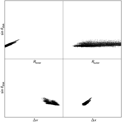
Figure 4: A plot of the correlations between the sine of the disk angle ($\sin\theta_{\mathrm{disk}}$) and the other accretion disk parameters for MRC0450-221: the inner disk radius ($R_{\mathrm{inner}}$), the outer disk radius ($R_{\mathrm{outer}}$), the local velocity dispersion of the disk material ($\Delta v$), and the shift of the disk emission with respect to 6564.61 Å ($\Delta x$). There are distributions for five different random seeds plotted here: for all seeds, the probability distributions converge on similar regions (but see discussion in Appendix A).

The disk angle has by far the greatest effect on the profile of the emission, since this parameter is most strongly correlated with the line width and the separation between the red and blue peaks of the line. The disk angle therefore constrains most strongly of all the disk fitting parameters, and so under the assumption of this given model, the double-peaked emission provides a reasonably robust method for measuring orientation. It should be emphasised that the model and input parameters chosen here (see Section 4.5) affect the range of disk emission profiles available during the fitting process, and hence may affect both the disk angles fitted and whether there is Bayesian evidence for a disk.

6 Results and Discussion

6.1 Fits to the emission spectra

The best-evidence Bayesian fits to the quasar spectra and the residuals from these fits are shown in Figure 5, where the fit is marked as a solid black line on the spectrum. In cases where disk models were selected, the disk component is shown by a dashed line, and the posterior distribution of the sine of the disk angle is shown in an inset plot. Each plot is labelled with the model with which it was fitted, and whether there is strong evidence for an accretion disk according to the Jeffreys’ criterion (SD), moderate evidence (MD), weak evidence (WD), whether the results are inconclusive but do not rule out a disk (PD), or whether there is strong evidence against the presence of a disk (ND) (see Table 6). Figure 6 shows the best-fit models from the subset which include a disk, for those quasars whose selected best-fit models do not include an accretion disk.

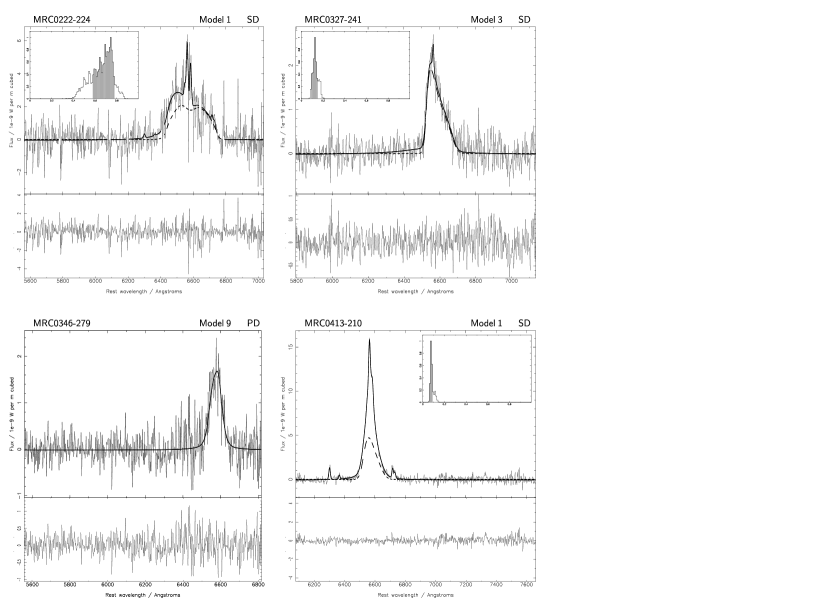
Figure 5: The best Bayesian fits to each quasar spectrum, and the residuals from the fit. The flux density scale of the residuals is the same as for the spectrum in most cases; for a few sources it is compressed, but the units remain the same. Wavelengths are rest-frame. The best fit is plotted as a solid black line. In cases where a disk is included in the selected model, the disk component is shown with a dashed line, and the posterior distribution of the sine of the disk angle is shown in an inset. In the inset plots, the y-axis shows the probability normalised to unity, and the x-axis covers the range $0<\sin{\theta}<1$. The shaded area of the inset plots shows the $1\sigma$ error bounds on the posterior distribution of the sine of the disk angle. Each plot is labelled with the index of the model with which it was fit, and with a code according to whether there is evidence for an accretion disk: SD = strong evidence for a disk; MD = moderate evidence for a disk; WD = weak evidence for a disk; PD = a possible disk (i.e. the evidence is inconclusive, or there is only weak or moderate evidence against the presence of a disk); ND = strong evidence against the presence of a disk.

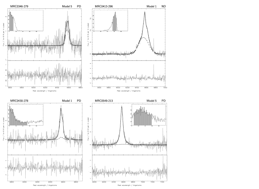
Figure 6: The best Bayesian fits which include an accretion disk component, for each quasar for which the highest evidence fit did not include a disk. Residuals are plotted below each fit. The flux density scale of the residuals is the same as for the spectrum in most cases; for a few sources it is compressed, but the units remain the same. Wavelengths are rest-frame. The best fit is plotted as a solid black line. The disk contribution is shown with a dashed line, and the posterior distribution of the sine of the disk angle is shown in an inset. In the inset plots, the y-axis shows the probability normalised to unity, and the x-axis covers the range $0<\sin{\theta}<1$. The shaded area of the inset plots shows the $1\sigma$ error bounds on the posterior distribution of the sine of the disk angle. Each plot is labelled with the index of the model with which it was fit, and with a code according to whether there is evidence for a disk: SD = strong evidence for a disk; MD = moderate evidence for a disk; WD = weak evidence for a disk; PD = a possible disk (i.e. the evidence is inconclusive, or there is only weak or moderate evidence against the presence of a disk); ND = strong evidence against the presence of a disk.

Table 7 summarises the results of the model selection process. Of the nineteen quasars, ten have strong evidence for disks according to Jeffreys’ criterion; two have weak evidence for a disk; six have possible disks, which means that either the results are inconclusive, or that there is weak or moderate evidence against a disk; and in only one case is there strong evidence against the presence of a disk.

The exceptional case, MRC0413-296, shows strong Bayesian evidence that there is no accretion disk emission in the spectrum. However, the best-fit model (Model 7, which includes the Lorentzian and Gaussian broad lines, in addition to both narrow H $\alpha$ and the forbidden narrow lines) did not fit in the expected manner: the width of the narrow H $\alpha$ emission was unconstrained in the fit, and this line was fitting to a third broad component. This quasar appears to be anomalous within the sub-sample in that two broad components are not sufficient to describe the emission, and therefore it is entirely plausible that this source requires a model not tested here, such as a three-component model including emission from an accretion disk, a BLR which gives rise to single-peaked lines, and an outflow.

It is very notable that for all but two sources (PD cases MRC0346-279 and MRC0549-213), the selected models include a complex BLR of more than one component. The most basic model of a single emitting region is not adequate to describe the complex profiles of the majority of these lines. In most of the cases, the preferred models were the ones with all the narrow lines and either the Lorentzian broad line plus the accretion disk (Model 1), or the Lorentzian line plus the broad Gaussian line (Model 7). In only four fits were models with less than the full complement of narrow lines preferred, and of these, three were spectra with low signal-to-noise ratios (MRC0327-241, MRC0346-279 and MRC1217-209). MRC0549-213 does appear to be well-fitted with a single broad Lorentzian line, with the possible presence of weak forbidden narrow lines, but very weak or absent narrow H $\alpha$.

None of the models with the accretion disk emission only were selected; in most cases, these models have extremely low evidence. There is certainly a component of the BLR which gives rise to single-peaked lines present.

The fitted posterior probability distributions for the sine of the disk angle, shown as insets in Figures 5 and 6, are on the whole reasonably well-constrained with slightly asymmetric distributions, though in some cases, these are cut off by the zero-angle prior boundary. MRC1019-227 has a double peak in the posterior probability distribution, though the two peaks are closely spaced. MRC1217-209 has a poorly-constrained distribution, due to the low signal-to-noise ratio of the spectrum. The MRC0430-278 spectrum has a low signal-to-noise ratio, and the fitted posterior probability distribution for the sine of the disk angle is therefore less tightly constrained in one region, although it is strongly peaked at low inclinations. MRC0549-213 has a posterior probability distribution for the sine of the disk angle which extends over the entire range. This source appears to have weak or absent disk emission, as it is well-fit by a Lorentzian line, but is classed as a PD source, as there is no strong evidence against a disk.

		Best-fit	Evidence	For best-fit model		For best-fit model
Quasar		model	for disk	with disk		without disk		Disk angle
				$\Delta\ln E^{2}_{1\mathrm{d}}$	$\Delta\ln E^{\mathrm{n}}_{1\mathrm{d}}$	$\Delta\ln E^{2}_{1\mathrm{n}}$	$\Delta\ln E^{\mathrm{d}}_{1\mathrm{n}}$
1	MRC0222-224	1	SD	6.43	12.50			48 ${}^{\circ}\pm{}^{2}_{12}$
2	MRC0327-241	3	SD	0.36	5.48			7 ${}^{\circ}\pm{}^{1}_{2}$
3	MRC0346-279	9 (5)	PD			0.80	1.91	1 ${}^{\circ}\pm{}^{5}_{1}$
4	MRC0413-210	1	SD	6.30	–			4 ${}^{\circ}\pm{}^{1}_{1}$
5	MRC0413-296	7 (1)	ND			10.79	–	39 ${}^{\circ}\pm{}^{3}_{6}$
6	MRC0430-278	7 (1)	PD			1.40	2.17	1 ${}^{\circ}\pm{}^{31}_{1}$
7	MRC0437-244	1	SD	1.44	91.96			18 ${}^{\circ}\pm{}^{2}_{1}$
8	MRC0450-221	1	SD	7.74	40.07			13 ${}^{\circ}\pm{}^{1}_{1}$
9	MRC0549-213	6 (5)	PD			0.90	2.34	15 ${}^{\circ}\pm{}^{20}_{12}$
10	MRC1019-227	1	WD	2.48	–			9 ${}^{\circ}\pm{}^{1}_{4}$
11	MRC1114-220	1	SD	4.40	7.93			35 ${}^{\circ}\pm{}^{4}_{12}$
12	MRC1208-277	1	SD	28.41	34.83			15 ${}^{\circ}\pm{}^{1}_{3}$
13	MRC1217-209	5	WD	0.64	1.37			8 ${}^{\circ}\pm{}^{14}_{2}$
14	MRC1222-293	1	SD	10.84	–			4 ${}^{\circ}\pm{}^{3}_{1}$
15	MRC1301-251	7 (1)	PD			0.54	–	28 ${}^{\circ}\pm{}^{14}_{11}$
16	MRC1349-265	7 (1)	PD			2.50	–	4 ${}^{\circ}\pm{}^{2}_{3}$
17	MRC1355-215	7 (1)	PD			1.61	–	4 ${}^{\circ}\pm{}^{2}_{1}$
18	MRC1355-236	1	SD	6.93	–			10 ${}^{\circ}\pm{}^{2}_{2}$
19	MRC1359-281	1	SD	6.64	–			4 ${}^{\circ}\pm{}^{1}_{1}$

Table 7: Summary of the model fitting results. Columns 1 and 2: Quasar index and MRC name; Column 3: Index of the best-fit model. If the selected model does not include an accretion disk, the index of the highest-evidence model which includes an accretion disk is shown in brackets. Column 4: Indication of whether there is evidence for a disk according to the odds ratio, with codes as follows: SD = strong evidence for a disk; MD = moderate evidence for a disk; WD = weak evidence for a disk; PD = a possible disk, i.e. the best fit is a non-disk model, but there is only inconclusive, weak or moderate evidence for this; ND = strong evidence against the presence of a disk; Columns 5 and 6: Natural logarithmic evidence difference between the best-fit model, in cases where this includes an accretion disk, and the second best model (Column 5, $\Delta\ln E^{2}_{1\mathrm{d}}$), and in cases where the second best fit also includes a disk, between the best-fit model and the best-fit model without a disk (Column 6, $\Delta\ln E^{\mathrm{n}}_{1\mathrm{d}}$); Columns 7 and 8: Natural logarithmic evidence difference between the best-fit model, in cases where this does not include an accretion disk, and the second best model (Column 7, $\Delta\ln E^{2}_{1\mathrm{n}}$), and in cases where the second best fit also does not include a disk, between the best-fit model and the best-fit model with a disk (Column 8, $\Delta\ln E^{\mathrm{d}}_{1\mathrm{n}}$); Column 9: Best-fit angle of the disk and the error in degrees.

The disks have fitted rotation axis angles between 1^∘ and 48^∘ to the line of sight; this range is consistent with the definition of quasars as being objects viewed within the opening angle of a dusty torus, where the opening angle is dependent on source luminosity but is generally supposed to be roughly 45^∘ for radio-luminous AGN (Lawrence, 1991).

Those sources with disk rotation axes at small angles to the line of sight in general have less strong evidence for a disk. The reason for this is that when the disk axis is at a small angle to the line of sight, the disk emission is not distinctive and double-peaked, but instead, rather similar to a Gaussian profile (see Section 5.5). In these cases, there is little to distinguish the Lorentzian plus accretion disk model for the broad emission from the Lorentzian plus Gaussian model, except that the fit with the Gaussian has fewer parameters, and is therefore likely to have a smaller prior parameter space and hence be favoured by Occam’s Razor. It is only those fits to sources with greater disk angles, or those with very high signal-to-noise ratio spectra, that make it possible to detect disk emission with high probability.

Figure 7 shows the disk angles from all model fits for each quasar. In most cases, the angles are extremely stable. In cases where there are differences in the inferred angles, all angles from models within one Jeffreys’ criterion of the best fit are consistent with each other.

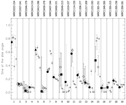
Figure 7: Disk angles for model fits with an accretion disk. Circular symbols indicate evidence for a disk, square symbols indicate a possible disk (inconclusive evidence, or weak to moderate evidence against a disk), while triangular symbols indicate strong evidence against the presence of a disk. White points mark fits which fall within one Jeffreys’ criterion of the best fit, and these can be seen in all cases to be consistent with the best-fit disk angle. The remainder of the fitted disk angles are plotted in pale grey.

6.2 Relationships with projected radio source size

The sine best-fit disk angles for the Molonglo quasars are plotted against the projected linear sizes of these sources in Figure 8. The source sizes are taken from Kapahi et al. (1998), or in some cases, new sizes were obtained from $\sim$ 1.4 GHz MERLIN radio maps (Down et al., in preparation): this data is summarised in Table 8. The sample can be divided into three source types on the basis of previous studies: core-dominated sources, Compact Steep Spectrum (CSS) sources, and non-CSS FRIIs. Two of the 19 sources are core-dominated, which are sources whose jets are oriented at small angles to the line of sight, and therefore have core-to-lobe radio flux density ratios of greater than unity; examination of their radio-frequency spectral energy distributions (Down et al., in preparation) reveals that these quasars have been boosted into this sample by virtue of their strong cores. The remainder of the sample is somewhat arbitrarily divided into six Compact Steep Spectrum sources, with projected sizes of less than 25 kpc (O’Dea, 1998) and 11 non-CSS FRII sources, with projected sizes of greater than 25 kpc.

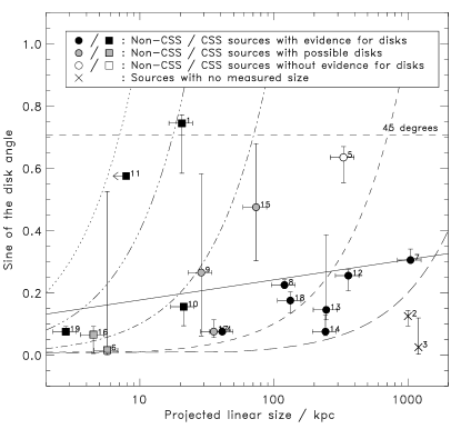
Figure 8: Sine best-fit disk angles versus the projected linear size of the quasar in kpc. The disk angle error bars include both the errors returned from the individual fits and a systematic error calculated from the variation in results from using different random seeds to initialise the Monte Carlo engines, added in quadrature, but do not take into account any error due to model selection. The non-CSS FRII sources are plotted with circles, and CSS sources are plotted with squares. The two sources plotted with crosses are core-dominated sources without measured projected sizes. The black points have weak to strong evidence for a disk, grey points have possible disks, and the white point has Bayesian evidence against the presence of a disk. Index numbers are matched to source names in Table 1. The black line shows the best linear fit to all sources excluding the core-dominated sources. There is a highly tentative correlation (Kendall $\tau$ coefficient of 0.40, significant at the $1\sigma$ level) between the sine of the disk angle and the projected linear size for all sources excluding the core-dominated sources, and for the 11 non-CSS FRII sources (Kendall $\tau$ coefficient of 0.44). The dotted, dot-dot-dot-dashed, dot-dashed, dashed and long-dashed lines show loci of constant deprojected size, for 10 kpc, 25 kpc, 100 kpc, 1 Mpc and 5 Mpc respectively.

There is a highly tentative correlation with a Kendall $\tau$ coefficient 0.44, probability of 65%, and significance of $<1\sigma$, calculated from ASURV (Lavalley et al., 1992), that for the eleven non-CSS FRII sources, the quasars with largest projected size have greater disk angles to the line of sight, as expected statistically from foreshortening if the accretion disk is perpendicular to the radio jet. The probability of a correlation is strengthened slightly to a Kendall $\tau$ coefficient of 0.40 with probability of 74% and $1\sigma$ significance if the six CSS sources are included in the sample. The weakness of the correlation is likely to be due to a large intrinsic scatter in the source size.

There are four CSS sources with fitted disk angles less than $10{}^{\circ}$ that appear to fall on the same relation as the non-CSS sources. It is probable that most or all of these are from the same population as the non-CSS sources, the only difference being projected size. The remaining two CSS sources, MRC0222-224 and MRC1114-220, have strong evidence for disks inclined at angles greater than $30{}^{\circ}$ to the line of sight.

The radio map for MRC0222-224 (see Kapahi et al. (1998)) shows two radio lobes with no hint of a core (a possible weak core is present between these lobes in a higher resolution MERLIN map, Down et al., in preparation); this quasar is consistent with an intrinsically small source viewed at a large angle to the accretion disk axis. The Balmer decrement for this quasar is estimated as H $\alpha$$/$ H $\beta$ $\sim$ 23, more than a factor of two higher than for any of the other sources in this Molonglo sub-sample (Janssens et al., in preparation). A simple interpretation is that this quasar is a young source, possibly surrounded by a cocoon of dust which reddens the optical emission (Baker et al., 2002).

The radio map of MRC1114-220 (de Silva et al., in preparation) reveals a strong radio core and single-sided jet, indicating that this source probably lies at a small angle to the line of sight, so that it is unlikely to be as intrinsically small as it appears. Possible explanations are that the accretion disk and radio jet are misaligned in this source following a merger event, or that the jet is precessing; however, this quasar merits further investigation.

The two quasars excluded from the sub-sample, MRC0418-288 and MRC1256-243, have small projected sizes. MRC0418-288 is a CSS source with projected size $D<16.6$ kpc, so is likely to be an intrinsically small, reddened source similar to MRC0222-224. MRC1256-243 has a larger size of $D\sim 65$ kpc and a high core-to-lobe flux density ratio at 10 GHz of $R_{10\mathrm{GHz}}\sim 3$, so is a core-dominated source: this is likely to have a small measured disk angle.

6.3 Deprojected source sizes

The source sizes were deprojected by dividing the apparent source sizes by the sine of the fitted disk angle, to compensate for simple geometric projection. This does not take into account the expansion of the source, but since the hotspots of jets are only expected to advance at $\sim 0.1$ c (Longair & Riley, 1979), this effect is small and is not considered. The deprojected sizes are given in Table 8, and are plotted in Figure 9.

			Proj.	Origin	Deproj.
Quasar		Type	source size	of	source
			$l$ (kpc)	$l$	size (kpc)
1	MRC0222-224	CSS	20.6	1	$28\pm^{8}_{1}$
2	MRC0327-241	CD	–		–
3	MRC0346-279	CD	–		–
4	MRC0413-210	FRII	41.2	2	$550\pm^{70}_{80}$
5	MRC0413-296	FRII	330.4	2	$520\pm^{80}_{30}$
6	MRC0430-278	CSS	5.7	1	$380\pm^{109000}_{370}$
7	MRC0437-244	FRII	1045.9	2	$3430\pm^{100}_{360}$
8	MRC0450-221	FRII	120.0	2	$530\pm^{30}_{40}$
9	MRC0549-213	FRII	28.7	2	$110\pm^{360}_{60}$
10	MRC1019-227	CSS	21.2	1	$140\pm^{90}_{10}$
11	MRC1114-220	CSS	$<$ 7.9	2	$<14\pm^{7}_{1}$
12	MRC1208-277	FRII	359.3	2	$1410\pm^{330}_{100}$
13	MRC1217-209	FRII	245.9	2	$1700\pm^{480}_{1060}$
14	MRC1222-293	FRII	242.7	2	$3240\pm^{660}_{1350}$
15	MRC1301-251	FRII	73.6	2	$160\pm^{90}_{50}$
16	MRC1349-265	CSS	4.5	1	$69\pm^{860}_{20}$
17	MRC1355-215	FRII	35.6	2	$480\pm^{160}_{160}$
18	MRC1355-236	FRII	132.6	2	$760\pm^{220}_{100}$
19	MRC1359-281	CSS	2.8	1	$37\pm^{5}_{7}$

Table 8: Summary of projected and deprojected source sizes. Columns 1 and 2: Quasar index and MRC name; Column 3: Source type – CD indicates sources with core-to-lobe radio flux ratio at 10 GHz of greater than 1, CSS indicates sources with $\alpha_{\mathrm{opt}}>0.5$ and projected source sizes $<$ 25 kpc, FRII indicates non-CSS FRII, which encompasses all other sources; Column 4: Projected source sizes in kpc; Column 5: Origin of projected source size measurement – 1 = New measurement (Down et al., in preparation), 2 = Kapahi et al. (1998); Column 6: Deprojected source sizes in kpc calculated using the fitted disk angles.

Figure 9: The solid line shows source sizes deprojected with the fitted disk angles (see Table 8). The projected sizes are plotted with a dotted line. Note that the two core-dominated sources have no measured size and are therefore excluded.

The distribution of deprojected source sizes found using the fitted disk angles is a single-peaked distribution, with the main concentration of sources in the range 100 kpc – 1 Mpc. Four of the CSS sources, MRC0222-224, MRC1114-220, MRC1349-265 and MRC1359-281, have deprojected sizes of less than 100 kpc. As the projected source sizes are defined as the distance between the centres of the furthest separated radio components (following de Silva et al. (in preparation)), the size may be underestimated if the whole source is not observed, i.e. in the case of MRC1114-220, only the core and approaching jet are visible, and so the size may be underestimated by a factor of $\sim 2$. There are hints that deprojection slightly tightens the distribution in source size as expected, but there is still a large scatter.

The cumulative distribution of the deprojected source sizes found using the best-fit disk angles is shown in Figure 10, with expected distributions of linear sizes, assuming that the hotspots of the lobes are expanding at a constant rate, shown for comparison. If the radio jet and accretion disk axes coincide, the calculated deprojected sizes are broadly consistent with a constant expansion of the heads of the jets up to $\sim 1$ Mpc, although there seems to be an excess of small sources. The distribution drops off at sizes greater than $\sim 1$ Mpc, which can be explained by the duty cycle of the quasars: the number of sources larger than a certain cut-off value will be depleted as they become quiescent (Bird et al., 2008). The distribution tails off more gradually than the highly simplified model, which can be explained by variation in hotspot advance speeds between quasars, some sources having an unusually long duty cycle, or by the largest sources being in especially low-density environments. The excluded sources, MRC0418-288 and MRC1256-243, are predicted to have very small and very large deprojected sizes respectively, so will not affect the overall distribution much.

Figure 10: Cumulative distribution of source sizes deprojected using the best-fit disk angles (solid line), with the projected source sizes shown for comparison (dotted line). The curves show the predicted distribution if the heads of the sources are expanding at a constant rate; the dot-dashed line is normalised at the deprojected size of the largest source in the sample, the dashed line is normalised at 1 Mpc. Note that the two core-dominated sources have no measured size, and are boosted into this sample by strong core emission, and are therefore excluded from this plot.

6.4 Relationships with radio luminosity

The sine of the best-fit disk angles are plotted against the 178 MHz radio luminosity in Figure 11. There is a correlation between these quantities, with a Kendall $\tau$ coefficient of 0.60, probability of 93% and $1.8\sigma$ significance. The measurement of the disk angle is entirely independent of the radio luminosity, so the fact that these parameters are correlated provides direct, albeit weak, evidence for the receding torus model (Lawrence, 1991), if the accretion disk axes align with the radio jets. According to this theory, sources with high radio luminosity have larger torus opening angles due to dust sublimation (Simpson, 1998), and therefore higher luminosity sources appear as quasars, rather than radio galaxies, up to a greater viewing angle (the critical angle). The prediction from this model is therefore that more luminous quasars have jet angles ranging up to a higher cut-off value, and if the disk angle is assumed to match the jet angle, the calculated disk angles support this prediction.

A calculation of the torus opening angle, following the model of Willott et al. (2000), normalised by a critical angle of $45{}^{\circ}$ at $\log L_{178\mathrm{MHz}}$= 27, and modified by a minimum quasar fraction of 10% which dominates the opening angle at low radio luminosities (e.g. Vardoulaki et al. (2008)), is also marked on Figure 11. The measured disk angles all fall within the calculated envelope of opening angles, and so assuming that the obscuring tori are aligned with the accretion disks, these results are in accordance with the receding torus model.

The missing source MRC1256-243 has luminosity $\log L_{178\mathrm{MHz}}\sim 27.4$, which is consistent with a low disk angle. MRC0418-288 has luminosity $\log L_{178\mathrm{MHz}}\sim 26.8$, which is a relatively low radio luminosity for the predicted large disk angle; however, an angle of $\sim 30{}^{\circ}$ would still be consistent with the receding torus scheme.

Figure 11: Sine best-fit disk angles versus logarithmic 178 MHz luminosity. The disk angle error bars include both the errors returned from the individual fits and a systematic error calculated from the variation in results from using different random seeds to initialise the Monte Carlo engines, added in quadrature, but do not take into account any error due to model selection. The non-CSS FRII sources and core-dominated sources are plotted as circles, and CSS sources are plotted as squares. The black points have weak to strong evidence for a disk, the grey points have possible disks (there is inconclusive evidence, or weak to moderate evidence against a disk) and the white points have strong evidence against a disk. Index numbers are matched to source names in Table 1. The best-fit line (minimising $\chi^{2}$) is shown in black. The dashed line shows the radio luminosity-dependent critical angle (following Willott et al. (2000)) with fiducial angle $45{}^{\circ}$ at $\log L_{178\mathrm{MHz}}$= 27, and minimum quasar fraction 10%.

6.5 Distribution of angles

The expected distribution of jet angles ($\theta$) can be modelled for the Molonglo quasar sample, including a Doppler-boosted core component. From Bayes’ Theorem

$$\mathrm{Prob}(\theta|L_{\mathrm{tot}}>L_{\mathrm{min}})\propto\mathrm{Prob}(L_{\mathrm{tot}}>L_{\mathrm{min}}|\theta)\times\mathrm{Prob}(\theta)$$ (8)

where $L_{\mathrm{tot}}$ is the total luminosity of the quasar and $L_{\mathrm{min}}$ is the limiting luminosity of the survey, and

$$\mathrm{Prob}(\theta)=2\pi\sin\theta\mathrm{d}\theta\,\,.$$ (9)

The proportionality is required because there is no solid information about the overall number of sources for which $L_{\mathrm{tot}}>L_{\mathrm{min}}$.

Marginalising the lobe luminosity, then

$$\mathrm{Prob}(L_{\mathrm{tot}}>L_{\mathrm{min}}|\theta) \propto \int_{0}^{\infty}\mathrm{Prob}(L_{\mathrm{tot}}>L_{\mathrm{min}}|\theta,L_{\mathrm{lobe}})$$ (10)

$$\times\mathrm{Prob}(L_{\mathrm{lobe}})\mathrm{d}L_{\mathrm{lobe}}\,\,.$$

From Willott et al. (2001), the radio luminosity function of high luminosity AGN is

$$\rho(L)=\rho_{\mathrm{norm}}\Big{(}\frac{L}{L_{\mathrm{norm}}}\Big{)}^{-\alpha},$$ (11)

where $\rho$ is the comoving space density of sources in logarithmic luminosity space and $\alpha\sim 2.3$. Since this relation was found for luminosities of 151 MHz and 178 MHz, then the total luminosity is low enough in frequency to be approximated as the lobe luminosity. Then

$$\mathrm{Prob}(L_{\mathrm{lobe}}) \propto L_{\mathrm{lobe}}^{-\alpha}\times\frac{\mathrm{d}\log L_{\mathrm{lobe}}}{L_{\mathrm{lobe}}}$$ (12)

$$\propto L_{\mathrm{lobe}}^{-\alpha-1}\,\,.$$

Defining the core-to-lobe flux ratio $R$ in the same way as Jackson & Wall (1999), then

$$R=R_{c}\frac{1}{\gamma^{2}}\left(\frac{1}{(1+\beta\cos\theta)^{2}}+\frac{1}{(1-\beta\cos\theta)^{2}}\right)\,\,,$$ (13)

where $R_{c}$ is some fiducial value of $R$, and is found by Jackson & Wall (1999) to be $R_{c}\sim 0.01$ for FRII sources; $\gamma$ is the Lorentz factor and $\beta$ is the velocity of the jet in units of c. The total flux density, $S_{\mathrm{tot}}$, is then defined as

$$S_{\mathrm{tot}}=S_{\mathrm{lobe}}(1+R)\,\,,$$ (14)

and since flux density is proportional to luminosity, then

$$L_{\mathrm{tot}}=L_{\mathrm{lobe}}(1+R)\,\,.$$ (15)

Now for each value of $L_{\mathrm{lobe}}$ and $\theta$, the total luminosity is uniquely defined, and $\mathrm{Prob}(L_{\mathrm{tot}}>L_{\mathrm{min}}|\theta,L_{\mathrm{lobe}})$ becomes simply 0 or 1. The outcome of this is that for a given $\theta$, there is one limiting lobe flux $L_{\mathrm{lim}}(\theta)$ above which the probability of detecting a source is unity, and below which it is zero, and this simply changes the limits on the integration so that, substituting equations (9), (10) and (12) into equation (8) we find

$$\mathrm{Prob}(\theta|L_{\mathrm{tot}}>L_{\mathrm{min}})\propto\int_{L_{\mathrm{lim}}(\theta)}^{\infty}L_{\mathrm{lobe}}^{-\alpha-1}\mathrm{d}L_{\mathrm{lobe}}\times\sin\theta\mathrm{d}\theta\,\,.$$ (16)

This integrates to

$$\mathrm{Prob}(\theta|L_{\mathrm{tot}}>L_{\mathrm{min}}) \propto [-L_{\mathrm{lobe}}^{-\alpha}]_{L_{\mathrm{lim}}(\theta)}^{\infty}\times\sin\theta$$ (17)

$$\propto L_{\mathrm{lim}}(\theta)^{-\alpha}\times\sin\theta\,\,.$$

Figure 12 shows the cumulative probability distribution for the disk angles, together with the theoretical distributions of jet angle for different values of the Lorentz factor $\gamma$. If the accretion disk axis and radio jets align (i.e. if the disk is perpendicular to the jet), then the distribution of disk angles is most consistent with a value of the jet Lorentz factor around $\gamma\sim 20$. It should be noted that MRC0418-288 was excluded from this sub-sample of quasars on the basis of optical faintness. This source has a high probability of being at a large angle to the line of sight, since it may well be a reddened source in which the dusty torus is blocking some sight lines to the optically bright nucleus (e.g. Baker et al. (2002)). MRC1256-243 is a core-dominated source, which is likely to have a very small disk angle. An extra quasar added to the each end of the disk angle distribution function would make it more in agreement with the modelled angular distribution for $\gamma=20$.

This Lorentz factor differs from the $\gamma\sim 3$ measured from the 3C sample. This is explicable if $\gamma$ is dependent on angle, such that $\gamma\sim 20$ close to the line of sight, when viewing the quasars down the axes of their jets, and $\gamma\sim 3$ when viewed at larger angles (e.g. Hardcastle (2006)). The angular distribution of the Molonglo quasars, which are selected at intermediate radio frequency, is dominated by Doppler boosting, whereas this is a small effect for the 3CRR sample. The distribution of the fitted Lorentz factor for the 3CRR sample is centred around $\gamma\sim 3$, though with a slight asymmetry biased towards higher values of $\gamma$, whereas the Molonglo sample is predicted to have more probability of higher $\gamma$ factors. It is not sufficient to model the jet with a single Lorentz factor. The luminosity – jet angle relation is also expected to have some scatter in $\gamma$ due to intrinsic differences in the sources.

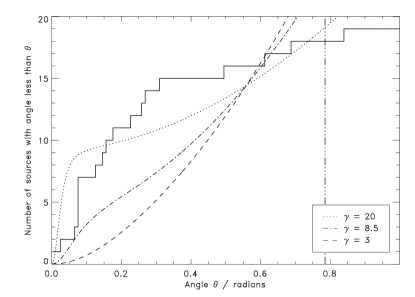
Figure 12: The cumulative distribution of the best-fit disk angles (solid black line). The curves show the theoretical distributions of jet angle, modelled from the Jackson & Wall (1999) relation and normalised up to an angle of $45{}^{\circ}$, for different values of the Lorentz factor: the dashed line shows the expected cumulative distribution for $\gamma=3$, the dot-dashed line for $\gamma=8.5$, and the dotted line for $\gamma=20$. The vertical dot-dot-dot-dashed line indicates a disk angle of $45{}^{\circ}$.

The distribution in fitted disk angle levels off at $48{}^{\circ}$. This is consistent with the opening angle which might be expected for a sample of powerful FRII sources. The fact that no quasars are observed with disk angles larger than $48{}^{\circ}$ adds to the evidence for the unification scheme which suggests radio galaxies and quasars are the same objects viewed at decreasing angles to the line of sight.

6.6 Velocity shifts

6.6.1 Velocity shift measurements

The prior ranges on the positions of the single-peaked broad line components allowed shifts of $\Delta z=\pm 0.015$ compared to the fitted positions of the narrow lines, corresponding to line shifts of $\sim 4500$ km s^-1. If no narrow lines were fitted, the shift of the Gaussian line was measured relative to the Lorentzian line. The accretion disk was allowed to shift to a similar degree, $\Delta\lambda=\pm 100$ Å with respect to the laboratory wavelength. The fitted velocity shifts from the best-fit models are given in Table 9.

		For best-fit model including disk:			For best-fit model without disk:
Quasar			$\Delta v_{\mathrm{disk}}$	$\Delta v_{\mathrm{Lorentzian}}$		$\Delta v_{\mathrm{Lorentzian}}$	$\Delta v_{\mathrm{Gaussian}}$
		Model	(km s-1)	(km s-1)	Model	(km s-1)	(km s-1)
(1)	(2)	(3)	(4)	(5)	(6)	(7)	(8)
1	MRC0222-224	1	750 $\pm{}^{690}_{250}$	-4460 $\pm{}^{40}_{740}$
2	MRC0327-241	3	-830 $\pm{}^{230}_{740}$	-3920 $\pm{}^{580}_{2750}$
3	MRC0346-279	5	-1100 $\pm{}^{850}_{290}$ ∗	–	9	–	1570 $\pm{}^{2400}_{220}$ †
4	MRC0413-210	1	-1490 $\pm{}^{380}_{340}$	310 $\pm{}^{20}_{100}$
5	MRC0413-296	1	-350 $\pm{}^{140}_{150}$	2750 $\pm{}^{110}_{90}$	7	2930 $\pm{}^{90}_{80}$	-140 $\pm{}^{110}_{70}$
6	MRC0430-278	1	-1350 $\pm{}^{1130}_{3330}$	-400 $\pm{}^{100}_{120}$	7	400 $\pm{}^{120}_{190}$	-1490 $\pm{}^{140}_{2250}$
7	MRC0437-244	1	-2660 $\pm{}^{90}_{500}$	410 $\pm{}^{30}_{50}$
8	MRC0450-221	1	-1330 $\pm{}^{170}_{330}$	-490 $\pm{}^{300}_{200}$
9	MRC0549-213	5	2160 $\pm{}^{2690}_{1600}$ ∗	–
10	MRC1019-227	1	340 $\pm{}^{610}_{170}$	220 $\pm{}^{100}_{130}$
11	MRC1114-220	1	1780 $\pm{}^{410}_{280}$	220 $\pm{}^{90}_{40}$
12	MRC1208-277	1	-1740 $\pm{}^{520}_{200}$	-1220 $\pm{}^{60}_{40}$
13	MRC1217-209	5	900 $\pm{}^{1050}_{1820}$ ∗	–
14	MRC1222-293	1	-1650 $\pm{}^{550}_{570}$	-230 $\pm{}^{40}_{90}$
15	MRC1301-251	1	400 $\pm{}^{690}_{320}$	-4460 $\pm{}^{40}_{3610}$	7	-4190 $\pm{}^{190}_{110}$	4460 $\pm{}^{330}_{40}$
16	MRC1349-265	1	640 $\pm{}^{630}_{240}$	40 $\pm{}^{100}_{250}$	7	40 $\pm{}^{140}_{130}$	1040 $\pm{}^{120}_{110}$
17	MRC1355-215	1	1620 $\pm{}^{890}_{270}$	-310 $\pm{}^{60}_{110}$	7	-310 $\pm{}^{90}_{40}$	1670 $\pm{}^{290}_{190}$
18	MRC1355-236	1	310 $\pm{}^{60}_{560}$	-1940 $\pm{}^{270}_{80}$
19	MRC1359-281	1	-830 $\pm{}^{280}_{580}$	-590 $\pm{}^{180}_{90}$

Table 9: Velocity shifts of the broad line components. Columns 1 and 2: Quasar index and MRC name; Column 3: Best-fit disk model; Column 4: Disk emission shift relative to narrow H $\alpha$ in km s^-1 for the best-fit disk model; Column 5: Lorentzian line shift relative to narrow H $\alpha$ in km s^-1 for the best-fit disk model; Column 6: Best-fit model in cases where this does not include a disk; Column 7: Broad Lorentzian shift relative to narrow H $\alpha$ in km s^-1, for the best-fit model in cases where this does not include a disk; Column 8: Broad Gaussian shift relative to narrow H $\alpha$ in km s^-1, for the best-fit model in cases where this does not include a disk. ^∗ No narrow H $\alpha$ was fitted in this model, and so the shift of the disk emission relative to the broad Lorentzian is given in km s^-1. ^† No narrow H $\alpha$ was fitted in this model, and so the shift of the broad Gaussian relative to the broad Lorentzian is given in km s^-1.

In seven cases, the measured velocity shifts cannot be trusted. This occurs in cases where the fitted parameters of either the broad Lorentzian line or narrow H $\alpha$ are not constrained by the prior range. There are four potential reasons for this. (1) The velocity shift of the broad Lorentzian is unconstrained by the fit; this component is fitting to a broadband bump in the continuum left by imperfect continuum subtraction, rather than to the emission line profile, so this fitted value is not correct. This affects the quasars MRC0327-224 and MRC1301-251. (2) The broad Lorentzian is clearly fitting to an additional narrow line component, and has unconstrained width as a result. This affects MRC1208-277. (3) Narrow H $\alpha$ is fitting to an extra broad component, and therefore the fitted position of this line is not reliable. The relative shifts of the broad components to each other will be of the right magnitude so long as the extra broad component fitted by narrow H $\alpha$ is small. This affects MRC0413-296, MRC0430-278 and MRC1222-293. (4) In the case of MRC0222-224, there is some degeneracy in the fit of the broad Lorentzian, such that the shift of this line is not properly constrained.

6.6.2 Discussion of the velocity shifts

Figure 13 shows the shifts of the broad emission components for the best-fit models which include an accretion disk. Note that these models all include a Lorentzian line in addition to the disk emission. Three of the sources were best fitted with models which did not include narrow lines, and hence do not have shifts measured relative to the NLR; none of these quasars have published redshifts from high-resolution observations of narrow lines, so these were excluded. The distribution of fitted disk shifts is relatively evenly distributed between -2000 km s^-1 and +2000 km s^-1, with the exception of MRC0437-244 with a disk shift of -2660 km s^-1 relative to the narrow lines. This distribution does not change significantly if only the reliable shifts are considered.

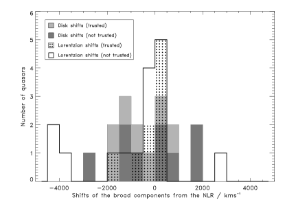
Figure 13: Distribution of line shifts for the best-fit models which include an accretion disk. The disk shifts with respect to narrow H $\alpha$ are shown as a grey-shaded histogram, and the Lorentzian line shifts with respect to narrow H $\alpha$ are shown as a solid-line histogram. The subsets of these with reliable measurements are marked with dark-grey shading and dot shading respectively. Note that three sources are excluded as no narrow lines were fit for these spectra.

The fitted Lorentzian line shifts are distributed in three groups. The largest group have relatively modest velocity offsets to the NLR, with 9/16 shifts within $\pm 500$ km s^-1 of the narrow line position, and a small tail out to -2000 km s^-1. There is one source only with a Lorentzian line shift relative to the narrow lines of more than +500 km s^-1: MRC0413-296 has a fitted shift of +2750 km s^-1, but this is not reliable, since the narrow lines were fitting to an extra broad component in this spectrum and hence the H $\alpha$ line centre used for reference was not reliably fitted. There are also three sources with blueshifts of -3500 – -4500 km s^-1. Of these three quasars, two have Lorentzian lines which are fitting to a component of the continuum rather than the broad H $\alpha$ emission, and the other has degeneracy in the fitted values of the Lorentzian line, so the shifts for these sources are not trustworthy. Therefore, all dependable Lorentzian line shifts fall in the central group, with moderate redshifts with respect to the NLR, or moderate to high blueshifts with respect to the NLR.

Table 10 gives the average shifts of the broad line components and their standard errors. The spread of shifts is very wide, but when only the reliable velocity shifts are considered, both the accretion disk and the Lorentzian line have average blueshifts of order -200 km s^-1. Taken overall, there is a trend within this sample of powerful quasars for the broad emission to be blueshifted, in agreement with the majority of the literature (see Section 1.3). It should be borne in mind that the outflows and inflows may be symmetric, but if dust in the plane of the accretion disk obscures the far-side emission from view, the shifts measured are for the near-side quasar emission.

Separating the sample into 10 low-$z$ ($z<1$) and 6 high-$z$ ($z>1.5$) sources and considering only the trustworthy shifts (6 and 3 sources respectively for low-$z$ and high-$z$), the average Lorentzian line shift is -380 km s^-1 for the low-$z$ sources and +40 km s^-1 for the high-$z$ sources, consistent with this emission originating close to the systemic velocity. The average accretion disk shift for the trustworthy sources is -890 km s^-1 for the low-$z$ sources and +620 km s^-1 for the high-$z$ sources, so the disk emission is blueshifted with respect to systemic velocity at low-$z$ and redshifted at high-$z$.

	All shifts			Trusted shifts only
Source of emission	Average shift	Standard error	No. of sources	Average shift	Standard error	No. of sources
(and $z$ range)	(km s-1)	(km s-1)		(km s-1)	(km s-1)
Accretion disk (all)	-400	310	16	-180	470	9
Accretion disk (low-$z$)	-920	320	10	-890	460	6
Accretion disk (high-$z$)	460	440	6	620	260	3
Lorentzian line (all)	-880	470	16	-240	230	9
Lorentzian line (low-$z$)	-1210	520	10	-380	320	6
Lorentzian shift (high-$z$)	-330	890	6	40	150	3

Table 10: Summary of the mean averages and standard errors of the shifts of the broad emission components, for best-fit models which include an accretion disk. Shifts are given for both the entire sample, and only those sources whose shifts are reliable; and are given for sub-samples divided by redshift: the sample as a whole, the low-$z$ fraction ($z<1$), and the high-$z$ fraction ($z>1.5$). The number of sources in each sub-sample is shown.

Figure 14 shows the broad-line velocity shifts from the best-fit disk models plotted against quasar redshift. The redshift and the shift of the accretion disk emission with respect to the narrow lines are correlated with a Kendall $\tau$ coefficient of 0.850, significant at the $2\sigma$ level (98% probability of a correlation). This correlation may arise from the dependence of both these quantities on optical luminosity (Wills, 1980) or radio luminosity. The relation between AGN redshift and luminosity is well-known, and occurs because sources at greater distances are more powerful. This effect, the Malmquist Bias, is illustrated in Table 11, which shows that the sources with $z>1.5$ are more luminous than the $z<1$ sources at radio frequencies, and in terms of optical continuum and emission lines. There is no correlation apparent between the quasar redshift and the shift of the fitted Lorentzian line with respect to the narrow lines, with a Kendall $\tau$ of 0.133 (significance of $<0.5\sigma$, 28% probability of a correlation). It appears that the shifts between the single-peaked broad emission line and the NLR are modest.

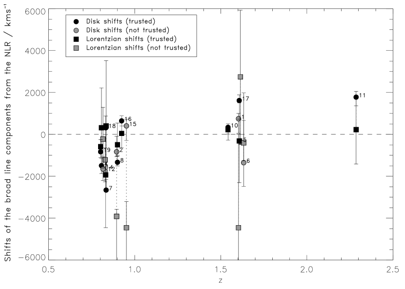
Figure 14: Accretion disk shifts (circles) and Lorentzian line shifts (squares) with respect to narrow H $\alpha$ for the best-fit models which include a disk, plotted against the source redshift. Black points indicate sources in which the shifts are reliable, and grey points indicate sources in which the shifts are not trusted (see Section 6.6.1). Dotted lines join the disk and Lorentzian shifts from the same source, where the error bars do not overlap. The lower limits of the error bars for sources 2, 15 and 1 which are not shown on the plot are -9700 km s^-1, -7600 km s^-1 and -9400 km s^-1 respectively.

	$z<1$		$z>1.5$		All $z$
	Av.	Err.	Av.	Err.	Av.	Err.
$L_{151\mathrm{MHz}}$	26.9	0.1	27.8	0.1	27.3	0.1
$b_{\mathrm{J}}$	-24.8	0.3	-25.7	0.4	-25.1	0.3
$L_{\mathrm{Nar}\,H_{\alpha}}$	0.135	0.030	0.541	0.221	0.285	0.095
$L_{\mathrm{Brd}\,H_{\alpha}}$	3.93	1.05	19.54	6.49	9.69	3.02

Table 11: Average luminosities for the quasar sub-sample divided by redshift into a low-$z$ fraction ($z<1$), and a high-$z$ fraction ($z>1.5$), and for the combined sample. Row 1: Logarithmic 151 MHz luminosity; Row 2: Optical $b_{\mathrm{J}}$ magnitudes from the UK Schmidt IIaJ plates, where $b_{\mathrm{J}}=B-0.23(B-V)$ (Bahcall & Soneira, 1980); Row 3: Luminosities of the narrow H $\alpha$ lines in units of 10³⁶ W sr^-1; Row 4: Luminosities of the broad H $\alpha$ lines in units of 10³⁶ W sr^-1.

Large-scale emission is most commonly seen alongside the radio jets or within the ionisation cone of the source, e.g. Nesvadba et al. (2008). If it is the case that the material flows alongside the jet, the greatest velocity shifts should be observed for sources at small angles to the line of sight. No correlation is found between the magnitude of the velocity shift of the disk with respect to the NLR and the sine of the disk angle to the line of sight (Kendall $\tau$ coefficient -0.05, significance of $<0.1\sigma$, probability of correlation 11%); the velocity shifts are plotted against the disk angle in Figure 15. However, the sources at $\gtrsim 30{}^{\circ}$ show velocity shifts of less than $\pm 1000$ km s^-1 (note that these are not reliable shifts), with the exception of MRC1114-220, which is a young radio source, and hence is more likely to have a misaligned disk. The narrow line gas may in fact be entrained along the jet, but moving in a transverse direction: Nesvadba et al. (2006) and Nesvadba et al. (2008) suggest from integral field studies of a small sample of high-redshift radio galaxies that the ionised gas is being accelerated away from the nucleus of the galaxy by expanding cocoons of hot gas around the jets. There are also indications that the distribution of gas surrounding CSS sources does not mirror that seen in the larger sources, with more dust and gas seen in edge-on CSS sources, and so it is probable that the velocity distribution of the material in these young sources will also differ.

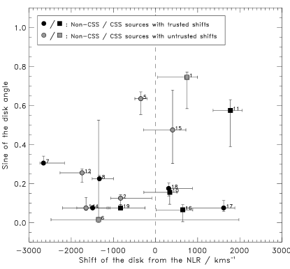
Figure 15: Best-fit accretion disk angle plotted against the shift of the disk emission with respect to narrow H $\alpha$ for non-CSS sources (circles) and CSS sources (squares). The points with reliable shifts are plotted in black; those sources whose shifts are not trusted are plotted in grey.

There is no evidence for a correlation between the magnitude of the disk shift with respect to the NLR and the width of the narrow lines (deconvolved from instrumental effects), with Kendall $\tau$ of -0.283, significance $<1\sigma$, a probability for anticorrelation of 56%. The narrow lines would be expected to have broader profiles for greater velocity shifts if the shift between the disk emission and the narrow line emission is due to the narrow lines forming in a moving mass of gas.

The measured velocity shifts for the broad components relative to the narrow lines imply that the single-peaked broad lines arise from a region with a similar velocity to the NLR, while the disk is redshifted relative to these regions for higher-$z$, and hence brighter, sources, and blueshifted in relation to these for lower-$z$ sources. The accretion disk is expected to be fixed at the systemic redshift, and therefore these results can be interpreted as the single-peaked broad lines and narrow lines arising from outflowing material in optically-luminous sources, and infalling material in less luminous sources. This could be the result of a quasar wind model of AGN feedback, in which powerful quasars fuel outflows which sweep the gas out of the galaxy (Silk & Rees, 1998); the outflows are expected to scale with the quasar luminosity.

7 Effects of Model Assumptions

7.1 Models with the NLR and accretion disk fixed at the same redshift

If the narrow lines are formed at the systemic redshift, as much of the literature indicates, then there should be minimal velocity shift between the accretion disk and the NLR. In order to test the effect of this alternative assumption, a second set of models was fitted, with the disk emission fixed at the same redshift as the narrow lines. Aside from the exclusion of one parameter describing the shift between these two emission components, the models are identical, and in the cases of the models with no narrow lines, the disk is allowed to shift as usual; this change therefore affects only four models (1, 3, 10 and 11).

7.2 Notes on individual quasars

MRC0222-224: Model 1 was selected with higher evidence by $\Delta\ln(\mathrm{Evidence})=6.0$ than Model 10, the next best model.

MRC0327-241: The best-fit model is Model 1. Models 3, 5 and 10 are also within the $\Delta\ln(\mathrm{Evidence})=5$ bound of this model; however, all these models include disk emission, so this quasar has strong evidence for a disk.

MRC0346-279: This low signal-to-noise spectrum does not differentiate well between the models. Model 9 was selected by the Bayesian evidence, with higher evidence by $\Delta\ln(\mathrm{Evidence})=0.80$ over the next best fit.

MRC0413-210: Model 1 was selected, with $\Delta\ln(\mathrm{Evidence})=7.7$ over the next best model.

MRC0413-296: As before, although the spectrum of this quasar clearly contains narrow lines, the narrow line parameters instead fitted broad components of emission. The best model is Model 7, with evidence over the next best-fit model of $\Delta\ln(\mathrm{Evidence})=12.1$. This quasar has strong evidence against the presence of a disk.

MRC0430-278: The preferred model for this spectrum is Model 7, though many models fall within the Jeffreys’ criterion. The margin in logarithmic evidence of Model 7 over Model 3, the best-fit model which includes disk emission, is only $\Delta\ln(\mathrm{Evidence})=2.3$, so this is a “possible disk” quasar.

MRC0437-244: Model 5, including a disk, was selected with strong evidence.

MRC0450-221: Model 1, including a disk, was selected with strong evidence. The fitted disk angle is not within the errors of the fitted angle from the first analysis: 20${}^{\circ}\pm{}^{1}_{1}$ from this analysis compared to 13${}^{\circ}\pm{}^{1}_{1}$ for the case in which the accretion disk is allowed to shift.

MRC0549-213: Many of the models fall within the Jeffreys’ criterion of the best-fit model, including three of the disk models, so this quasar is a “possible disk” source. The selected model was Model 6, but this is preferred over the best-fit disk model, Model 1, by only $\Delta\ln(\mathrm{Evidence})=1.7$.

MRC1019-227: Model 1 is preferred by only $\Delta\ln(\mathrm{Evidence})=1.5$ over Model 7, so this source has a “weak disk” classification.

MRC1114-220: Model 1 was selected by $\Delta\ln(\mathrm{Evidence})=6.3$ over Model 7, the best-fit model without a disk, so there is strong evidence for a disk. The fitted angle, 15${}^{\circ}\pm{}^{1}_{4}$, is not in agreement with the angle found from the analysis in which the disk is allowed to shift with respect to the narrow lines (35${}^{\circ}\pm{}^{4}_{12}$).

MRC1208-277: Model 7 was selected with evidence difference $\Delta\ln(\mathrm{Evidence})=86.3$ over Model 3, which contains a disk, so this has strong evidence against a disk. The fitted angle is 46${}^{\circ}\pm{}^{4}_{3}$, which is strongly in disagreement with the case in which the disk is allowed to shift with respect to the NLR (15${}^{\circ}\pm{}^{1}_{3}$).

MRC1217-209: Model 5 was selected, but many of the models fall within the Jeffreys’ criterion of this model. There is an evidence difference between Model 5 and Model 9, the best-fit model without a disk, of $\Delta\ln(\mathrm{Evidence})=1.4$.

MRC1222-293: Model 7 was selected as the best-fit model, with evidence difference of $\Delta\ln(\mathrm{Evidence})=50.4$ over Model 1, which is the highest-evidence model including an accretion disk. The fitted angle is 19${}^{\circ}\pm{}^{1}_{3}$, which is in disagreement with the angle found from the analysis is which the disk is allowed a velocity shift with respect to the NLR (4${}^{\circ}\pm{}^{3}_{1}$).

MRC1301-251: Model 7 is preferred by a margin of $\Delta\ln(\mathrm{Evidence})=0.05$ over Model 10, the highest-evidence model including a disk, and by a margin of $\Delta\ln(\mathrm{Evidence})=0.8$ over Model 1, so any of these models are plausible.

MRC1349-265: Model 7 was selected by $\Delta\ln(\mathrm{Evidence})=1.9$ over Model 1, the highest-evidence model including a disk.

MRC1355-215: Model 7 was selected over the next best model, Model 1, by $\Delta\ln(\mathrm{Evidence})=3.7$.

MRC1355-236: Model 1 was selected with strong evidence.

MRC1359-281: There is strong evidence for Model 1. The fitted angle is 7${}^{\circ}\pm{}^{1}_{1}$, which does not agree with the angle fitted from the first analysis, 4${}^{\circ}\pm{}^{1}_{1}$, for the case in which the accretion disk is not fixed at the redshift of the narrow lines.

7.3 Fits to the emission spectra

Table 12 gives the results of the model selection for the case in which the NLR and the accretion disk are fixed at the same redshift. For 14 out of 19 sources, the $1\sigma$ error range of the best-fit disk angle from the new analysis overlaps with the $1\sigma$ error range of the best-fit disk angle for the case in which the disk is allowed to shift with respect to the NLR. The remaining five are MRC0450-221, MRC1114-220, MRC1208-277, MRC1222-293 and MRC1359-281.

The narrow line centres of a number of the models were not strongly constrained in the fitting process, and since the disk and NLR are fixed at the same redshift in this regime, an incorrectly fitted narrow line centre leads to an offset in the disk position as well, giving an erroneous fitted angle. This potentially affects MRC0327-241 (in which the narrow line position differed by 20Å between the fit from the analysis in which the disk shift is allowed and the one in which it is not); MRC1114-220, in which there was degeneracy in the fitted position of the narrow H $\alpha$; MRC0413-296, MRC0430-278, MRC1222-293 and MRC1359-281, in which the narrow lines were fit with very broad widths ($\gtrsim$ 30 Å), and hence their positions may not have been fixed to very good accuracy. This effect might plausibly be the reason that the disk angles from the two analyses do not agree for MRC1114-220 and MRC1359-281. However, at least MRC0450-221, MRC1208-277 and MRC1222-293 have different disk angles as a direct result of the fixing of the accretion disk at the redshift of the NLR.

In addition to the inconsistency in disk angles for these five sources between the two analyses, the two sources with the most extreme changes in fitted disk angle (MRC1208-277 and MRC1222-293) have changed from having strong Bayesian evidence in favour of a disk, in the regime where a disk shift is allowed from the NLR, to having strong Bayesian evidence against the presence of disk, when the disk is fixed at the redshift of the NLR. The volume of prior parameter space was reduced in this second analysis by the removal of a variable, which, if this variable was extraneous, would have increased the Bayesian evidence for the presence of accretion disks. The fact that the evidence remained similar in the majority of cases, but declined sharply in these two cases, implies that the variable describing the velocity shift between the disk and the NLR is required.

		Best-fit	Evidence	For best-fit model		For best-fit model			Analysis with disk shift allowed
Quasar		model	for disk	with disk		without disk		Disk	Best-fit	Evidence	Disk
				$\Delta\ln E^{2}_{1\mathrm{d}}$	$\Delta\ln E^{\mathrm{n}}_{1\mathrm{d}}$	$\Delta\ln E^{2}_{1\mathrm{n}}$	$\Delta\ln E^{\mathrm{d}}_{1\mathrm{n}}$	angle	Model	for disk	angle
1	MRC0222-224	1	SD	6.02	11.71			53${}^{\circ}\pm{}^{7}_{11}$	1	SD	48 ${}^{\circ}\pm{}^{2}_{12}$
2	MRC0327-241	1	SD	1.77	7.06			7${}^{\circ}\pm{}^{1}_{1}$	3	SD	7 ${}^{\circ}\pm{}^{1}_{2}$
3	MRC0346-279	9 (1)	PD			0.80	1.08	10${}^{\circ}\pm{}^{3}_{5}$	9 (5)	PD	1 ${}^{\circ}\pm{}^{5}_{1}$
4	MRC0413-210	1	SD	7.66	–			9${}^{\circ}\pm{}^{3}_{4}$	1	SD	4 ${}^{\circ}\pm{}^{1}_{1}$
5	MRC0413-296	7 (1)	ND			12.12	–	42${}^{\circ}\pm{}^{2}_{2}$	7 (1)	ND	39 ${}^{\circ}\pm{}^{3}_{6}$
6	MRC0430-278	7 (3)	PD			1.40	2.05	8${}^{\circ}\pm{}^{3}_{4}$	7 (1)	PD	1 ${}^{\circ}\pm{}^{31}_{1}$
7	MRC0437-244	5	SD	16.87	62.52			21${}^{\circ}\pm{}^{1}_{1}$	1	SD	18 ${}^{\circ}\pm{}^{2}_{1}$
8	MRC0450-221	1	SD	8.06	39.27			20${}^{\circ}\pm{}^{1}_{1}$	1	SD	13 ${}^{\circ}\pm{}^{1}_{1}$
9	MRC0549-213	6 (1)	PD			0.90	1.70	7${}^{\circ}\pm{}^{17}_{6}$	6 (5)	PD	15 ${}^{\circ}\pm{}^{20}_{12}$
10	MRC1019-227	1	WD	1.53	–			6${}^{\circ}\pm{}^{1}_{1}$	1	WD	9 ${}^{\circ}\pm{}^{1}_{4}$
11	MRC1114-220	1	SD	4.14	6.25			15${}^{\circ}\pm{}^{1}_{4}$	1	SD	35 ${}^{\circ}\pm{}^{4}_{12}$
12	MRC1208-277	7 (3)	ND			86.26	–	46${}^{\circ}\pm{}^{4}_{3}$	1	SD	15 ${}^{\circ}\pm{}^{1}_{3}$
13	MRC1217-209	5	WD	1.37	–			8${}^{\circ}\pm{}^{14}_{2}$	5	WD	8 ${}^{\circ}\pm{}^{14}_{2}$
14	MRC1222-293	7 (1)	ND			26.92	50.36	19${}^{\circ}\pm{}^{1}_{3}$	1	SD	4 ${}^{\circ}\pm{}^{3}_{1}$
15	MRC1301-251	7 (10)	PD			0.05	–	31${}^{\circ}\pm{}^{2}_{2}$	7 (1)	PD	28 ${}^{\circ}\pm{}^{14}_{11}$
16	MRC1349-265	7 (1)	PD			1.94	–	4${}^{\circ}\pm{}^{1}_{3}$	7 (1)	PD	4 ${}^{\circ}\pm{}^{2}_{3}$
17	MRC1355-215	7 (1)	PD			3.65	–	4${}^{\circ}\pm{}^{1}_{2}$	7 (1)	PD	4 ${}^{\circ}\pm{}^{2}_{1}$
18	MRC1355-236	1	SD	7.47	–			14${}^{\circ}\pm{}^{1}_{5}$	1	SD	10 ${}^{\circ}\pm{}^{2}_{2}$
19	MRC1359-281	1	SD	7.53	–			7${}^{\circ}\pm{}^{1}_{1}$	1	SD	4 ${}^{\circ}\pm{}^{1}_{1}$

Table 12: Summary of the model fitting results for the analysis in which the accretion disk is fixed at the same redshift as the NLR. Columns 1 and 2: Quasar index and MRC name; Column 3: Index of the best-fit model. If the selected model does not include an accretion disk, the index of the highest-evidence model which includes an accretion disk is shown in brackets. Column 4: Indication of whether there is evidence for a disk according to the odds ratio, with codes as follows: SD = strong evidence for a disk; MD = moderate evidence for a disk; WD = weak evidence for a disk; PD = a possible disk, i.e. the best fit is a non-disk model, but there is only inconclusive, weak or moderate evidence for this; ND = strong evidence against the presence of a disk; Columns 5 and 6: Natural logarithmic evidence difference between the best-fit model, in cases where this includes an accretion disk, and the second best model (Column 5, $\Delta\ln E^{2}_{1\mathrm{d}}$), and in cases where the second best fit also includes a disk, between the best-fit model and the best-fit model without a disk (Column 6, $\Delta\ln E^{\mathrm{n}}_{1\mathrm{d}}$); Columns 7 and 8: Natural logarithmic evidence difference between the best-fit model, in cases where this does not include an accretion disk, and the second best model (Column 7, $\Delta\ln E^{2}_{1\mathrm{n}}$), and in cases where the second best fit also does not include a disk, between the best-fit model and the best-fit model with a disk (Column 8, $\Delta\ln E^{\mathrm{d}}_{1\mathrm{n}}$); Column 9: Best-fit angle of the disk and error in degrees. For analysis in which the disk is allowed to shift with respect to the NLR – Column 10: Index of the best-fit model; Column 11: Indication of whether there is evidence for a disk according to the odds ratio, codes as before; Column 12: Best-fit angle of the disk and error in degrees.

Figure 16 shows the fitted disk angles for the best-fit models including a disk, in the analysis where the disk is fixed at the same redshift as the NLR. Comparing these fitted angle distributions with those from the case where a disk – NLR velocity shift is allowed (shown in Figure 7), it can be seen that these distributions are reasonably similar; only MRC1208-277 and MRC1222-293 have fitted angles which change dramatically. There is a general tendency for the disk angle error bars to be smaller in the new analysis, which is due to the reduced number of variables tightening the fit. It should be noted that the error bars plotted are simply $1\sigma$ error bars given the quasar spectrum and the model: no error has been added to account for the choice of model.

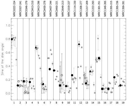
Figure 16: Disk angles for model fits with an accretion disk, for the analysis where the disk emission is fixed with respect to the narrow lines. The black points indicate the best-fit disk model for each quasar. Circular symbols indicate evidence for a disk, square symbols indicate a possible disk (inconclusive evidence, or weak to moderate evidence against a disk), while triangular symbols indicate strong evidence against the presence of a disk. White points mark fits which fall within one Jeffreys’ criterion of the best fit, and these can be seen in all cases to be consistent with the best-fit disk angle. All angles derived from non-best-fit disk cases are plotted in pale grey.

7.4 Relationships with radio source size

Figure 17 shows, for the new analysis, sine disk angle plotted against projected linear source size, which if the radio jets are perpendicular to the disks should be correlated due to geometric effects. Fixing the disk at the redshift of the NLR has strengthened this from a $1\sigma$ correlation, in the case that the model allowed a disk velocity shift (see Figure 8), to a $2\sigma$ correlation (Kendall $\tau$ coefficient 0.779, probability that a correlation exists 97%). This correlation remains at a significance level of $2\sigma$ if the CSS sources are removed from the sample (Kendall $\tau$ coefficient 0.982, probability that a correlation exists 96%).

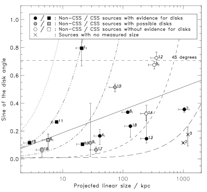
Figure 17: Sine best-fit disk angles versus the projected linear size of the quasar in kpc for the analysis in which the disk is fixed at the redshift of the NLR. The disk angle error bars include both the errors returned from the individual fits and a systematic error calculated from the variation in results from using different random seeds to initialise the Monte Carlo engines, added in quadrature, but do not take into account any error due to model selection. The non-CSS FRII sources are plotted with circles, and CSS sources are plotted with squares. The two sources plotted with crosses are core-dominated sources without measured projected sizes. The black points have weak to strong evidence for a disk, grey points have possible disks, and the white points have Bayesian evidence against the presence of a disk. Index numbers are matched to source names in Table 1. The black line shows the best linear fit to all sources excluding the core-dominated sources. There is a $2\sigma$ correlation by Kendall’s $\tau$ test between the sine of the disk angle and the projected size both for all sources excluding the core-dominated sources, and for the 11 non-CSS FRII sources. The dotted, dot-dot-dot-dashed, dot-dashed, dashed and long-dashed lines show loci of constant deprojected size, for 10 kpc, 25 kpc, 100 kpc, 1 Mpc and 5 Mpc respectively.

The source sizes were deprojected using the method in Section 6.3, and the resultant sizes are given in Table 13, with those from the original analysis for comparison. A histogram of the deprojected sizes is shown in Figure 18; the fitted angles from the new analysis deproject the source sizes to a slightly narrower range than the original analysis (see Figure 9). This does not imply a preference for the models with no disk shift, since the range of deprojected sizes merely gives an indication as to the typical size to which a source expands before it becomes quiescent.

			Proj.	Deproj.	Deproj.
			source	source	source
Quasar		Type	size	size (kpc)	size (kpc)
			(kpc)	(No disk	(Disk shift
				shift)	allowed)
1	MRC0222-224	CSS	20.6	$26\pm^{5}_{2}$	$28\pm^{8}_{1}$
2	MRC0327-241	CD	–	–	–
3	MRC0346-279	CD	–	–	–
4	MRC0413-210	FRII	41.2	$250\pm^{150}_{50}$	$550\pm^{70}_{80}$
5	MRC0413-296	FRII	330.4	$490\pm^{20}_{20}$	$520\pm^{80}_{30}$
6	MRC0430-278	CSS	5.7	$42\pm^{42}_{10}$	$380\pm^{109000}_{370}$
7	MRC0437-244	FRII	1045.9	$2950\pm^{170}_{120}$	$3430\pm^{100}_{360}$
8	MRC0450-221	FRII	120.0	$360\pm^{10}_{10}$	$530\pm^{30}_{40}$
9	MRC0549-213	FRII	28.7	$250\pm^{1400}_{180}$	$110\pm^{360}_{60}$
10	MRC1019-227	CSS	21.2	$200\pm^{20}_{20}$	$140\pm^{90}_{10}$
11	MRC1114-220	CSS	$<$ 7.9	$<30\pm^{9}_{2}$	$<14\pm^{7}_{1}$
12	MRC1208-277	FRII	359.3	$500\pm^{30}_{30}$	$1410\pm^{330}_{100}$
13	MRC1217-209	FRII	245.9	$1700\pm^{480}_{1060}$	$1700\pm^{480}_{1060}$
14	MRC1222-293	FRII	242.7	$750\pm^{140}_{30}$	$3240\pm^{660}_{1350}$
15	MRC1301-251	FRII	73.6	$140\pm^{10}_{10}$	$160\pm^{90}_{50}$
16	MRC1349-265	CSS	4.5	$69\pm^{260}_{14}$	$69\pm^{860}_{20}$
17	MRC1355-215	FRII	35.6	$550\pm^{410}_{130}$	$480\pm^{160}_{160}$
18	MRC1355-236	FRII	132.6	$570\pm^{290}_{10}$	$760\pm^{220}_{100}$
19	MRC1359-281	CSS	2.8	$24\pm^{2}_{4}$	$37\pm^{5}_{7}$

Table 13: Summary of projected and deprojected source sizes. Columns 1 and 2: Quasar index and MRC name; Column 3: Source type – CD indicates sources with core-to-lobe radio flux ratio at 10 GHz of greater than 1, CSS indicates sources with $\alpha_{\mathrm{opt}}>0.5$ and projected source sizes $<$ 25 kpc, FRII indicates non-CSS FRII, which encompasses all other sources; Column 4: Projected source sizes in kpc (sources of these values are given in Table 8); Column 5: Deprojected source sizes in kpc, calculated using the fitted disk angles from the models in which the accretion disk is fixed at the same redshift as the NLR; Column 6: Deprojected source sizes in kpc, calculated using the fitted disk angles from the models in which the accretion disk is allowed to have a different redshift from the NLR.

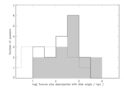
Figure 18: The solid black line shows source sizes deprojected with the fitted disk angles from the models where the disk emission is fixed at the same redshift as the NLR (see Table 13). The source sizes from deprojecting with the fitted angles from the analysis in which the disk emission is allowed to shift with respect to the NLR are shaded in grey. The projected sizes are plotted with a dotted line. Note that the two core-dominated sources have no measured size and are therefore excluded.

Figure 19 shows the cumulative distribution of the deprojected source size for the analysis of the models with the disk fixed at the redshift of the NLR. This distribution is marginally more consistent with the comparison models of uniformly expanding sources than the distribution found in the original analysis (see Figure 10). Both distributions are consistent, within the limits of small number statistics, with the picture of sources expanding uniformly up to some cut-off size, though there are indications in both cases of an excess of small sources.

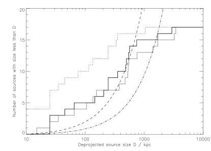
Figure 19: Cumulative distribution of source sizes deprojected using the best-fit disk angles from the models where the disk emission is fixed at the same redshift as the NLR (solid line). The projected source sizes (dotted line) and the source sizes deprojected with the angles from the analysis where the disk emission is allowed to shift with respect to the NLR (grey line) are shown for comparison. The curves show the predicted distribution if the heads of the sources are expanding at a constant rate; the dot-dashed line is normalised at the deprojected size of the largest source in the sample, the dashed line is normalised at 1 Mpc. Note that the two core-dominated sources have no measured size, and are boosted into this sample by strong core emission, and are therefore excluded from this plot.

7.5 Relationships with radio luminosity

The sine best-fit disk angles for the analysis with the accretion disks fixed at the NLR redshift are plotted against the 178 MHz radio luminosity in Figure 20. These angles are consistent with the envelope of angles predicted by the receding torus model. However, the correlation seen between the sine of the disk angle and the low-frequency radio luminosity in the original analysis, at a significance of $>1.5\sigma$ according to Kendall’s $\tau$ test, has now fallen to $<0.5\sigma$ (Kendall’s $\tau$ coefficient 0.105, probability of correlation 25%). This illustrates the strong dependence of the analysis results on the model assumptions, such that a large change in fitted angle for only two quasars is enough to disrupt this correlation.

In order the test the fragility of the luminosity – disk angle correlation, the statistical analysis was repeated 24 times, with the disk angle modified in each case by a Gaussian scatter with standard deviation of 2.16, the standard deviation of the distribution of differences between the disk angles with the disk fixed at the redshift of the NLR, and the disk angles fitted when the accretion disk was allowed a velocity shift. Only 8 out of 24 test correlations have higher significance than the original correlation between luminosity and disk angle of a disk not fixed with respect to the NLR, which has a significance of $1.8\sigma$; however, 13 out of 24 test correlations have a significance of $>1.5\sigma$. A larger sample of quasars might go some way towards confirming whether this is a real correlation, but it is clearly necessary to fully test a wider range of emission models.

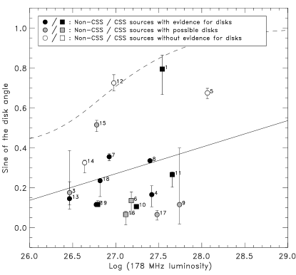
Figure 20: Sine best-fit disk angles versus logarithmic 178 MHz luminosity. The disk angle error bars include both the errors returned from the individual fits and a systematic error calculated from the variation in results from using different random seeds to initialise the Monte Carlo engines, added in quadrature, but do not take into account any error due to model selection. The non-CSS FRII sources and core-dominated sources are plotted as circles, and CSS sources are plotted as squares. The black points have weak to strong evidence for a disk, the grey points have possible disks (there is inconclusive evidence, or weak to moderate evidence against a disk) and the white points have strong evidence against a disk. Index numbers are matched to source names in Table 1. The best-fit line (minimising $\chi^{2}$) is shown in black. The dashed line shows the radio luminosity-dependent critical angle (following Willott et al. (2000)) with fiducial angle $45{}^{\circ}$ at $\log L_{178\mathrm{MHz}}$= 27, and minimum quasar fraction 10%.

7.6 Distribution of angles

The cumulative probability distribution for the disk angles and the theoretical distribution of jet angle for different values of the Lorentz factor is shown in Figure 21. With the assumption that the axis of the accretion disk is coincident with the radio jets, then the distribution of disk angles is consistent with a value of the jet Lorentz factor around $\gamma\sim 20$, as for the previous analysis (see Section 6.5).

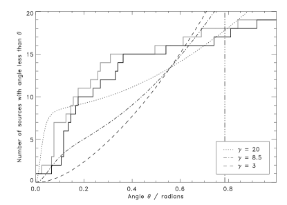
Figure 21: The cumulative distribution of the best-fit disk angles from the analysis in which the disk redshift is fixed at the redshift of the NLR (solid black line). The grey line shows the cumulative distribution for the best-fit disk angles for the analysis in which the accretion disk is allowed to shift with respect to the NLR. The curves show the theoretical distributions of jet angle, modelled from the Jackson & Wall (1999) relation and normalised up to an angle of $45{}^{\circ}$, for different values of the Lorentz factor: the dashed line shows the expected cumulative distribution for $\gamma=3$, the dot-dashed line for $\gamma=8.5$, and the dotted line for $\gamma=20$. The vertical dot-dot-dot-dashed line indicates a fitted disk angle of $45{}^{\circ}$.

7.7 Discussion

The fitted disk angles have proved to be only partially robust to a change in the model in which the accretion disk is fixed at the same redshift as the NLR, although the majority were consistent. The small number of objects in this sample make it difficult to judge whether the disappearance of the disk angle – low-frequency radio luminosity correlation in this new analysis occurs because the initial results are a fluke, or is a genuine effect from the alteration of the models. Since it is not clear that the narrow lines and accretion disk should be fixed at the same redshift, this new analysis should serve as a measure of the fragility of the results with respect to a change in the model.

8 Conclusions

All bar one of the 19 quasars are best fitted with an emission model which includes more than one component of broad-line emission, in both analyses; there is overwhelming evidence that in this sub-sample of quasars, a simple one-component broad-line emission model is insufficient to describe the physical processes at work. There is strong Bayesian evidence that ten out of nineteen quasars from the analysis in which a shift is permitted between the BLR and NLR possess accretion disks, and all but one are consistent with the emission model of a circular Keplerian accretion disk in addition to a single-peaked, symmetric emission line arising from a separate BLR. The one quasar for which this does not apply appears to have very complex broad emission, consisting of at least three components. If the model does not allow for a shift between the BLR and NLR, strong evidence for disks is seen in eight out of the nineteen sources, and all but three are consistent with the presence of a circular accretion disk.

Eracleous & Halpern (1994), Eracleous & Halpern (2003) and Strateva et al. (2003) found that only 3 – 20$\%$ of AGN have obvious double-peaked lines (see Section 1.2), in contrast to the $\sim$ 84 – 95% of this sample of quasars which were found to be consistent with the presence of a thin, optically-emitting accretion disk, despite only a few of the line profiles appearing obviously double-peaked to the eye. It may be that accretion disk emission has been seen in so few AGN because single-peaked broad emission lines, arising from fast-moving clouds located outside the thin disk or from a wind originating from the disk itself, have a tendency to swamp the disk emission. In these cases, a complex model and high signal-to-noise ratio spectra are required in order to retrieve the accretion disk contribution to the emission. It is therefore essential to extend this analysis to a larger sample of low-radio-frequency-selected quasars; optically-selected quasars are predicted to cover a narrower range in disk angles, as even lightly reddened quasars (at $\sim 45{}^{\circ}$) are much more likely to fall through the magnitude limit of a survey, and the optical emission may be angle dependent.

There is a possible correlation of the fitted disk angles with the projected source size, in agreement with the expected projection effects if the accretion disk is perpendicular to the jet. There are two CSS sources which do not appear to lie on the same relation as the other sources: MRC0222-224 seems to be an intrinsically smaller and more reddened source than the others, while MRC1114-220 may either be an outlier, or have a precessing or misaligned disk. When deprojected using the best-fit disk angles, the source sizes are consistent with a model in which the accretion disk is perpendicular to the radio jets, and the heads of the radio jets expand at approximately constant speed up to a size $\sim 1$ Mpc; the paucity of sources larger than this limit can be explained by the average duty cycle of these AGN.

The distribution of fitted disk angles is consistent with the calculation of expected jet angles for Doppler-boosted jets with Lorentz factors of $\sim$ 20, if the accretion disk rotation axis and radio jets are assumed to be coincident. The calculated jet angle distribution may match the disk angle distribution better if a more physically reasonable model was used for the jet, with a core of higher Lorentz factor than the surrounding jet sheath, as opposed to this simple single Lorentz factor model.

There is a weak correlation ($>1.5\sigma$ significance by Kendall’s $\tau$ test) between the low-frequency radio luminosity and the sine of the angle between the accretion disk axis and the line of sight. This is predicted by the receding torus model of Lawrence (1991) if the accretion disks are perpendicular to the radio jets, such that the disk angles match the jet angles. In this model, the dust is sublimated by the AGN nucleus, leading to larger opening angles of the obscuring dusty torus for more radio-luminous sources, and hence quasars are seen up to larger jet angles. The largest accretion disk angle measured is 48^∘, which is consistent with the opening angle predicted for powerful FRII radio sources. A larger sample size is needed to confirm the radio luminosity – disk angle correlation, but this is vital, as it would yield the first direct test of the receding torus model. It should be noted that when the analysis was performed again with the models in which the accretion disk was fixed at the redshift of the NLR, this result disappeared, and so the radio luminosity – disk angle correlation is strongly dependent on the model used.

A study of the velocity shifts between the line components revealed the single-peaked broad lines to be formed at similar redshifts to the narrow lines. The disk emission tended to be redshifted with respect to these lines for high-$z$ sources and blueshifted for lower-$z$ sources. Since the accretion disk is expected to be at the systemic velocity, this would imply that the single-peaked broad lines and the narrow lines are formed in outflows for more luminous, high-$z$ sources, and in infalling clouds for closer, less luminous sources. Such a scenario could arise if powerful winds were causing outflows of gas from the high-$z$, luminous sources, while these winds have stalled in the less-luminous quasars seen at $z<1$, resulting in infall of the gas back towards the galaxy nucleus.

The results of this paper are all dependent on the validity of the disk model used in the Bayesian fitting. This model, taken from Chen & Halpern (1989), describes a circular, Keplerian disk. The illuminating flux from the central black hole was modelled as falling off with a radial exponent of 3. In order to investigate the effects of range of permutations to this basic model, such as a variety of disk emissivities and warped or elliptical disks, greater spectral resolution, a larger quasar sample size, and in particular, multi-epoch data to study the variability of the emission line profiles are required.

Appendix A Tests for stability of the fitting

Detailed tests were run on two of the quasars selected at random (MRC0437-244 and MRC0450-221), in order to check the Bayesian routines for stability. In each set of tests, one of the BayeSys3 parameters was changed: the Bayesian random seed; the rate at which the Monte Carlo exploration focuses in on the region of maximum likelihood; and the ensemble of parallel explorations of the parameter space during the Monte Carlo optimisation. Plots of the posterior probabilities of the disk parameters were created, each test being overlaid in a different shade, to identify fits in which the posterior probability converged in a different region to the majority of the fits.

An example of one of the stability tests is shown in Figure 4: this shows the convergence of some of the disk parameters for MRC0450-221, as well as the correlations between these parameters, when the Bayesian fitting is initialised with five different random seeds. The posterior probability distribution for each seed is plotted in a different shade of grey. The local velocity dispersion, $\Delta v$, of the disk material converges in two slightly different regions of parameter space, depending on the Bayesian seed, though these areas are within a reasonable error bound of each other. The local minima do not have vastly different evidence values in this case ($\Delta\ln(\mathrm{Evidence})\sim 2.5$ between the highest and lowest evidence cases); this is due to the fact that the profile of the disk emission varies only weakly with the local velocity dispersion (Strateva et al., 2003). The variation in velocity dispersion was similar through all of the parameters tested: all other parameters were shown to be stable in each of the tests for MRC0450-221. All parameters were stable in the tests for MRC0437-244.

In addition, similar tests were made in which the Bayesian fitting parameters were unchanged, but the spectra were altered. The first of these tests added Gaussian random noise to the spectrum, with FWHM of 5% of the data values, in order to see qualitatively what effect greater noise has on the fitting process. For MRC0450-221, the posterior probability for the local velocity dispersion occupied a similar region in parameter space to the total space occupied by all fits in the test with different Bayesian random seeds; it appears that the velocity dispersion parameter is constrained to a fairly large region of parameter space, and within this, for some tests, local minima are found. For MRC0437-241, the parameters constrain in similar regions independent of the noise added.

The second of these tests was the fitting of spectra smoothed with boxcar widths of 3, 5, 7 and 9 pixels, where each pixel has a scale of approximately 2 Å. For MRC0437-244, the smoothed spectrum allowed the probability to constrain marginally more tightly, but in the same regions. This was also true of MRC0450-221 for the boxcar smoothing widths of 3, 5 and 7 pixels. At a boxcar width of 9 pixels, the posterior probability distributions of the fit alter significantly, as real structure has been lost from the spectrum.

References

- Amico et al. (2002) Amico, P., Cuby, J.-G., Devillard, N., Jung, Y., Lidman, C., 2002, Isaac Data Reduction Guide
- Antonucci (1993) Antonucci, R., 1993, ARA&A, 31, 473
- Antonucci & Miller (1985) Antonucci, R. R. J., Miller, J. S., 1985, ApJ, 297, 621
- Bachev (1999) Bachev, R., 1999, A&A, 348, 71
- Bahcall & Soneira (1980) Bahcall, J. N., Soneira, R. M., 1980, ApJS, 44, 73
- Baker et al. (1999) Baker, J. C., Hunstead, R. W., Kapahi, V. K., Subrahmanya, C. R., 1999, ApJS, 122, 29
- Baker et al. (2002) Baker, J. C., Hunstead, R. W., Athreya, R. M., Barthel, P. D., de Silva, E., Lehnert, M. D., 2002, ApJ, 568, 592
- Baldwin (1977) Baldwin, J. A., 1977, ApJ, 214, 679
- Barthel (1989) Barthel, P. D., 1989, ApJ, 336, 606
- Bird et al. (2008) Bird, J., Martini, P., Kaiser, C., 2008, ApJ, 676, 147
- Brown et al. (1989) Brown, L. M. J., Robson, E. I., Gear, W. K., Hughes, D. H., Griffin, M. J., Geldzahler, B. J., Schwartz, P. R., Smith, M. G., Smith, A. G., Shepherd, D. W., Webb, J. R., Valtaoja, E., Terasranta, H., Salonen, E., 1989, ApJ, 340, 129
- Capriotti et al. (1979) Capriotta, E., Foltz, C., Byard, P., 1979, ApJ, 230, 681
- Chen et al. (1989) Chen, K., Halpern, J. P., Filippenko, A. V., 1989, ApJ, 339, 742
- Chen & Halpern (1989) Chen, K., Halpern, J. P., 1989, ApJ, 344, 115