Homogeneous hypersurfaces in $\mathbb{C}^{3}$, associated with a model CR-cubic

Abstract.

The model 4-dimensional CR-cubic in $\mathbb{C}^{3}$ has the following "model" property: it is (essentially) the unique locally homogeneous 4-dimensional CR-manifold in $\mathbb{C}^{3}$ with finite-dimensional infinitesimal automorphism algebra $\mathfrak{g}$ and non-trivial isotropy subalgebra. We study and classify, up to local biholomorphic equivalence, all $\mathfrak{g}$-homogeneous hypersurfaces in $\mathbb{C}^{3}$ and also classify the corresponding local transitive actions of the model algebra $\mathfrak{g}$ on hypersurfaces in $\mathbb{C}^{3}$.

1. introduction

The most interesting objects in CR-geometry are CR-manifolds with symmetries, i.e. CR-manifolds, admitting (local) actions of Lie groups by holomorphic transformations. If such an action is (locally) transitive, then the manifold is called (locally) holomorphically homogeneous (or just homogeneous). Locally homogeneous manifolds are "the same in all points", i.e. the germs of a locally homogeneous manifold at any two points are biholomorphically equivalent. Among all homogeneous CR-manifolds one can single out so-called model manifolds - algebraic CR-submanifolds in $\mathbb{C}^{N}$ with maximal-dimensional automorphism groups. As it was demonstrated in [9],[17],[5], the properties of model manifolds determine in many aspects the properties of general CR-manifolds. In this paper some interplay between a model 4-manifold in $\mathbb{C}^{3}$ and homogeneous hypersurfaces in $\mathbb{C}^{3}$ is studied.

To work with homogeneous CR-manifolds and their symmetry groups and algebras we give a few definitions.

Consider in the complex space $\mathbb{C}^{N}$ a germ $M_{p}$ of a generic real-analytic CR-submanifold $M$ at a point $p\in M$ (we suppose that all CR-submanifolds are real-analytic and generic if not otherwise mentioned). We consider the following objects:

1) $\it\mathfrak{aut}M_{p}$ - the Lie algebra of germs at the point $p$ of vector fields of the form

$$2\mbox{Re}\,\left(f_{1}(z)\frac{\partial}{\partial z_{1}}+\dots+f_{N}(z)\frac{\partial}{\partial z_{N}}\right),$$

which are tangent to $M$ at each point, and the functions $f_{j}(z)$ are holomorphic in a neighborhood of $p$. We call such vector fields holomorphic vector fields on $M$ in a neighborhood of $p$. Clearly these vector fields are exactly that ones which generate local actions of Lie groups on $M$ by transformations, holomorphic in a neighborhood of $p$ in $\mathbb{C}^{N}$. The Lie algebra $\it\mathfrak{aut}M_{p}$ is called the infinitesimal automorphism algebra of $M$ at $p$. If $\it\mathfrak{aut}M_{p}$ is finite-dimensional, then all vector fields from this algebra can be defined in the same neighborhood and there exists a connected simply-connected Lie group, acting on $M$ locally by holomorphic transformations in a neighborhood of the point $p$, such that its tangent algebra is isomorphic to $\it\mathfrak{aut}M_{p}$ and the vector fields from $\it\mathfrak{aut}M_{p}$ are the infinitesimal generators of the action. We denote this local group by $\it AutM_{p}$ and call it the local holomorphic automorphism group of $M$ at $p$.

2) $\it\mathfrak{aut}_{p}M_{p}$ - the Lie subalgebra in $\it\mathfrak{aut}M_{p}$, which consists of germs of vector fields from $\it\mathfrak{aut}M_{p}$, vanishing at $p$. This algebra is called the stability subalgebra of $M$ at the point $p$ or the isotropy subalgebra. If $\it\mathfrak{aut}M_{p}$ is finite-dimensional, then $\it\mathfrak{aut}_{p}M_{p}$ is naturally identified with the tangent algebra of the stability group $\it Aut_{p}M_{p}$, which consists of holomorphic automorphisms of the germ, fixing the point $p$.

A local action of a finite-dimensional real Lie algebra $\mathfrak{h}$ on the germ $\mathbb{C}^{N}_{p}$ of the complex space $\mathbb{C}^{N}$ at a point $p$ is a homomorphism $\varphi:\,\mathfrak{h}\longrightarrow\mathfrak{aut}\,\mathbb{C}^{N}_{p}$. If $M$ is a CR-submanifold in $\mathbb{C}^{N}$, passing through $p$, we say that $\mathfrak{h}$ acts transitively on $M_{p}$ (or that $\mathfrak{h}$ acts locally transitively on $M$ at the point $p$), if the linear space, spanned by the values at the point $p$ of the vector fields from $\varphi(\mathfrak{h})$, which are tangent to $M$, coincides with $T_{p}M$. The germ $M_{p}$ is called homogeneous in this case, and the manifold $M$ is called locally homogeneous at $p$. If $M$ is locally homogeneous at all points, then we call it just locally homogeneous. For more information about possible equivalent definitions of homogeneous CR-manifolds we refer to [18].

With any local action of a Lie algebra $\mathfrak{h}$ we can associate a local action of a local Lie group $H$ with tangent algebra $\mathfrak{h}$ and consider the orbits of this action. These orbits are locally homogeneous CR-manifolds and their local homogeneity is provided by the Lie algebra $\mathfrak{h}$. We call this collection of orbits locally homogeneous manifolds, associated with the Lie algebra $\mathfrak{h}$.

Coming back to homogeneous CR-manifolds in $\mathbb{C}^{3}$, we firstly mention E.Cartan’s classification theorem for homogeneous hypersurfaces in $\mathbb{C}^{2}$ (see [8]). Due to this theorem, the following trichotomy holds for a locally homogeneous hypersurface in $\mathbb{C}^{2}_{z,w}$:

(1) $\mbox{dim}\,\mathfrak{aut}M_{p}=\infty,$ which occurs if and only if $M$ is locally biholomorphically equivalent to the hyperplane $\mbox{Im}\,w=0$ (the Levi-flat case).

(2) $\mbox{dim}\,\mathfrak{aut}M_{p}=8,$ which occurs if and only if $M$ is locally biholomorphically equivalent to the unit sphere $|z|^{2}+|w|^{2}=1$.

(3) $\mbox{dim}\,\mathfrak{aut}M_{p}=3,$ which occurs if and only if $M$ is locally biholomorphically equivalent to one of Cartan’s homogeneous surfaces (see [8] for details).

Note that due to a classical result of H.Poincare [16], all other hypersurfaces in $\mathbb{C}^{2}$ have infinitesimal automorphism algebras of dimensions $\leq 2$.

Hence we have the following rigidity phenomenon for germs of Levi non-degenerate homogeneous hypersurfaces in $\mathbb{C}^{2}$: any such germ is either a germ of the model surface (i.e. the sphere in our case) and has maximal-dimensional infinitesimal automorphism algebra, or it is holomorphically rigid, i.e its stability subalgebra is trivial.

The classification of homogeneous hypersurfaces in $\mathbb{C}^{3}$ is not complete yet. In the case of Levi non-degenerate hypersurfaces with high-dimensional isotropy subalgebras the classification was obtained by A.Loboda (see [14],[15]). In the Levi degenerate case the full classification was obtained by G.Fels and W.Kaup. To describe their results we give the following definition: a CR-submanifold $M$ in $\mathbb{C}^{N}$ is called holomorphically degenerate, if in a neighborhood of any point $p\in M$ there exists a non-zero holomorphic vector field on $M$, which belongs to the complex tangent space of $M$ at each point. In this case it is not difficult to see that $\mbox{dim}\,\mathfrak{aut}\rm M_{p}=\infty.$ Otherwise $M$ is called holomorphically non-degenerate. In particular, all Levi non-degenerate hypersurfaces are holomorphically non-degenerate. In case of Levi degenerate hypersurface in $\mathbb{C}^{3}$ this non-degeneracy condition is equivalent to the 2-nondegeneracy, in a general point, which is some condition on the defining function of the hypersurface (see [2] for details). For a 2-nondegenerate hypersurface the Levi form has rank 1 at each point and $\mbox{dim}\,\it\mathfrak{aut}M_{p}<\infty.$

Now we can formulate G.Fels and W.Kaup’s classification theorem. Due to this theorem, the following trichotomy holds for a locally homogeneous Levi degenerate hypersurface in $\mathbb{C}^{3}$:

(1) $\mbox{dim}\,\mathfrak{aut}M_{p}=\infty,$ which occurs if and only if $M$ is locally biholomorphically equivalent to a direct product $M^{3}\times\mathbb{C}$, where $M^{3}\subset\mathbb{C}^{2}$ is one of the homogeneous hypersurfaces in $\mathbb{C}^{2}$ from E.Cartan’s list specified above (holomorphically degenerate case).

(2) $\mbox{dim}\,\mathfrak{aut}M_{p}=10,$ which occurs if and only if $M$ is locally biholomorphically equivalent to the tube over the future light cone: $y_{3}^{2}=y_{1}^{2}+y_{2}^{2},y_{3}>0,\,y_{j}=\mbox{Im}\,z_{j},\,(z_{1},z_{2},z_{3})\in\mathbb{C}^{3}$.

(3) $\mbox{dim}\,\mathfrak{aut}M_{p}=5,$ which occurs if and only if $M$ is locally biholomorphically equivalent to the tube over an affinely homogeneous hypersurface in $\mathbb{R}^{3}$ from some list, specified in [12].

Hence, in the same way as in E.Cartan’s case, we have the rigidity phenomenon for germs of holomorphically non-degenerate locally homogeneous hypersurfaces in $\mathbb{C}^{3}$: any such germ is either a germ of the model surface (i.e. the tube over the future light cone in that case) and has maximal-dimensional infinitesimal automorphism algebra, or it is holomorphically rigid, i.e its stability subalgebra is trivial.

We study the class of locally homogeneous hypersurfaces in $\mathbb{C}^{3}$ with the following property: the local homogeneity of these surfaces is provided by one of the model algebras in $\mathbb{C}^{3}$ - the unique 5-dimensional model algebra for the class of 4-dimensional holomorphically non-degenerate (or, equivalently, totally non-degenerate [7]) CR-manifolds in $\mathbb{C}^{3}$. This algebra is the infinitesimal automorphism algebra $\mathfrak{g}$ of the model 4-dimensional CR-cubic $C$, given by the following equations:

$$\mbox{Im}\,w_{2}=|z|^{2},\,\mbox{Im}\,w_{3}=2\mbox{Re}\,(z^{2}\bar{z}),\,(z,w_{2},w_{3})\in\mathbb{C}^{3}$$

(this notation is related to a natural gradation of the coordinates in $\mathbb{C}^{3}$, see section 2).

Due to V.K.Beloshapka, V.V.Ezhov and G.Schmalz (see [7]), the model properties of the cubic $C$ are given by the following trichotomy for a 4-dimensional locally homogeneous CR-manifold $M$ in $\mathbb{C}^{3}$:

(1) $\mbox{dim}\,\mathfrak{aut}M_{p}=\infty$, which occurs if and only if $M$ is locally biholomorphically equivalent to a direct product $M^{3}\times\mathbb{R}^{1},\,M^{3}\subset\mathbb{C}^{2}_{z_{1},z_{2}},\,\mathbb{R}^{1}\subset\mathbb{C}^{1}_{z_{3}}$ (the holomorphically degenerate case).

(2) $\mbox{dim}\,\mathfrak{aut}M_{p}=5$, which occurs if and only if $M$ is locally biholomorphically equivalent to the cubic $C$.

(3) $\mbox{dim}\,\mathfrak{aut}M_{p}=4,\,\mbox{dim}\,\mathfrak{aut}_{p}M_{p}=0$ for all other manifolds (the rigidity phenomenon).

It is proved also in [7] that the cubic $C$ is the most symmetric holomorphically non-degenerate 4-manifold in $\mathbb{C}^{3}$: $\mbox{dim}\,\mathfrak{aut}M_{0}\leq\mbox{dim}\,\mathfrak{aut}C_{0}$, and the equality holds only for manifolds, locally biholomorphically equivalent to the cubic. The automorphism group $G$ and the infinitesimal automorphism algebra $\mathfrak{g}$ of the cubic are described in the next section.

We associate with the cubic $C$ some (locally) homogeneous hypersurfaces in $\mathbb{C}^{3}$ in two different ways.

The first one is to consider the natural action of the 5-dimensional polynomial transformation group $G$ (or, equivalently, of the model algebra $\mathfrak{g}$) in the ambient space $\mathbb{C}^{3}$. Since the group is of dimension 5, we conclude that the cubic is a singular 4-dimensional orbit of this action, but general orbits are of dimension 5. This approach was realized in [6]. Note that according to the above trichotomy for a homogeneous 4-manifold in $\mathbb{C}^{3}$ this machinery for the construction of homogeneous hypersurfaces in $\mathbb{C}^{3}$, associated with a homogeneous 4-manifold, is the only possible, i.e. the obtained in [6] class of hypersurfaces is (essentially) the class of all locally homogeneous hypersurfaces, associated in the natural sense with locally homogeneous 4-manifolds in $\mathbb{C}^{3}$ (in the category of non-degenerate manifolds). In section 2 we give a review of the results of [6] and also give another (tube) realization to the obtained in [6] foliation to orbits (case $A$ in the theorem below). It helps us to recognize one special orbit as one of the hypersurfaces from [12] and also helps us to find an interesting realization of the cubic $C$ as the tube over the twisted cubic in $\mathbb{R}^{3}$. In section 3 we classify the obtained homogeneous hypersurfaces and compute their automorphism groups. In particular, we prove an analogue of the Poincare-Alexander theorem (see [16],[1]) for the orbits under consideration.

The second one is to consider all homogeneous hypersurfaces in $\mathbb{C}^{3}$, associated with the abstract model Lie algebra $\mathfrak{g}$. The approach in this case is analogue to E.Cartan’s approach in the classification problem for hypersurfaces in $\mathbb{C}^{2}$. We find all possible realizations of the abstract Lie algebra $\mathfrak{g}$ as an algebra of holomorphic vector fields in $\mathbb{C}^{3}$, acting transitively on hypersurfaces, and thus find all possible orbits of the corresponding actions - they form the desired class of homogeneous hypersurfaces in $\mathbb{C}^{3}$ (we call these hypersurfaces $\mathfrak{g}$-homogeneous). This approach is realized in section 4. In section 5 we classify the obtained homogeneous hypersurfaces up to local biholomorphic equivalence and compute their infinitesimal automorphism algebras (and hence the corresponding local automorphism groups). As a result we prove the following classification theorem for $\mathfrak{g}$-homogeneous hypersurfaces in $\mathbb{C}^{3}$:

Main theorem. (1) The model algebra $\mathfrak{g}$ has 4 types of local transitive actions on hypersurfaces in $\mathbb{C}^{3}$ - actions of type $A,A_{1},A_{0}$ and $B$, described in section 5. Any two actions of different types are inequivalent. The corresponding orbits look as follows.

$$\mbox{TYPE}\,\,A:\,N_{\nu}^{\pm}=\left\{(y_{3}-3y_{1}y_{2}+2y_{1}^{3})^{2}=\pm\nu(y_{2}-y_{1}^{2})^{3},\,\pm(y_{2}-y_{1}^{2})>0\right\},\,\nu\geq 0,$$

$$N^{0}=\left\{y_{2}=y_{1}^{2},\,y_{3}\neq y_{1}^{3}\right\}.$$

$$\mbox{TYPE}\,\,A_{1}:\,\,\,S_{\gamma}=\left\{y_{3}=\gamma y_{1}^{3}+\frac{y_{2}^{2}}{y_{1}},y_{1}\neq 0\right\},\,\gamma\in\mathbb{R}.$$

$$\mbox{TYPE}\,\,A_{0}:\,\,\,Q_{\beta}=\{y_{3}=\beta y_{1}^{3}+2y_{2}x_{1},\,y_{1}\neq 0\},\,\beta\in\mathbb{R}.$$

$$\mbox{TYPE}\,\,B:\,\,\,\Pi_{\delta}=\{y_{2}=\delta y_{1},\,y_{1}y_{2}\neq 0\},\,\delta\in\mathbb{R}^{*}.$$

Here $z_{k}=x_{k}+iy_{k}$.

(2) Any $\mathfrak{g}$-homogeneous hypersurface in $\mathbb{C}^{3}$ is locally biholomorphically equivalent to one of the following pairwise non-equivalent homogeneous hypersurfaces in $\mathbb{C}^{3}$:

(a) Tube manifolds $N^{\pm}_{\nu}$ for $\nu>0$.

(b) Tube manifolds $S_{\pm 1}$ (the case of $S_{\gamma},\gamma\in\mathbb{R}^{*})$.

(c) The tube over the future light cone $y_{3}^{2}=y_{1}^{2}+y_{2}^{2},\,y_{3}>0$ (the case of $S_{0}$).

(d) The indefinite quadric $y_{3}=|z_{1}|^{2}-|z_{2}|^{2}$ (the case of $N^{\pm}_{0}$ and $Q_{\beta},\beta\in\mathbb{R}$).

(e) The cylinder over the unit sphere in $\mathbb{C}^{2}$: $|z_{1}|^{2}+|z_{2}|^{2}=1$ (the case of $M^{0}$).

(f) The real hyperplane $y_{3}=0$ (the case of $\Pi_{\delta},\delta\in\mathbb{R}^{*}$).

In cases (e) and (f) the infinitesimal automorphism algebras of the surfaces are infinite-dimensional; in cases (c) and (d) these algebras are well-known simple Lie algebras (see [13],[5],[9] for the description of the algebras and the corresponding local automorphism groups); in case (a) the infinitesimal automorphism algebras coincide with the model algebra $\mathfrak{g}$, and all local automorphism of the surfaces are global and belong to the group $G$; in case (b) the infinitesimal automorphism algebras are isomorphic to the model algebra $\mathfrak{g}$ (more precisely, they coincide with the algebra $A_{1}$), the corresponding local automorphism group is described in section 5, hence in cases (a) and (b) the hypersurfaces are holomorphically rigid.

Remark 1.1.  We note some interesting facts, which follow from the above classification theorem.

(1) All $\mathfrak{g}$-homogeneous hypersurfaces are locally biholomorphically equivalent to globally homogeneous hypersurfaces.

(2) All $\mathfrak{g}$-homogeneous hypersurfaces turn out to be tube manifolds over affinely homogeneous hypersurfaces in $\mathbb{R}^{3}$ in an appropriate local coordinate system (for the indefinite quadric we get the tube realization by means of a quadratic variable change, as well as for the unit sphere in the Poincare realization). Affinely homogeneous hypersurfaces in $\mathbb{R}^{3}$ were classified in [11] and [10], but the corresponding tube manifolds in $\mathbb{C}^{3}$ were not studied from the point of view of holomorphic classification and automorphism groups. Hence the present work can be considered as a step in this direction.

(3) The hypersurfaces $N^{+}_{\mu}$ for $\mu>0$, $N^{-}_{\nu}$ for $\nu>0,\nu\neq 4$ and $S_{\pm 1}$ are Levi non-degenerate and holomorphically rigid. Hence they give examples of pairwise non-equivalent locally homogeneous hypersurfaces in $\mathbb{C}^{3}$, which are not covered by the classification theorems obtained in [14],[15],[12] (the exceptional orbit $N^{-}_{4}$ is 2-nondegenerate and hence occurs in [12]).

(4) In the same way as it results in both E.Cartan’s and G.Fels-W.Kaup’s classification theorems, the following rigidity phenomenon holds: each holomorphically non-degenerate homogeneous hypersurface, generated in the specified sense by the model algebra $\mathfrak{g}$, is either extremely-symmetric (a quadric - the most symmetric Levi non-degenerate hypersurface, or the tube over the future light cone - the most symmetric 2-nondegenerate hypersurface), or it is holomorphically rigid, i.e. its isotropy subalgebra is trivial. Each of the obtained infinitesimal automorphism algebras turns out to be isomorphic to one of the model algebras in $\mathbb{C}^{3}$ (i.e. to the infinitesimal automorphism algebra of a quadric, of the cubic or of the tube over the future light cone). Thus the construction of homogeneous hypersurfaces, used in [6] and in the present paper, gives an interesting connection among model algebras in $\mathbb{C}^{3}$. It is also amazing that the obtained holomorphically degenerate hypersurfaces are in a certain sense also extremely-symmetric: the first one (the hyperplane) is the cylinder over the most symmetric hypersurface in $\mathbb{C}^{2}$ - the hyperplane $\mbox{Im}\,w=0$, and the second one is the cylinder over the most symmetric Levi non-degenerate hypersurface in $\mathbb{C}^{2}$ - the unit sphere $|z_{1}|^{2}+|z_{2}|^{2}=1$.

Remark 1.2.  Note that the above classification theorem gives a description of all possible hypersurface-type left-invariant CR-structures on the group $G=Aut(C)$ (see section 2).

The authors would like to thank W.Kaup for useful remarks, which helped to improve the text of this paper.

2. Action of the automorphism group of the cubic in the ambient space

In this section we describe the automorphism group $G$ and the infinitesimal automorphism algebra $\mathfrak{g}$ of the cubic $C$, and then give a review of the paper [6], where the action of the group $G$ in the ambient space $\mathbb{C}^{3}$ was studied and the corresponding orbits were presented explicitly. Also we present another (tube) realization of the obtained foliation of $\mathbb{C}^{3}$, given by the group $G$, which helps us to recognize one special orbit as a well-known hypersurface in $\mathbb{C}^{3}$ and find a tube realization for the model cubic $C$.

As it was mentioned in the introduction, the cubic $C$ is a homogeneous 4-dimensional CR-manifold in $\mathbb{C}^{3}$, given by the following equations:

$$\mbox{Im}\,w_{2}=|z|^{2},\,\mbox{Im}\,w_{3}=2\mbox{Re}\,(z^{2}\overline{z}),\,(z,w_{2},w_{3})\in\mathbb{C}^{3}.$$

This notation is associated with the following natural gradation of the coordinates in $\mathbb{C}^{3}$:

(1) $$[z]=1,[w_{2}]=2,[w_{3}]=3.$$

The polynomials $\mbox{Im}\,w_{2}-|z|^{2}$ and $\mbox{Im}\,w_{3}-2\mbox{Re}\,(z^{2}\overline{z})$ are homogeneous under this gradation and hence the cubic admits an action of the following group of dilations:

(2) $$z\longrightarrow\lambda z,\,w_{2}\longrightarrow\lambda^{2}w_{2},\,w_{3}\longrightarrow\lambda^{3}w_{3},\,\lambda\in\mathbb{R}^{*}.$$

This group is the isotropy subgroup $G_{0}$ of the origin in the 5-dimensional group $G=Aut(C)$. $G$ is a semidirect product of $G_{0}$ and the following polynomial group $G_{-}$, providing the homogeneity of the cubic:

$$z\mapsto z+p,$$

(3) $$w_{2}\mapsto w_{2}+2i\bar{p}z+i|p|^{2}+q_{2},$$

$$w_{3}\mapsto w_{3}+4(\mathop{\rm Re}\nolimits p)w_{2}+2i(2|p|^{2}+\bar{p}^{2})z+2i\bar{p}z^{2}+2i\mathop{\rm Re}\nolimits(p^{2}\bar{p})+q_{3},$$

$$\mbox{where}\,\,\,p\in\mathbb{C},\,q_{j}\in\mathbb{R}.$$

The infinitesimal automorphism algebra $\mathfrak{g}$ of the cubic, which can be naturally identified with the tangent algebra of $G$, is a graded Lie algebra of kind

$$\mathfrak{g}=\mathfrak{g}_{-3}+\mathfrak{g}_{-2}+\mathfrak{g}_{-1}+\mathfrak{g}_{0},$$

where the gradation for monomials is taken from (1), and the basic differential operators are graded in the following way:

$$\left[\frac{\partial}{\partial z}\right]=-1,\left[\frac{\partial}{\partial w_{2}}\right]=-2,\left[\frac{\partial}{\partial w_{3}}\right]=-3.$$

The basic vector fields from $\mathfrak{g}$ look as follows (we skip the operator $2\mbox{Re}\,(\cdot)$):

$$X_{3}=\frac{\partial}{\partial w_{3}},\,X_{2}=\frac{\partial}{\partial w_{2}},$$

$$X^{\prime}_{1}=i\frac{\partial}{\partial z}+2z\frac{\partial}{\partial w_{2}}+2z^{2}\frac{\partial}{\partial w_{3}},$$

$$X_{1}=\frac{\partial}{\partial z}+2iz\frac{\partial}{\partial w_{2}}+(4w_{2}+2iz^{2})\frac{\partial}{\partial w_{3}},$$

$$X_{0}=z\frac{\partial}{\partial z}+2w_{2}\frac{\partial}{\partial w_{2}}+3w_{3}\frac{\partial}{\partial w_{3}}.$$

Here $\mathfrak{g}_{-3}$ is spanned by $X_{3},\,\,\mathfrak{g}_{-2}=<X_{2}>,\,\mathfrak{g}_{-1}=<X_{1},X^{\prime}_{1}>,\,\mathfrak{g}_{0}=<X_{0}>$. Since $\mathfrak{g}_{0}$ is abelian, the algebra $\mathfrak{g}$ is solvable. Also note that

$$<X_{3},X_{2},X^{\prime}_{1}>$$

is an abelian ideal in $\mathfrak{g}$.

The subalgebra $\mathfrak{g}_{0}$ is the isotropy subalgebra of the origin and hence corresponds to the subgroup $G_{0}$, the nilpotent ideal $\mathfrak{g}_{-}=\mathfrak{g}_{-3}+\mathfrak{g}_{-2}+\mathfrak{g}_{-1}$ corresponds to the subgroup $G_{-}$ (this ideal coincides with the unique irreducible 4-dimensional nilpotent real Lie algebra).

The natural action of $G$ in the ambient space is given as a composition of actions (2) and (3). Note, that the polynomial $P=\mathop{\rm Im}\nolimits w_{2}-|z|^{2}$ is a relative invariant of this natural action of weight 2 (more precisely, each transformation from $G$ multiplies it by $\lambda^{2}$). Hence we have 3 kinds of orbits: those lying in the domain $\mathop{\rm Im}\nolimits w_{2}-|z|^{2}>0$ (case 1 - orbits "over the ball"), those lying in the domain $\mathop{\rm Im}\nolimits w_{2}-|z|^{2}<0$ (case 2 - orbits "over the complement to the ball"), and those lying over the quadric $\mathop{\rm Im}\nolimits w_{2}-|z|^{2}=0$ (case 3 - orbits "over a sphere").

CASE 1. In this case, as was shown in [6], for a point $(a,b,c),\mbox{Im}\,b>|a|^{2}$ we get the following orbits:

$$\mathop{\rm Im}\nolimits w_{3}=-2\mathop{\rm Re}\nolimits z^{2}\bar{z}+4\mathop{\rm Re}\nolimits z\mathop{\rm Im}\nolimits w_{2}+|\mu|(\mathop{\rm Im}\nolimits w_{2}-|z|^{2})^{\frac{3}{2}},\,\mbox{Im}\,w_{2}>|z|^{2},\mu\in\mathbb{R}.$$

Any orbit is an open smooth part of the real-analytic set

$$(\mathop{\rm Im}\nolimits w_{3}-4\mathop{\rm Re}\nolimits z\mathop{\rm Im}\nolimits w_{2}+2|z|^{2}\mathop{\rm Re}\nolimits z)^{2}=\mu^{2}(\mathop{\rm Im}\nolimits w_{2}-|z|^{2})^{3},$$

lying over $P>0$.

Any such orbit except the one with $\mu=0$ has two connected components, corresponding to two $\mu$ with opposite signs. They can be mapped to each other by the linear automorphism of the cubic

(4) $$z\rightarrow-z,w_{2}\rightarrow w_{2},w_{3}\rightarrow-w_{3}.$$

Orbits, corresponding to different $\mu^{2}$, are clearly different. Hence the family of orbits is parametrized by the non-negative parameter $\mu^{2}$.

The Levi forms of the orbits are as follows:

$$-\frac{3}{2}\mu|z|^{2}+iz\bar{w_{2}}-iw_{2}\bar{z}+\frac{3}{16}\mu|w_{2}|^{2}.$$

Then for each $\mu$ the orbits are homogeneous hypersurfaces with non-degenerate indefinite Levi form.

CASE 2. In this case, as was shown in [6], for a point $(a,b,c),\mbox{Im}\,b<|a|^{2}$ we get the following orbits:

$$\mathop{\rm Im}\nolimits w_{3}=-2\mathop{\rm Re}\nolimits z^{2}\bar{z}+4\mathop{\rm Re}\nolimits z\mathop{\rm Im}\nolimits w_{2}+|\nu|(|z|^{2}-\mathop{\rm Im}\nolimits w_{2})^{\frac{3}{2}},\,\mbox{Im}\,w_{2}>|z|^{2},\nu\in\mathbb{R}.$$

Any such orbit is an open smooth part of a real-analytic set

$$(\mathop{\rm Im}\nolimits w_{3}-4\mathop{\rm Re}\nolimits z\mathop{\rm Im}\nolimits w_{2}+2|z|^{2}\mathop{\rm Re}\nolimits z)^{2}=\nu^{2}(|z|^{2}-\mathop{\rm Im}\nolimits w_{2})^{3},$$

lying over $P<0$.

Any orbit except the one with $\nu=0$ has two connected components, corresponding to two $\nu$ with opposite signs. They can be mapped to each other by the linear automorphism (4) of the cubic. Orbits, corresponding to different $\nu^{2}$, are clearly different. Hence the family of orbits is parametrized by the non-negative parameter $\nu^{2}$.

The Levi form in this case equals

$$\frac{3}{2}\nu|z|^{2}+iz\bar{w_{2}}-iw_{2}\bar{z}+\frac{3}{16}\nu|w_{2}|^{2}.$$

The determinant of the Levi form is $(\frac{9}{32}\nu^{2}-1)$. Hence for $\nu^{2}>\frac{32}{9}$ the hypersurfaces are strictly pseudoconvex; for $\nu^{2}=\frac{32}{9}$ the orbit is Levi-degenerate, the Levi form has one non-zero eigenvalue; for $\nu^{2}<\frac{32}{9}$ the orbits have indefinite Levi form.

CASE 3. In that case straightforward calculations show that the values of the vector fields, which form the basis of the algebra $\mathfrak{g}$, have rank 4 at each point on the cubic and rank 5 at each point outside the cubic. Hence the cubic is the only singular orbit of dimension 4. As it was shown in [6], there are two orbits in that case:

$$\mbox{Im}\,w_{2}=|z|^{2},\quad\mbox{Im}\,w_{3}=2\mbox{Re}\,(z^{2}\bar{z})$$

- the cubic, and

$$\mbox{Im}\,w_{2}=|z|^{2},\quad\mbox{Im}\,w_{3}\neq 2\mbox{Re}\,(z^{2}\bar{z})$$

- the complement to the cubic on the cylindric surface $\mbox{Im}\,w_{2}=|z|^{2}$. The second orbit has two connected components, which can be mapped to each other by the linear automorphism (4) of the cubic.

To characterize globally the foliation of the space $\mathbb{C}^{3}$, given by the group $G$, note that the polynomial

$$Q=\mathop{\rm Im}\nolimits w_{3}-4\mathop{\rm Re}\nolimits z\mathop{\rm Im}\nolimits w_{2}+2|z|^{2}\mathop{\rm Re}\nolimits z$$

is also a relative invariant of the action (2)-(3) of weight 3. In terms of the relative invariant polynomials, the orbits "over the ball" are given by the condition

$$Q^{2}=\mu^{2}P^{3},\;P>0,$$

the orbits "over the complement to the ball" are given by the condition

$$Q^{2}=\nu^{2}(-P)^{3},\;P<0,$$

the orbits "over the sphere" are given by the condition

$$P=Q=0$$

- the cubic, and

$$Q\neq 0,\;P=0$$

- the complement to the cubic. The obtained description of the foliation is illustrated by the figure.

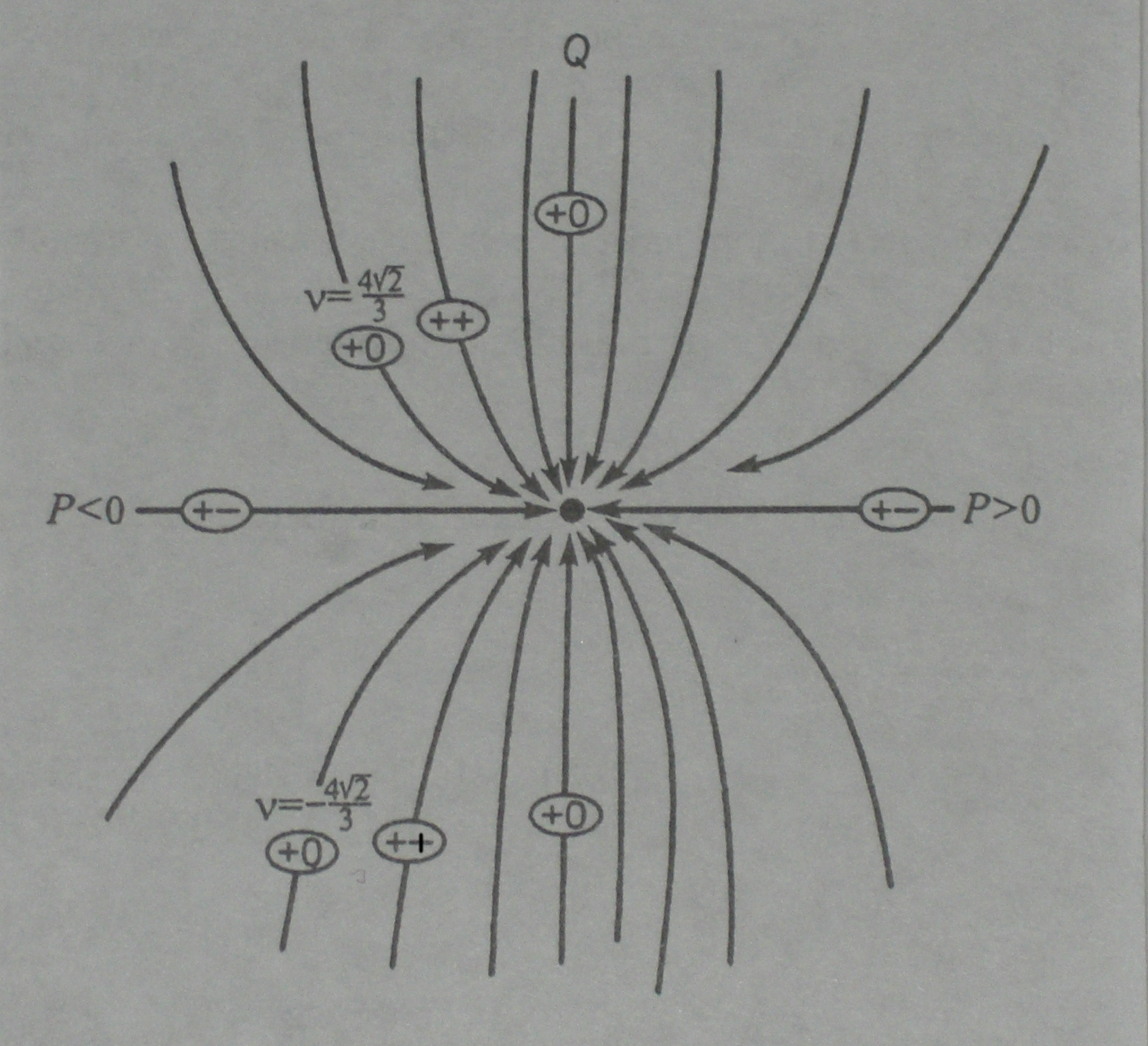
Figure 1.

Also note the following fact: the cubic $C$ is the boundary of any orbit, and, roughly saying, any two orbits $M,M^{\prime}$ "meet at $C$", but the union $M\cup M^{\prime}\cup Q$ does not form a smooth hypersurface (moreover, this union does not also decompose to smooth hypersurfaces), except the case $\mu=\nu=0$, when this union forms the smooth hypersurface

(5) $$Q=\mathop{\rm Im}\nolimits w_{3}-4\mathop{\rm Re}\nolimits z\mathop{\rm Im}\nolimits w_{2}+2|z|^{2}\mathop{\rm Re}\nolimits z=0.$$

Now we give a tube realization for the obtained foliation in $\mathbb{C}^{3}$, generated by the group $G$. To do so, remember, that one of the obtained orbits - corresponding to $\nu=\frac{4\sqrt{2}}{3}$ - is Levi degenerate with Levi form of rank 1. For a hypersurface in $\mathbb{C}^{3}$ with Levi form of rank 1 we have the following dichotomy: it may be either holomorphically degenerate (in this case it is locally biholomorphally equivalent to the direct product of a hypersurface in $\mathbb{C}^{2}$ and a the complex plane, like the 5-dimensional orbit from case 3), or it is holomorphically non-degenerate and in this case it is 2-nondegenerate (see [2]). It can be checked that our orbit (denote it by $M$) is 2-nondegenerate. The list of 2-nondegenerate homogeneous surfaces, obtained in [12], consists of one surface with 5-dimensional stabilizer (the tube over the future light cone), and some surfaces with trivial stabilizer. Hence $M$ is either isomorphic to the tube over the future light cone or it has trivial stabilizer and hence is isomorphic to one of the remaining surfaces in the mentioned list. It is shown in the next section that $M$ actually has trivial stabilizer and its infinitesimal automorphism algebra coincides with $\mathfrak{g}$, so the second possibility holds. It follows from [12] that only one surface in the list - namely the one from example 8.5 - has an infinitesimal automorphism algebra, isomorphic to $\mathfrak{g}$, which proves, that $M$ is locally biholomorphically equivalent to the surface from example 8.5 (denote it by $\tilde{M}$). This surface is a tube over the following affinely homogeneous hypersurface in $\mathbb{R}^{3}$:

$$F=\{c(t)+rc^{\prime}(t)\in\mathbb{R}^{3}:r>0,t\in\mathbb{R}\},\,c(t)=(1,t,t^{2}).$$

The infinitesimal automorphism algebra $\widetilde{\mathfrak{g}}$ of $\tilde{M}$ has the following:

$$X_{3}=\frac{\partial}{\partial z_{3}},\,X_{2}=\frac{\partial}{\partial z_{2}},\,X^{\prime}_{1}=\frac{\partial}{\partial z_{1}},$$

$$X_{1}=i\frac{\partial}{\partial z_{1}}+2z_{1}\frac{\partial}{\partial z_{2}}+3z_{2}\frac{\partial}{\partial z_{3}}$$

$$X_{0}=z_{1}\frac{\partial}{\partial z_{1}}+2z_{2}\frac{\partial}{\partial z_{2}}+3z_{3}\frac{\partial}{\partial z_{3}}.$$

Since $\tilde{M}$ and $M$ are locally biholomorphically equivalent, there exists a biholomorphic transformation, defined in a neighborhood of a point from $\tilde{M}$, which maps this algebra onto $\mathfrak{g}$. Straightforward calculations show that the mapping

(6) $$z=\alpha z_{1},w_{2}=\gamma z_{2}+\beta z_{1}^{2},w_{3}=\delta z_{3}+\varepsilon z_{1}^{3}$$

with $\alpha=-\frac{i}{\sqrt{2}},\gamma=1,\beta=\frac{i}{2},\delta=\frac{2\sqrt{2}}{3},\varepsilon=\frac{\sqrt{2}}{6}$ indeed maps $\mathfrak{\tilde{g}}$ onto $\mathfrak{g}$ and hence $\tilde{M}$ onto $M$. This fact gives another possibility to prove that $M$ is 2-nondegenerate (using the fact that $\tilde{M}$ is 2-nondegenerate). Note that the mapping (6) is a biholomorphic mapping of $\mathbb{C}^{3}$ onto itself. In particular, it is a global isomorphism of $\tilde{M}$ and $M$ and the inverse mapping translates all the orbits from cases 1-3 to some tube homogeneous manifolds in $\mathbb{C}^{3}$. The corresponding foliation of $\mathbb{C}^{3}$ consists of the hypersurfaces $N^{\pm}_{\mu},N^{0}$ (see the introduction) and one 4-dimensional orbit $\tilde{C}=\{y_{2}=y_{1}^{2},\,y_{3}=y_{1}^{3}\}$. All $N^{+}_{\mu}$ are Levi-indefinite, $N^{-}_{\mu}$ are Levi-indefinite for $\mu<4$, strictly pseudoconvex for $\mu>4$ and 2-nondegenerate for $\mu=4$. The surface $\tilde{M}$ coincides with $N^{-}_{4}$ and, unlike all other orbits $N_{\mu}^{\pm}$, which are given by equations of degree 6, this orbit is given by an equation of degree 4 (and of weight 6):

$$y_{3}^{2}-3y_{1}^{2}y_{2}^{2}-6y_{1}y_{2}y_{3}+4y_{1}^{3}y_{3}-4y_{2}^{3}=0.$$

Remark 2.1.  It is a very remarkable fact, that the mapping (6) transforms the cubic $C$ to the tube $\widetilde{C}$ over the standard twisted cubic

$$y_{2}=y_{1}^{2},\,y_{3}=y_{1}^{3}$$

from $\mathbb{R}^{3}$.

Remark 2.2.  The approach to the construction of homogeneous manifolds, used in [6], can be generalized to other dimensions and model algebras (see [5], [4] for the details of the general notion of a model manifold) and can be used as a "machinery" for the construction of homogeneous CR-manifolds with a "good" Lie transformation group, acting on them transitively.

3. Automorphism groups of the orbits and their holomorphic classification

In this section we classify the homogeneous hypersurfaces, obtained in the previous section, up to local biholomorphic equivalence and compute their automorphism groups. In particular, an analogue of the Poincare-Alexander theorem is proved for the orbits.

We parametrize the orbits from cases 1 and 2 by a non-negative parameter $\mu$ and denote them by $M^{+}_{\mu}$ and $M^{-}_{\mu}$ correspondingly. Also we denote the hypersurface type orbit from case 3 by $M^{0}$.

To classify the orbits we firstly prove two lemmas.

Lemma 3.1.  The infinitesimal automorphism algebra of any orbit from cases 1,2 is a finite-dimensional algebra of polynomial vector fields.

Proof. All hypersurfaces from cases 1,2 are Levi non-degenerate, except $M^{-}_{32/9}$. As it follows from section 1, the hypersurface $M^{-}_{32/9}$ is 2-nondegenerate. Hence, according to [2], any $M^{\pm}_{\mu}$ has finite-dimensional infinitesimal automorphism algebra. This algebra contains the algebra $\mathfrak{g}$ of infinitesimal automorphisms of the cubic. For each orbit make a translation, which sends the point $(0,\pm i,i\sqrt{\mu})$ on the orbit to the origin. We obtain a surface, whose infinitesimal automorphism algebra is finite-dimensional and contains the vector fields

$$\frac{\partial}{\partial w_{2}},\frac{\partial}{\partial w_{3}}$$

(they come from the translations from $\mathfrak{g}$) and the vector field

$$z\frac{\partial}{\partial z}+2w_{2}\frac{\partial}{\partial w_{2}}+3w_{3}\frac{\partial}{\partial w_{3}}\pm 2i\frac{\partial}{\partial w_{2}}+3i\sqrt{\mu}\frac{\partial}{\partial w_{3}}$$

(it comes from the dilation field $X_{0}\in\mathfrak{g}$). Hence the new surface contains the origin and it’s complexified infinitesimal automorphism algebra contains the dilation vector field

$$A=z\frac{\partial}{\partial z}+2w_{2}\frac{\partial}{\partial w_{2}}+3w_{3}\frac{\partial}{\partial w_{3}}.$$

Introducing weights for the variables and the corresponding weights for the basic differential operators as in section 2, for a vector field $X_{k}$ of weight $k$ we have

$$[A,X_{k}]=kX_{k}.$$

Then, expanding any vector field $X$ from the complexified algebra to a convergent series $X_{-3}+X_{-2}+X_{-1}+\dots$ near the origin, we get

$$[A,X]=\sum\limits_{k=-3}^{\infty}kX_{k}.$$

Hence, considering the minimal polynomial $p$ of the linear operator $\mbox{ad}_{A}$ on the complexified algebra, we have

$$0=p(\mbox{ad}_{A})(X)=\sum\limits_{k=-3}^{\infty}p(k)X_{k},$$

but $p(k)=0$ only for finite set of integers, hence we get $X_{k}=0$ for $k$ bigger than some $k_{0}$, which means that $X$ is polynomial, so the complexified algebra of the new surface is polynomial, and we can state the same for the infinitesimal automorphism algebra of the original surface, as required (see also the remark after the corollary 4.3 in [12]). ∎

Lemma 3.2.  Suppose that $F$ is a biholomorphic transformation, which maps a germ of an orbit $M^{\pm}_{\mu}$ to a germ of an orbit $M^{\pm}_{\nu}$. Then $F$ is a birational transformation of the ambient space $\mathbb{C}^{3}$.

Proof. In [3] the same statement was proved for a biholomorphic isomorphism $F$ of two germs of cubics. This proof uses two facts:

1) The infinitesimal automorphism algebras of both surfaces are finite-dimensional and polynomial.

2) The infinitesimal automorphism algebras of both surfaces contain vector fields of kind $X_{3},\dots,X_{0}$.

In our case it follows from lemma 3.1 that we can state the same, hence we obtain the necessary property for $F$, as required. ∎

Now we can prove the main statement of this section.

Theorem 3.3.

(1) Two orbits $M^{\pm}_{\mu}$ and $M^{\pm}_{\nu}$ are locally biholomorphically equivalent if and only if they coincide, except the case $M^{+}_{0}\sim M^{-}_{0}$, when both orbits are locally biholomorphically equivalent to the indefinite quadric $\mbox{Im}\,z_{3}=|z_{1}|^{2}-|z_{2}|^{2}$ in $\mathbb{C}^{3}$.

(2) All local automorphisms of an orbit $M^{\pm}_{\mu}$ belong to $G$ and hence the local automorphism group of $M^{\pm}_{\mu}$ coincides with the identity component of $G$, except the case $\mu=0$, when the local automorphism group is the image of the identity component of the 15-dimensional automorphism group of the indefinite quadric in $\mathbb{C}^{3}$ (see, for example, [5]) under a polynomial transformation.

Proof. Consider a biholomorphic transformation $F$, which maps a germ of an orbit $M^{\pm}_{\mu}$ to a germ of an orbit $M^{\pm}_{\nu}$, where $\mu>0$. By lemma 3.2 $F$ is a birational transformation of the ambient space $\mathbb{C}^{3}$. Denote by $S$ the singular set of $F$. Since the orbits are holomorphically non-degenerate, they can not contain an analytic set of dimension 2, hence $M^{\pm}_{\mu}/S$ is connected. Also, since $F$ is rational and maps a germ of $M^{\pm}_{\mu}$ to a germ of $M^{\pm}_{\nu}$, from the real-analiticity of the orbits we can conclude, that $F$ maps $M^{\pm}_{\mu}/S$ to an open part of $M^{\pm}_{\nu}$. Further note, that the cubic $C$ is generic, so it can not lie in a proper complex analytic subset of $\mathbb{C}^{3}$, hence there exist an open part of the cubic such that F is biholomorphic in a neighborhood of this part (since $F$ is rational). Such a neighborhood contains an open part of $M^{\pm}_{\mu}/S$, because the cubic is the boundary of $M^{\pm}_{\mu}$. This boundary part (since it is essentially singular for $M^{\pm}_{\mu}$, i.e. $M^{\pm}_{\mu}$ can not be extended smoothly to any neighborhood of any point in the cubic), must go to the essentially singular (in the above sense) boundary part of $M^{\pm}_{\nu}$. Hence, for $\nu>0$ $F$ must map an open piece of the cubic to an open piece of the cubic, which implies (see [3]) that $F$ is actually an automorphism of the cubic. This automorphism preserves all orbits, hence our 2 orbits are locally biholomorphically equivalent if and only if they coincide, and in the last case the corresponding biholomorphic automorphism of a germ of an orbit must belong to the automorphism group of the cubic. For $\nu=0$ we conclude, that such an $F$ does not exist (since $M^{\pm}_{0}$ has no singular boundary part in the above sense). So in the case $\nu=0$ the orbits $M^{\pm}_{\mu}$ and $M^{\pm}_{\nu}$ are locally biholomorphically inequivalent. It means, that different orbits $M^{\pm}_{\mu}$ and $M^{\pm}_{\nu}$ are locally biholomorphically inequivalent except, may be, the case $\mu=\nu=0$, and the automorphism group of a germ of any $M^{\pm}_{\mu}$ for $\mu\neq 0$ coincides with the identity component of the group $G$. To complete the proof we show that the hypersurface (5) is polynomially equivalent to the indefinite quadric in $\mathbb{C}^{3}$ (this is sufficient since $M^{\pm}_{0}$ are open parts of this hypersurface, and the quadric is homogeneous).

Considering (5), after a polynomial change of variables, which annihilates the pluriharmonic terms in the quadratic form $4\mbox{Re}\,z\mbox{Im}\,w_{2}$, we obtain the following surface:

$$\mbox{Im}\,w_{3}=iz\overline{w_{2}}-i\overline{z}w_{2}-z^{2}\overline{z}-\overline{z}^{2}z.$$

The expression in the right side can be presented as $2\mbox{Re}\,(z\,\overline{(-iw_{2}-z^{2})})$. So the polynomial transformation

$$z\rightarrow z,\,w_{2}\rightarrow-iw_{2}-z^{2}$$

transforms our surface to the quadric $\mbox{Im}\,w_{3}=2\mbox{Re}\,(z\overline{w_{2}})$, which is linearly equivalent to the indefinite quadric $\mbox{Im}\,w_{3}=|z|^{2}-|w_{2}|^{2}$, as required. ∎

Corollary 3.4.  All the orbits $M^{\pm}_{\mu}$ for $\mu>0$ have the property, which is analogue to the Poincare-Alexander theorem for hyperquadrics: any biholomorphic automorphism of a germ of an orbit extends to a global automorphism.

Corollary 3.5.  All the orbits $M^{\pm}_{\mu}$ for $\mu>0$ are holomorphically rigid.

Proof. The statement of the corollary follows from the theorem and the fact, that the group $G$ acts effectively on the orbits from cases 1,2. ∎

It is obvious that the same statements hold also for the tube manifolds $N^{\pm}_{\mu}$: all $N^{\pm}_{\mu}$ are pairwise locally biholomorphically inequivalent except the case $N^{+}_{0}\sim N^{-}_{0}$. For $\mu>0$ their local automorphisms turn out to be global, and the local automorphism groups coincide with the identity component of the image $\widetilde{G}$ of the group $G$ under the transformation (6). This image is a semidirect product of the normal subgroup, generated by

$$z_{1}\longrightarrow z_{1}+a_{1},\,z_{2}\longrightarrow z_{2}+a_{2},\,z_{3}\longrightarrow z_{3}+a_{3},\,a_{j}\in\mathbb{R}\,-\,\mbox{real translations};$$

$$z_{1}\rightarrow z_{1}+it,\,z_{2}\rightarrow z_{2}+2tz_{1}+it^{2},\,z_{3}\rightarrow z_{3}+3tz_{2}+3t^{2}z_{1}+it^{3},\,t\in\mathbb{R}\,-$$

"translations" along the imaginary direction, and the subgroup of weighted dilations

(7) $$z_{1}\rightarrow\lambda z_{1},\,z_{2}\rightarrow\lambda^{2}z_{2},\,z_{3}\rightarrow\lambda^{3}z_{3},\,\lambda\in\mathbb{R}^{*}.$$

All $N^{\pm}_{\mu}$ for $\mu>0$ are holomorphically rigid. The manifolds $N^{\pm}_{0}$ are locally polynomially equivalent to the indefinite quadric in $\mathbb{C}^{3}$. Their local automorphism groups are 15-dimensional and coincide with the identity component of the image of the automorphism group of the indefinite quadric under a polynomial transformation.

Remark 3.6.  As well as the claim of remark 2.1, it is a very remarkable fact that the mapping (6) transforms the automorphism group $G$ of the cubic to the group $\tilde{G}$, thus giving the model group $G$ an affine realization.

4. Local transitive actions of the model algebra $\mathfrak{g}$ on hypersurfaces in $\mathbb{C}^{3}$

In the paper [6] and in sections 2,3 of the present paper the natural action of the model algebra $\mathfrak{g}$ in the complex space $\mathbb{C}^{3}$ was studied and two collections of homogeneous holomorphically non-degenerate hypersurfaces in $\mathbb{C}^{3}$, on which the algebra $\mathfrak{g}$ acts transitively, were studied and classified. It is natural to ask now if all possible transitive actions of this algebra and all possible homogeneous hypersurfaces with transitively acting Lie algebra $\mathfrak{g}$ have been found. More precisely, it is natural to formulate the following two problems:

1) To classify all possible local transitive actions of the model algebra $\mathfrak{g}$ on hypersurfaces in $\mathbb{C}^{3}$ up to local biholomorphic equivalence.

2) To classify up to local biholomorphic equivalence all locally homogeneous hypersurfaces in $\mathbb{C}^{3}$, admitting a local transitive action of the model algebra $\mathfrak{g}$ ($\mathfrak{g}$-homogeneous hypersurfaces).

Clearly, obtaining the first desired classification, we reduce the second problem to local holomorphic classification of the orbits of all possible actions.

We specify that we call two local holomorphic actions of a finite-dimensional real Lie algebra $\mathfrak{h}$ on $\mathbb{C}^{N}_{p_{1}}$ and $\mathbb{C}^{N}_{p_{2}}$ equivalent, if there is a local biholomorphic mapping $F$ of $\mathbb{C}^{N}_{p_{1}}$ to $\mathbb{C}^{N}_{p_{2}}$, which translates the first action to the second one, i.e. such that $\varphi_{2}\circ\tau=F^{*}\circ\varphi_{1}$, where $\varphi_{1},\varphi_{2}$ are the homomorphisms of the algebra $\mathfrak{h}$ to the algebras of germs of holomorphic vector fields in the points $p_{1},p_{2}$ correspondingly, $F^{*}$ is the natural homomorphism of the algebras of germs of holomorphic vector fields, induced by $F$, $\tau$ is an automorphism of the Lie algebra $\mathfrak{h}$. In other words it means, that two realizations of $\mathfrak{h}$ as an algebra of germs of holomorphic vector fields are translated to each other by some biholomorphic transformation. Hence the first classification problem is reduced to the following one:

to classify up to local biholomorphic equivalence all realizations of the Lie algebra $\mathfrak{g}$ as an algebra of holomorphic vector fields, defined in a neighborhood of a point $p\in\mathbb{C}^{3}$, such that their values at the point $p$ (and hence at any point from a neighborhood of $p$) form a real hypersurface in $\mathbb{C}^{3}$ (and hence in a neighborhood of $p$).

So - we take any algebra of the specified above form, defined in a neighborhood $U$ of a point $p\in\mathbb{C}^{3}$. Take 5 vector fields $X_{3},X_{2},X_{1},X^{\prime}_{1},X_{0}$, corresponding by the isomorphism of Lie algebras to the five basic vector fields from $\mathfrak{g}$, specified in section 2. Then we have the following relations:

$$[X_{3},X_{2}]=0 (32\,)$$

$$[X_{3},X_{1}]=0 (31\,)$$

$$[X_{3},X^{\prime}_{1}]=0 (31^{\prime})$$

$$[X_{3},X_{0}]=3X_{3} (30\,)$$

$$[X_{2},X_{1}]=2X_{3} (21\,)$$

$$[X_{2},X^{\prime}_{1}]=0 (21^{\prime})$$

$$[X_{2},X_{0}]=2X_{2} (20\,)$$

$$[X_{1},X^{\prime}_{1}]=4X_{2} (11^{\prime})$$

$$[X_{1},X_{0}]=X_{1} (10\,)$$

$$[X^{\prime}_{1},X_{0}]=X^{\prime}_{1} (1^{\prime}0).$$

Now we construct a suitable coordinate system for the algebra. To begin with we rectify $X_{3}:\,\,X_{3}\longrightarrow\frac{\partial}{\partial z_{3}}$ - this is possible since the values of our vector fields have rank 5 in $U$. Let the other fields be:

$$X_{2}=f_{1}\frac{\partial}{\partial z_{1}}+f_{2}\frac{\partial}{\partial z_{2}}+f_{3}\frac{\partial}{\partial z_{3}},X_{1}=g_{1}\frac{\partial}{\partial z_{1}}+g_{2}\frac{\partial}{\partial z_{2}}+g_{3}\frac{\partial}{\partial z_{3}},$$

$$X^{\prime}_{1}=h_{1}\frac{\partial}{\partial z_{1}}+h_{2}\frac{\partial}{\partial z_{2}}+h_{3}\frac{\partial}{\partial z_{3}},X_{0}=\lambda_{1}\frac{\partial}{\partial z_{1}}+\lambda_{2}\frac{\partial}{\partial z_{2}}+\lambda_{3}\frac{\partial}{\partial z_{3}}.$$

Applying now (32),(31),(31’),(30), we get:

$$\frac{\partial f_{j}}{\partial z_{3}}=0,\frac{\partial g_{j}}{\partial z_{3}}=0,\frac{\partial h_{j}}{\partial z_{3}}=0,\frac{\partial\lambda_{1}}{\partial z_{3}}=0,\frac{\partial\lambda_{2}}{\partial z_{3}}=0,\frac{\partial\lambda_{3}}{\partial z_{3}}=3.$$

After that we have two possibilities.

1. The field $f_{1}(z_{1},z_{2})\frac{\partial}{\partial z_{1}}+f_{2}(z_{1},z_{2})\frac{\partial}{\partial z_{2}}$ is non-zero at $p$ (general case). Then we rectify this field and have

$$X_{2}=\frac{\partial}{\partial z_{2}}+f_{3}(z_{1},z_{2})\frac{\partial}{\partial z_{3}}.$$

(21) gives $\frac{\partial g_{1}}{\partial z_{2}}=0,\frac{\partial g_{2}}{\partial z_{2}}=0$. (21’) gives $\frac{\partial h_{1}}{\partial z_{2}}=0,\frac{\partial h_{2}}{\partial z_{2}}=0$, (20) gives $\frac{\partial\lambda_{1}}{\partial z_{2}}=0,\frac{\partial h_{2}}{\partial z_{2}}=2,$ so now we have

$$X_{1}=g_{1}(z_{1})\frac{\partial}{\partial z_{1}}+g_{2}(z_{1})\frac{\partial}{\partial z_{2}}+g_{3}(z_{1},z_{2})\frac{\partial}{\partial z_{3}},$$

$$X^{\prime}_{1}=h_{1}(z_{1})\frac{\partial}{\partial z_{1}}+h_{2}(z_{1})\frac{\partial}{\partial z_{2}}+h_{3}(z_{1},z_{2})\frac{\partial}{\partial z_{3}}$$

$$X_{0}=\lambda_{1}(z_{1})\frac{\partial}{\partial z_{1}}+(2z_{2}+\lambda_{1}(z_{1}))\frac{\partial}{\partial z_{2}}+(3z_{3}+\lambda_{3}(z_{1},z_{2}))\frac{\partial}{\partial z_{2}}.$$

Further note, that the equality $g_{1}=h_{1}=0$ is impossible, because in that case the values of our 5 vector fields have rank $<5$. So considering, if necessary, a linear combination $X_{1}+aX^{\prime}_{1}$ instead of $X_{1}$, which does not change the relations (32) - (1’0), we may assume that $g_{1}\neq 0$ at $p$ and rectify the field $g_{1}\frac{\partial}{\partial z_{1}}$ (the structure of all other fields does not change after that), so now $g_{1}=1$.

After that, considering (11’), we have $\frac{dh_{1}}{dz_{1}}=0,\frac{dh_{2}}{dz_{1}}-h_{1}\frac{dg_{2}}{dz_{1}}=4\Rightarrow h_{1}=s\in\mathbb{C};h_{2}=sg_{2}+4z_{1}+m.$ Considering (10), we have $\frac{d\lambda_{1}}{dz_{1}}=1,\lambda_{1}=z_{1}$ (making a translation along $z_{1}$ if necessary). Also we have (from (1’0)):

$\lambda_{2}^{\prime}+2g_{2}-\lambda_{1}g_{2}^{\prime}=g_{2};s\lambda_{2}+2h_{2}-\lambda_{1}h_{2}^{\prime}=h_{2}\Rightarrow$ subtracting with the factor $s$, we get $4z_{1}+m=4\lambda_{1}\Rightarrow m=0$.

After that we kill $g_{2},h_{2}$. To do so make the variable change

$$z_{2}\longrightarrow z_{2}-\int g_{2}dz_{1}\Rightarrow$$

$$X_{3}\longrightarrow X_{3},X_{2}\longrightarrow X_{2},$$

$$X_{1}\longrightarrow\frac{\partial}{\partial z_{1}}+g_{3}(z_{1},z_{2})\frac{\partial}{\partial z_{3}},$$

$$X^{\prime}_{1}\longrightarrow s\frac{\partial}{\partial z_{1}}+4z_{1}\frac{\partial}{\partial z_{2}}+h_{3}(z_{1},z_{2})\frac{\partial}{\partial z_{3}}$$

$$X_{0}\longrightarrow X_{0}.$$

Of course, the functional parameters change, but their structure is the same. In the same way after the change

$z_{3}\longrightarrow z_{3}-\int f_{3}(z_{1},z_{2})dz_{2}$   we have

$X_{2}\longrightarrow\frac{\partial}{\partial z_{2}},X_{3}\longrightarrow X_{3},X_{1}\longrightarrow X_{1},X^{\prime}_{1}\longrightarrow X^{\prime}_{1},X_{0}\longrightarrow X_{0}.$

Thus after all transformations

$$X_{3}=\frac{\partial}{\partial z_{3}},X_{2}=\frac{\partial}{\partial z_{2}},$$

$$X_{1}=\frac{\partial}{\partial z_{1}}+g_{3}(z_{1},z_{2})\frac{\partial}{\partial z_{3}},$$

$$X^{\prime}_{1}=s\frac{\partial}{\partial z_{1}}+4z_{1}\frac{\partial}{\partial z_{2}}+h_{3}(z_{1},z_{2})\frac{\partial}{\partial z_{3}},$$

$$X_{0}=z_{1}\frac{\partial}{\partial z_{1}}+(2z_{2}+\lambda_{2}(z_{1}))\frac{\partial}{\partial z_{2}}+(3z_{3}+\lambda_{3}(z_{1},z_{2}))\frac{\partial}{\partial z_{3}}.$$

Now from (21) we get $\frac{\partial g_{3}}{\partial z_{2}}=2;\,(21^{\prime})\Rightarrow\frac{\partial h_{3}}{\partial z_{2}}=0;\,(20)\Rightarrow\frac{\partial\lambda_{3}}{\partial z_{2}}=0$. As a result we have

$$X_{3}=\frac{\partial}{\partial z_{3}},X_{2}=\frac{\partial}{\partial z_{2}},$$

$$X_{1}=\frac{\partial}{\partial z_{1}}+(2z_{2}+g_{3}(z_{1}))\frac{\partial}{\partial z_{3}},$$

$$X^{\prime}_{1}=s\frac{\partial}{\partial z_{1}}+4z_{1}\frac{\partial}{\partial z_{2}}+h_{3}(z_{1})\frac{\partial}{\partial z_{3}},$$

$$X_{0}=z_{1}\frac{\partial}{\partial z_{1}}+(2z_{2}+\lambda_{2}(z_{1}))\frac{\partial}{\partial z_{2}}+(3z_{3}+\lambda_{3}(z_{1}))\frac{\partial}{\partial z_{3}}.$$

So now we have just one variable functions.

Considering (11’), $h_{3}^{\prime}-sg_{3}^{\prime}-8z_{1}=0,h_{3}=sg_{3}+4z_{1}^{2}+n.$

(10) gives $\lambda_{2}^{\prime}=0,\lambda_{2}=0$ (after a translation), and also $\lambda_{3}^{\prime}+6z_{2}+3g_{3}-z_{1}g_{3}^{\prime}-4z_{2}=2z_{2}+g_{3},\lambda_{3}^{\prime}=z_{1}g_{3}^{\prime}-2g_{3},\lambda_{3}=z_{1}g_{3}-3\int g_{3}dz_{1}.$

Only one functional parameter $g_{1}$ remains, we annihilate it by the variable change $z_{3}\longrightarrow z_{3}-\int g_{3}dz_{1}$, which gives

$$X_{3}\longrightarrow\frac{\partial}{\partial z_{3}},X_{2}\longrightarrow\frac{\partial}{\partial z_{2}},$$

$$X_{1}=\frac{\partial}{\partial z_{1}}+2z_{2}\frac{\partial}{\partial z_{3}},$$

(8) $$X^{\prime}_{1}=s\frac{\partial}{\partial z_{1}}+4z_{1}\frac{\partial}{\partial z_{2}}+(4z_{1}^{2}+n)\frac{\partial}{\partial z_{3}},$$

$$X_{0}=z_{1}\frac{\partial}{\partial z_{1}}+2z_{2}\frac{\partial}{\partial z_{2}}+3z_{3}\frac{\partial}{\partial z_{3}}$$

(the last equality follows from the formula for $\lambda_{3}$ obtained above). Applying also (1’0), we get $n=0$ (it follows also from the weights consideration).

Thus we have a one-parameter collection of polynomial algebras. Clarify under what assumptions they can be mapped to $\mathfrak{g}$ - it is not a difficult question now, taking the polynomiality into account.

Provided we have a biholomorphic mapping of one algebra to another one, we can state, in particular, that the commutants must be preserved. It means that

$$X_{3}\longrightarrow a_{3}\frac{\partial}{\partial w_{3}},X_{2}\longrightarrow a_{2}\frac{\partial}{\partial w_{2}}+b_{2}\frac{\partial}{\partial w_{3}}$$

(we put $w_{1}:=z$), so

$$\frac{\partial w_{1}}{\partial z_{2}}=0,\frac{\partial w_{2}}{\partial z_{3}}=0,\frac{\partial w_{1}}{\partial z_{3}}=0,\frac{\partial w_{3}}{\partial z_{3}}=a_{3},\frac{\partial w_{2}}{\partial z_{2}}=a_{2},\frac{\partial w_{3}}{\partial z_{2}}=b_{2},$$

that is

$$w_{1}=F(z_{1}),w_{2}=a_{2}z_{2}+G(z_{1}),w_{3}=a_{3}w_{3}+b_{2}w_{2}+H(z_{1}).$$

Also we can state that $X_{1}$ must go to a field from the first commutant, remembering what such fields from $\mathfrak{g}$ look like (see section 2), we get

$$F^{\prime}(z_{1})=p,F=pz_{1}$$

(without loss of generality we may assume $F(0)=0$). Furthermore

$$G^{\prime}(z_{1})=2iw_{1}\overline{p}+c_{1}=2i|p|^{2}z_{1}+c_{1},G=i|p|^{2}z_{1}^{2}+c_{1}z_{1}+c_{2}$$

and in addition

$H^{\prime}+2z_{2}a_{3}=i\overline{p}w_{1}^{2}+2\mbox{Re}\,pw_{2}+c_{3}=ip^{2}\overline{p}z_{1}^{2}+2\mbox{Re}\,p(a_{2}z_{2}+G(z_{1}))+c_{3},$

which implies

$$a_{3}=a_{2}\mbox{Re}\,p.$$

The field $X^{\prime}_{1}$ goes to the first commutant as well, so firstly we have $sp=p^{\prime}$ ($p^{\prime}$ is the new $p$ for the field $X^{\prime}_{1}$), further

$$sG^{\prime}+4a_{2}z_{1}=2iw_{1}\overline{p^{\prime}}+d_{1}=2ip\overline{p^{\prime}}z_{1}.$$

So remembering the formula for $G^{\prime}$ we get

$$2isp\overline{p}=2ip\overline{p^{\prime}}-4a_{2},\Rightarrow a_{2}=\frac{i}{2}(p\overline{ps}-p\overline{p}s)=|p|^{2}\mbox{Im}\,s$$

and finally

$$sH^{\prime}+4b_{2}z_{1}+4a_{3}z_{1}^{2}=iw_{1}^{2}+2\mbox{Re}\,p^{\prime}w_{2}+d_{2}=ip^{2}\overline{p^{\prime}}z_{1}^{2}+2\mbox{Re}\,p^{\prime}(a_{2}z_{2}+G(z_{1}))+d_{2},$$

so $\mbox{Re}\,p^{\prime}=\mbox{Re}\,(ps)=0,a_{3}=a_{2}\mbox{Re}\,p=|p|^{2}\mbox{Im}\,s\mbox{Re}\,p.$

In particular, we see that $\mbox{Im}\,s\neq 0,\mbox{Re}\,p\neq 0$. To finish with $X^{\prime}_{1}$ it just remains to compare the two obtained formulas for $H^{\prime}$. Doing so we get

$$s(ip^{2}\overline{p}+2i|p|^{2}\mbox{Re}\,p)=ip^{2}\overline{ps}-4a_{3}\Rightarrow-2|pp|^{2}\mbox{Im}\,s+2is|p|^{2}\mbox{Re}\,p=-4a_{3}.$$

Applying now the equalities $a_{3}=|p|^{2}\mbox{Im}\,s\mbox{Re}\,p;\mbox{Re}\,(ps)=0$ we see that the obtained above equality holds.

After all calculations we can state that for $\mbox{Im}\,s=0$ the necessary transformation is impossible. For all other $s$ we can take $p=\frac{i}{s},c_{i}=d_{i}=0,b_{2}=0$, and choose $a_{2},a_{3},G,H$ from the obtained above formulas. All we have to do now is to care about $X_{0}$. But one can easily check now that it is sent exactly to a vector field from $\mathfrak{g}_{0}$.

So we have proved that for $\mbox{Im}\,s\neq 0$ we have an equivalence of $\mathfrak{g}$ and the algebra under consideration. For all other $s$ the algebras are inequivalent.

Now we clarify, when two algebras with different $s\in\mathbb{R}$ are equivalent. Firstly change the field $X^{\prime}_{1}$ to the field $\frac{1}{4}(X^{\prime}_{1}-sX_{1})$. After that the field $X^{\prime}_{1}$ has the form:

$$X^{\prime}_{1}=z_{1}\frac{\partial}{\partial z_{2}}+(z_{1}^{2}-2sz_{2})\frac{\partial}{\partial z_{3}}.$$

All other fields are the same. After that, taking two algebras for different $s\neq 0,s_{1}=s,s_{2}=t,$ make a linear change of variables:

$$w_{1}=z_{1};w_{2}=\frac{s}{t}z_{2};w_{3}=\frac{s}{t}z_{3},$$

then $X_{3},X_{2}$ dilate, $X_{1},X_{0}$ are the same, $X^{\prime}_{1}$ for $s$ go to $X^{\prime}_{1}$ for $t$. It means that such two algebras have the same action in $\mathbb{C}^{3}$.

Thus, in the general case we have 3 algebras: $A(s=i),\,A_{0}(s=0),\,A_{1}(s=1)$. Now we finally simplify the algebras $A_{0}$ and $A_{1}$ (we suppose $A$ to be simplified as $\mathfrak{\tilde{g}}$).

For $A_{1}$, putting $s=1$ in (8), after a suitable linear change we come to the following vector field algebra:

$$X_{3}=\frac{\partial}{\partial z_{3}},X_{2}=\frac{\partial}{\partial z_{2}},X_{1}=\frac{\partial}{\partial z_{1}}+2z_{2}\frac{\partial}{\partial z_{3}},$$

$$X^{\prime}_{1}=s\frac{\partial}{\partial z_{1}}+z_{1}\frac{\partial}{\partial z_{2}}+z_{1}^{2}\frac{\partial}{\partial z_{3}},X_{0}=z_{1}\frac{\partial}{\partial z_{1}}+2z_{2}\frac{\partial}{\partial z_{2}}+3z_{3}\frac{\partial}{\partial z_{3}}.$$

Making the polynomial transformation

$$z_{1}\longrightarrow z_{1},z_{2}\longrightarrow z_{2}-\frac{z_{1}^{2}}{2},z_{3}\longrightarrow z_{3}-\frac{z_{1}^{3}}{3},$$

we see that $X_{3}\longrightarrow X_{3},\,X_{2}\longrightarrow X_{2},X_{1}^{\prime}\longrightarrow\frac{\partial}{\partial z_{1}},\,X_{1}\longrightarrow\frac{\partial}{\partial z_{1}}-z_{1}\frac{\partial}{\partial z_{2}}+2z_{2}\frac{\partial}{\partial z_{3}},\,X_{0}\longrightarrow X_{0}$. Finally we have (after a linear change):

$$X_{3}=\frac{\partial}{\partial z_{3}},X_{2}=\frac{\partial}{\partial z_{2}},X^{\prime}_{1}=\frac{\partial}{\partial z_{1}},$$

(9) $$X_{1}=\frac{\partial}{\partial z_{1}}+z_{1}\frac{\partial}{\partial z_{2}}+2z_{2}\frac{\partial}{\partial z_{3}},$$

$$X_{0}=z_{1}\frac{\partial}{\partial z_{1}}+2z_{2}\frac{\partial}{\partial z_{2}}+3z_{3}\frac{\partial}{\partial z_{3}}$$

(of course, the vector fields in (9) have different from (32) - (1’0) commuting relations, but the algebra, that they generate, is the same).

For $A_{0}$ after a linear change we have:

$$X_{3}=\frac{\partial}{\partial z_{3}},X_{2}=\frac{\partial}{\partial z_{2}},$$

(10) $$X_{1}=\frac{\partial}{\partial z_{1}}+2z_{2}\frac{\partial}{\partial z_{3}},$$

$$X^{\prime}_{1}=z_{1}\frac{\partial}{\partial z_{2}}+z_{1}^{2}\frac{\partial}{\partial z_{3}},$$

$$X_{0}=z_{1}\frac{\partial}{\partial z_{1}}+2z_{2}\frac{\partial}{\partial z_{2}}+3z_{3}\frac{\partial}{\partial z_{3}}.$$

It is shown below that 3 obtained vector field algebras are inequivalent (it just remains to prove that $A_{0}$ and $A_{1}$ are inequivalent).

2. The vector field $f_{1}(z_{1},z_{2})\frac{\partial}{\partial z_{1}}+f_{2}(z_{1},z_{2})\frac{\partial}{\partial z_{2}}$ vanishes at $p$ (degenerate case). In that case we rectify $h_{1}(z_{1},z_{2})\frac{\partial}{\partial z_{1}}+h_{2}(z_{1},z_{2})\frac{\partial}{\partial z_{2}}$ (it’s non-zero at $p$ because otherwise the rank of the values of our 5 vector fields is less than 5).

After that, applying (21’), (1’0),(11’), we get $\frac{\partial f_{3}}{\partial z_{1}}=0;\frac{\partial\lambda_{1}}{\partial z_{1}}=1;\frac{\partial\lambda_{2}}{\partial z_{1}}=0;\frac{\partial g_{1}}{\partial z_{1}}=0;\frac{\partial g_{2}}{\partial z_{1}}=0$. Also we can rectify $g_{2}(z_{2})\frac{\partial}{\partial z_{2}}$ ($g_{2}|_{p}\neq 0$ because of the rank). As a result we have

$$X_{2}=f_{3}(z_{2})\frac{\partial}{\partial z_{3}},X_{1}=g_{1}(z_{1})\frac{\partial}{\partial z_{1}}+\frac{\partial}{\partial z_{2}}+g_{3}(z_{1},z_{2})\frac{\partial}{\partial z_{3}},$$

$$X_{0}=(z_{1}+\lambda_{1}(z_{2}))\frac{\partial}{\partial z_{1}}+\lambda_{2}(z_{2})\frac{\partial}{\partial z_{2}}+(3z_{3}+\lambda_{3}(z_{1},z_{2}))\frac{\partial}{\partial z_{3}}.$$

Now (21) gives $-f_{3}^{\prime}=2;$ (20) gives $3f_{3}-\lambda_{2}f_{3}^{\prime}=2f_{3}$, so

$f_{3}=-2z_{2}+m;\lambda_{2}=z_{2}-m/2.$

After a translation $m=0$. So we have

$X_{2}=-2z_{2}\frac{\partial}{\partial z_{3}},X_{0}=(z_{1}+\lambda_{1}(z_{1}))\frac{\partial}{\partial z_{1}}+z_{2}\frac{\partial}{\partial z_{2}}+(3z_{3}+\lambda_{3})\frac{\partial}{\partial z_{3}}.$

Making the variable change $w_{1}=z_{1}-\int g_{1}dz_{2}$, we have $\frac{\partial}{\partial z_{2}}\longrightarrow\frac{\partial}{\partial w_{2}}-g_{1}\frac{\partial}{\partial w_{1}}$, so $X_{1}\longrightarrow\frac{\partial}{\partial z_{2}}+g_{3}\frac{\partial}{\partial z_{3}}$   and, applying (10), we get $\lambda_{2}^{\prime}=0,\lambda_{2}=0$ (after a translation) and as a result

$$X_{0}=z_{1}\frac{\partial}{\partial z_{1}}+z_{2}\frac{\partial}{\partial z_{2}}+(3z_{3}+\lambda_{3})\frac{\partial}{\partial z_{3}}.$$

In the same way, to kill $h_{3}$ we make the variable change $w_{3}=z_{3}-\int h_{3}dz_{1}\Rightarrow\frac{\partial}{\partial z_{1}}\longrightarrow\frac{\partial}{\partial w_{1}}-h_{3}\frac{\partial}{\partial w_{3}}$ and we get

$$X_{3}=\frac{\partial}{\partial z_{3}},\,X_{2}=-2z_{2}\frac{\partial}{\partial z_{3}},$$

$$X^{\prime}_{1}=\frac{\partial}{\partial z_{1}},\,X_{1}=\frac{\partial}{\partial z_{2}}+g_{3}\frac{\partial}{\partial z_{3}},$$

$$X_{0}=z_{1}\frac{\partial}{\partial z_{1}}+z_{2}\frac{\partial}{\partial z_{2}}+(3z_{3}+\lambda_{3})\frac{\partial}{\partial z_{3}}.$$

After that (1’0) gives $\frac{\partial\lambda_{3}}{\partial z_{1}}=0;$ 11’ gives $-\frac{\partial g_{3}}{\partial z_{1}}=-8z_{2}\Rightarrow\lambda_{3}=\lambda_{3}(z_{2}),g_{3}=8z_{1}z_{2}+\varphi(z_{2})$. (10) gives $\frac{\partial\lambda_{3}}{\partial z_{2}}+3g_{3}-z_{1}\frac{\partial g_{3}}{\partial z_{1}}-z_{2}\frac{\partial g_{3}}{\partial z_{2}}=g_{3},\lambda_{3}^{\prime}+16z_{1}z_{2}+2\varphi-8z_{1}z_{2}-8z_{1}z_{2}-z_{2}\varphi^{\prime}=0,\lambda_{3}^{\prime}=z_{2}\varphi^{\prime}-2\varphi,\lambda_{3}=z_{2}\varphi-3\int\varphi dz_{2}.$

It means that $X_{1}=\frac{\partial}{\partial z_{2}}+(8z_{1}z_{2}+\varphi)\frac{\partial}{\partial z_{3}}$, and after the variable change $w_{3}=z_{3}-\int\varphi dz_{2},\frac{\partial}{\partial z_{2}}\longrightarrow\frac{\partial}{\partial w_{2}}-\varphi\frac{\partial}{\partial w_{3}}$ we get $X_{0}\longrightarrow w_{1}\frac{\partial}{\partial w_{1}}+w_{2}\frac{\partial}{\partial w_{2}}+(-\varphi w_{2}+3w_{3}+3\int\varphi dz_{2}+w_{2}\varphi-3\int\varphi dz_{2})\frac{\partial}{\partial w_{3}}$ and finally (after a dilation along $z_{3}$ and a linear transformation in the algebra)

$$X_{3}=\frac{\partial}{\partial z_{3}},\,X^{\prime}_{1}=\frac{\partial}{\partial z_{1}},$$

$$X_{2}=z_{2}\frac{\partial}{\partial z_{3}},\,X_{1}=\frac{\partial}{\partial z_{2}}+z_{1}z_{2}\frac{\partial}{\partial z_{3}}$$

$$X_{0}=z_{1}\frac{\partial}{\partial z_{1}}+z_{2}\frac{\partial}{\partial z_{2}}+3z_{3}\frac{\partial}{\partial z_{3}}.$$

We denote this algebra by $B$. So we have proved that there are four possible types of local transitive actions of the algebra $\mathfrak{g}$ on hypersurfaces in $\mathbb{C}^{3}:\,\,A_{0},A_{1},A,B.$ It is shown in the next section that these four types are actually inequivalent.

Remark 4.1.  Note that the three commuting vector fields $X_{3},X_{2},X^{\prime}_{1}$, as the case $A_{0}$ shows, may be linearly dependent over $\mathbb{C}$ at $p$ and it is impossible to rectify them simultaneously in this case.

5. Homogeneous hypersurfaces, associated with the model algebra: explicit presentation, automorphism groups and holomorphic classification

In this section we present the orbits of the obtained holomorphic vector field algebras $A_{0},A_{1},A,B$ explicitly, classify the orbits and compute their infinitesimal automorphism algebras (and hence the local automorphism groups). It also allows us to prove the non-equivalence of the algebras $A_{0},A_{1},A,B$.

Now we study each of the actions $A_{0},A_{1},A,B$ separately.

CASE $A$. As it was proved in the previous section, the algebra $A$ is equivalent to the algebras $\mathfrak{g}$ and $\mathfrak{\tilde{g}}$. So a transitive action of each algebra of the type $A$ on hypersurfaces in $\mathbb{C}^{3}$ is equivalent to the action of the algebra $\mathfrak{\tilde{g}}$ near a point $p\in\mathbb{C}^{3}$, which satisfies $(\mbox{Im}\,p_{2}-(\mbox{Im}\,p_{1})^{2})^{2}+(\mbox{Im}\,p_{3}-(\mbox{Im}\,p_{1})^{3})^{2}>0$. The collection of orbits is $\{N^{+}_{\mu},N^{-}_{\mu},N^{0}\},\,\mu\geq 0$. The automorphism groups of the orbits (and hence the corresponding infinitesimal automorphism algebras) and their classification were specified in section 3.

CASE $A_{1}$. The vector field algebra (9) (we also denote it by $A_{1}$) acts transitively on hypersurfaces in $\mathbb{C}^{3}$ in a neighborhood of any point $p\in\mathbb{C}^{3}$ such that $\mbox{Im}\,p_{1}\neq 0$. The corresponding transformation group is a semidirect product of the normal subgroup, generated by the subgroups

$$z_{1}\longrightarrow z_{1}+a_{1},\,z_{2}\longrightarrow z_{2}+a_{2},\,z_{3}\longrightarrow z_{3}+a_{3},\,a_{j}\in\mathbb{R}\,-\,\mbox{real translations};$$

$$z_{1}\longrightarrow z_{1}+t,\,z_{2}\longrightarrow z_{2}+tz_{1}+t^{2}/2,\,z_{3}\longrightarrow z_{3}+2tz_{2}+t^{2}z_{1}+t^{3}/3,t\in\mathbb{R},$$

and the subgroup of weighted dilations

$$z_{1}\rightarrow\lambda z_{1},\,z_{2}\rightarrow\lambda^{2}z_{2},\,z_{3}\rightarrow\lambda^{3}z_{3},\,\lambda\in\mathbb{R}^{*}.$$

The foliation to orbits is as specified in the the main theorem. Also note that all $S_{\gamma}$ with $\gamma>0$ are linearly equivalent to $S_{1}$, all $S_{\gamma}$ with $\gamma<0$ are linearly equivalent to $S_{-1}$ by means of the linear transformations

$$z_{1}\longrightarrow z_{1},\,z_{2}\longrightarrow\frac{1}{|\gamma|}\,z_{2},\,z_{3}\longrightarrow\frac{1}{\sqrt{|\gamma|}}\,z_{3},$$

$S_{0}$ is locally linearly equivalent to the tube

$$S=\left\{y_{3}^{2}=y_{1}^{2}+y_{2}^{2},\,y_{3}>0\right\}$$

over the future light cone (see [13] for more information about $S$ and $S_{0}$).

It is easy to see that $S_{1}$ is strictly pseudoconvex, and $S_{-1}$ has indefinite Levi form in all points. $S_{0}$ is Levi degenerate, more precisely, it is 2-nondegenerate. Hence $S_{1},S_{-1}$ and $S_{0}$ are locally biholomorphically inequivalent.

Now we compute the infinitesimal automorphism algebras of $S_{1}$ and $S_{-1}$ (the infinitesimal automorphism algebra of $S_{0}$ is well-known, see [13]).

Proposition 5.1.  The infinitesimal automorphism algebras of the orbits $S_{1}$ and $S_{-1}$ coincide with the algebra $A_{1}$, so the homogeneous hypersurfaces $S_{1}$ and $S_{-1}$ are holomorphically rigid.

Proof. Our arguments are similar to the proof of lemma 2.1. Firstly note, that both $S_{1}$ and $S_{-1}$ are Levi non-degenerate, hence their infinitesimal automorphism algebras are finite-dimensional. These two algebras contain $A_{1}$. Now make a translation, which sends a point on a surface (say, on $S_{1}$) to the origin. In the same way as in lemma 2.1 we conclude that the complexified algebra $\mathfrak{h}$ of the new surface then contains the vector field

$$A=z_{1}\frac{\partial}{\partial z_{1}}+2z_{2}\frac{\partial}{\partial z_{2}}+3z_{3}\frac{\partial}{\partial z_{3}}$$

and hence, by introducing the corresponding weights as in lemma 2.1, we conclude the complexified infinitesimal automorphism algebra $\mathfrak{h}$ of the new surface and the infinitesimal automorphism algebra $\mathfrak{t}$ of $S_{1}$ are polynomial.

Now taking an arbitrary polynomial $q$ and expanding, using the polynomiality, a vector field $X\in\mathfrak{t}$ as $X_{-3}+X_{-2}+\dots+X_{k_{0}}$, where each polynomial vector field $X_{j}$ has weight $j$, we get (since $A\in\mathfrak{t}$):

$$q(\mbox{ad}_{A})(X)=\sum\limits_{k=-3}^{k_{0}}q(k)X_{k}\in\mathfrak{t}.$$

Since the polynomial $q$ is arbitrary, we conclude that each $X_{k}\in\mathfrak{t}$. It means, that $\mathfrak{t}$ is a finite-dimensional graded Lie algebra of kind

$$\mathfrak{t}_{-3}+\mathfrak{t}_{-2}+\dots+\mathfrak{t}_{k_{0}}.$$

Now we compute the graded components of the algebra $\mathfrak{t}$. Any element of $\mathfrak{t}$ is a polynomial vector field

$$f\frac{\partial}{\partial z_{1}}+g\frac{\partial}{\partial z_{2}}+h\frac{\partial}{\partial z_{3}},$$

where $f(z),g(z),h(z)$ are polynomials, which satisfy the tangency condition:

$$\mbox{Im}\,h=3y_{1}^{2}\,\mbox{Im}\,f(z)+\frac{2y_{2}}{y_{1}}\,\mbox{Im}\,g-\frac{y_{2}^{2}}{y_{1}^{2}}\,\mbox{Im}\,f,\,z\in S_{1}.$$

Any vector field from $\mathfrak{t}_{-3}$ has the form $a\frac{\partial}{\partial z_{3}}$. From the tangency condition we get $a\in\mathbb{R}$, so $\mathfrak{t}_{-3}$ coincides with the $(-3)$ - component of $A_{1}$. Any vector field from $\mathfrak{t}_{-2}$ has the form $b\frac{\partial}{\partial z_{2}}+cz_{1}\frac{\partial}{\partial z_{3}}$. From the tangency condition we get $b\in\mathbb{R},c=0$, so $\mathfrak{t}_{-2}$ coincides with the $(-2)$ - component of $A_{1}$. Any vector field from $\mathfrak{t_{-1}}$ has the form $a\frac{\partial}{\partial z_{1}}+bz_{1}\frac{\partial}{\partial z_{2}}+(cz_{1}^{2}+dz_{2})\frac{\partial}{\partial z_{3}}$. The tangency condition looks as

$$\mbox{Im}\,(cz_{1}^{2}+dz_{2})=3y_{1}^{2}\mbox{Im}\,a+2\frac{y_{2}}{y_{1}}\mbox{Im}\,(bz_{1})-\frac{y_{2}^{2}}{y_{1}^{2}}\mbox{Im}\,a,$$

which follows $c=\mbox{Im}\,a=\mbox{Im}\,b=\mbox{Im}\,d=0,d=2b$ and hence $\mathfrak{t}_{-1}$ coincides with $(-1)$ - component of $A_{1}$. In the same way, from the tangency condition and and relations of kind $[\mathfrak{t}_{i},X_{j}]\subset\mathfrak{t}_{i+j},$ applied to a vector field $X_{j}$ from a current graded component and an obtained before graded component $\mathfrak{t}_{i}$, we conclude, that $\mathfrak{t}_{0}$ coincides with the $0$ - component of $A_{1}$, and also $\mathfrak{t}_{1}=\mathfrak{t}_{2}=\mathfrak{t}_{3}=0$. Now we prove by induction that $\mathfrak{t}_{k}=0$ for $k\geq 3$. Since the base is proved, it is remained to make an induction step, so we suppose that we have $\mathfrak{t}_{j}=0$ for $1\leq j\leq k,k\geq 3$. Take a vector field $X\in\mathfrak{t}_{k+1}$. Then we have $[X,\frac{\partial}{\partial z_{1}}]\in\mathfrak{t}_{k}$ and hence $[X,\frac{\partial}{\partial z_{1}}]=0$, which follows that the coefficients of $X$ do not depend on $z_{1}$. Also we get $[X,\frac{\partial}{\partial z_{2}}]\in\mathfrak{t}_{k-1}$, so $[X,\frac{\partial}{\partial z_{2}}]=0$ and the coefficients of $X$ do not depend on $z_{2}$, and finally $[X,\frac{\partial}{\partial z_{3}}]\in\mathfrak{t}_{k-2}$ and hence $[X,\frac{\partial}{\partial z_{3}}]=0$, which follows that the coefficients of $X$ do not depend on $z_{3}$. Since all the coefficients in $X$ consist of monomials of positive degree, we conclude that $X=0$, so $\mathfrak{t}_{k}=0$ for $k>0$. It means that all the graded components of $\mathfrak{t}$ coincide with the graded components of $A_{1}$, and hence $\mathfrak{t}=A_{1}$, as required. The proof for the case of $S_{-1}$ is the same. ∎

Remark 5.2.  This proof is a modification of the proof of proposition 4.2 in [12].

CASE $A_{0}$. The vector field algebra (10) acts transitively on hypersurfaces in $\mathbb{C}^{3}$ in a neighborhood of any point $p\in\mathbb{C}^{3}$ such that $\mbox{Im}\,p_{1}\neq 0$. The corresponding transformation group is a semidirect product of the normal subgroup, generated by the subgroups

$$z_{1}\longrightarrow z_{1},\,z_{2}\longrightarrow z_{2}+a_{2},\,z_{3}\longrightarrow z_{3}+a_{3},\,a_{j}\in\mathbb{R}\,-\,\mbox{real translations};$$

$$z_{1}\longrightarrow z_{1}+t,\,z_{2}\longrightarrow z_{2},\,z_{3}\longrightarrow z_{3}+2tz_{2},\,t\in\mathbb{R};$$

$$z_{1}\longrightarrow z_{1},\,z_{2}\longrightarrow z_{2}+rz_{1},\,z_{3}\longrightarrow z_{3}+rz_{1}^{2},r\in\mathbb{R},$$

and the subgroup of weighted dilations

$$z_{1}\rightarrow\lambda z_{1},\,z_{2}\rightarrow\lambda^{2}z_{2},\,z_{3}\rightarrow\lambda^{3}z_{3},\,\lambda\in\mathbb{R}^{*}.$$

The foliation to orbits is as specified in the the main theorem. Now we classify the orbits $Q_{\beta}$.

Proposition 5.3.  All the orbits $Q_{\beta}$ are locally polynomially equivalent to the indefinite quadric in $\mathbb{C}^{3}$.

Proof. Making a polynomial transformation, which annihilates the pluriharmonic terms in the right side of the defining equation of $Q_{\beta}$, for each $\beta$ we (locally) get the following surface:

$$y_{3}=\frac{3\beta}{4}\mbox{Im}\,(z_{1}^{2}\overline{z_{1}})-\frac{1}{4}\mbox{Im}\,(z_{1}\overline{z_{2}}).$$

The right side of the last equality can be presented as

$$-\frac{1}{4}\mbox{Im}\,\left(z_{1}\overline{(3\beta z_{1}^{2}+z_{2})}\right),$$

so the invertable polynomial transformation

$$z_{1}\longrightarrow z_{1},\,z_{2}\longrightarrow-\frac{3\beta}{4}\,z_{1}^{2}-\frac{1}{4}\,z_{2}$$

transforms our surface to the quadric $y_{3}=\mbox{Im}\,(z_{1}\overline{z_{2}})$, which is clearly linearly equivalent to the standard indefinite quadric

$$y_{3}=|z_{1}|^{2}-|z_{2}|^{2}$$

in $\mathbb{C}^{3}$. Proposition is proved. ∎

CASE $B$. The vector field algebra, corresponding to B, acts transitively on hypersurface in $\mathbb{C}^{3}$ in a neighborhood of any point $p\in\mathbb{C}^{3}$ such that $\mbox{Im}\,p_{1}\mbox{Im}\,p_{2}\neq 0$. The corresponding local transformation group is generated by the following transformation groups:

$$z_{1}\longrightarrow z_{1}+a_{1},\,z_{2}\longrightarrow z_{2},\,z_{3}\longrightarrow z_{3}+a_{3},\,a_{j}\in\mathbb{R}\,-\,\mbox{real translations};$$

$$z_{1}\rightarrow\lambda z_{1},\,z_{2}\rightarrow\lambda z_{2},\,z_{3}\rightarrow\lambda^{3}z_{3},\,\lambda\in\mathbb{R}^{*}\,-\,\mbox{weighted dilations};$$

$$z_{1}\longrightarrow z_{1},\,z_{2}\longrightarrow z_{2},\,z_{3}\longrightarrow z_{3}+rz_{2},\,r\in\mathbb{R};$$

$$z_{1}\longrightarrow z_{1},\,z_{2}\longrightarrow z_{2}+t,\,z_{3}\longrightarrow z_{3}+tz_{1}z_{2}+t^{2}z_{1}/2,t\in\mathbb{R}.$$

The foliation to orbits is as specified in the the main theorem. So in case $B$ all orbits are locally linearly equivalent to the real hyperplane $y_{3}=0$.

Collecting all obtained results, we can prove the main theorem.

Proof. To prove (1) it remains to prove that $A_{1}\nsim A_{0}$ and that $B$ is not equivalent to each of $A$ - actions. The first claim follows from the fact that any orbit of $A_{1}$ is locally non-equivalent to any orbit of $A_{0}$, the same for the second claim: all orbits in $B$ are Levi-flat, all orbits for $A$-actions are not Levi-flat.

To prove (2) it remains to prove that no manifold from case (a) is equivalent to one of the manifolds from case (b) (the non-equivalence between manifolds from the same case was proved above, the non-equivalence for other pairs of manifolds follows from the description of the infinitesimal automorphism algebras). Such equivalence is impossible because all manifolds in cases (a),(b) are holomorpically rigid, which implies that an equivalence mapping between two manifolds is an equivalence mapping between vector fields algebras $A_{1}$ and $A$, which are inequivalent (see section 4).

This completely proves the theorem. ∎

Valery K.Beloshapka
Department of Mathematics
The Moscow State University
Leninskie Gori, MGU, Moscow, RUSSIA
E-mail: vkb@strogino.ru
——————————————————————–
Ilya G.Kossovskiy
Department of Mathematics
The Australian National University
Canberra, ACT 0200 AUSTRALIA
E-mail: ilya.kossovskiy@anu.edu.au

References

• [1] Alexander, H., "Holomorphic mappings from the ball and polydisc", Math. Ann. 209(1974), 249–256.
• [2] M.S.Baouendi, P.Ebenfelt, L.P.Rothschild, "Real Submanifolds in Complex Space and Their Mappings", Princeton University Press, Princeton Math. Ser. 47, Princeton, NJ, 1999.
• [3] Beloshapka, V. K. "A cubic model of a real manifold", (Russian) Mat. Zametki 70 (2001), no. 4, 503–519; translation in Math. Notes 70 (2001), no. 3-4, 457–470.
• [4] Beloshapka, V. K. "A universal model for a real submanifold", (Russian) Mat. Zametki 75 (2004), no. 4, 507–522; translation in Math. Notes 75 (2004), no. 3-4, 475–488.
• [5] Beloshapka, V. K. "Real submanifolds of a complex space: their polynomial models, automorphisms, and classification problems", (Russian) Uspekhi Mat. Nauk 57 (2002), no. 1(342), 3–44; translation in Russian Math. Surveys 57 (2002), no. 1, 1–41.
• [6] Beloshapka, V. K. "Space of orbits of the automorphism group of a model surface of type $(1,2)$", Russ. J. Math. Phys. 15 (2008), no. 1, 140–143.
• [7] Beloshapka, V. K.; Ezhov, V. V.; Shmalz, G. "Holomorphic classification of four-dimensional surfaces in $\mathbb{C}^{3}$", (Russian) Izv. Ross. Akad. Nauk Ser. Mat. 72 (2008), no. 3, 3–18.
• [8] Cartan, E. "Sur la geometrie pseudo-conforme des hypersurfaces de l’espace de deux variables complexes II". (French) Ann. Scuola Norm. Sup. Pisa Cl. Sci. (2) 1 (1932), no. 4, 333–354.
• [9] Chern, S. S.; Moser, J. K. "Real hypersurfaces in complex manifolds", Acta Math. 133 (1974), 219–271.
• [10] Doubrov, B.; Komrakov, B.; Rabinovich, M., "Homogeneous surfaces in the three-dimensional affine geometry". Geometry and topology of submanifolds, VIII (Brussels, 1995/Nordfjordeid, 1995), 168–178, World Sci. Publ., River Edge, NJ, 1996.
• [11] Eastwood, M.; Ezhov, V., "On affine normal forms and a classification of homogeneous surfaces in affine three-space", Geom. Dedicata 77 (1999), no. 1, 11–69.
• [12] Fels, G.; Kaup, W., "Classification of Levi degenerate homogeneous CR-manifolds in dimension 5", Acta Math. 201 (2008), no. 1, 1–82.
• [13] Fels, G.; Kaup, W., "CR-manifolds of dimension 5: a Lie algebra approach", J. Reine Angew. Math. 604 (2007), 47–71.
• [14] Loboda, A. V. "Homogeneous real hypersurfaces in $\mathbb{C}^{3}$ with two-dimensional isotropy groups", (Russian) Tr. Mat. Inst. Steklova 235 (2001), Anal. i Geom. Vopr. Kompleks. Analiza, 114–142; translation in Proc. Steklov Inst. Math. 2001, no. 4 (235), 107–135.
• [15] Loboda, A. V. "On the determination of a homogeneous strictly pseudoconvex hypersurface from the coefficients of its normal equation", (Russian) Mat. Zametki 73 (2003), no. 3, 453–456; translation in Math. Notes 73 (2003), no. 3-4, 419–423
• [16] Poincare H. "Les fonctions analytiques de deux variables et la representation conforme", Rend. Circ. Mat. Palermo. 1907. 23. P.185-220.
• [17] Tanaka, N., "On the pseudo-conformal geometry of hypersurfaces of the space of $n$ complex variables", J. Math. Soc. Japan 14(1962), 397–429.
• [18] Zaitsev, D., "On different notions of homogeneity for CR-manifolds", Asian J. Math. 11 (2007), no. 2, 331–340.