$L^{2}$ estimates for the eigenfunctions corresponding
to real eigenvalues of the Tricomi operator

Abstract. We introduce a family ${\cal F}$ of normal Tricomi domains $\Omega_{\alpha,\beta}$, $\alpha>0>\beta$, and we show that its elements are $D$-star-shaped with respect to the vector field $D=-3x\partial_{x}-2y\partial_{y}$ if and only if $\alpha\geq 1/2$. Provided that the underlying domain $\Omega$ belongs to ${\cal F}$ for some $\alpha\geq 1/2$, in Theorem 4.20 we then establish $L^{2}$ estimates for the eigenfunctions corresponding to real eigenvalues of the Tricomi operator. In particular, our result highlights a dependency of these estimates on the values of $\alpha$ and $\beta$ and the parabolic diameter of $\Omega$.

Keywords: Spectral theory; Tricomi operator; $L^{2}$ eigenfunction bounds.

MSC2000: Primary 35P05; Secondary 35M10, 35B45.

1 Introduction

In this paper we deal with the problem of establishing $L^{2}$ estimates for the eigenfunctions corresponding to real eigenvalues of the Tricomi problem, i.e. the nontrivial solutions to

$$\hskip-28.45274pt\left\{\!\!\begin{array}[]{lll}Tu=\lambda u\quad{\rm in}\ \Omega,\\[5.69054pt] u=0\quad{\rm on}\ AC\cup\sigma,\end{array}\right.\quad\lambda\in{\bf R},\qquad\begin{array}[]{lll}\includegraphics[width=93.95122pt]{Omega.pdf}\end{array}$$ (1.4)

where $T=-y\partial_{x}^{2}-\partial_{y}^{2}$ is the Tricomi operator on ${\bf R}^{2}$. Here $\Omega$ is a Tricomi domain; that is, a simply connected bounded region of the plane whose boundary $\partial\Omega$ consists of the elliptic arc $\sigma$ joining $A=(2x_{0},0)$, $x_{0}<0$, to $B=(0,0)$ in the region $y>0$ and the two characteristics $AC$ and $BC$ for $T$ which lie in the half-plane $y\leq 0$ and meet at the point $C=(x_{0},y_{C})$, $y_{C}<0$ (see Section 2 for a precise description).

Due to its physical importance, which derives from its relations with the theory of two-dimensional transonic fluid flows first observed in [12], the literature concerning the question of the unique solvability and the research of the Green’s function for the underlying Tricomi problem (1.4), with $\lambda u$ being replaced by $h\in L^{2}(\Omega)$, is nowadays very wide. See, for instance, the papers [1], [3]–[5], [9], [14], [21], [30] and the references therein.

On the contrary, only in quite recent times there has been a growing interest towards a development of a clear spectral theory for the Tricomi operator; an interest mainly motivated by the perspectives of making substantial progresses in the study of associated nonlinear problems, (see [13], [22], [23], [26] and [27]). The main results in this direction are probably those in [22] and [23] where, provided that $\Omega$ is normal in the sense that the elliptic arc $\sigma$ is perpendicular to the $x$-axis at the boundary points $A$ and $B$, it is shown that a principal eigenvalue $\lambda_{0}>0$ exists such that all the other real eigenvalues, if any, belong to $(\lambda_{0},+\infty)$. Employing the linear solvability theory combined with nonlinear analysis tools, such a spectral information is then exploited in [23] to derive existence and uniqueness for semilinear Tricomi problems.

Differently from [23], it is our aim, here, to use the informations on the real spectrum of $T$ to show that, if $\sigma=\sigma_{\alpha,\beta}$ is given explicitly as the graph of the function

$$\hskip 0.0ptg_{\alpha,\beta}(x)=\Big{[}\frac{(\alpha+1)|\beta|x(2x_{0}-x)}{2}\Big{]}^{1/(\alpha+1)},\quad x\in[2x_{0},0],\ \alpha>0>\beta,$$ (1.5)

and if $u$ is an eigenfunction corresponding to $\lambda\in[\lambda_{0},+\infty)$ enjoying some further regularity on the subset $\gamma_{1}\cup\gamma_{2}=BC\cup\sigma$ of $\partial\Omega$, then the norm $\|u\|_{L^{2}(\Omega)}$ is upper bounded by $\lambda^{-1/2}$ times a quantity depending on $\|u\|_{L^{2}(BC)}$, $\||y|^{1/2}u_{x}\|_{L^{2}(\gamma_{j})}$, $\|u_{y}\|_{L^{2}(\gamma_{j})}$, $j=1,2$, and the triplet $(\alpha,\beta,x_{0})$. Of course, here the mentioned results about the existence of $\lambda_{0}$ applies since, for construction, the curves $\sigma_{\alpha,\beta}$ are perpendicular to the $x$-axis at the points $A$ and $B$ (see Section 4). Our $L^{2}$ eigenfunction bounds come out from an application to problem (1.4) of the Pohožaev-type identity derived in [24] for the more general semilinear problem

$$\hskip-28.45274pt\left\{\!\!\begin{array}[]{lll}Tu=f(u)\quad{\rm in}\ \Omega,\\[5.69054pt] u=0\quad{\rm on}\ AC\cup\sigma,\end{array}\right.$$ (1.8)

where $f\in C^{0}({\bf R})$, and then estimating the right-hand side of such an identity taking advantage from the fact that $\sigma$ belongs to the family of graphs $\sigma_{\alpha,\beta}$, $\alpha>0>\beta$. We stress that this choice for $\sigma$ is motivated by two essential reasons. At first, if $\alpha\geq 1/2$, then it makes each domain $\Omega_{\alpha,\beta}$, $\partial\Omega_{\alpha,\beta}=AC\cup BC\cup\sigma_{\alpha,\beta}$, a concrete example of domain $D$-star-shaped with respect to the vector field $D=-3x\partial_{x}-2y\partial_{y}$, a notion introduced in [24] only from an abstract point of view. In a certain sense, since for the choice $(\alpha,\beta)=(2,-3/2)$ we get back the famous normal Tricomi curve, this also shows that the initial intuition of Tricomi of considering the graph of $g_{2,-3/2}$ as the elliptic part of $\partial\Omega$ (see [31]) was correct, even though he was unaware of the notion of $D$-star-shapedness. Secondly, it allows us to compute exactly the unit outer normal to $\sigma$ entering in the right-hand side of the quoted Pohožaev identity and hence to derive explicit formulae for the constants depending on $(\alpha,\beta,x_{0})$ in our estimates. In particular, our computations exhibit the unexpected fact that to each fixed pair $(\alpha,\beta)$, $\alpha\geq 1/2$, $\alpha\neq 1$, there corresponds a “critical” value of $x_{0}$, in the sense that our constants change according to the fact that the half length $|x_{0}|$ of the parabolic segment $AB$ of $\Omega$ is greater or not than a precise quantity depending on $\alpha$ and $\beta$. As we shall see in Section 4, this quantity takes essentially three different forms according to the cases $\alpha=1/2$, $\alpha\in(1/2,1)$ or $\alpha>1$. On the contrary, if $\alpha=1$, then the role of “critical” value is played by the value $\beta=-1$ which corresponds to the case when the length of the outer normal vector to $\sigma_{1,\beta}$ is constant equal to $|x_{0}|$.

It is also worth to observe that $L^{2}$–$L^{p}$-bounds for spectral projections onto eigenspaces, as those derived in [17] and [18] for the twisted Laplacian and the Hermite operator, respectively, are still lacking for the Tricomi operator. It thus seems to us that our $L^{2}$ eigenfunction bounds may represent a first step in this direction as well as in the research of some asymptotic estimate for the real eigenvalues of $T$.

The article is organized as follows. In Section 2 we define the weighted Sobolev spaces $\widetilde{W}_{AC\cup\sigma}^{1}(\Omega)$ and we give an overview of the linear solvability theory for the Tricomi problem developed in [21] when $\Omega$ is a normal Tricomi domain. This yields also to recall the main results of spectral theory for the Tricomi operator established in [22] and [23].

Section 3 is devoted to introduce the notion of $D$-star-shapedness, $D=-3x\partial_{x}-2y\partial_{y}$, and the Pohožaev identity of [24] for the semilinear problem (1.8). Moreover, recalling the basic symmetry groups that generate conservation laws for problem (1.8) we are naturally led to introduce the normal Tricomi curve $g_{T}=g_{2,-3/2}$ which constitutes the prototype for the construction of the functions $g_{\alpha,\beta}$ defined by (1.5).

Section 4 is the core of the paper. At first, we construct the functions $g_{\alpha,\beta}$ so that the domains $\Omega_{\alpha,\beta}$ having boundary $\partial\Omega_{\alpha,\beta}=AC\cup BC\cup\sigma_{\alpha,\beta}$, represent a family of normal Tricomi domains. Then, in Lemma 4.3 we show that $\Omega_{\alpha,\beta}$ is $D$-star-shaped in the sense of Section 3 if and only if $\alpha\geq 1/2$. We then prove the three preliminary Lemmas 4.4, 4.5 and 4.18 which supply estimates for the line integrals on the right-hand side of the Pohožaev identity. Finally, combining the quoted lemmas with the fact that when $f(u)=\lambda u$, $\lambda\in[\lambda_{0},+\infty)$, the left-hand side of the Pohožaev identity reduces to $4\lambda\|u\|_{L^{2}(\Omega)}^{2}$, in Theorem 4.20 we prove our $L^{2}$ eigenfuctions bounds.

In Section 5 we give the proofs of the technical Lemmas 4.8 and 4.13 and Corollaries 4.10 and 4.16, which are basic for proving Lemma 4.18. In particular, Lemma 4.8 provides the necessary estimates on the modulus $h_{\alpha,\beta}(x)$ of the normal vector to $\sigma_{\alpha,\beta}$ at the point $(x,g_{\alpha,\beta}(x))$ (see formulae (4.14) and (4.15)) and highlights their dependence on the values of $\alpha$, $\beta$ and $x_{0}$. Such estimates are then used in Corollary 4.10, Lemma 4.13 and Corollary 4.16 to deduce upper and lower bounds of two functions $\Theta_{\alpha,\beta}(x)$ and $\Psi_{\alpha,\beta}(x)$ entering the proof of Lemma 4.18. Notice that, although $\Theta_{\alpha,\beta}$ and $\Psi_{\alpha,\beta}$ depend on one single real variable, they both elude the standard methods of calculus for finding greatest and least values, due to the computational difficulty of locating their stationary points (see Remarks 5.2 and 5.3).

We conclude the paper in Section 6 with some remarks on the regularity assumptions of Theorem 4.20 and the possible links between our estimate and the open problem of finding, if any, eigenvalue asymptotics for the Tricomi operator.

2 The Tricomi problem

The Tricomi operator $T$ in two independent variable $x$ and $y$ is the second order linear partial differential operator

$$\hskip-28.45274ptT=-y\partial_{x}^{2}-\partial_{y}^{2},$$ (2.1)

which is elliptic in the half-plane $y>0$, parabolic along the $x$ axis, and hyperbolic in half-plane $y<0$. A subset $\Omega\subset{\bf R}^{2}$ is said a Tricomi domain for $T$ if $\Omega$ is an open, bounded, simply connected set of ${\bf R}^{2}$ with $C^{1}$ piecewise boundary $\partial\Omega=AC\cup BC\cup\sigma$, where $AC$ and $BC$ are the characteristic of negative and positive slopes respectively issuing from the points $A=(2x_{0},0)$ and $B=(0,0)$, $x_{0}<0$, and meeting at the point $C=(x_{C},y_{C})$ in the hyperbolic region $y<0$. The curve $\sigma$ is instead piecewise $C^{1}$ simple, joining $A$ to $B$ in the elliptic region $y>0$. Of course, one has the explicit representation

$$\hskip-56.9055ptAC=\{(x,y)\in{\bf R}^{2}:\ y_{C}\leq y\leq 0,\ 3(x-2x_{0})=2(-y)^{3/2}\},$$ (2.2)

$$\hskip-56.9055ptBC=\{(x,y)\in{\bf R}^{2}:\ y_{C}\leq y\leq 0,\ 3x=-2(-y)^{3/2}\},$$ (2.3)

so that $C=(x_{0},-(3|x_{0}|/2)^{2/3})$. Due to the parabolic character of $T$ along the $x$ axis, the segment $AB=\{(x,y)\in{\bf R}^{2}:2x_{0}<x<0,y=0\}$ is called the parabolic segment of $\Omega$, and its length $|AB|=2|x_{0}|$ is called the parabolic diameter of $\Omega$.

For a connected subset $\Gamma$ of $\partial\Omega$ consider the following spaces of smooth real valued functions

$${}C_{0,\Gamma}^{\infty}(\overline{\Omega};{\bf R})=\{\psi\in C^{\infty}(\overline{\Omega};{\bf R}):\psi\equiv 0\ {\rm on}\ N_{\epsilon}\Gamma\ {\rm for\ some}\ \epsilon>0\},$$

where $N_{\epsilon}\Gamma=\{(x,y)\in\Omega:{\rm dist}((x,y);\Gamma)=\inf_{(\widetilde{x},\widetilde{y})\in\Gamma}|(x,y)-(\widetilde{x},\widetilde{y})|<\epsilon\}$ and $C^{\infty}(\overline{\Omega};{\bf R})$ denotes the set of all functions from $\Omega$ to ${\bf R}$ whose derivatives of any order are continuos in $\Omega$ and admit continuos extension up to the boundary $\partial\Omega$. To simplify notations, from now on, we shall always write $C_{0,\Gamma}^{\infty}(\overline{\Omega})$ in place of $C_{0,\Gamma}^{\infty}(\overline{\Omega};{\bf R})$. Then, denote by $\widetilde{W}_{\Gamma}^{1}(\Omega)$ the weighted Sobolev space obtained as closure of $C_{0,\Gamma}^{\infty}(\overline{\Omega})$ with respect to the norm

$$\hskip-56.9055pt\|\psi\|_{\widetilde{W}_{\Gamma}^{1}(\Omega)}^{2}=\|\psi\|_{\widetilde{W}^{1,2}(\Omega)}^{2}=\int_{\Omega}(|y|\psi_{x}^{2}+\psi_{y}^{2}+\psi^{2})\,{\rm d}x\,{\rm d}y.$$

Finally, the dual space $\widetilde{W}_{\Gamma}^{-1}(\Omega)$ of $\widetilde{W}_{\Gamma}^{1}(\Omega)$ is chararacterized as the norm closure of $L^{2}(\Omega)$ with respect to the norm $\|w\|_{\widetilde{W}_{\Gamma}^{-1}(\Omega)}=\sup_{\|\psi\|_{\widetilde{W}_{\Gamma}^{1}(\Omega)}=1}|(w,\psi)_{2}|$, where $(\cdot,\cdot)_{2}$ is the standard inner (real) product of $L^{2}(\Omega)$. Obviously, $\widetilde{W}_{\Gamma}^{1}(\Omega)\subset L^{2}(\Omega)\subset\widetilde{W}_{\Gamma}^{-1}(\Omega)$. Moreover (see [21, p. 538]), using the definition of the $\widetilde{W}_{\Gamma}^{-1}(\Omega)$-norm it is easy to show that there exist positive constants $c_{j}$, $j=1,2$, such that

$$\hskip-28.45274pt\|Tu\|_{\widetilde{W}_{BC\cup\sigma}^{-1}(\Omega)}\leq c_{1}\|u\|_{\widetilde{W}_{AC\cup\sigma}^{1}(\Omega)},\quad\forall\,u\in C_{0,AC\cup\sigma}^{\infty}(\overline{\Omega}),$$ (2.4)

$$\hskip-28.45274pt\|Tv\|_{\widetilde{W}_{AC\cup\sigma}^{-1}(\Omega)}\leq c_{2}\|v\|_{\widetilde{W}_{BC\cup\sigma}^{1}(\Omega)},\quad\forall\,v\in C_{0,BC\cup\sigma}^{\infty}(\overline{\Omega}).$$ (2.5)

The continuity estimates (2.4) and (2.5) give rise to the continuous extensions

$$\hskip-28.45274pt\widetilde{T}_{AC\cup\sigma}:\widetilde{W}_{AC\cup\sigma}^{1}(\Omega)\to\widetilde{W}_{BC\cup\sigma}^{-1}(\Omega)\quad\ {\rm and}\quad\ \widetilde{T}_{BC\cup\sigma}:\widetilde{W}_{BC\cup\sigma}^{1}(\Omega)\to\widetilde{W}_{AC\cup\sigma}^{-1}(\Omega)$$ (2.6)

of the Tricomi operator $T$ defined on the dense subspaces $C_{0,AC\cup\sigma}^{\infty}(\overline{\Omega})$ and $C_{0,BC\cup\sigma}^{\infty}(\overline{\Omega})$. Notice that, by denoting with $(\widetilde{T}_{AC\cup\sigma})^{*}$ and $(\widetilde{T}_{BC\cup\sigma})^{*}$ the adjoint operators of $\widetilde{T}_{AC\cup\sigma}$ and $\widetilde{T}_{BC\cup\sigma}$, respectively, from (2.6) we deduce $(\widetilde{T}_{AC\cup\sigma})^{*}=\widetilde{T}_{BC\cup\sigma}$ and $(\widetilde{T}_{BC\cup\sigma})^{*}=\widetilde{T}_{AC\cup\sigma}$. This implies that the problems

$$\hskip-28.45274pt({\rm LT}):\ \left\{\begin{array}[]{lll}Tu=h\quad{\rm in}\ \Omega,\\[5.69054pt] u=0\quad{\rm on}\ AC\cup\sigma,\end{array}\right.\quad{\rm and}\quad\ ({\rm LT})^{*}:\ \left\{\begin{array}[]{lll}Tv=h\quad{\rm in}\ \Omega,\\[5.69054pt] v=0\quad{\rm on}\ BC\cup\sigma,\end{array}\right.$$ (2.11)

where $h\in L^{2}(\Omega)$, are adjoint one to each other, but they are not self-adjoint. Then, from now on, to simplify notation, we shall consider only the problem (LT). In fact, due to the adjoint character of (LT) and $({\rm LT})^{*}$, in what follows it will suffice to replace the pair $(AC\cup\sigma,BC\cup\sigma)$ with $(BC\cup\sigma,AC\cup\sigma)$ in all the statements concerning problem $({\rm LT})$ for having analogous statements for problem $({\rm LT})^{*}$.

Definition 2.1.

A function $u\in\widetilde{W}_{AC\cup\sigma}^{1}(\Omega)$ is called a generalized solution to problem (LT) if there exists a sequence $\{u_{n}\}_{n\in{\bf N}}\subset C_{0,AC\cup\sigma}^{\infty}(\overline{\Omega})$ such that $\|u_{n}-u\|_{\widetilde{W}_{AC\cup\sigma}^{1}(\Omega)}\to 0$ and $\|Tu_{n}-h\|_{\widetilde{W}_{BC\cup\sigma}^{-1}(\Omega)}\to 0$ as $n\to\infty$.

As shown first in [9], a necessary and sufficient condition in order to have generalized solvability of $(\rm{LT})$ for every $h\in L^{2}(\Omega)$ is to have the continuity estimates (2.4) and (2.5) as well as both the following a priori estimates, for some positive constants $c_{j}$, $j=3,4$:

$$\hskip-28.45274pt\|u\|_{L^{2}(\Omega)}\leq c_{3}\|Tu\|_{\widetilde{W}_{BC\cup\sigma}^{-1}(\Omega)},\quad\forall\,u\in C_{0,AC\cup\sigma}^{\infty}(\overline{\Omega}),$$ (2.12)

$$\hskip-28.45274pt\|v\|_{L^{2}(\Omega)}\leq c_{4}\|Tv\|_{\widetilde{W}_{AC\cup\sigma}^{-1}(\Omega)},\quad\forall\,v\in C_{0,BC\cup\sigma}^{\infty}(\overline{\Omega}).$$ (2.13)

Precisely, (2.13) provides the existence of a generalized solution to problem $({\rm LT})$ whereas (2.12) guarantees that the solution is unique. For this reason, we say that a Tricomi domain $\Omega$ is admissible if (2.12) and (2.13) hold. Observe also that (2.12) and (2.13) are in accordance with the result in [28] (see also [9, p. 11]) concerning the validity of a priori estimates for operators of mixed type. That is, if an inequality with a step in smoothness of two units such as $\|\psi\|_{\widetilde{W}_{AC\cup\sigma}^{1}(\Omega)}\leq c_{5}\|T\psi\|_{\widetilde{W}_{AC\cup\sigma}^{-1}(\Omega)}$ would hold for every $\psi\in C_{0,AC\cup\sigma}^{\infty}(\overline{\Omega})$, then $T$ would be elliptic in $\Omega$.

The class of admissible domains includes normal Tricomi domains whose elliptic boundary arc $\sigma$ is given as a graph $\{(x,y)\in{\bf R}^{2}:y=g(x),x\in[2x_{0},0]\}$ satisfying the following hypotheses, where $K_{0}$ is a positive constant:

$$\hskip-28.45274pt(g1):\quad g(2x_{0})=g(0)=0\quad{\rm and}\quad g(x)>0,\ \forall\,x\in(2x_{0},0),$$

$$\hskip-28.45274pt(g2):\quad g^{\prime}_{d}(2x_{0})=\lim_{t\to 0^{+}}\frac{g(2x_{0}+t)}{t}=+\infty\quad{\rm and}\quad g^{\prime}_{s}(0)=\lim_{t\to 0^{-}}\frac{g(t)}{t}=-\infty,{}$$

$$\hskip-28.45274pt(g3):\quad g\in C^{2}((2x_{0},0)),{}$$

$$\hskip-28.45274pt(g4):\quad g^{\prime\prime}(x)\leq-K_{0},\quad\forall\,x\in(2x_{0},0).{}$$

We remark that condition $(g2)$ implies that $\sigma$ is perpendicular to the $x$-axis at the boundary points $A$ and $B$. That normal Tricomi domains are admissible is a consequence of the mentioned necessary condition proved in [9] for the existence of generalized solution and of the following result (see [21, Theorem 2.3]).

Theorem 2.2.

Let $\Omega$ be a normal Tricomi domain. Then, for every $h\in L^{2}(\Omega)$, there exists a unique generalized solution $u\in\widetilde{W}_{AC\cup\sigma}^{1}(\Omega)$ to problem $({\rm LT})$.

The admissibility of normal Tricomi domains allows to enlarge the class of admissible domains and lead to the following theorem (see [21, Theorem 2.4]).

Theorem 2.3.

Let $\Omega$ be a Tricomi domain such that: i) $\Omega$ contains a normal subdomain $\Omega_{0}$ having boundary $\partial\Omega_{0}=AC\cup BC\cup\sigma_{0}$; ii) there exists an $\epsilon>0$ such that the elliptic boundaries $\sigma$ and $\sigma_{0}$ of $\Omega$ and $\Omega_{0}$ coincide in a strip $\{(x,y)\in{\bf R}^{2}:0\leq y\leq\epsilon\}$. Then $\Omega$ is admissible.

We stress that (see [9] and [20]), for Tricomi domains in which $\sigma$ forms acute angles with the parabolic segment $AB$, the previous solvability theory can be developed with the pair $(\widetilde{W}_{AC\cup\sigma}^{1}(\Omega),\widetilde{W}_{BC\cup\sigma}^{1}(\Omega))$ being replaced by $(W_{AC\cup\sigma}^{1}(\Omega),W_{BC\cup\sigma}^{1}(\Omega))$, where $W_{\Gamma}^{1}(\Omega)$, $\Gamma\in\{AC\cup\sigma,BC\cup\sigma\}$, is defined as the closure with respect to the usual $W^{1,2}(\Omega)$-norm of the space $C^{\infty}_{\Gamma}(\overline{\Omega})=\{\psi\in C^{\infty}(\overline{\Omega}):\psi\equiv 0\ {\rm on}\ \Gamma\}$. On the contrary (see [21, p. 445]), when dealing with normal Tricomi domain the weight $|y|$ in the $\widetilde{W}^{1,2}(\Omega)$-norm appears naturally and describes the possible lack of square integrability of the partial derivative with respect to $x$ of the solutions in a neighborhood of $A$ and $B$.

Theorem 2.2 implies the existence of a continuous right inverse $\widetilde{T}_{AC\cup\sigma}^{-1}$ from all of $L^{2}(\Omega)$ onto a dense proper subspace of $\widetilde{W}_{AC\cup\sigma}^{1}(\Omega)$, and such that the generalized solution is exactly $u=\widetilde{T}_{AC\cup\sigma}^{-1}h$. Then, using Rellich’s lemma, this continuous right inverse give rise to an injective, non surjective and compact operator from $L^{2}(\Omega)$ to $L^{2}(\Omega)$ which we denote again by $\widetilde{T}_{AC\cup\sigma}^{-1}$. It is just such a compactness of the inverse operator that permits the possibility of studying the generalized solvability of the spectral problem

$$\hskip-56.9055pt({\rm LTE}):\ \left\{\begin{array}[]{lll}Tu=\lambda u\quad{\rm in}\ \Omega,\\[5.69054pt] u=0\quad{\rm on}\ AC\cup\sigma,\end{array}\right.$$ (2.16)

where $\lambda\in{\bf C}$. Indeed, the compactness of $\widetilde{T}_{AC\cup\sigma}^{-1}$ combined with a maximum principle for the Tricomi problem established in [21] exploiting a slight variant of that in [2], yields the following Theorem 2.4 which is proved in [22]. We mention that Theorem 2.4 was already announced in [13], but (see [21, p. 536]) that paper presented two major problems to which the proof in [22] supplies a remedy.

Theorem 2.4.

Let $\Omega$ be normal Tricomi domain. Then there exists an eigenvalue-eigenfunction pair $(\lambda_{0},u_{0})$ such that $0<\lambda_{0}\leq|\lambda|$ for every $\lambda$ in the spectrum $\sigma(\widetilde{T}_{AC\cup\sigma})$ of $\widetilde{T}_{AC\cup\sigma}$ and $u_{0}\in\widetilde{W}_{AC\cup\sigma}^{1}(\Omega)$ satisfies $u_{0}\geq 0$ almost everywhere in $\Omega$.

Note that, since the eigenvalues of $\widetilde{T}_{AC\cup\sigma}$ are the inverse of those of $\widetilde{T}_{AC\cup\sigma}^{-1}$, the compactness of $\widetilde{T}_{AC\cup\sigma}^{-1}$ implies that $\widetilde{T}_{AC\cup\sigma}$ has a discrete spectrum composed entirely of eigenvalues of finite multiplicity with a unique accumulation point at infinity. The eigenvalue $\lambda_{0}$ of Theorem 2.4 is called a principal eigenvalue due to the positivity of the associated eigenfunction $u_{0}$ and its being of minimum modulus. However, at present, it is not known neither whether if the associated eigenspace is simple, nor whether if other eigenspaces do not contain eigenfunctions that are nonnegative almost everywhere, as it happens in the purely elliptic case. Nevertheless, what is known is that all real eigenvalues of $\widetilde{T}_{AC\cup\sigma}$ must be positive. This spectral information is the content of [23, Theorem 2.5(a)], and, according to Theorem 2.4, may be summarized as

$$\hskip-28.45274pt\sigma(\widetilde{T}_{AC\cup\sigma})\cap(-\infty,\lambda_{0})=\emptyset.$$ (2.17)

To the author’s knowledge, (2.17) is the best information on the spectrum of $\widetilde{T}_{AC\cup\sigma}$ compatible with the solvability theory in the space $\widetilde{W}_{AC\cup\sigma}^{1}(\Omega)$. Indeed, the results in [26] and [27], which establish that $\sigma(\widetilde{T}_{AC\cup\sigma})\cap\{\lambda\in{\bf C}:2\pi/3\leq|\arg\lambda|\leq 4\pi/3\}=\emptyset$, require that the eigenfunctions should be at least of class $C(\overline{\Omega})\cap C^{1}(\Omega)\cap C^{2}(\Omega_{+})\cap C^{2}(\Omega_{-})$, where $\Omega_{\pm}=\{(x,y)\in\Omega:\pm y>0\}$. Unfortunately, the question of regularity of the eigenfunctions is still an open question, but, anyhow, one can show the existence of a continuous eigenfunction. More precisely, using the solvability result in [1, p. 64] for normal domains, in [23] it is shown the following theorem.

Theorem 2.5.

Let $\Omega$ be a normal Tricomi domain and let $\lambda_{0}$ be the positive eigenvalue of Theorem 2.4. Then there exists an eigenvalue-eigenfunction pair $(\widetilde{\lambda}_{0},\widetilde{u}_{0})$ such that $\widetilde{\lambda}_{0}\geq\lambda_{0}$ and $\widetilde{u}_{0}\in\widetilde{W}_{AC\cup\sigma}^{1}(\Omega)\cap C(\overline{\Omega})$ satisfies $\widetilde{u}_{0}\geq 0$ in $\overline{\Omega}$.

3 $D$-star-shaped domains and Pohožaev identity

In Section 2 we have defined the Tricomi domains so that the boundary points $A$ and $B$ coincide, respectively, with $(2x_{0},0)$ and $(0,0)$, where $x_{0}<0$. Such a choice is made only in order to uniform our notation with that of [24], whose results we shall need later. Indeed, due to the invariance of the Tricomi operator (2.1) with respect to translations along the $x$ axis, any other choices for $A$ and $B$ could be possible. To this purpose, it suffices to observe that if $u\in C^{2}(\Omega)$ solves one of the problems (LT) and (LTE) in $\Omega$, then, by setting $x^{*}=x-l$, $y^{*}=y$, $l\in{\bf R}$, the function $\widetilde{u}(x^{*},y^{*})=u(x^{*}+l,y^{*})$ solves the corresponding problem in the relevant translate $\widetilde{\Omega}$ of $\Omega$.

As noticed in [25] (take there $m=N=1$ in the equation $y|y|^{m-1}\sum_{i=1}^{N}u_{x_{i}x_{i}}+u_{yy}+f(u)=0$), translations in the $x$ variables are the easiest symmetries that generate conservation laws associated to the semilinear problem

$$\hskip-56.9055pt\left\{\begin{array}[]{lll}Tu=f(u)\quad{\rm in}\ \Omega,\\[5.69054pt] u=0\quad{\rm on}\ AC\cup\sigma,\end{array}\right.$$ (3.3)

where $f\in C({\bf R})$. Recall that a conservation law associated to (3.3) is a first-order equation in divergence form ${\rm div}\>(U)=0$ which must be satisfied by every sufficiently regular solution of the given problem, where $U=U(x,y,u,\nabla u,f)$ is some vector field whose dependence on $u$ is, in general, highly nonlinear. Apart from translations, other two symmetry groups that generate conservation laws for problem (3.3) are exhibited in [25], i. e. those coming from certain anisotropic dilations and from inversion with respect to the curve

$$\hskip-28.45274pt9(x-x_{0})^{2}+4y^{3}=9x_{0}^{2},\quad y\geq 0.$$ (3.4)

According to [31, Chapter IV], the curve in (3.4) which joins the boundary points $A$ and $B$ in the elliptic region, is called the normal curve for the Tricomi operator. In particular, from (3.4) we get

$$\hskip 14.22636pty=\big{[}9x(2x_{0}-x)/4\big{]}^{1/3}=:g_{T}(x),\quad x\in[2x_{0},0].$$ (3.5)

Hence, a standard exercise of calculus shows that the function $g_{T}$ in (3.5) satisfies all the conditions $(g1)$–$(g4)$ of Section 2 with

$$\hskip-28.45274ptK_{0}=-g_{T}^{\prime\prime}(x_{0})=\big{(}3x_{0}^{4}/2\big{)}^{-1/3}.$$ (3.6)

Since we do not need inversions in this paper, we only refer to [14] for their construction and their application to (3.3) with $f=0$, and to [25] for how to use inversions to derive conservation laws for (3.3) in both the cases $f=0$ and $f(u)=u^{9}$, the exponent $\overline{\alpha}=9$ corresponding to the critical exponent obtained in [24]. Here, instead, we focus our attention to the second group of symmetries, which leads to the concept of $D$-star-shaped domain and is strongly related to the Pohožaev identity that we shall recall later.

Let $\gamma>0$ and consider the change of variable

$$\hskip 0.0pt(x,y)\in\Omega\to(\gamma^{3}x,\gamma^{2}y)=:(x^{*},y^{*})\in\Omega^{*}.$$

It is easy to verify that if $u\in C^{2}(\Omega)$ is a solution of problem (3.3) with $f=0$, then, for every fixed $\delta\geq 0$, the scaled function (see [25, p. 256])

$$\hskip-28.45274ptu_{\gamma}(x^{*},y^{*})=\gamma^{-\delta}u(\gamma^{-3}x^{*},\gamma^{-2}y^{*}),$$ (3.7)

solves the same problem in the scaled domain $\Omega^{*}$ of $\Omega$. Thus, we have a multiplicative group ${\bf R}_{+}$ of anisotropic dilations as a symmetry group for the linear homogeneous problem (3.3). For instance, such a dilation invariance has been applied in [3]–[5] to the search of fundamental solutions for the Tricomi operator. In the general case, the semilinear problem (3.3) does not have this symmetry group of dilations, but a straightforward computation shows that this is true for power type nonlinearities, provided $\delta$ is suitably chosen in (3.5). That is, if $f(u)=Cu^{\alpha}$ with $C\in{\bf R}$ and $\alpha>1$, then problem (3.3) has the property of dilations invariance for $\delta=4(\alpha-1)^{-1}$. However, it is worth to remark that in the case $f(u)=\lambda u$, corresponding to problem (LTE), there is no way to choose $\delta\geq 0$ in (3.5) such that the dilation invariance is satisfied.

The first variation of the one-parameter family of scaled functions (3.7) under the action of the one-parameter group of dilation is

$$\hskip-28.45274pt\Big{[}\frac{\,{\rm d}}{\,{\rm d}\gamma}u_{\gamma}(x^{*},y^{*})\Big{]}\Big{|}_{\gamma=1}=Du(x,y)-\delta u(x,y),$$

where $D$ is the vector field

$$\hskip-28.45274ptD=-3x\partial_{x}-2y\partial_{y}.$$ (3.8)

This vector field determines a flow ${\cal F}_{t}:{\bf R}^{2}\to{\bf R}^{2}$, $t\in{\bf R}$, such that ${\cal F}_{t}(\overline{x},\overline{y})=\phi_{(\overline{x},\overline{y})}(t)$, where, denoting by $B^{T}$ the transpose of a $p\times q$ matrix $B$, $\phi_{(\overline{x},\overline{y})}^{T}(t)$ is the unique integral curve of the linear system

$$\hskip 0.0pt\left\{\!\begin{array}[]{lll}V^{\prime}(t)=AV(t),\\[5.69054pt] V(0)=(\overline{x},\overline{y})^{T},\end{array}\right.\quad V(t)=\bigg{(}\begin{matrix}x(t)\\ y(t)\\ \end{matrix}\bigg{)},\quad A=\bigg{(}\begin{matrix}-3&0\\ 0&-2\\ \end{matrix}\bigg{)}.$$ (3.11)

Therefore, for every $(t,\overline{x},\overline{y})\in{\bf R}^{3}$, we have ${\cal F}_{t}(\overline{x},\overline{y})=(\overline{x}{\rm e}^{-3t},\overline{y}{\rm e}^{-2t})$.

Definition 3.1.

Let $D$ be defined by (3.8). An open set $G\subset{\bf R}^{2}$ is said to be $D$–star-shaped if for each $(\overline{x},\overline{y})\in\overline{G}$ one has ${\cal F}_{t}(\overline{x},\overline{y})\subset\overline{G}$ for every $t\in[0,+\infty]$, where ${\cal F}_{+\infty}(\overline{x},\overline{y})=\lim_{t\to+\infty}{\cal F}_{t}(\overline{x},\overline{y})=(0,0)$.

To make clear the importance of this definition, we recall that if $\Omega$ is a normal Tricomi domain which is also $D$-star-shaped then the continuous and compact embedding $\widetilde{W}_{AC\cup\sigma}^{1}(\Omega)\hookrightarrow L^{p}(\Omega)$ holds for every $p\in[1,p^{*})$, where $p^{*}=2N(N-2)^{-1}=10$, $N=5/2$. Here, $N=5/2$ is the so-called homogeneous dimension of ${\bf R}^{2}$ when equipped with a non-Euclidian metric $d$ which is natural for the Tricomi operator as the Euclidian metric is natural for the Laplace operator (see [10], [11], [24] and [25]).

Bounded $D$-star-shaped domains have $D$-starlike boundaries as established by the following lemma (see [24, Lemma 2.2]). From now on, $\langle\cdot,\cdot\rangle$ will always denote the canonical inner product of ${\bf R}^{2}$.

Lemma 3.2.

Let $G\subset{\bf R}^{2}$ be an open set with piecewise $C^{1}$ boundary $\partial G$. If $G$ is $D$-star-shaped, then $\partial G$ is $D$-starlike in the sense that $\langle(-3x,-2y),\vec{\bf n}(x,y)\rangle\leq 0$ at each regular point $(x,y)\in\partial G$ where $\vec{\bf n}(x,y)$ is the unit outer normal to $\partial G$ at the point $(x,y)$.

The notion of $D$-star-shaped domains has been used in [24] to prove the nonexistence of nontrivial regular solutions to problem (3.3) in the case $f(u)=|u|^{\alpha}$ with $\alpha>p^{*}-1$, thus showing that the homogeneous dimension of ${\bf R}^{2}$ is responsible for a critical-exponent phenomenon in the nonlinearity. In the quoted paper, the key tool is to combine the $D$-star-shapedness of $\Omega$ with the following Pohožaev-type identity that we recall for the reader’s convenience, by referring to [24] for its proof.

Theorem 3.3.

Let $\Omega$ be a Tricomi domain for $T$ and let $D$ be the vector field defined by $(\ref{3.6})$. Let $u$ be a solution of problem $(\ref{3.1})$ such that $u_{y}$, $xu_{x}$, $yu_{x}\in C^{1}(\overline{\Omega})$ and $xu\in C^{2}(\Omega)$. Then the following identity holds true

$$\hskip-42.67912pt\int_{\Omega}\big{[}10F(u)-uf(u)\big{]}\,{\rm d}x\,{\rm d}y=\int_{BC}(\omega_{1}+\omega_{2})\,{\rm d}s+\int_{\sigma}\omega_{1}\,{\rm d}s.$$ (3.12)

Here $F$ is a primitive of $f\in C^{0}({\bf R})$ such that $F(0)=0$, whereas $\omega_{1}$ and $\omega_{2}$ are defined by

$$\hskip-42.67912pt\omega_{1}=\langle 2Du(-yu_{x},-u_{y})+(yu_{x}^{2}+u_{y}^{2})(-3x,-2y),\vec{\bf n}\rangle,$$ (3.13)

$$\hskip-42.67912pt\omega_{2}=\langle-2F(u)(-3x,-2y)-u(-yu_{x},-u_{y}),\vec{\bf n}\rangle,$$ (3.14)

$\vec{\bf n}$ being the unit outer normal field to $\Omega$.

Remark 3.4.

Observe that, according to [24, p. 420], we have formulated Theorem 3.3 under weaker assumptions for $u$. In fact, the requirements $u_{y}$, $xu_{x}$, $yu_{x}\in C^{1}(\overline{\Omega})$ and $xu\in C^{2}(\Omega)$ suffice for applying the classical divergence theorem for $C^{1}(\overline{\Omega})$ vector fields and for exchanging the order of certain partial derivatives in the proof of (3.12), and allow to weakening the original stronger condition $u\in C^{2}(\overline{\Omega})$ (see [24, Theorem 3.1]).

Since the starting point for obtaining our estimates on the eigenfunctions of the Tricomi operator is the identity (3.12), we conclude the section spending some words on it. In the theory of semilinear elliptic equations the first appearance of an identity between volume and surface integrals of kind (3.12) goes back to [29]. There, such an identity resulted from an energy integral method consisting in multiplying the differential equation by a suitable vector field and then applying the divergence theorem. Since [29], this method for obtaining identities of type (3.12) has become a standard tool in the theory of semilinear elliptic equations. On the contrary, the situation is quite different for semilinear equations of mixed elliptic-hyperbolic and degenerate types where, to our knowledge, the only remarkable results in the derivation of such identities are those in [24]. Indeed, using an argument that reproduces the original idea of [29], in [24] identities of type (3.12) are derived for the semilinear problem (3.3), with the Tricomi operator $T$ being replaced by the more general Gellerstedt operator $L=-y^{2k+1}\partial_{x}^{2}-\partial_{y}^{2}$, $k\in{\bf N}\cup\{0\}$. In particular, the above Theorem 3.3 is obtained by taking $k=0$ in [24, Theorem 3.1].

Usually, Pohožaev identities are applied for the proof of nonexistence results. In doing so, one has only to show that the signs of the volume and surface integrals are incompatible with the existence of nontrivial solutions. This is, for instance, the scheme followed in the quoted papers [29] and [24]. Our approach will be different. For the problem (LTE) (corresponding to $f(u)=\lambda u$ in (3.3)) $F(u)$ turns out to be $\lambda u^{2}/2$, so that the left-hand side of (3.12) reduces to $4\lambda\|u\|_{L^{2}(\Omega)}^{2}$. Then, we shall get our estimates on the eigenfunctions of the Tricomi problem simply by showing that the right-hand side of (3.12) is nonnegative and upper bounded by a suitable quantity.

Remark 3.5.

Of course, a remark is in order about the approach summarized in the last paragraph. Indeed, the eigenfunctions of the Tricomi problem are, in general, complex valued, and we are not in position to apply Theorem 3.3, which, due to the assumption $f\in C^{0}(R)$ and the presence of the canonical inner product of ${\bf R}^{2}$, requires a real context for its application. However, if we restrict our interest to the eigenfunctions $u$ corresponding to real positive eigenvalues $\lambda\in[\lambda_{0},+\infty)$ (see Theorem 2.4), then we can apply separately our approach to their real and imaginary parts, $\Re u$ and $\Im u$. For, $T$ being a linear operator, we have

$$\hskip-14.22636ptTu=\lambda u,\quad\lambda\in{\bf R},\quad\iff\quad\left\{\!\!\begin{array}[]{lll}T(\Re u)=\lambda\Re u,\\[5.69054pt] T(\Im u)=\lambda\Im u,\end{array}\right.\quad\lambda\in{\bf R}.$$ (3.17)

That is, $u$ is an eigenfunction corresponding to a real eigenvalue $\lambda$ if and only if its real and imaginary parts $\Re u$ and $\Im u$ are real valued eigenfunctions corresponding to $\lambda$. Thus, once we have estimated $\|\Re u\|_{L^{2}(\Omega)}^{2}$ and $\|\Im u\|_{L^{2}(\Omega)}^{2}$, our estimate on the $L^{2}$-norm of the (possibly complex valued) eigenfunctions $u$ corresponding to positive eigenvalues will follow from $\|u\|_{L^{2}(\Omega)}^{2}=(u,u)_{2,\sim}=\|\Re u\|_{L^{2}(\Omega)}^{2}+\|\Im u\|_{L^{2}(\Omega)}^{2}$, where $(v_{1},v_{2})_{2,\sim}=\int_{\Omega}v_{1}\overline{v_{2}}\,{\rm d}x\,{\rm d}y$.

4 Main results

From the definition of normal Tricomi domains given in Section 1, and in particular from conditions $(g1)$–$(g3)$, it follows that the product $g^{\alpha}g^{\prime}$, $\alpha>0$, is a continuous function in the interval $(2x_{0},0)$, but the limits $\lim_{x\to 0^{-}}[g(x)]^{\alpha}g^{\prime}(x)$ and $\lim_{x\to(2x_{0})^{+}}[g(x)]^{\alpha}g^{\prime}(x)$ lead, in general, to the indeterminate form $0\cdot\infty$. On the other side, if we look at the normal curve (3.4), we see that derivative $g_{T}^{\prime}$ of the function $g_{T}$ defined by (3.5) satisfies the identity $g_{T}^{\prime}(x)=-(3/2)(x-x_{0})[g_{T}(x)]^{-2}$ for every $x\in(2x_{0},0)$. Hence, in this case, the product $g_{T}^{\alpha}g_{T}^{\prime}$, $\alpha=2$, is the linear function $-(3/2)(x-x_{0})$ and both the mentioned limits exist and are equal to $(3/2)x_{0}$ and $-(3/2)x_{0}$, respectively. This observation leads us to consider those normal Tricomi domains having boundary $\partial\Omega=AC\cup BC\cup\sigma$, where the characteristics $AC$ and $BC$ are as in (2.2) and (2.3), and the elliptic boundary arc $\sigma$ is the graph of a function $g=g(x)$, $x\in[2x_{0},0]$, which satisfies conditions $(g1)$–$(g4)$ and the additional requirement that $g^{\alpha}g^{\prime}$, $\alpha>0$, is a linear function with negative slope, i.e.

$$\hskip-28.45274pt[g(x)]^{\alpha}g^{\prime}(x)=\beta x+\gamma,\quad x\in(2x_{0},0),\quad\alpha>0>\beta,\quad\gamma\in{\bf R}.$$ (4.1)

Integrating (4.1) from $2x_{0}$ to $x$, $x\in[2x_{0},0]$, and using $g(2x_{0})=0$, we thus find

$$\hskip-28.45274pt[g(x)]^{\alpha+1}=(\alpha+1)[(\beta/2)x^{2}+\gamma x-2x_{0}(\beta x_{0}+\gamma)],\quad x\in[2x_{0},0].$$ (4.2)

The additional requirement $g(0)=0$ yields $\gamma=-\beta x_{0}$, so from (4.2) we finally obtain the family of functions

$$\hskip-14.22636ptg_{\alpha,\beta}(x)=\Big{[}\frac{(\alpha+1)|\beta|x(2x_{0}-x)}{2}\Big{]}^{1/(\alpha+1)},\quad x\in[2x_{0},0],\quad\alpha>0>\beta.$$ (4.3)

For construction, the functions $g_{\alpha,\beta}$ defined by (4.3) satisfy conditions $(g1)$-$(g4)$. Of course, $(gj)$, $j=1,2$, are obvious, since (see (4.1) with $\gamma=-\beta x_{0}$) $g_{\alpha,\beta}^{\prime}(x)=\beta(x-x_{0})[g_{\alpha,\beta}(x)]^{-\alpha}$, $x\in(2x_{0},0)$. Observe also that the functions $g_{\alpha,\beta}$ are even with respect to the line $\{x=x_{0}\}$ and increasing in the interval $[2x_{0},x_{0}]$. Hence they attain their maximum value $g_{\alpha,\beta}(x_{0})=[(\alpha+1)|\beta|x_{0}^{2}/2]^{1/(\alpha+1)}$ at the unique critical point $x=x_{0}$. Moreover, differentiating $(\ref{4.1})$ with respect to $x$ we get

$$\hskip-14.22636ptg_{\alpha,\beta}^{\prime\prime}(x)=\{\beta-\alpha[g_{\alpha,\beta}(x)]^{\alpha-1}[g_{\alpha,\beta}^{\prime}(x)]^{2}\}[g_{\alpha,\beta}(x)]^{-\alpha},\quad x\in(2x_{0},0),$$

so $g_{\alpha,\beta}^{\prime\prime}\in C((2x_{0},0))$ and $g_{\alpha,\beta}^{\prime\prime}(x)\leq-K_{0}(\alpha,\beta)$ for every $x\in(2x_{0},0)$, where

$$\hskip-28.45274ptK_{0}(\alpha,\beta)=-g_{\alpha,\beta}^{\prime\prime}(x_{0})=-\beta[g_{\alpha,\beta}(x_{0})]^{-\alpha}=|\beta|[(\alpha+1)|\beta|x_{0}^{2}/2]^{-\alpha/(\alpha+1)}>0.$$

Therefore, conditions $(gj)$, $j=3,4$, are satisfied, too.

Remark 4.1.

We stress that the function $g_{T}$, defined by (3.5) and corresponding to the choice of the normal curve for the elliptic boundary arc $\sigma$, is obtained for the values $\alpha=2$ and $\beta=-3/2$ in (4.3), that is $g_{T}=g_{2,-3/2}$. It is a simple computation to verify that in this case the value $K_{0}(2,-3/2)$ coincides with the value $K_{0}$ in (3.6)

From now on $\Omega_{\alpha,\beta}$, $\alpha>0>\beta$, will denote a normal Tricomi domain whose boundary $\partial\Omega_{\alpha,\beta}$ consists of the characteristics $AC$ and $BC$ given in (2.2) and (2.3) and of the elliptic arc $\sigma_{\alpha,\beta}=\{(x,y)\in{\bf R}^{2}:y=g_{\alpha,\beta}(x),\ x\in[2x_{0},0]\}$, where $g_{\alpha,\beta}$ is defined by (4.3). Let us parametrize the curves $AC$, $BC$ and $\sigma_{\alpha,\beta}$ in order to give to $\partial\Omega_{\alpha,\beta}$ the positive orientation of leaving the interior of $\Omega_{\alpha,\beta}$ on the left, i.e. the counterclockwise orientation. To this purpose, denoting by $r_{\Gamma}:I\subset{\bf R}\to{\bf R}^{2}$, $I$ an interval, the parametric curve representing a subset $\Gamma$ of $\partial\Omega_{\alpha,\beta}$, we have:

$$\hskip-56.9055ptr_{AC}(-y)=(2x_{0}+(2/3)(-y)^{3/2},y),\quad y\in[y_{C},0],$$ (4.4)

$$\hskip-56.9055ptr_{BC}(y)=(-(2/3)(-y)^{3/2},y),\quad y\in[y_{C},0],$$ (4.5)

$$\hskip-56.9055ptr_{\sigma_{\alpha,\beta}}(-x)=(x,g_{\alpha,\beta}(x)),\quad x\in[2x_{0},0],$$ (4.6)

where $y_{C}=-(3|x_{0}|/2)^{2/3}$. Consequently, the unit outer normals on the characteristics and on $\sigma_{\alpha,\beta}$ are given by

$$\hskip-28.45274pt\vec{\bf n}_{AC}=(1-y)^{-1/2}(-1,-(-y)^{1/2}),\quad y\in[y_{C},0],$$ (4.7)

$$\hskip-28.45274pt\vec{\bf n}_{BC}=(1-y)^{-1/2}(1,-(-y)^{1/2}),\quad y\in[y_{C},0],$$ (4.8)

$$\hskip-28.45274pt\vec{\bf n}_{\sigma_{\alpha,\beta}}=\left\{\begin{array}[]{lll}(-1,0)\quad x=2x_{0},\\[5.69054pt] \{[g_{\alpha,\beta}^{\prime}(x)]^{2}+1\}^{-1/2}(-g_{\alpha,\beta}^{\prime}(x),1),\quad x\in(2x_{0},0),\\[5.69054pt] (1,0),\quad x=0.\end{array}\right.$$ (4.12)

Observe that, using $g_{\alpha,\beta}^{\prime}(x)=\beta(x-x_{0})[g_{\alpha,\beta}(x)]^{-\alpha}$, easy computations yield to:

$$\hskip-28.45274pt\frac{(-g_{\alpha,\beta}^{\prime}(x),1)}{\{[g_{\alpha,\beta}^{\prime}(x)]^{2}+1\}^{1/2}}=\frac{(x-x_{0},|\beta|^{-1}[g_{\alpha,\beta}(x)]^{\alpha})}{\{(x-x_{0})^{2}+\beta^{-2}[g_{\alpha,\beta}(x)]^{2\alpha}\}^{1/2}},\quad x\in(2x_{0},0).$$ (4.13)

Then, the vector on the right-hand side of (4.13) being defined also for $x=2x_{0}$ and $x=0$ where it is equal to $(-1,0)$ and $(1,0)$, respectively, we can replace (4.12) with the more compact formula:

$$\hskip-28.45274pt\vec{\bf n}_{\sigma_{\alpha,\beta}}=[h_{\alpha,\beta}(x)]^{-1}(x-x_{0},|\beta|^{-1}[g_{\alpha,\beta}(x)]^{\alpha}),\quad x\in[2x_{0},0],$$ (4.14)

where $h_{\alpha,\beta}$ is the positive continuous function, even with respect to the line $\{x=x_{0}\}$,

$$\hskip 0.0pth_{\alpha,\beta}(x)=\{(x-x_{0})^{2}+\beta^{-2}[g_{\alpha,\beta}(x)]^{2\alpha}\}^{1/2},\quad x\in[2x_{0},0].$$ (4.15)

Notice that, if $\alpha=1$, then (4.3) and (4.15) yield $h_{1,\beta}(x)=\{(|\beta|^{-1}-1)x(2x_{0}-x)+x_{0}^{2}\}^{1/2}$ and hence, if $\beta=-1$, $h_{1,\beta}$ reduces to the constant function $h_{1,-1}(x)=|x_{0}|$, $x\in[2x_{0},0]$.

Lemma 4.2.

The boundary $\partial\Omega_{\alpha,\beta}$ of $\Omega_{\alpha,\beta}$, $\alpha>0>\beta$, is $D$-starlike with respect to $D=-3x\partial_{x}-2y\partial_{y}$ if and only if $\alpha\geq 1/2$.

Proof.

We have to prove that $\langle(-3x,-2y),\vec{\bf n}(x,y)\rangle\leq 0$ at each point $(x,y)\in\partial\Omega_{\alpha,\beta}$ if and only if $\alpha\geq 1/2$, where $\vec{\bf n}(x,y)$ is the unit outer normal to $\partial\Omega_{\alpha,\beta}$ at the point $(x,y)$. First, from (4.4), (4.5), (4.7) and (4.8) we get:

$$\hskip-28.45274pt\left\{\!\!\begin{array}[]{lll}\langle(-3x,-2y),\vec{\bf n}_{AC}\rangle=6x_{0}(1-y)^{-1/2}<0,\quad\forall\,(x,y)\in AC,\\[5.69054pt] \langle(-3x,-2y),\vec{\bf n}_{BC}\rangle=0,\quad\forall\,(x,y)\in BC.\end{array}\right.$$ (4.18)

On the contrary, from (4.6) and (4.14) it follows

$$\hskip-14.22636pt\langle(-3x,-2y),\vec{\bf n}_{\sigma_{\alpha,\beta}}\rangle \!\!\!=\!\!\! [h_{\alpha,\beta}(x)]^{-1}\{-3x(x-x_{0})-2|\beta|^{-1}[g_{\alpha,\beta}(x)]^{\alpha+1}\}{}$$ (4.19)

$$\!\!\!=\!\!\! [h_{\alpha,\beta}(x)]^{-1}[-3x(x-x_{0})-(\alpha+1)x(2x_{0}-x)]{}$$

$$\!\!\!=\!\!\! [h_{\alpha,\beta}(x)]^{-1}x[(\alpha-2)x+(1-2\alpha)x_{0}],\quad\forall\,(x,y)\in\sigma_{\alpha,\beta}.$$

Therefore, since $x\in[2x_{0},0]$ in $\sigma_{\alpha,\beta}$, the inequality $\langle(-3x,-2y),\vec{\bf n}_{\sigma_{\alpha,\beta}}\rangle\leq 0$ will be satisfied for every $(x,y)\in\sigma_{\alpha,\beta}$ if and only if $(\alpha-2)x+(1-2\alpha)x_{0}\geq 0$ for every $x\in[2x_{0},0]$. It thus suffices to analyze the behavior of the straight line $l_{\alpha}(x)=(x,(\alpha-2)x+(1-2\alpha)x_{0})$, $x\in{\bf R}$, in dependence of the parameter $\alpha>0$. To this purpose, we denote with $m_{\alpha}$ and $y_{\alpha}$ the real numbers $\alpha-2$ and $(1-2\alpha)x_{0}$, respectively. Of course, if $\alpha<1/2$, then $y_{\alpha}<0$ and $l_{\alpha}$ is a straight line passing for the point $(0,y_{\alpha})$ with negative slope $m_{\alpha}<-3/2$. So, in this case, the inequality $m_{\alpha}x+y_{\alpha}\geq 0$ is satisfied only for the values of $x$ less or equal than the negative number $-m_{\alpha}^{-1}y_{\alpha}$ and the right-hand side of (4.19) is positive for $x\in(-m_{\alpha}^{-1}y_{\alpha},0]$, contradicting the $D$-starlikeness of $\partial\Omega_{\alpha,\beta}$. On the contrary, if $\alpha\geq 1/2$, then $y_{\alpha}\geq 0$ and $l_{\alpha}$ is a straight line passing through $(0,y_{\alpha})$ with slope $m_{\alpha}\geq-3/2$. In particular, if $\alpha\in[1/2,2)$, then $m_{\alpha}\in[-3/2,0)$ and the inequality $m_{\alpha}x+y_{\alpha}\geq 0$ is satisfied for every $x$ less or equal than the nonnegative number $-m_{\alpha}^{-1}y_{\alpha}$ and a fortiori for every $x\in[2x_{0},0]$. If $\alpha=2$, then $(m_{\alpha},y_{\alpha})=(0,-3x_{0})$ and $m_{\alpha}x+y_{\alpha}=-3x_{0}>0$ for every $x\in{\bf R}$. Finally, if $\alpha>2$, then $l_{\alpha}$ passes through the point $(0,y_{\alpha})$ with positive slope $m_{\alpha}$, so that $m_{\alpha}x+y_{\alpha}\geq 0$ for every $x$ greater or equal than the negative number $-m_{\alpha}^{-1}y_{\alpha}$. However, when $\alpha>2$, we have $2x_{0}\geq-m_{\alpha}^{-1}y_{\alpha}=-(\alpha-2)^{-1}(1-2\alpha)x_{0}$ and hence the inequality $m_{\alpha}x+y_{\alpha}\geq 0$ holds a fortiori for every $x\in[2x_{0},0]$. This completes the proof. ∎

There is more. That is, $\Omega_{\alpha,\beta}$ is just $D$-star-shaped in the sense of Definition 3.1 if and only if $\alpha\geq 1/2$. We shall not need this fact later (all that we shall need is the $D$-starlikeness of $\Omega_{\alpha,\beta}$, already proved), but we prove it for completeness since the proof is very easy and since it gives a concrete character to the abstract notion of $D$-star-shaped domain.

Lemma 4.3.

$\Omega_{\alpha,\beta}$, $\alpha>0>\beta$, is $D$-star-shaped with respect to $D=-3x\partial_{x}-2y\partial_{y}$ if and only if $\alpha\geq 1/2$.

Proof.

Clearly, if $\Omega_{\alpha,\beta}$ is $D$-star shaped, then (see Lemma 3.2) its boundary $\partial\Omega_{\alpha,\beta}$ is $D$-starlike and hence $\alpha\geq 1/2$ by virtue of the previous Lemma 4.2. Let us assume now $\alpha\geq 1/2$ and prove that $\Omega_{\alpha,\beta}$ is $D$-star-shaped. As it is well-known (see [8, Chapter 15]), for the linear system (3.11) the origin is an improper node asymptotically stable and every orbit, except the two corresponding to the positive and negative $x$-axis, tends to the origin tangentially to the $y$-axis. It thus suffices to show ${\cal F}_{t}(\overline{x},\overline{y})=(\overline{x}{\rm e}^{-3t},\overline{y}{\rm e}^{-2t})\subset\overline{\Omega_{\alpha,\beta}}$ for every $t\in[0,+\infty]$ only for the points $(\overline{x},\overline{y})\in\partial\Omega_{\alpha,\beta}$. Indeed, for every $(\overline{x},\overline{y})\in\Omega_{\alpha,\beta}$ there corresponds a unique $(\widetilde{x},\widetilde{y})\in\partial\Omega_{\alpha,\beta}$ such that $(\widetilde{x},\widetilde{y})={\cal F}_{t_{0}}(\overline{x},\overline{y})$ for $t_{0}=3^{-1}\ln(\overline{x}/\widetilde{x})=2^{-1}\ln(\overline{y}/\widetilde{y})<0$, and, cosequently, ${\cal F}_{t}(\overline{x},\overline{y})={\cal F}_{t-t_{0}}(\widetilde{x},\widetilde{y})$, $t\in{\bf R}$. Let first $(\overline{x},\overline{y})\in\sigma_{\alpha,\beta}$. To prove ${\cal F}_{t}(\overline{x},\overline{y})\in\overline{\Omega_{\alpha,\beta}}$, $t\in[0,+\infty]$, where ${\cal F}_{+\infty}(\overline{x},\overline{y})=(0,0)=B$, we have to show that $\overline{y}{\rm e}^{-2t}\leq g_{\alpha,\beta}(\overline{x}{\rm e}^{-3t})$ for every $t\geq 0$, or, equivalently,

$$\hskip-28.45274pt(\alpha+1)|\beta|{\overline{x}}^{2}{\rm e}^{-6t}-2(\alpha+1)|\beta|x_{0}\overline{x}{\rm e}^{-3t}+2{\overline{y}}^{(\alpha+1)}{\rm e}^{-2(\alpha+1)t}\leq 0,\quad t\geq 0.$$ (4.20)

But, if $(\overline{x},\overline{y})\in\sigma_{\alpha,\beta}$, then $\overline{y}=g_{\alpha,\beta}(\overline{x})$ and $2{\overline{y}}^{(\alpha+1)}=(\alpha+1)|\beta|\overline{x}(2x_{0}-\overline{x})$. Replacing this latter identity in (4.20) we find that we have to prove

$$\hskip-28.45274pt(\alpha+1)|\beta|\overline{x}\big{\{}\overline{x}[{\rm e}^{-6t}-{\rm e}^{-2(\alpha+1)t}]-2x_{0}[{\rm e}^{-3t}-{\rm e}^{-2(\alpha+1)t}]\big{\}}\leq 0,\quad t\geq 0.$$ (4.21)

Since $\alpha\geq 1/2$ and $\overline{x}\in[2x_{0},0]$, (4.21) is satisfied if and only if

$$\hskip-28.45274pt\overline{x}c_{\alpha,t}\geq 2x_{0}d_{\alpha,t},\quad t\geq 0,$$ (4.22)

where for $\alpha\geq 1/2$ and $t\geq 0$ we have set $c_{\alpha,t}=[{\rm e}^{-6t}-{\rm e}^{-2(\alpha+1)t}]$ and $d_{\alpha,t}=[{\rm e}^{-3t}-{\rm e}^{-2(\alpha+1)t}]$. Of course, $c_{\alpha,t}<d_{\alpha,t}$ and $d_{\alpha,t}\geq 0$. Moreover, $c_{\alpha,t}>0$, $c_{\alpha,t}=0$ or $c_{\alpha,t}<0$ according that $\alpha>2$, $\alpha=2$ or $\alpha\in[1/2,2)$. So, if $\alpha>2$, then (4.22) holds for $\overline{x}\geq 2x_{0}d_{\alpha,t}(c_{\alpha,t})^{-1}$. But $d_{\alpha,t}(c_{\alpha,t})^{-1}>1$, and (4.22) holds a fortiori for every $\overline{x}\in[2x_{0},0]$. If $\alpha=2$, then $0=c_{\alpha,t}<d_{\alpha,t}=[{\rm e}^{-3t}-{\rm e}^{-6t}]$ and $(\ref{4.17})$ reduces to $0\geq 2x_{0}d_{\alpha,t}$, which is true for every $t\geq 0$. Finally, if $\alpha\in[1/2,2)$, then $c_{\alpha,t}<0\leq d_{\alpha,t}$ and (4.22) is satisfied for every $\overline{x}$ less or equal than the nonnegative real number $2x_{0}d_{\alpha,t}(c_{\alpha,t})^{-1}$. Hence, it is a fortiori satisfied for every $x\in[2x_{0},0]$. It remains to analyze the orbits ${\cal F}_{t}(\overline{x},\overline{y})$ of the points $(\overline{x},\overline{y})\in AC\cup BC$. If $(\overline{x},\overline{y})\in BC$, then $3\overline{x}{\rm e}^{-3t}+2(-\overline{y}{\rm e}^{-2t})^{3/2}=[3\overline{x}+2(-\overline{y})^{3/2}]{\rm e}^{-3t}=0$, meaning that ${\cal F}_{t}(\overline{x},\overline{y})\in BC$ for every $t\in[0,+\infty]$. Let $(\overline{x},\overline{y})\in AC$. Due to what already proved and since orbits do not intersect each other, we have that ${\cal F}_{t}(\overline{x},\overline{y})$ remains between the orbit ${\cal F}_{t}(2x_{0},0)$ and the characteristic $BC$, that is ${\cal F}_{t}(\overline{x},\overline{y})\in\overline{{(\Omega_{\alpha,\beta})}_{-}}$ for every $t\in[0,+\infty]$. This completes the proof. ∎

We now start to estimate the right-hand side of (3.12). For the sake of simplicity, in the sequel, for any $v:\overline{\Omega_{\alpha,\beta}}\to{\bf R}$, $\alpha>0>\beta$, $\widetilde{v}$ and $\widehat{v}$ denote the restrictions of $v$ to $BC$ and $\sigma_{\alpha,\beta}$, respectively, i.e.

$$\hskip-56.9055pt\widetilde{v}:=v_{|BC},\qquad\widehat{v}:=v_{|\sigma_{\alpha,\beta}}.$$ (4.23)

As usual, for any pair ${\bf w}=(w_{1},w_{2})$, $|{\bf w}|$ stands for its Euclidian norm $(w_{1}^{2}+w_{2}^{2})^{1/2}$. Then, recalling that a curve $\Gamma\subset{\bf R}^{2}$ is said regular if it admits a parameterization $r_{\Gamma}:I\subset{\bf R}\to{\bf R}^{2}$, $I$ an interval, such that $r_{\Gamma}\in C^{1}(I)$ and $r_{\Gamma}^{\prime}(t)\neq 0$ for every $t\in I$, we denote by $L^{2}(\Gamma)$ the set of all real (respectively, complex) valued functions $\psi$ such that $\|\psi\|_{L^{2}(\Gamma)}^{2}=\int_{\Gamma}\psi^{2}\,{\rm d}s<+\infty$ (respectively, $\|\psi\|_{L^{2}(\Gamma)}^{2}=\int_{\Gamma}|\psi|^{2}\,{\rm d}s<+\infty$), where $\,{\rm d}s=|r_{\Gamma}^{\prime}(t)|\,{\rm d}t$, $t\in I$. In particular, $\Gamma$ is rectifiable if and only if $\psi\equiv 1\in L^{2}(\Gamma)$.

Lemma 4.4.

Let $\omega_{1}$ be defined by formula $(\ref{3.9})$, where $u$ is a real valued function such that $|y|^{1/2}u_{x}$, $u_{y}\in L^{2}(BC)$, $BC$ being defined by $(\ref{2.3})$. Then, for every $\varepsilon>0$, the following estimate holds:

$$\hskip-28.45274pt0\leq\int_{BC}\omega_{1}\,{\rm d}s\leq C_{1}(x_{0},\varepsilon)\||y|^{1/2}u_{x}\|_{L^{2}(BC)}^{2}+C_{2}(x_{0},\varepsilon)\|u_{y}\|_{L^{2}(BC)}^{2},$$ (4.24)

where

$$\hskip-28.45274ptC_{j}(x_{0},\varepsilon):=\frac{6|x_{0}|\big{(}1+\varepsilon^{(-1)^{j+1}}\big{)}}{[1+(3|x_{0}|/2)^{2/3}]^{1/2}},\quad j=1,2.$$ (4.25)

Proof.

First, replacing $\vec{\bf n}$ with the unit vector $\vec{\bf n}_{BC}$ defined by (4.8) and using the second equality of (4.18), formula (3.13) simplifies to give

$$\hskip-28.45274pt\widetilde{\omega_{1}} \!\!\!=\!\!\! \langle 2Du(-yu_{x},-u_{y}),\vec{\bf n}_{BC}\rangle{}$$ (4.26)

$$\!\!\!=\!\!\! 2(1-y)^{-1/2}\big{\{}3xy\widetilde{u_{x}}^{2}+[2y^{2}-3x(-y)^{1/2}]\widetilde{u_{x}}\widetilde{u_{y}}+2(-y)^{3/2}\widetilde{u_{y}}^{2}\big{\}}.$$

According to (4.5) we now replace $x$ with $-(2/3)(-y)^{3/2}$, where $y\in[y_{C},0]$. With a such substitution, from $(\ref{4.21})$ we easily find

$$\hskip-28.45274pt\widetilde{\omega_{1}} \!\!\!=\!\!\! 4(1-y)^{-1/2}\big{[}(-y)^{5/2}\widetilde{u_{x}}^{2}+2(-y)^{2}\widetilde{u_{x}}\widetilde{u_{y}}+(-y)^{3/2}\widetilde{u_{y}}^{2}\big{]}{}$$ (4.27)

$$\!\!\!=\!\!\! 4(-y)^{3/2}(1-y)^{-1/2}\big{[}(-y)^{1/2}\widetilde{u_{x}}+\widetilde{u_{y}}\big{]}^{2}\geq 0.$$

Then, using the well-know inequality $(a+b)^{2}\leq(1+\varepsilon)a^{2}+(1+\varepsilon^{-1})b^{2}$, $a$, $b\in{\bf R}$, $\varepsilon>0$, and observing that the function $p(y)=(-y)^{3/2}(1-y)^{-1/2}$ is decreasing for $y\leq 0$, from (4.27) we obtain

$$\hskip-28.45274pt0 \!\!\!\leq\!\!\! \int_{BC}\omega_{1}\,{\rm d}s\leq 4\int_{y_{C}}^{0}(-y)^{3/2}(1-y)^{-1/2}\big{[}(-y)^{1/2}\widetilde{u_{x}}+\widetilde{u_{y}}\big{]}^{2}|r_{BC}^{\prime}(y)|\,{\rm d}y{}$$ (4.28)

$$\!\!\!\leq\!\!\! 4(-y_{C})^{3/2}(1-y_{C})^{-1/2}\big{[}(1+\varepsilon)\||y|^{1/2}u_{x}\|_{L^{2}(BC)}^{2}+(1+\varepsilon^{-1})\|u_{y}\|_{L^{2}(BC)}^{2}\big{]}.$$

Replacing $y_{C}$ with $-(3|x_{0}|/2)^{2/3}$ in (4.28), the proof of (4.24) is complete. ∎

Lemma 4.5.

Let us replace $\omega_{1}$ and formula $(\ref{3.9})$ with $\omega_{2}$ and formula $(\ref{3.10})$ in the hypothesis of Lemma 4.4 and assume further that $u\in L^{2}(BC)$. Then, the following estimate holds:

$$\hskip-28.45274pt\int_{BC}\omega_{2}\,{\rm d}s\leq C_{3}(x_{0})\|u\|_{L^{2}(BC)}\big{[}\||y|^{1/2}u_{x}\|_{L^{2}(BC)}+\|u_{y}\|_{L^{2}(BC)}\big{]},$$ (4.29)

where

$$\hskip-56.9055ptC_{3}(x_{0}):=\frac{(3|x_{0}|/2)^{1/3}}{[1+(3|x_{0}|/2)^{2/3}]^{1/2}}.$$ (4.30)

Proof.

As in the proof of Lemma 4.4, replacing $\vec{\bf n}$ with the explicit form of $\vec{\bf n}_{BC}$ given by (4.8) and using the second equation in (4.18), we simplify (3.14) to

$$\hskip-28.45274pt\widetilde{\omega}_{2}=\langle-\widetilde{u}(-y\widetilde{u_{x}},-\widetilde{u_{y}}),\vec{\bf n}_{BC}\rangle=-(-y)^{1/2}(1-y)^{-1/2}\widetilde{u}\big{[}(-y)^{1/2}\widetilde{u_{x}}+\widetilde{u_{y}}\big{]}.$$ (4.31)

Therefore, applying Hölder’s inequality and observing that the function $q(y)=-y(1-y)^{-1}$ is decreasing for $y\leq 0$, from (4.31) it follows

$${}\hskip 0.0pt\int_{BC}\omega_{2}\,{\rm d}s \!\!\!=\!\!\! \int_{y_{C}}^{0}\big{[}-(-y)^{1/2}(1-y)^{-1/2}\widetilde{u}\,|r_{BC}^{\prime}(y)|^{1/2}\big{]}\big{[}(-y)^{1/2}\widetilde{u_{x}}+\widetilde{u_{y}}\big{]}|r^{\prime}_{BC}(y)|^{1/2}\,{\rm d}y{}$$

$$\!\!\!\leq\!\!\! \Big{(}\int_{y_{C}}^{0}(-y)(1-y)^{-1}\widetilde{u}^{\,2}|r_{BC}^{\prime}(y)|\,{\rm d}y\Big{)}^{1/2}\big{[}\||y|^{1/2}u_{x}\|_{L^{2}(BC)}+\|u_{y}\|_{L^{2}(BC)}\big{]}{}$$

$$\!\!\!\leq\!\!\! (-y_{C})^{1/2}(1-y_{C})^{-1/2}\|u\|_{L^{2}(BC)}\big{[}\||y|^{1/2}u_{x}\|_{L^{2}(BC)}+\|u_{y}\|_{L^{2}(BC)}\big{]}.{}$$

This completes the proof. ∎

Remark 4.6.

Observe that, contrarily to Lemma 4.4 where (4.27) implies $\int_{BC}\omega_{1}\,{\rm d}s\geq 0$, in Lemma 4.5 we cannot ensure $\int_{BC}\omega_{2}\,{\rm d}s\geq 0$, since (4.31) may change sign. However, as we shall see later, when $f(u)=\lambda u$ in problem (3.3) with $\lambda\in\sigma(\widetilde{T}_{AC\cup\sigma})\cap[\lambda_{0},+\infty)$ (see (2.17)), the nonnegativity of the sum of integrals on the right-hand side of (3.12) will be a consequence of that of the left-hand side. Of course, this agrees with the obvious fact that the sum $\int_{BC}(\omega_{1}+\omega_{2})\,{\rm d}s+\int_{\sigma}\omega_{1}\,{\rm d}s$ may be nonnegative even though some of its terms are nonpositive. Notice also that we cannot use the result in [24, pp. 416, 417] which establishes $\int_{BC}(\omega_{1}+\omega_{2})\,{\rm d}s\geq 0$, since there it is assumed that the function $\varphi(y)=u(r_{BC}(y))$ belongs to $C^{2}((y_{C},0))\cap C^{1}([y_{C},0])$, which is not our case.

We now turn our attention to the last term on the right-hand side of (3.6), i.e. the integral of $\omega_{1}$ along the elliptic normal arc $\sigma$, where $\sigma=\sigma_{\alpha,\beta}$ for some $\alpha>0>\beta$. For our purposes, we shall need to prove some preliminary technical results. To motivate them, we first observe that recalling formula (4.14) and notation (4.23), from definition (3.13) of $\omega_{1}$ we get:

$$\hskip 5.69046pt\widehat{\omega_{1}}=[h_{\alpha,\beta}(x)]^{-1}(I_{1}+I_{2}),$$ (4.32)

where

$$\hskip-28.45274ptI_{1}:=(6x\widehat{u_{x}}+4y\widehat{u_{y}})\big{[}(x-x_{0})y\widehat{u_{x}}+|\beta|^{-1}[g_{\alpha,\beta}(x)]^{\alpha}\widehat{u_{y}}\big{]},{}$$

$$\hskip-28.45274ptI_{2}:=-(y\widehat{u_{x}}^{2}+\widehat{u_{y}}^{2}\big{)}\big{[}3x(x-x_{0})+2|\beta|^{-1}[g_{\alpha,\beta}(x)]^{\alpha}y\big{]}.{}$$

Expanding $I_{1}$ and $I_{2}$, from (4.32) we thus find

$$\hskip 0.0pt\widehat{\omega_{1}} \!\!\!=\!\!\! [h_{\alpha,\beta}(x)]^{-1}\big{\{}3x(x-x_{0})-2|\beta|^{-1}[g_{\alpha,\beta}(x)]^{\alpha}y\big{\}}(y\widehat{u_{x}}^{2}-\widehat{u_{y}}^{2}){}$$

$$+[h_{\alpha,\beta}(x)]^{-1}\big{\{}6|\beta|^{-1}x[g_{\alpha,\beta}(x)]^{\alpha}y^{-1/2}+4(x-x_{0})y^{3/2}\big{\}}y^{1/2}\widehat{u_{x}}\,\widehat{u_{y}}.{}$$

Therefore, using $y=g_{\alpha,\beta}(x)$ on $\sigma_{\alpha,\beta}$ and $2|\beta|^{-1}[g_{\alpha,\beta}(x)]^{\alpha+1}=(\alpha+1)x(2x_{0}-x)$, the latter equality reduces to

$$\widehat{\omega_{1}} \!\!\!=\!\!\! [h_{\alpha,\beta}(x)]^{-1}x[(4+\alpha)x-(5+2\alpha)x_{0}](y\widehat{u_{x}}^{2}-\widehat{u_{y}}^{2}){}$$ (4.33)

$$+[h_{\alpha,\beta}(x)]^{-1}\big{\{}6|\beta|^{-1}x[g_{\alpha,\beta}(x)]^{(2\alpha-1)/2}+4(x-x_{0})[g_{\alpha,\beta}(x)]^{3/2}\big{\}}y^{1/2}\widehat{u_{x}}\,\widehat{u_{y}}.$$

Let us rewrite (4.33) in a more compact form. From now on, for every $\alpha>0>\beta$ and $x\in[2x_{0},0]$, we denote with $d_{\alpha}$ and $\theta_{\alpha}$, $\Theta_{\alpha,\beta}$, $\varphi_{\alpha,\beta}$, $\phi_{\alpha,\beta}$, $\psi_{\alpha,\beta}$ and $\Psi_{\alpha,\beta}$ the positive number and the functions defined, respectively, by

$$\hskip-28.45274ptd_{\alpha}:=\frac{5+2\alpha}{4+\alpha},\quad\ \theta_{\alpha}(x):=(4+\alpha)x(x-d_{\alpha}x_{0}),\quad\ \Theta_{\alpha,\beta}(x):=[h_{\alpha,\beta}(x)]^{-1}\theta_{\alpha}(x),$$ (4.34)

$$\hskip-28.45274pt\varphi_{\alpha,\beta}(x):=6|\beta|^{-1}x[g_{\alpha,\beta}(x)]^{(2\alpha-1)/2},\quad\phi_{\alpha,\beta}(x):=4(x-x_{0})[g_{\alpha,\beta}(x)]^{3/2},$$ (4.35)

$$\hskip-28.45274pt\psi_{\alpha,\beta}(x):=\varphi_{\alpha,\beta}(x)+\phi_{\alpha,\beta}(x),\quad\ \Psi_{\alpha,\beta}(x):=[h_{\alpha,\beta}(x)]^{-1}\psi_{\alpha,\beta}(x).$$ (4.36)

With this notation, we can thus rewrite (4.33) as

$$\hskip-28.45274pt\widehat{\omega_{1}}=\Theta_{\alpha,\beta}(x)y\widehat{u_{x}}^{2}+\Psi_{\alpha,\beta}(x)y^{1/2}\widehat{u_{x}}\,\widehat{u_{y}}-\Theta_{\alpha,\beta}(x)\widehat{u_{y}}^{2}.$$ (4.37)

This latter equality suggests us that, in order to estimate the integral of $\omega_{1}$ along $\sigma=\sigma_{\alpha,\beta}$ in terms of $\|y^{1/2}u_{x}\|_{L^{2}(\sigma)}$ and $\|u_{y}\|_{L^{2}(\sigma)}$, we first need to find upper and lower bounds of the functions $\Theta_{\alpha,\beta}$ and $\Psi_{\alpha,\beta}$ defined in (4.34) and (4.36). Since $\Theta_{\alpha,\beta}$ and $\Psi_{\alpha,\beta}$ both depend on the reciprocal of the positive continuous function $h_{\alpha,\beta}$ defined by (4.15), these bounds will be easily obtained once we shall be able to determine how the least and greatest values of $h_{\alpha,\beta}$ vary with $\alpha$, $\beta$ and $x_{0}$. Notice that, if $\alpha\in(0,1/2)$, then $\varphi_{\alpha,\beta}$, and consequently $\Psi_{\alpha,\beta}$, blows-up to $-\infty$ at $x=2x_{0}$. However, since in the following we shall need to deal with the case in which $\partial\Omega=\partial\Omega_{\alpha,\beta}$ is $D$-starlike, then, according to Lemma 4.2, we shall be interested in estimating the function $\Psi_{\alpha,\beta}$ only for $\alpha\geq 1/2$.

To proceed in our analysis, we introduce some further notation. Throughout the rest of the paper, $c_{\alpha,\beta}$, $M_{\alpha,\beta}$ and $D_{\alpha,\beta}$, $\alpha>0>\beta$, $\alpha\neq 1$, denote the positive numbers

$$\hskip-28.45274ptc_{\alpha,\beta}:=2(\alpha+1)^{-1}\alpha^{-\gamma_{\alpha}}|\beta|^{\gamma_{\alpha}-1},\quad\gamma_{\alpha}=(\alpha+1)/(\alpha-1),$$ (4.38)

$$\hskip-28.45274ptM_{\alpha,\beta}:=(c_{\alpha,\beta})^{1/2},\quad D_{\alpha,\beta}:=[2^{\alpha}(\alpha+1)^{-\alpha}|\beta|]^{1/(\alpha-1)}.$$ (4.39)

In particular, $M_{\alpha,\beta}$ is smaller than $D_{\alpha,\beta}$. Indeed, due to (4.38), $M_{\alpha,\beta}<D_{\alpha,\beta}$ is equivalent to

$$\hskip-28.45274pt2^{1/2}(\alpha+1)^{-{1/2}}\alpha^{-(\alpha+1)/[2(\alpha-1)]}|\beta|^{1/(\alpha-1)}<[2^{\alpha}(\alpha+1)^{-\alpha}|\beta|]^{1/(\alpha-1)}.$$ (4.40)

Dividing both sides of (4.40) by $|\beta|^{1/(\alpha-1)}$ and passing to the logarithm we are led to

$$\hskip-28.45274pt\frac{\alpha+1}{2(\alpha-1)}\ln\Big{(}\frac{1}{\alpha}\Big{)}<\Big{[}\frac{\alpha}{\alpha-1}-\frac{1}{2}\Big{]}\ln\Big{(}\frac{2}{\alpha+1}\Big{)}=\frac{\alpha+1}{2(\alpha-1)}\ln\Big{(}\frac{2}{\alpha+1}\Big{)},$$

and this latter inequality is satisfied for every $\alpha\in(0,1)\cup(1,+\infty)$.

Remark 4.7.

For instance, in the case $(\alpha,\beta)=(2,-3/2)$ of the normal Tricomi curve $g_{\alpha,\beta}=g_{T}$, from (4.38) and (4.39) we derive $c_{\alpha,\beta}=3/16$, $M_{\alpha,\beta}={\sqrt{3}}/4$ and $D_{\alpha,\beta}=2/3$.

For $x_{0}<-M_{\alpha,\beta}$ we then define the points $x_{\alpha,\beta,\pm}\in(2x_{0},0)$, symmetric with respect to $x=x_{0}$, by

$$\hskip-14.22636ptx_{\alpha,\beta;\pm}:=x_{0}\pm{(x_{0}^{2}-c_{\alpha,\beta})}^{1/2},\qquad\alpha>0>\beta,\ \alpha\neq 1.$$ (4.41)

Observe that, for every fixed $\beta<0$, the points $x_{\alpha,\beta,-}$ and $x_{\alpha,\beta,+}$ approach $0$ and $2x_{0}$, respectively, when $\alpha\to+\infty$. For, from (4.38) it follows $c_{\alpha,\beta}\to 0$ as $\alpha\to+\infty$. Hence, from the definitions (4.3) and (4.15) of the functions $g_{\alpha,\beta}$ and $h_{\alpha,\beta}$ it follows that

$${}\hskip-28.45274ptg_{\alpha,\beta}(x_{\alpha,\beta;\pm}) \!\!\!=\!\!\! [2^{-1}(\alpha+1)|\beta|c_{\alpha,\beta}]^{1/(\alpha+1)}=(\alpha^{-1}|\beta|)^{1/(\alpha-1)},$$

$$\hskip-28.45274pth_{\alpha,\beta}(x_{\alpha,\beta;\pm}) \!\!\!=\!\!\! \{x_{0}^{2}-c_{\alpha,\beta}+\alpha^{-2\alpha/(\alpha-1)}|\beta|^{2/(\alpha-1)}\}^{1/2}=:C_{4}(\alpha,\beta,x_{0}).$$ (4.42)

Finally, when $x_{0}<M_{\alpha,\beta}$, we set

$$C_{5}(\alpha,\beta,x_{0}):=\left\{\!\begin{array}[]{lll}\max\{h_{\alpha,\beta}(x_{0}),h_{\alpha,\beta}(0)\},\quad{\rm if}\ \alpha>1,\ \beta<0,\\[5.69054pt] \min\{h_{\alpha,\beta}(x_{0}),h_{\alpha,\beta}(0)\},\quad{\rm if}\ \alpha\in(0,1),\ \beta<0.\end{array}\right.$$ (4.45)

Precisely, using $g_{\alpha,\beta}(x_{0})=[(\alpha+1)|\beta|x_{0}^{2}/2]^{1/(\alpha+1)}$ and comparing the values $h_{\alpha,\beta}(x_{0})$ and $h_{\alpha,\beta}(0)$, we find

$$\hskip-28.45274ptC_{5}(\alpha,\beta,x_{0})=\left\{\!\begin{array}[]{lll}h_{\alpha,\beta}(0)=|x_{0}|,\quad{\rm if}\ x_{0}\in(-D_{\alpha,\beta},-M_{\alpha,\beta}),\\[5.69054pt] h_{\alpha,\beta}(x_{0})=h_{\alpha,\beta}(0)=|x_{0}|,\quad{\rm if}\ x_{0}=-D_{\alpha,\beta},\\[5.69054pt] h_{\alpha,\beta}(x_{0})=|\beta|^{-1}[g_{\alpha,\beta}(x_{0})]^{\alpha},\quad{\rm if}\ x_{0}<-D_{\alpha,\beta}.\end{array}\right.$$ (4.49)

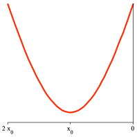
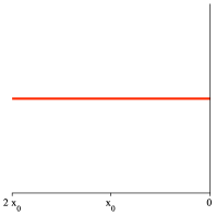
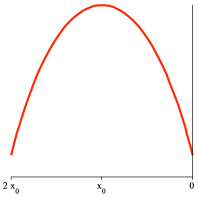
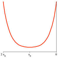
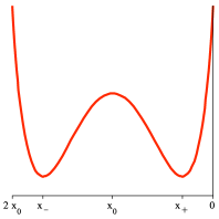
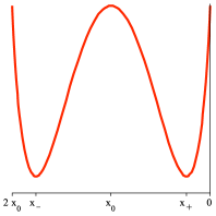
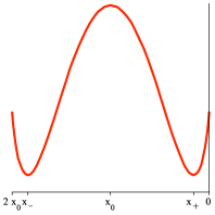
Figure 1: From the left, the function $h_{1,\beta}$ for $\beta<-1$, $\beta=-1$ and $\beta\in(-1,0)$.

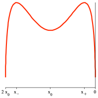
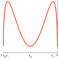
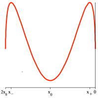
Figure 2: From the left, the function $h_{\alpha,\beta}$, $\alpha>1$, $\beta<0$, for $x_{0}\in[-M_{\alpha,\beta},0)$, $x_{0}\in(-D_{\alpha,\beta},-M_{\alpha,\beta})$, $x_{0}=-D_{\alpha,\beta}$ and $x_{0}<-D_{\alpha,\beta}$.

Figure 3: From the left, the function $h_{\alpha,\beta}$, $\alpha\in(0,1)$, $\beta<0$, for $x_{0}\in[-M_{\alpha,\beta},0)$, $x_{0}\in(-D_{\alpha,\beta},-M_{\alpha,\beta})$, $x_{0}=-D_{\alpha,\beta}$ and $x_{0}<-D_{\alpha,\beta}$.

A detailed analysis of the function $h_{\alpha,\beta}$ then yields the next lemma which we shall prove in Section 5.

Lemma 4.8.

Let $h_{\alpha,\beta}$, $\alpha>0>\beta$, be the positive continuous function defined by $(\ref{4.12})$ and which is even with respect to the line $\{x=x_{0}\}$. i) Let $\alpha=1$. If $\beta\leq-1$ (respectively, $\beta\in(-1,0)$), then $h_{1,\beta}$ is a convex (respectively, concave) function, non decreasing (respectively, decreasing) in the interval $[x_{0},0]$. Therefore, for every $x\in[2x_{0},0]$ we have

$$\hskip-42.67912pt\left\{\!\!\begin{array}[]{lll}|\beta|^{-1/2}|x_{0}|=h_{1,\beta}(x_{0})\leq h_{1,\beta}(x)\leq h_{1,\beta}(0)=|x_{0}|,\quad{\rm if}\ \beta\leq-1\\[5.69054pt] |x_{0}|=h_{1,\beta}(0)\leq h_{1,\beta}(x)\leq h_{1,\beta}(x_{0})=|\beta|^{-1/2}|x_{0}|,\quad{\rm if}\ \beta\in(-1,0).\end{array}\right.$$ (4.52)

ii) Let $\alpha>1$. ii-a) If $x_{0}\in[-M_{\alpha,\beta},0)$, then $h_{\alpha,\beta}$ is a convex function, non decreasing in the interval $[x_{0},0]$. Therefore

$$\hskip-28.45274pt0<|\beta|^{-1}[g_{\alpha,\beta}(x_{0})]^{\alpha}=h_{\alpha,\beta}(x_{0})\leq h_{\alpha,\beta}(x)\leq h_{\alpha,\beta}(0)=|x_{0}|,\quad\forall\,x\in[2x_{0},0].$$ (4.53)

ii-b) If $x_{0}<-M_{\alpha,\beta}$, then

$$\hskip-28.45274pt0<C_{4}(\alpha,\beta,x_{0})\leq h_{\alpha,\beta}(x)\leq C_{5}(\alpha,\beta,x_{0}),\quad\forall\,x\in[2x_{0},0],$$ (4.54)

$C_{j}(\alpha,\beta,x_{0})$, $j=4,5$, being defined by $(\ref{4.37})$ and the first line in $(\ref{4.38})$, respectively. Moreover, there exists a unique inflection point $\widetilde{x}_{\alpha,\beta}\in(x_{0},x_{\alpha,\beta;+})$ such that $h_{\alpha,\beta}$ is convex in $[2x_{0},2x_{0}-\widetilde{x}_{\alpha,\beta}]\cup[\widetilde{x}_{\alpha,\beta},0]$ and concave in $[2x_{0}-\widetilde{x}_{\alpha,\beta},\widetilde{x}_{\alpha,\beta}]$.

iii) Let $\alpha\in(0,1)$. iii-a) If $x_{0}\in[-M_{\alpha,\beta},0)$, then $h_{\alpha,\beta}$ is a concave function, non increasing in the interval $[x_{0},0]$. Therefore

$$\hskip-28.45274pt0<|x_{0}|=h_{\alpha,\beta}(0)\leq h_{\alpha,\beta}(x)\leq h_{\alpha,\beta}(x_{0})=|\beta|^{-1}[g_{\alpha,\beta}(x_{0})]^{\alpha},\quad\forall\,x\in[2x_{0},0].$$ (4.55)

iii-b) If $x_{0}<-M_{\alpha,\beta}$, then

$$\hskip-28.45274pt0<C_{5}(\alpha,\beta,x_{0})\leq h_{\alpha,\beta}(x)\leq C_{4}(\alpha,\beta,x_{0}),\quad\forall\,x\in[2x_{0},0],$$ (4.56)

$C_{j}(\alpha,\beta,x_{0})$, $j=4,5$, being defined by $(\ref{4.37})$ and the second line in $(\ref{4.38})$, respectively. Moreover, there exists a unique inflection point $\overline{x}_{\alpha,\beta}\in(x_{0},x_{\alpha,\beta;+})$ such that $h_{\alpha,\beta}$ is concave in $[2x_{0},2x_{0}-\overline{x}_{\alpha,\beta}]\cup[\overline{x}_{\alpha,\beta},0]$ and convex in $[2x_{0}-\overline{x}_{\alpha,\beta},\overline{x}_{\alpha,\beta}]$.

With the help of Lemma 4.8 we can now find upper and lower bound for the functions $\Theta_{\alpha,\beta}$ and $\Psi_{\alpha,\beta}$ in (4.37). As for Lemma 4.8, the proofs of the forthcoming Corollary 4.10, Lemma 4.13 and Corollary 4.16 will be given in Section 5. In the sequel, $d_{\alpha}$ being defined in (4.34), $E_{\alpha,\beta}$ and $L_{\alpha,\beta}$, $\alpha>0>\beta$, $\alpha\neq 1$, denote the positive numbers

$$\hskip-28.45274ptE_{\alpha,\beta}:=\frac{M_{\alpha,\beta}}{[d_{\alpha}(2-d_{\alpha})]^{1/2}},\qquad L_{\alpha,\beta}:=\frac{D_{\alpha,\beta}}{[d_{\alpha}(2-d_{\alpha})]^{1/2}}.$$

Of course, since $d_{\alpha}\in(5/4,2)$, the numbers $E_{\alpha,\beta}$ and $L_{\alpha,\beta}$ are greater than $M_{\alpha,\beta}$ and $D_{\alpha,\beta}$, respectively. Also, in the case $\alpha\in(0,1)$, it is easy to see that $E_{\alpha,\beta}$ is smaller than $D_{\alpha,\beta}$. In fact, due to (4.38) and (4.39), the inequality $D_{\alpha,\beta}\leq E_{\alpha,\beta}$, $\alpha\in(0,1)$, is equivalent to

$$\hskip-28.45274pt[2^{\alpha}(\alpha+1)^{-\alpha}]^{1/(\alpha-1)}\leq 2^{1/2}(\alpha+1)^{-{1/2}}\alpha^{-(\alpha+1)/[2(\alpha-1)]}[d_{\alpha}(2-d_{\alpha})]^{-1/2},\quad\alpha\in(0,1).$$

Using $d_{\alpha}(2-d_{a})=3(5+2\alpha)/(4+\alpha)^{2}$ and passing to the logarithm, the latter inequality reduces to

$$\mu(\alpha):=\frac{\alpha+1}{1-\alpha}\ln\Big{(}\frac{\alpha+1}{2\alpha}\Big{)}\leq\ln\Big{[}\frac{(4+\alpha)^{2}}{3(5+2\alpha)}\Big{]}=:\nu(\alpha),\quad\alpha\in(0,1).$$ (4.57)

Now, standard computations show that the function $\mu(\alpha)$ on the left-hand side of (4.57) is decreasing in $(0,1)$ and satisfies $\lim_{\alpha\to 0^{+}}\mu(a)=+\infty$ and $\lim_{\alpha\to 1^{-}}\mu(\alpha)=1$, so that $1<\mu(\alpha)$ for every $\alpha\in(0,1)$. On the contrary, the function $\nu(\alpha)$ on the right-hand side of (4.57) is increasing in $(0,1)$, so that $\ln(16/15)=\nu(0)<\nu(\alpha)<\nu(1)=\ln(25/21)$, $\alpha\in(0,1)$. Since $\ln(25/21)<1$, this yields $\nu(\alpha)<\mu(\alpha)$, which contradicts (4.57) and proves $E_{\alpha,\beta}<D_{\alpha,\beta}$, $\alpha\in(0,1)$.

Remark 4.9.

In the case $(\alpha,\beta)=(2,-3/2)$ of the normal Tricomi curve we have $d_{\alpha}=3/2$ and $E_{\alpha,\beta}=1/2$. This suggests that, since (see Remark 4.7) $D_{2,-3/2}=2/3$, the inequality $E_{\alpha,\beta}<D_{\alpha,\beta}$, $\alpha\neq 1$, is satisfied in a real range larger than $\alpha\in(0,1)$. However, in the following we shall not need to know until when the inequality $E_{\alpha,\beta}<D_{\alpha,\beta}$ holds true in the case $\alpha>1$.

We now specified two points of the interval $(2x_{0},0)$ that appear in the upper and lower bounds of the function $\Theta_{\alpha,\beta}$ given in the next Corollary 4.10. For every $\alpha>0$ we set

$$\hskip-28.45274ptx_{\alpha}:=d_{\alpha}x_{0}\in(2x_{0},x_{0}),\qquad\widetilde{x}_{\alpha}:=x_{\alpha}/2\in(x_{0},x_{0}/2).$$ (4.58)

In particular, the function $\theta_{\alpha}$ in (4.34) rewrites as $\theta_{\alpha}(x):=(4+\alpha)x(x-x_{\alpha})$, so it is positive in $[2x_{0},x_{\alpha})$ and negative in $(x_{\alpha},0)$. Observe that, if $x_{0}<-M_{\alpha,\beta}$, then it holds $x_{\alpha}<x_{\alpha,\beta;-}$ or $x_{\alpha,\beta;-}\leq x_{\alpha}$ according to the case $x_{0}\in(-E_{\alpha,\beta},-M_{\alpha,\beta})$ or $x_{0}\leq-E_{\alpha,\beta}$, respectively. Therefore, since in Corollary 4.10 we are interested in the least value of the function $h_{\alpha,\beta}$ in the interval $[2x_{0},x_{\alpha}]$, from Lemma 4.8 we see that the only ambiguous case is $x_{0}<-D_{\alpha,\beta}$, $\alpha\in(0,1)$. (see also Figures 2 and 3). In fact, due to what observed before, if $x_{0}<-D_{\alpha,\beta}$, $\alpha\in(0,1)$, then $x_{0}<-E_{\alpha,\beta}$ and $x_{\alpha}$ belongs to the interval $(x_{\alpha,\beta;-},x_{0})$, in which $h_{\alpha,\beta}$ decreases. Thus, to determine the least value of $h_{\alpha,\beta}$ in $[2x_{0},x_{\alpha}]$ we have to compare the values $h_{\alpha,\beta}(2x_{0})$ and $h_{\alpha,\beta}(x_{\alpha})$. But, if $\alpha\in(0,1)$, then

$$\hskip-28.45274pth_{\alpha,\beta}(x_{\alpha}) \!\!\!=\!\!\! \big{\{}(d_{\alpha}-1)^{2}|x_{0}|^{2}+\beta^{-2}\big{[}(\alpha+1)|\beta|d_{\alpha}(2-d_{\alpha})\big{]}^{2\alpha/(\alpha+1)}|x_{0}|^{4\alpha/(\alpha+1)}\big{\}}^{1/2}{}$$ (4.59)

$$\!\!\!=\!\!\! \big{\{}(d_{\alpha}-1)^{2}|x_{0}|^{-2/\gamma_{\alpha}}+\beta^{-2}\big{[}(\alpha+1)|\beta|d_{\alpha}(2-d_{\alpha})\big{]}^{2\alpha/(\alpha+1)}\big{\}}^{1/2}|x_{0}|^{2\alpha/(\alpha+1)}.$$

where $\gamma_{\alpha}=(\alpha+1)/(\alpha-1)$. Comparing (4.59) with $h_{\alpha,\beta}(2x_{0})=|x_{0}|$, an easy computation shows that

$$\hskip-42.67912pt\min_{\beta<0<\alpha<1}\{h_{\alpha,\beta}(2x_{0}),h_{\alpha,\beta}(x_{\alpha})\}:=\left\{\!\begin{array}[]{lll}h_{\alpha,\beta}(2x_{0}),\quad{\rm if}\ x_{0}\in(-L_{\alpha,\beta},-D_{\alpha,\beta}),\\[5.69054pt] h_{\alpha,\beta}(x_{\alpha})=h_{\alpha,\beta}(2x_{0}),\quad{\rm if}\ x_{0}=-L_{\alpha,\beta},\\[5.69054pt] h_{\alpha,\beta}(x_{\alpha}),\quad{\rm if}\ x_{0}<-L_{\alpha,\beta}.\end{array}\right.$$ (4.63)

Corollary 4.10.

Let $\Theta_{\alpha,\beta}$, $\alpha>0>\beta$, be the function defined in $(\ref{4.29})$ and let $x_{\alpha,\beta;\pm}$, $x_{\alpha}$ and $\widetilde{x}_{\alpha}$ be the points in $(\ref{4.36})$ and $(\ref{4.46})$. i) Let $\alpha=1$. Then

$$\hskip-56.9055ptC_{6}(\beta,x_{0})\leq\Theta_{1,\beta}(x)\leq C_{7}(\beta,x_{0}),\quad\forall\,x\in[2x_{0},0],$$ (4.64)

where

$$\hskip-28.45274pt0>C_{6}(\beta,x_{0}) \!\!\!\!:=\!\!\! \left\{\!\begin{array}[]{lll}[h_{1,\beta}(x_{0})]^{-1}\theta_{1}(\widetilde{x}_{1}),\quad{\rm if}\ \beta\leq-1,\\[5.69054pt] [h_{1,\beta}(0)]^{-1}\theta_{1}(\widetilde{x}_{1}),\quad{\rm if}\ \beta\in(-1,0),\end{array}\right.$$ (4.67)

$$\hskip-28.45274pt0<C_{7}(\beta,x_{0}) \!\!\!\!:=\!\!\! \left\{\!\begin{array}[]{lll}[h_{1,\beta}(x_{1})]^{-1}\theta_{1}(2x_{0}),\quad{\rm if}\ \beta\leq-1,\\[5.69054pt] \Theta_{1,\beta}(2x_{0}),\quad{\rm if}\ \beta\in(-1,0),\end{array}\right.$$ (4.70)

ii) Let $\alpha>1$. Then

$$\hskip-28.45274ptC_{8}(\alpha,\beta,x_{0})\leq\Theta_{\alpha,\beta}(x)\leq C_{9}(\alpha,\beta,x_{0}),\quad\forall\,x\in[2x_{0},0],$$ (4.71)

where

$$\hskip-28.45274pt0>C_{8}(\alpha,\beta,x_{0}) \!\!\!\!:=\!\!\! \left\{\!\begin{array}[]{lll}[h_{\alpha,\beta}(x_{0})]^{-1}\theta_{\alpha}(\widetilde{x}_{\alpha}),\quad{\rm if}\ x_{0}\in[-M_{\alpha,\beta},0),\\[5.69054pt] [h_{\alpha,\beta}(x_{\alpha,\beta;+})]^{-1}\theta_{\alpha}(\widetilde{x}_{\alpha}),\quad{\rm if}\ x_{0}<-M_{\alpha,\beta},\end{array}\right.$$ (4.74)

$$\hskip-28.45274pt0<C_{9}(\alpha,\beta,x_{0}) \!\!\!\!:=\!\!\! \left\{\!\begin{array}[]{lll}[h_{\alpha,\beta}(x_{\alpha})]^{-1}\theta_{\alpha}(2x_{0}),\quad{\rm if}\ x_{0}\in(-E_{\alpha,\beta},0),\\[5.69054pt] [h_{\alpha,\beta}(x_{\alpha,\beta;-})]^{-1}\theta_{\alpha}(2x_{0}),\quad{\rm if}\ x_{0}\leq-E_{\alpha,\beta}.\end{array}\right.$$ (4.77)

iii) Let $\alpha\in(0,1)$. Then

$$\hskip-28.45274ptC_{10}(\alpha,\beta,x_{0})\leq\Theta_{\alpha,\beta}(x)\leq C_{11}(\alpha,\beta,x_{0}),\quad\forall\,x\in[2x_{0},0],$$ (4.78)

where

$$\hskip-14.22636pt0>C_{10}(\alpha,\beta,x_{0}) \!\!\!\!:=\!\!\! \left\{\!\begin{array}[]{lll}[h_{\alpha,\beta}(0)]^{-1}\theta_{\alpha}(\widetilde{x}_{\alpha}),\quad{\rm if}\ x_{0}\in[-D_{\alpha,\beta},0),\\[5.69054pt] [h_{\alpha,\beta}(x_{0})]^{-1}\theta_{\alpha}(\widetilde{x}_{\alpha}),\quad{\rm if}\ x_{0}<-D_{\alpha,\beta},\end{array}\right.$$ (4.81)

$$\hskip-14.22636pt0<C_{11}(\alpha,\beta,x_{0}) \!\!\!\!:=\!\!\! \left\{\!\!\begin{array}[]{lll}\Theta_{\alpha,\beta}(2x_{0}),\quad{\rm if}\ x_{0}\in[-L_{\alpha,\beta},0),\\[5.69054pt] [h_{\alpha,\beta}(x_{\alpha})]^{-1}\theta_{\alpha}(2x_{0}),\quad{\rm if}\ x_{0}<-L_{\alpha,\beta}.\end{array}\right.$$ (4.84)

Remark 4.11.

For the reader’s convenience and to exhibit how they depend on $x_{0}$, we report here the values of the constant $C_{j}(\beta,x_{0})$, $j=6,7$, and $C_{j}(\alpha,\beta,x_{0})$, $j=8,\ldots,11$, in Corollary 4.10. First, observe that $\theta_{\alpha}(2x_{0})=6|x_{0}|^{2}$ for every $\alpha>0$ and recall that $h_{\alpha,\beta}(2x_{0})=h_{\alpha,\beta}(0)=|x_{0}|$ for every $\alpha>0>\beta$. Now, since $d_{1}=7/5$, by evaluating $\theta_{1}(\widetilde{x}_{1})$ and $h_{1,\beta}(x_{1})$ and using $h_{1,\beta}(x_{0})=|\beta|^{-1/2}|x_{0}|$, we find

$$\hskip-28.45274ptC_{6}(\beta,x_{0})=\left\{\!\begin{array}[]{lll}-\displaystyle\frac{49|\beta|^{1/2}|x_{0}|}{20},\quad{\rm if}\ \beta\leq-1,\\[8.53581pt] -\displaystyle\frac{49|x_{0}|}{20},\quad{\rm if}\ \beta\in(-1,0),\end{array}\right.\quad C_{7}(\beta,x_{0})=\left\{\!\begin{array}[]{lll}\displaystyle\frac{30|\beta|^{1/2}|x_{0}|}{[21+4|\beta|]^{1/2}},\quad{\rm if}\ \beta\leq-1,\\[8.53581pt] 6|x_{0}|,\quad{\rm if}\ \beta\in(-1,0).{}\end{array}\right.$$

Instead, when $\alpha>1$ and $C_{4}(\alpha,\beta,x_{0})$ is defined by (4.42), we have

$$\hskip-28.45274ptC_{8}(\alpha,\beta,x_{0})=\left\{\!\begin{array}[]{lll}-c_{8}(\alpha,\beta)|x_{0}|^{2/(\alpha+1)},\quad{\rm if}\ x_{0}\in[-M_{\alpha,\beta},0),\\[5.69054pt] \displaystyle-\frac{(4+\alpha)d_{\alpha}^{2}|x_{0}|^{2}}{4C_{4}(\alpha,\beta,x_{0})},\quad{\rm if}\ x_{0}<-M_{\alpha,\beta},\end{array}\right.$$ (4.91)

$$\hskip-28.45274ptC_{9}(\alpha,\beta,x_{0})=\left\{\!\!\begin{array}[]{lll}c_{9}(\alpha,\beta,x_{0})|x_{0}|,\quad{\rm if}\ x_{0}\in(-E_{\alpha,\beta},0),\\[2.84526pt] \displaystyle\frac{6|x_{0}|^{2}}{C_{4}(\alpha,\beta,x_{0})},\quad{\rm if}\ x_{0}\leq-E_{\alpha,\beta}.\end{array}\right.{}$$ (4.94)

Here

$${}\hskip-14.22636ptc_{8}(\alpha,\beta) \!\!\!\!:=\!\!\! (4+\alpha)|\beta|\big{[}(\alpha+1)|\beta|/2\big{]}^{-\alpha/(\alpha+1)}(d_{\alpha}/2)^{2},$$

$$c_{9}(\alpha,\beta,x_{0}) \!\!\!\!:=\!\!\! 6\big{\{}(d_{\alpha}-1)^{2}+\beta^{-2}\big{[}(\alpha+1)|\beta|d_{\alpha}(2-d_{\alpha})/2\big{]}^{2\alpha/(\alpha+1)}|x_{0}|^{2/\gamma_{\alpha}}\big{\}}^{-1/2},{}$$

where $\gamma_{\alpha}=(\alpha+1)/(\alpha-1)$. Finally, if $\alpha\in(0,1)$, then using (4.59) we obtain

$$\hskip-28.45274ptC_{10}(\alpha,\beta,x_{0})=\left\{\!\!\begin{array}[]{lll}-(4+\alpha)(d_{\alpha}/2)^{2}|x_{0}|,\quad{\rm if}\ x_{0}\in[-D_{\alpha,\beta},0),\\[2.84526pt] -c_{10}(\alpha,\beta)|x_{0}|^{2/(\alpha+1)},\quad{\rm if}\ x_{0}<-D_{\alpha,\beta},\end{array}\right.{}$$ (4.97)

$$\hskip-28.45274ptC_{11}(\alpha,\beta,x_{0})=\left\{\!\!\begin{array}[]{lll}6|x_{0}|,\quad{\rm if}\ x_{0}\in[-L_{\alpha,\beta},0),\\[2.84526pt] c_{11}(\alpha,\beta,x_{0})|x_{0}|^{2/(\alpha+1)},\quad{\rm if}\ x_{0}<-L_{\alpha,\beta},\end{array}\right.{}$$ (4.100)

where $c_{10}(\alpha,\beta)=c_{8}(\alpha,\beta)$ and

$$\hskip-28.45274ptc_{11}(\alpha,\beta,x_{0}):=6\big{\{}(d_{\alpha}-1)^{2}|x_{0}|^{-2/\gamma_{\alpha}}+\beta^{-2}\big{[}(\alpha+1)|\beta|d_{\alpha}(2-d_{\alpha})\big{]}^{2\alpha/(\alpha+1)}\big{\}}^{-1/2}.$$

Remark 4.12.

Notice that, when $x_{0}<-M_{\alpha,\beta}$, one has $x_{\alpha,\beta;+}=\widetilde{x}_{\alpha}$ for $x_{0}=-\widetilde{E}_{\alpha,\beta}$, where $\widetilde{E}_{\alpha,\beta}:=\{d_{\alpha}[1-(d_{\alpha}/4)]\}^{-1/2}M_{\alpha,\beta}>M_{\alpha,\beta}$. In particular, if $d_{\alpha}\in(4/3,2)$, then $\widetilde{E}_{\alpha,\beta}\in(M_{\alpha,\beta},E_{\alpha,\beta})$. Therefore, since $d_{\alpha}\in(4/3,2)$ for every $\alpha>1/2$, when $\alpha>1$ and $x_{0}=-\widetilde{E}_{\alpha,\beta}$ the estimate from below in (4.71) becomes $\Theta_{\alpha,\beta}(x_{\alpha,\beta;+})\leq\Theta_{\alpha,\beta}(x)$, which is sharp. On the contrary, when $x_{0}<-E_{\alpha,\beta}$ is large enough, $x_{\alpha,\beta;+}$ and $x_{\alpha,\beta;-}$ approach $0$ and $2x_{0}$, respectively. This implies that, for $x_{0}<-E_{\alpha,\beta}$ large enough, while the lower bound in (4.71) approaches $[h_{\alpha,\beta}(0)]^{-1}\theta_{\alpha}(\widetilde{x}_{\alpha})\leq\Theta_{\alpha,\beta}(x)$ and becomes less precise, the upper bound approaches $\Theta_{\alpha,\beta}(x)\leq\Theta_{\alpha,\beta}(2x_{0})$ and becomes more accurate.

We now specify some other points which appear in Lemma 4.13 below, where, under the assumption $\alpha\geq 1/2$, we find upper and lower bounds for the function $\Psi_{\alpha,\beta}$ defined in (4.36). For every $\alpha\geq 1/2$ and $\beta<0$ we set

$$\hskip-28.45274pt\overline{x}_{\alpha}:=\frac{(4\alpha+1)x_{0}}{3\alpha},\qquad\overline{x}_{\alpha;\pm}:=x_{0}\pm\Big{(}\frac{\alpha+1}{\alpha+4}\Big{)}^{1/2}|x_{0}|,$$ (4.101)

$$\hskip-28.45274ptx_{\beta;\pm}:=\frac{3x_{0}}{2}\pm\frac{(8+|\beta|^{2}x_{0}^{2})^{1/2}}{2|\beta|},\qquad\widetilde{x}_{\beta;\pm}:=x_{0}\pm\frac{(6+3|\beta|^{2}x_{0}^{2})^{1/2}}{3|\beta|},$$ (4.102)

$$\hskip-28.45274ptx_{\beta}=\frac{2|\beta|x_{0}}{3+2|\beta|},\qquad\widehat{x}_{\beta;\pm}:=\frac{(9+8|\beta|)x_{0}\pm[8(3+2|\beta|)^{2}+9]^{1/2}|x_{0}|}{4(3+2|\beta|)}.$$ (4.103)

Observe that $x_{\beta;-}<2x_{0}$, $x_{\beta;+}>x_{0}$ and $\widetilde{x}_{\beta;-}<x_{0}<\widetilde{x}_{\beta;+}$ for every $\beta<0$, but the points $x_{\beta;+}$, $\widetilde{x}_{\beta;+}$ and $\widetilde{x}_{\beta;-}$ belong to $(x_{0},0)$ and $(2x_{0},x_{0})$, respectively, only if $x_{0}<-|\beta|^{-1}$. Otherwise, if $x_{0}\in[-|\beta|^{-1},0)$, then $x_{\beta;+}\geq 0$, $\widetilde{x}_{\beta;+}\geq 0$ and $\widetilde{x}_{\beta;-}\leq 2x_{0}$. Instead, for every $\alpha\geq 1/2$ and $\beta<0$, it is easy to see that the points $\overline{x}_{\alpha}$, $\overline{x}_{\alpha;\pm}$, $x_{\beta}$ and $\widehat{x}_{\beta;\pm}$ satisfy $\overline{x}_{\alpha}\in[2x_{0},x_{0})$, $\overline{x}_{\alpha;-},\widehat{x}_{\beta;-}\in(2x_{0},x_{0})$ and $\overline{x}_{\alpha;+},x_{\beta},\widehat{x}_{\beta;+}\in(x_{0},0)$, with $x_{\beta}<\widehat{x}_{\beta;+}$.

Finally, for every $\beta<0$ we define the positive number $R_{\beta}$ by

$$\hskip-28.45274ptR_{\beta}:=\frac{(3+2|\beta|)|\beta|^{1/2}}{4[3(3+|\beta|)]^{1/2}}.$$ (4.104)

Since the number $R_{\beta}$ appears in the case $\alpha=2$ of Lemma 4.13, we observe here that $R_{\beta}$ is greater than $M_{2,\beta}=|\beta|/(2\sqrt{3})$ for every $\beta<0$. Also, using $c_{2,\beta}=|\beta|^{2}/12$, an easy computation shows that the point $x_{2,\beta;+}$ defined by (4.41) is related to the point $x_{\beta}$ in (4.103) by $x_{2,\beta;+}<x_{\beta}$ or $x_{\beta}\leq x_{2,\beta;+}$ according to the case $x_{0}\in(-R_{\beta},-M_{2,\beta})$ or $x_{0}\leq-R_{\beta}$.

Lemma 4.13.

Let $\Psi_{\alpha,\beta}$, $\alpha\geq 1/2$, $\beta<0$, be the function defined in $(\ref{4.31})$ and let $x_{\alpha,\beta;\pm}$, $\overline{x}_{\alpha}$, $\overline{x}_{\alpha;\pm}$, $x_{\beta;+}$, $\widetilde{x}_{\beta;\pm}$, $x_{\beta}$ and $\widehat{x}_{\beta;\pm}$ be the points in $(\ref{4.36})$ and $(\ref{4.58})-(\ref{4.60})$. i) Let $\alpha=1/2$. i-a) If $x_{0}\in[-|\beta|^{-1},0)$, then

$$\hskip-28.45274ptC_{12}(\beta,x_{0})\leq\Psi_{1/2,\beta}(x)\leq C_{13}(\beta,x_{0}):=0,\quad\forall\,x\in[2x_{0},0].$$ (4.105)

Here, $D_{1/2,\beta}$ being equal to $(3/4)|\beta|^{-2}$, we have set

$$\hskip-28.45274pt0>C_{12}(\beta,x_{0}):=\left\{\begin{array}[]{lll}\Psi_{1/2,\beta}(2x_{0}),\quad{\rm if}\ \beta\in[-3/4,0),\\[5.69054pt] [h_{1/2,\beta}(x_{0})]^{-1}\psi_{1/2,\beta}(2x_{0}),\quad{\rm if}\ \beta<-3/4,\ x_{0}\in[-|\beta|^{-1},-D_{1/2,\beta}),\\[5.69054pt] \Psi_{1/2,\beta}(2x_{0}),\quad{\rm if}\ \beta<-3/4,\ x_{0}\in[-D_{1/2,\beta},0).\end{array}\right.$$ (4.109)

i-b) Let $x_{0}<-|\beta|^{-1}$. Then

$$\hskip-28.45274ptC_{14}(\beta,x_{0})\leq\Psi_{1/2,\beta}(x)\leq C_{15}(\beta,x_{0}),\quad\forall\,x\in[2x_{0},0],$$ (4.110)

where, $c_{15}(\beta,x_{0})$ standing for $\min\{h_{1/2,\beta}(x_{\beta;+}),h_{1/2,\beta}(0)\}$, we have set

$$\hskip-14.22636pt0>C_{14}(\beta,x_{0}) \!\!\!\!:=\!\!\! \left\{\!\begin{array}[]{lll}[h_{1/2,\beta}(2x_{0})]^{-1}\psi_{1/2,\beta}(\widetilde{x}_{\beta;-}),\quad{\rm if}\ \beta\in(-3/4,0),\ x_{0}\in[-D_{1/2,\beta},-|\beta|^{-1}),\\[5.69054pt] [h_{1/2,\beta}(x_{0})]^{-1}\psi_{1/2,\beta}(\widetilde{x}_{\beta;-}),\quad{\rm if}\ \beta\in(-3/4,0),\ x_{0}<-D_{1/2,\beta},\\[5.69054pt] [h_{1/2,\beta}(x_{0})]^{-1}\psi_{1/2,\beta}(\widetilde{x}_{\beta;-}),\quad{\rm if}\ \beta\leq-3/4,\end{array}\right.$$ (4.114)

$$\hskip-14.22636pt0<C_{15}(\beta,x_{0}) \!\!\!\!:=\!\!\! \left\{\!\begin{array}[]{lll}[h_{1,\beta}(0)]^{-1}\psi_{1/2,\beta}(\widetilde{x}_{\beta;+}),\quad{\rm if}\ \beta\in(-3/4,0),\ x_{0}\in[-D_{1/2,\beta},-|\beta|^{-1}),\\[5.69054pt] [c_{15}(\beta,x_{0})]^{-1}\psi_{1/2,\beta}(\widetilde{x}_{\beta;+}),\quad{\rm if}\ \beta\in(-3/4,0),\ x_{0}<-D_{1/2,\beta},\\[5.69054pt] [c_{15}(\beta,x_{0})]^{-1}\psi_{1/2,\beta}(\widetilde{x}_{\beta;+}),\quad{\rm if}\ \beta\leq-3/4.\end{array}\right.$$ (4.118)

ii) Let $\alpha\in(1/2,1)$. Then

$$\hskip-28.45274ptC_{16}(\alpha,\beta,x_{0})\leq\Psi_{\alpha,\beta}(x)\leq C_{17}(\alpha,\beta,x_{0})\quad\forall\,x\in[2x_{0},0],$$ (4.119)

where

$$\hskip-28.45274pt0>C_{16}(\alpha,\beta,x_{0}) \!\!\!\!:=\!\!\! \left\{\!\begin{array}[]{lll}[h_{\alpha,\beta}(2x_{0})]^{-1}[\varphi_{\alpha,\beta}(\overline{x}_{\alpha})+\phi_{\alpha,\beta}(\overline{x}_{\alpha;-})],\quad{\rm if}\ x_{0}\in[-D_{\alpha,\beta},0),\\[5.69054pt] [h_{\alpha,\beta}(x_{0})]^{-1}[\varphi_{\alpha,\beta}(\overline{x}_{\alpha})+\phi_{\alpha,\beta}(\overline{x}_{\alpha;-})],\quad{\rm if}\ x_{0}<-D_{\alpha,\beta},\end{array}\right.$$ (4.122)

$$0<C_{17}(\alpha,\beta,x_{0}) \!\!\!\!:=\!\!\! \left\{\!\begin{array}[]{lll}[h_{\alpha,\beta}(0)]^{-1}\phi_{\alpha,\beta}(\overline{x}_{\alpha;+}),\quad{\rm if}\ x_{0}\in[-D_{\alpha,\beta},0),\\[5.69054pt] [h_{\alpha,\beta}(x_{0})]^{-1}\phi_{\alpha,\beta}(\overline{x}_{\alpha;+}),\quad{\rm if}\ x_{0}<-D_{\alpha,\beta}.\end{array}\right.$$ (4.125)

iii) Let $\alpha=1$. Then

$$\hskip-28.45274ptC_{18}(\beta,x_{0})\leq\Psi_{1,\beta}(x)\leq C_{19}(\beta,x_{0})\quad\forall\,x\in[2x_{0},0],$$ (4.126)

where

$$\hskip-28.45274pt0>C_{18}(\beta,x_{0}) \!\!\!\!:=\!\!\! \left\{\!\begin{array}[]{lll}[h_{1,\beta}(2x_{0})]^{-1}[\varphi_{1,\beta}(\overline{x}_{1})+\phi_{1,\beta}(\overline{x}_{1;-})],\quad{\rm if}\ \beta\in(-1,0),\\[5.69054pt] [h_{1,\beta}(x_{0})]^{-1}[\varphi_{1,\beta}(\overline{x}_{1})+\phi_{1,\beta}(\overline{x}_{1;-})],\quad{\rm if}\ \beta\leq-1,\end{array}\right.$$ (4.129)

$$0<C_{19}(\beta,x_{0}) \!\!\!\!:=\!\!\! \left\{\!\begin{array}[]{lll}[h_{1,\beta}(0)]^{-1}\phi_{1,\beta}(\overline{x}_{1;+}),\quad{\rm if}\ \beta\in(-1,0),\\[5.69054pt] [h_{1,\beta}(x_{0})]^{-1}\phi_{1,\beta}(\overline{x}_{1;+}),\quad{\rm if}\ \beta\leq-1.\end{array}\right.$$ (4.132)

iv) Let $\alpha\in(1,2)\cup(2,+\infty)$. Then

$$\hskip-14.22636ptC_{20}(\alpha,\beta,x_{0})\leq\Psi_{\alpha,\beta}(x)\leq C_{21}(\alpha,\beta,x_{0})\quad\forall\,x\in[2x_{0},0],$$ (4.133)

where

$$\hskip-28.45274pt0>C_{20}(\alpha,\beta,x_{0}) \!\!\!\!:=\!\!\! \left\{\!\begin{array}[]{lll}[h_{\alpha,\beta}(x_{0})]^{-1}[\varphi_{\alpha,\beta}(\overline{x}_{\alpha})+\phi_{\alpha,\beta}(\overline{x}_{\alpha;-})],\quad{\rm if}\ x_{0}\in[-M_{\alpha,\beta},0),\\[5.69054pt] [h_{\alpha,\beta}(x_{\alpha,\beta;-})]^{-1}[\varphi_{\alpha,\beta}(\overline{x}_{\alpha})+\phi_{\alpha,\beta}(\overline{x}_{\alpha;-})],\quad{\rm if}\ x_{0}<-M_{\alpha,\beta},\end{array}\right.$$ (4.136)

$$0<C_{21}(\alpha,\beta,x_{0}) \!\!\!\!:=\!\!\! \left\{\!\begin{array}[]{lll}[h_{\alpha,\beta}(x_{0})]^{-1}\phi_{\alpha,\beta}(\overline{x}_{\alpha;+}),\quad{\rm if}\ x_{0}\in[-M_{\alpha,\beta},0),\\[5.69054pt] [h_{\alpha,\beta}(x_{\alpha,\beta;+})]^{-1}\phi_{\alpha,\beta}(\overline{x}_{\alpha;+}),\quad{\rm if}\ x_{0}<-M_{\alpha,\beta}.\end{array}\right.$$ (4.139)

v) Let $\alpha=2$. Then

$$\hskip-28.45274ptC_{22}(\beta,x_{0})\leq\Psi_{2,\beta}(x)\leq C_{23}(\beta,x_{0})\quad\forall\,x\in[2x_{0},0],$$ (4.140)

where

$$\hskip-28.45274pt0>C_{22}(\beta,x_{0}) \!\!\!\!:=\!\!\! \left\{\!\begin{array}[]{lll}[h_{2,\beta}(x_{0})]^{-1}\psi_{2,\beta}(\widehat{x}_{\beta;-}),\quad{\rm if}\ x_{0}\in[-M_{2,\beta},0),\\[5.69054pt] [h_{2,\beta}(x_{2,\beta;-})]^{-1}\psi_{2,\beta}(\widehat{x}_{\beta;-}),\quad{\rm if}\ x_{0}<-M_{2,\beta},\end{array}\right.$$ (4.143)

$$\hskip-28.45274pt0<C_{23}(\beta,x_{0}) \!\!\!\!:=\!\!\! \left\{\!\begin{array}[]{lll}[h_{2,\beta}(x_{\beta})]^{-1}\psi_{2,\beta}(\widehat{x}_{\beta;+}),\quad{\rm if}\ x_{0}\in(-R_{\beta},0),\\[5.69054pt] [h_{2,\beta}(x_{2,\beta;+})]^{-1}\psi_{2,\beta}(\widehat{x}_{\beta;+}),\quad{\rm if}\ x_{0}\leq-R_{\beta}.\end{array}\right.$$ (4.146)

Remark 4.14.

From definitions (4.41) and (4.101) we find that the points $x_{\alpha,\beta;+}$ and $\overline{x}_{\alpha;+}$ coincide for $x_{0}=-c(\alpha)M_{\alpha,\beta}<-M_{\alpha,\beta}$, where $c(\alpha)=[(\alpha+4)/3]^{1/2}$, Therefore, if $\alpha\in(1,2)\cup(2,+\infty)$ and $x_{0}=-c(\alpha)M_{\alpha,\beta}$, then the upper bound in (4.133) becomes $\Psi_{\alpha,\beta}(x)\leq\Psi_{\alpha,\beta}(\overline{x}_{\alpha;+})$, $x\in[2x_{0},0]$, which is sharp. Instead, concerning the lower bound in (4.133), we first observe that the points $\overline{x}_{\alpha}$ and $\overline{x}_{\alpha;-}$ coincide only for $\alpha=\widetilde{\alpha}$, where $\widetilde{\alpha}=(5+3\sqrt{1}7)/16$. An easy computation then shows that the equality $x_{\widetilde{\alpha},\beta;-}=\overline{x}_{\widetilde{\alpha};-}$, or, equivalently, $x_{\widetilde{\alpha},\beta;-}=\overline{x}_{\widetilde{\alpha}}$, is satisfied for $x_{0}=-c({\widetilde{\alpha}})M_{\widetilde{\alpha},\beta}<-M_{\widetilde{\alpha},\beta}$, where $c=c(\alpha)$ is as above. As a consequence, if $\alpha=\widetilde{\alpha}\in(1,2)$ and $x_{0}=-c(\widetilde{\alpha})M_{\widetilde{\alpha},\beta}$, then (4.133) reduces to $\Psi_{\widetilde{\alpha},\beta}(\overline{x}_{\widetilde{\alpha};-})\leq\Psi_{\widetilde{\alpha},\beta}(x)\leq\Psi_{\widetilde{\alpha},\beta}(\overline{x}_{\widetilde{\alpha};+})$, $x\in[2x_{0},0]$, which is optimal. On the contrary, if $\alpha\neq\widetilde{\alpha}$ and/or $x_{0}\neq-c(\alpha)M_{\alpha,\beta}$, estimate (4.133) becomes less precise. For instance, when $|x_{0}|>M_{\alpha,\beta}$ is large enough the points $x_{\alpha,\beta;-}$ and $x_{\alpha,\beta;+}$ approach $2x_{0}$ and $0$, respectively, and (4.133) approaches $[h_{\alpha,\beta}(2x_{0})]^{-1}[\varphi_{\alpha,\beta}(\overline{x}_{\alpha})+\phi_{\alpha,\beta}(\overline{x}_{\alpha;-})]\leq\Psi_{\alpha,\beta}(x)\leq[h_{\alpha,\beta}(0)]^{-1}\psi_{\alpha,\beta}(\overline{x}_{\alpha;+})$. Despite of this fact, we want to stress that to find the greatest and least values of $\Psi_{2,\beta}$ using the standard tools of calculus seems a very hard task, due to the difficulties in locating its stationary points (see Remark 5.3).

Remark 4.15.

Similar observations to those in Remark 4.14 hold for $\alpha=2$ and estimate (4.140). In fact, from definitions (4.41) and (4.103) we find that the equalities $x_{2,\beta;-}=\widehat{x}_{\beta;-}$ and $x_{2,\beta;+}=\widehat{x}_{\beta;+}$ are satisfied for $x_{0}=x_{0;-}:=-c_{+}(\beta)M_{2,\beta}$ and $x_{0}=x_{0;+}:=-c_{-}(\beta)M_{2,\beta}$, respectively, where

$$\hskip-28.45274ptc_{\pm}(\beta):=\frac{4(3+2|\beta|)}{\big{\{}\big{(}[8(3+2|\beta|)^{2}+9]^{1/2}\pm 3\big{)}^{2}-36\big{\}}^{1/2}},\quad\beta<0.$$

We get $1<c_{+}(\beta)<c_{-}(\beta)$, so that $x_{0;+}<x_{0;-}<-M_{2,\beta}$ for every $\beta<0$. In addition, using $M_{2,\beta}=|\beta|/(2\sqrt{3})$ and definition (4.104), easy computations yield $x_{0;+}<-R_{\beta}$ for every $\beta<0$, whereas $x_{0;-}<-R_{\beta}$ only for $\beta<\widetilde{\beta}$, where $\widetilde{\beta}=3(1-\sqrt{3})/2$. From (4.140)–(4.146) we thus deduce that, if $x_{0}=x_{0;-}$ (respectively, $x_{0}=x_{0;+}$), then the estimate from below (respectively, above) in (4.140) becomes $\Psi_{2,\beta}(\widehat{x}_{\beta;-})\leq\Psi_{2,\beta}(x)$ (respectively, $\Psi_{2,\beta}(x)\leq\Psi_{2,\beta}(\widehat{x}_{\beta;+}))$, which is sharp. Observe also that in the case $(\alpha,\beta)=(2,-3/2)$, i.e. the case of the normal Tricomi curve, we have $R_{\beta}=1/2$ and, according to $\beta<\widetilde{\beta}$, both the point $x_{0;\pm}$ are less than $-1/2$. Indeed, letting $\beta=-3/2$ in $c_{\pm}(\beta)$ and using $M_{2,-3/2}=\sqrt{3}/4$, we obtain $x_{0;\pm}=-[(15\pm\sqrt{33})/32]^{1/2}$.

Corollary 4.16.

Let $\alpha\geq 1/2$ and $\beta<0$ and let $C_{2m}(\beta,x_{0})$, $m=6,7,9,11$, and $C_{2n}(\alpha,\beta,x_{0})$, $n=8,10$, be the negative constants defined in $(\ref{4.63})$, $(\ref{4.65})$, $(\ref{4.68})$, $(\ref{4.71})$, $(\ref{4.74})$ and $(\ref{4.77})$. Then

$$\hskip-28.45274pt|\Psi_{\alpha,\beta}(x)|\leq C_{24}(\alpha,\beta,x_{0}),\quad\forall\,x\in[2x_{0},0],$$ (4.147)

where

$$\hskip-28.45274ptC_{24}(\alpha,\beta,x_{0}):=\left\{\!\begin{array}[]{lll}|C_{12}(\beta,x_{0})|,\quad{\rm if}\ \alpha=1/2,\ x_{0}\in[-|\beta|^{-1},0),\\[5.69054pt] |C_{14}(\beta,x_{0})|,\quad{\rm if}\ \alpha=1/2,\ x_{0}<-|\beta|^{-1},\\[5.69054pt] |C_{16}(\alpha,\beta,x_{0})|,\quad{\rm if}\ \alpha\in(1/2,1),\\[5.69054pt] |C_{18}(\beta,x_{0})|,\quad{\rm if}\ \alpha=1,\\[5.69054pt] |C_{20}(\alpha,\beta,x_{0})|,\quad{\rm if}\ \alpha\in(1,2)\cup(2,+\infty),\\[5.69054pt] |C_{22}(\beta,x_{0})|,\quad{\rm if}\ \alpha=2.\end{array}\right.$$ (4.154)

Remark 4.17.

As we have done in Remark 4.11 for the constants $C_{j}(\beta,x_{0})$, $j=6,7$, and $C_{j}(\alpha,\beta,x_{0})$, $j=8,\ldots,11$, here we report the values of the constants $|C_{2m}(\beta,x_{0})|$, $m=6,7,9,11$, and $|C_{2n}(\alpha,\beta,x_{0})|$, $n=8,10$. Using the expression of $\psi_{1/2,\beta}$ (see the proof of Lemma 4.13 and Corollary 4.16 in Section 5) we have

$${}\hskip-28.45274pt|C_{12}(\beta,x_{0})| \!\!\!\!:=\!\!\! \left\{\begin{array}[]{lll}12|\beta|^{-1},\quad{\rm if}\ \beta\in[-3/4,0),\\[5.69054pt] 12(3|\beta|/4)^{-1/3}|x_{0}|^{1/3},\quad{\rm if}\ \beta<-3/4,\ x_{0}\in[-|\beta|^{-1},-D_{1/2,\beta}),\\[5.69054pt] 12|\beta|^{-1},\quad{\rm if}\ \beta<-3/4,\ x_{0}\in[-D_{1/2,\beta},0),\end{array}\right.$$ (4.158)

$$\hskip-28.45274pt|C_{14}(\beta,x_{0})| \!\!\!\!:=\!\!\! \left\{\!\begin{array}[]{lll}c_{14}(\beta,x_{0})|x_{0}|^{-1},\quad{\rm if}\ \beta\in(-3/4,0),\ x_{0}\in[-D_{1/2,\beta},-|\beta|^{-1}),\\[5.69054pt] c_{14}(\beta,x_{0})(3|\beta|/4)^{-1/3}|x_{0}|^{-2/3},\quad{\rm if}\ \beta\in(-3/4,0),\ x_{0}<-D_{1/2,\beta},\\[5.69054pt] c_{14}(\beta,x_{0})(3|\beta|/4)^{-1/3}|x_{0}|^{-2/3},\quad{\rm if}\ \beta\leq-3/4,\end{array}\right.{}$$ (4.162)

where $c_{14}(\beta,x_{0})=-\psi_{1/2,\beta}(\widetilde{x}_{\beta;-})$ is given by the first expression in (5.41). Instead, by evaluating $\varphi_{\alpha,\beta}(\overline{x}_{\alpha})$ and $\phi_{\alpha,\beta}(\overline{x}_{\alpha;-})$, $\alpha>1/2$, $\beta<0$, we get

$${}\hskip-28.45274pt|C_{16}(\alpha,\beta,x_{0})| \!\!\!\!:=\!\!\! \left\{\!\begin{array}[]{lll}c_{1}(\alpha,\beta)|x_{0}|^{(2\alpha-1)/(\alpha+1)}+c_{2}(\alpha,\beta)|x_{0}|^{3/(\alpha+1)},\quad{\rm if}\ x_{0}\in[-D_{\alpha,\beta},0),\\[5.69054pt] c_{3}(\alpha,\beta)|x_{0}|^{\alpha/(\alpha+1)}+c_{4}(\alpha,\beta)|x_{0}|^{(4-\alpha)/(\alpha+1)},\quad{\rm if}\ x_{0}<-D_{\alpha,\beta},\end{array}\right.$$ (4.165)

$$|C_{18}(\beta,x_{0})| \!\!\!\!:=\!\!\! \left\{\!\begin{array}[]{lll}c_{1}(1,\beta)|x_{0}|^{1/2}+c_{2}(1,\beta)|x_{0}|^{3/2},\quad{\rm if}\ \beta\in(-1,0),\\[5.69054pt] c_{3}(1,\beta)|x_{0}|^{1/2}+c_{4}(\alpha,\beta)|x_{0}|^{3/2},\quad{\rm if}\ \beta\leq-1,\end{array}\right.{}$$ (4.168)

$$|C_{20}(\alpha,\beta,x_{0})| \!\!\!\!:=\!\!\! \left\{\!\begin{array}[]{lll}c_{3}(\alpha,\beta)|x_{0}|^{\alpha/(\alpha+1)}+c_{4}(\alpha,\beta)|x_{0}|^{(4-\alpha)/(\alpha+1)},\quad{\rm if}\ x_{0}\in[-M_{\alpha,\beta},0),\\[5.69054pt] c_{5}(\alpha,\beta,x_{0})|x_{0}|^{3\alpha/(\alpha+1)}+c_{6}(\alpha,\beta,x_{0})|x_{0}|^{(\alpha+4)/(\alpha+1)},\quad{\rm if}\ x_{0}<-M_{\alpha,\beta}.\end{array}\right.{}$$ (4.171)

Here, for every $\alpha>1/2$ and $\beta<0$ we have set

$$\hskip-28.45274ptc_{1}(\alpha,\beta):=2\alpha^{-1}(4\alpha+1)^{(4\alpha+1)/(2\alpha+2)}\big{[}(2\alpha^{2}+\alpha-1)/(18\alpha^{2})\big{]}^{(2\alpha-1)/(2\alpha+2)}|\beta|^{-3/(2\alpha+2)},{}$$

$$\hskip-28.45274ptc_{2}(\alpha,\beta):=4\big{[}(\alpha+1)/(\alpha+4)\big{]}^{(\alpha+4)/(2\alpha+2)}(3|\beta|/2)^{3/(2\alpha+2)},{}$$

$$\hskip-28.45274ptc_{j}(\alpha,\beta):=|\beta|\big{[}(\alpha+1)|\beta|/2\big{]}^{-\alpha/(\alpha+1)}c_{j-2}(\alpha,\beta),\quad j=3,4,{}$$

$$\hskip-28.45274ptc_{j}(\alpha,\beta,x_{0}):=[C_{4}(\alpha,\beta,x_{0})]^{-1}c_{j-4}(\alpha,\beta),\quad j=5,6,{}$$

where $C_{4}(\alpha,\beta,x_{0})$ is defined by (4.42). Finally, if $\alpha=2$, then using the first expression in the following (5.46) and evaluating $[g_{2,\beta}(\widehat{x}_{\beta;-})]^{3/2}$ we obtain

$${}\hskip-28.45274pt|C_{22}(\beta,x_{0})| \!\!\!\!:=\!\!\! \left\{\!\begin{array}[]{lll}(4|\beta|/9)^{1/3}c_{7}(\beta)|x_{0}|^{2/3},\quad{\rm if}\ x_{0}\in[-M_{2,\beta},0),\\[5.69054pt] [C_{4}(2,\beta,x_{0})]^{-1}c_{7}(\beta)|x_{0}|^{2}\quad{\rm if}\ x_{0}<-M_{2,\beta},\end{array}\right.$$ (4.174)

where for every $\beta<0$ we have set

$${}\hskip 0.0ptc_{7}(\beta) \!\!\!\!:=\!\!\! (3|\beta|^{-1}/8)^{1/2}[4(3+2|\beta|)]^{-1}\big{\{}[8(3+2|\beta|)^{2}+9]^{1/2}+9\big{\}}{}$$

$$\hskip 28.45274pt\times\big{\{}32|\beta|^{2}+96|\beta|+54+6[8(3+2|\beta|)^{2}+9]^{1/2}\big{\}}^{1/2}.{}$$

For instance, if we let $\beta=-3/2$ in the previous formula of $C_{22}(\beta,x_{0})$, then we obtain the constant $C(x_{0}):=|C_{22}(-3/2,x_{0})|$ for the case when $\sigma_{\alpha,\beta}$ is the normal Tricomi curve. An easy computation shows that this constant is precisely

$${}C(x_{0}) \!\!\!\!:=\!\!\! \left\{\!\begin{array}[]{lll}2^{-19/6}3^{2/3}(3+\sqrt{33})(15+\sqrt{33})^{1/2}|x_{0}|^{2/3},\quad{\rm if}\ x_{0}\in[-\sqrt{3}/4,0),\\[5.69054pt] 2^{-7/2}3[x_{0}^{2}-(3/64)]^{-1/2}(3+\sqrt{33})(15+\sqrt{33})^{1/2}|x_{0}|^{2},\quad{\rm if}\ x_{0}<-\sqrt{3}/4.\end{array}\right.$$ (4.177)

We can now finally proceed to estimate the line integral $\int_{\sigma}\omega_{1}\,{\rm d}s$ in the case when $\sigma=\sigma_{\alpha,\beta}$ for some $\alpha\geq 1/2$ and $\beta<0$. Due to Corollaries 4.10 and 4.16 our estimate will deeply depend on the values of the parameter pair $(\alpha,\beta)$ and the length of the parabolic diameter $|AB|=2|x_{0}|$ of $\Omega_{\alpha,\beta}$.

Lemma 4.18.

Let $\Omega=\Omega_{\alpha,\beta}$ for some $\alpha\geq 1/2$ and $\beta<0$ and let $u$ be a real valued solution of problem $(\ref{3.1})$ which is Fréchet differentiable at each of the points of $\sigma=\sigma_{\alpha,\beta}$ and such that $|y|^{1/2}u_{x}$, $u_{y}\in L^{2}(\sigma)$. Let $\omega_{1}$ be defined by $(\ref{3.9})$. Then, for every $\varepsilon>0$, the following estimate holds:

$$\hskip-42.67912pt0\leq\int_{\sigma}\omega_{1}\,{\rm d}s\leq C_{25}(\alpha,\beta,x_{0},\varepsilon)\||y|^{1/2}u_{x}\|_{L^{2}(\sigma)}^{2}+C_{26}(\alpha,\beta,x_{0},\varepsilon)\|u_{y}\|_{L^{2}(\sigma)}^{2}.$$ (4.178)

Here, for $j=25,26$ we have set

$$\hskip-28.45274ptC_{j}(\alpha,\beta,x_{0},\varepsilon):=\left\{\!\!\begin{array}[]{lll}(-1)^{j+1}C_{k_{1,j}}(1/2,\beta,x_{0})+(\varepsilon/2)|C_{12}(\beta,x_{0})|,\quad{\rm if}\ \alpha=1/2,\ x_{0}\in[-|\beta|^{-1},0),\\[5.69054pt] (-1)^{j+1}C_{k_{1,j}}(1/2,\beta,x_{0})+(\varepsilon/2)|C_{14}(\beta,x_{0})|,\quad{\rm if}\ \alpha=1/2,\ x_{0}<-|\beta|^{-1},\\[5.69054pt] (-1)^{j+1}C_{k_{1,j}}(\alpha,\beta,x_{0})+(\varepsilon/2)|C_{16}(\alpha,\beta,x_{0})|,\quad{\rm if}\ \alpha\in(1/2,1),\\[5.69054pt] (-1)^{j+1}C_{k_{2,j}}(\beta,x_{0})+(\varepsilon/2)|C_{18}(\beta,x_{0})|,\quad{\rm if}\ \alpha=1,\\[5.69054pt] (-1)^{j+1}C_{k_{3,j}}(\alpha,\beta,x_{0})+(\varepsilon/2)|C_{20}(\alpha,\beta,x_{0})|,\quad{\rm if}\ \alpha\in(1,2)\cup(2,+\infty),\\[5.69054pt] (-1)^{j+1}C_{k_{3,j}}(2,\beta,x_{0})+(\varepsilon/2)|C_{22}(\beta,x_{0})|,\quad{\rm if}\ \alpha=2,\end{array}\right.$$ (4.185)

where

$$\hskip-28.45274ptk_{1,j}=\left\{\!\begin{array}[]{lll}11,\quad{\rm if}\ j=25,\\[2.84526pt] 10,\quad{\rm if}\ j=26,\end{array}\right.\quad k_{2,j}=\left\{\!\begin{array}[]{lll}7,\quad{\rm if}\ j=25,\\[2.84526pt] 6,\quad{\rm if}\ j=26,\end{array}\right.\quad k_{3,j}=\left\{\!\begin{array}[]{lll}9,\quad{\rm if}\ j=25,\\[2.84526pt] 8,\quad{\rm if}\ j=26,\end{array}\right.$$ (4.192)

and the constants $C_{m}(\beta,x_{0})$, $m=6,7,12,14,18,22$, and $C_{j}(\alpha,\beta,x_{0})$, $j=8,9,10,11,16,20$, are defined by $(\ref{4.50})$, $(\ref{4.51})$, $(\ref{4.53})$, $(\ref{4.54})$, $(\ref{4.56})$, $(\ref{4.57})$, $(\ref{4.63})$, $(\ref{4.65})$, $(\ref{4.68})$, $(\ref{4.71})$, $(\ref{4.74})$ and $(\ref{4.77})$.

Proof.

First, since $u_{|\sigma_{\alpha,\beta}}=0$, the assumption that $u$ is Fréchet differentiable at each of the points of $\sigma_{\alpha,\beta}$ implies that the directional derivative of $u$ is zero along $\sigma_{\alpha,\beta}$. Therefore, since the assumption $\alpha\geq 1/2$ implies that $\partial\Omega_{\alpha,\beta}$ is $D$-starlike with respect to $D=-3x\partial_{x}-2y\partial_{y}$ (see Lemma 4.2), we are in position to apply the argument in [24, p. 416], to which we refer the reader for the details, to derive the lower bound $0\leq\int_{\sigma}\omega_{1}\,{\rm d}s$. Now, recall that (see formula (4.37))

$$\widehat{\omega_{1}}=\Theta_{\alpha,\beta}(x)y\widehat{u_{x}}^{2}+\Psi_{\alpha,\beta}(x)y^{1/2}\widehat{u_{x}}\,\widehat{u_{y}}-\Theta_{\alpha,\beta}(x)\widehat{u_{y}}^{2},$$ (4.193)

where $\Theta_{\alpha,\beta}$ and $\Psi_{\alpha,\beta}$ are the functions defined in (4.34) and (4.36). Then, using the inequality $2|a||b|\leq\varepsilon a^{2}+\varepsilon^{-1}b^{2}$, $a,b\in{\bf R}$, $\varepsilon>0$, from (4.193) we obtain:

$$\hskip-28.45274pt\widehat{\omega_{1}} \!\!\!\leq\!\!\! \Theta_{\alpha,\beta}(x)y\widehat{u_{x}}^{2}+|\Psi_{\alpha,\beta}(x)||y^{1/2}\widehat{u_{x}}||\widehat{u_{y}}|-\Theta_{\alpha,\beta}(x)\widehat{u_{y}}^{2}{}$$ (4.194)

$$\!\!\!\leq\!\!\! \{\Theta_{\alpha,\beta}(x)+(\varepsilon/2)|\Psi_{\alpha,\beta}(x)|\}y\widehat{u_{x}}^{2}+\{(2\varepsilon)^{-1}|\Psi_{\alpha,\beta}(x)|-\Theta_{\alpha,\beta}(x)\}\widehat{u_{y}}^{2}.$$

It thus now suffices to apply Corollaries 4.10 and 4.16 to conclude the proof. Indeed, due to (4.64)–(4.84), (4.147) and (4.154) inequality (4.194) leads us to

$$\hskip-56.9055pt\widehat{\omega_{1}}\leq C_{25}(\alpha,\beta,x_{0},\varepsilon)y\widehat{u_{x}}^{2}+C_{26}(\alpha,\beta,x_{0},\varepsilon)\widehat{u_{y}}^{2},\quad\forall\,\varepsilon>0,$$

where the constants $C_{j}(\alpha,\beta,x_{0},\varepsilon)$, $j=25,26$, are defined by (4.185), (4.192). Hence

$$\hskip-28.45274pt\int_{\sigma}\omega_{1}\,{\rm d}s\leq C_{25}(\alpha,\beta,x_{0},\varepsilon)\||y|^{1/2}u_{x}\|_{L^{2}(\sigma)}^{2}+C_{26}(\alpha,\beta,x_{0},\varepsilon)\|u_{y}\|_{L^{2}(\sigma)}^{2},\quad\forall\,\varepsilon>0,$$

and the proof of (4.178) is complete. ∎

Remark 4.19.

Notice that the assumption that $u$ is Fréchet differentiable at each of the points of $\sigma$ is necessary only in order to show the estimate from below $0\leq\int_{\sigma}\omega_{1}\,{\rm d}s$, but does not contribute in any way for showing the estimate from above of $\int_{\sigma}\omega_{1}\,{\rm d}s$. Moreover, not even the $D$-starlikeness of $\Omega_{\alpha,\beta}$, which derives from the assumption $\alpha\geq 1/2$, plays any role in the proof of the upper bound of $\int_{\sigma}\omega_{1}\,{\rm d}s$. Indeed, what really counts in the proof of such an upper bound is only the assumption $\alpha\geq 1/2$ which allows us to apply Corollary 4.21.

We can now prove our main result. For brevity, in Theorem 4.20 below, the symbols $L^{2}(\Omega)$, $C^{1}(\overline{\Omega})$ and $C^{2}(\Omega)$ are used without exception for both real and complex valued functions. Needless to say, if we have to deal with complex valued functions, then $L^{2}(\Omega)$ is understood endowed with the usual complex inner product $\langle\cdot,\cdot\rangle_{2,\sim}$ defined in Remark 3.5, whereas the spaces $C^{1}(\overline{\Omega})$ and $C^{2}(\Omega)$ are meant for $C^{1}(\overline{\Omega};{\bf C})$ and $C^{2}(\Omega;{\bf C})$, respectively.

Theorem 4.20.

Let $\Omega=\Omega_{\alpha,\beta}$ for some $\alpha\geq 1/2$ and $\beta<0$ and let $\lambda_{0}>0$ be the principal eigenvalue of $\widetilde{T}_{AC\cup\sigma}$ defined in Theorem 2.4, where $\sigma=\sigma_{\alpha,\beta}$. Let $u=\Re u+i\Im u$, where $\Re u,\Im u\in\widetilde{W}_{AC\cup\sigma}^{1}(\Omega)$, be a non almost everywhere vanishing solution to problem

$$\hskip-14.22636pt\left\{\!\!\begin{array}[]{lll}Tu=\lambda u\quad{\rm in}\ \Omega,\\[5.69054pt] u=0\quad{\rm on}\ AC\cup\sigma,\end{array}\right.\quad\lambda\in[\lambda_{0},+\infty),$$ (4.197)

and assume that $u_{y}$, $xu_{x}$, $yu_{x}\in C^{1}(\overline{\Omega})$, $xu\in C^{2}(\Omega)$, $u\in L^{2}(BC)$ and $|y|^{1/2}u_{x}$, $u_{y}\in L^{2}(BC)\cap L^{2}(\sigma)$. Then, for every $\varepsilon_{j}>0$, $j=1,2$, the following estimate holds:

$$\hskip 0.0pt0 \!\!\!<\!\!\! 2\lambda^{1/2}\|u\|_{L^{2}(\Omega)}{}$$ (4.198)

$$\!\!\!\leq\!\!\! \Big{\{}C_{1}(x_{0},\varepsilon_{1})\||y|^{1/2}u_{x}\|_{L^{2}(BC)}^{2}+C_{2}(x_{0},\varepsilon_{1})\|u_{y}\|_{L^{2}(BC)}^{2}{}$$

$$\ \,+\,C_{3}(x_{0})\big{[}\|\Re u\|_{L^{2}(BC)}+\|\Im u\|_{L^{2}(BC)}\big{]}\big{[}\||y|^{1/2}u_{x}\|_{L^{2}(BC)}+\|u_{y}\|_{L^{2}(BC)}\big{]}{}$$

$$\ \,+\,C_{25}(\alpha,\beta,x_{0},\varepsilon_{2})\||y|^{1/2}u_{x}\|_{L^{2}(\sigma)}^{2}+C_{26}(\alpha,\beta,x_{0},\varepsilon_{2})\|u_{y}\|_{L^{2}(\sigma)}^{2}\Big{\}}^{1/2},$$

where $C_{j}(x_{0},\varepsilon_{1})$, $j=1,2$, are defined by $(\ref{4.20})$ with $\varepsilon=\varepsilon_{1}$, $C_{3}(x_{0})$ is defined by $(\ref{4.25})$, and $C_{j}(\alpha,\beta,x_{0},\varepsilon_{2})$, $j=25,26$, are defined by $(\ref{4.82})$, $(\ref{4.83})$ with $\varepsilon=\varepsilon_{2}$.

Proof.

First (see (3.17)), since $\lambda\in[\lambda_{0},+\infty)$ and $u$ does not vanish almost everywhere, we have that the real valued functions $v_{1}=\Re u$ and $v_{2}=\Im u$ also solve (4.197), and that at least one of the two is not the zero element of $L^{2}(\Omega)$. Moreover, our assumptions on $u$ imply that $(v_{j})_{y}$, $x(v_{j})_{x}$, $y(v_{j})_{x}\in C^{1}(\overline{\Omega})$, $xv_{j}\in C^{2}(\Omega)$, $v_{j}\in L^{2}(BC)$ and $|y|^{1/2}(v_{j})_{x}$, $(v_{j})_{y}\in L^{2}(BC)\cap L^{2}(\sigma)$, $j=1,2$. Thus, setting $f(t)=\lambda t$, $t\in{\bf R}$, we may as well suppose from the outset that $u\in\widetilde{W}^{1}_{AC\cup\sigma}(\Omega)$, $u\neq 0$, is a real valued solution to problem (3.3) satisfying the assumptions of Theorem 3.3 and Lemmas 4.4, 4.5 and 4.18. Observe that, according to Remark 4.19, here we do not require that $u$ is Fréchet differentiable at each of the points of $\sigma$, since we do not need the lower bound $0\leq\int_{\sigma}\omega_{1}\displaystyle$. In particular, $u$ satisfies the identity (3.12) with $F(t)=(\lambda/2)t^{2}$, $t\in{\bf R}$. Therefore, since $10F(u)-uf(u)=4\lambda u^{2}$, we have

$$\hskip-56.9055pt0<4\lambda\|u\|_{L^{2}(\Omega)}^{2}=\int_{BC}(\omega_{1}+\omega_{2})\,{\rm d}s+\int_{\sigma}\omega_{1}\,{\rm d}s,$$ (4.199)

where $\omega_{1}$ and $\omega_{2}$ are defined by (3.13) and (3.14). Hence, taking $\varepsilon=\varepsilon_{1}>0$ in Lemma 4.4 and $\varepsilon=\varepsilon_{2}>0$ in Lemma 4.18 and applying estimate (4.24), (4.29) and (4.178), from (4.199) we deduce

$$\hskip 0.0pt0<4\lambda\|u\|_{L^{2}(\Omega)}^{2} \!\!\!\leq\!\!\! C_{1}(x_{0},\varepsilon_{1})\||y|^{1/2}u_{x}\|_{L^{2}(BC)}^{2}+C_{2}(x_{0},\varepsilon_{1})\|u_{y}\|_{L^{2}(BC)}^{2}{}$$ (4.200)

$$+\,C_{3}(x_{0})\|u\|_{L^{2}(BC)}\big{[}\||y|^{1/2}u_{x}\|_{L^{2}(BC)}+\|u_{y}\|_{L^{2}(BC)}\big{]}{}$$

$$+\,C_{25}(\alpha,\beta,x_{0},\varepsilon_{2})\||y|^{1/2}u_{x}\|_{L^{2}(\sigma)}^{2}+C_{26}(\alpha,\beta,x_{0},\varepsilon_{2})\|u_{y}\|_{L^{2}(\sigma)}^{2}.$$

This proves (4.198) in the case that $u$ is real valued. To complete the proof in the general case it suffices to replace $u$ in (4.200) with $\Re u$ and $\Im u$, respectively, and then summing up the so obtained estimate, taking into account the identities $|y|^{1/2}({\mathfrak{F}}u)_{x}={\mathfrak{F}}(|y|^{1/2}u_{x})$ and $({\mathfrak{F}}u)_{y}={\mathfrak{F}}(u_{y})$, ${\mathfrak{F}}=\Re,\Im$, and the inequalities $\||y|^{1/2}(\mathfrak{F}u)_{x}\|_{L^{2}(BC)}\leq\||y|^{1/2}u_{x}\|_{L^{2}(BC)}$ and $\|(\mathfrak{F}u)_{y}\|_{L^{2}(BC)}\leq\|u_{y}\|_{L^{2}(BC)}$, ${\mathfrak{F}}=\Re,\Im$. ∎

Remark 4.21.

Notice that, if $u\in\widetilde{W}_{AC\cup\sigma}^{1}$ is an eigenfunction corresponding to an eigenvalue $\lambda\in[\lambda_{0},+\infty)$ satisfying the assumption of Theorem 4.20, then (4.199) improves the inequality $0\leq\int_{BC}(\omega_{1}+\omega_{2})\,{\rm d}s+\int_{\sigma}\omega_{1}\,{\rm d}s$ which is shown in the proof of [24, Theorem 4.2] (take there $k=0$) under the assumption $u\in C^{2}(\overline{\Omega})$.

Of course, when $\Omega=\Omega_{\alpha,\beta}$ for some $\alpha\geq 1/2$ and $\beta<0$, one can apply estimate (4.198), with the quadruplet $(\lambda,u,\Re u,\Im u)$ being replaced by $(\lambda_{0},u_{0},u_{0},0)$ and $(\widetilde{\lambda}_{0},\widetilde{u}_{0},\widetilde{u}_{0},0)$, respectively, to the eigenfunctions $u_{0}\in\widetilde{W}_{AC\cup\sigma}(\Omega)$ and $\widetilde{u}_{0}\in\widetilde{W}_{AC\cup\sigma}(\Omega)\cap C(\overline{\Omega})$ of Theorems 2.4 and 2.5, provided one can show that they satisfy the additional regularity requirements of Theorem 4.20.

5 Proof of Lemmas 4.8 and 4.13 and Corollaries 4.10 and 4.16

Proof of Lemma 4.8. First, from definitions (4.3) and (4.15) we immediately derive $h_{\alpha,\beta}(x)=h_{\alpha,\beta}(2x_{0}-x)$, so $h_{\alpha,\beta}$ is an even function with respect to the line $\{x=x_{0}\}$ and it suffices to prove the lemma assuming $x\in[x_{0},0]$. With such a convention, we change the variable from $x$ to $X=x-x_{0}\in[0,-x_{0}]$ and we consider the function

$$\hskip-28.45274ptH_{\alpha,\beta}(X):=h_{\alpha,\beta}(X+x_{0})=\big{\{}X^{2}+\beta^{-2}[G_{\alpha,\beta}(X)]^{2\alpha}\big{\}}^{1/2},\quad X\in[0,-x_{0}],$$ (5.1)

where

$$\hskip-28.45274ptG_{\alpha,\beta}(X):=g_{\alpha,\beta}(X+x_{0})=\bigg{[}\frac{(\alpha+1)|\beta|(x_{0}^{2}-X^{2})}{2}\bigg{]}^{1/(\alpha+1)},\quad X\in[0,-x_{0}].$$ (5.2)

Differentiating (5.1) with respect to $X$ and using $G_{\alpha,\beta}^{\prime}(X)=\beta X[G_{\alpha,\beta}(X)]^{-\alpha}$, $X\in[0,-x_{0})$, we get

$$\hskip-28.45274ptH_{\alpha,\beta}^{\prime}(X)=[H_{\alpha,\beta}(X)]^{-1}X\big{\{}1-\alpha|\beta|^{-1}[G_{\alpha,\beta}(X)]^{\alpha-1}\big{\}},\quad X\in[0,-x_{0}).$$ (5.3)

Hence, the three cases $\alpha=1$, $\alpha>1$ and $\alpha\in(0,1)$ have to be considered.

i) Case $\alpha=1$. In this case $H_{1,\beta}^{\prime}(X)\geq 0$ if and only if $1-|\beta|^{-1}\geq 0$, i.e. if $\beta\leq-1$. In particular, if $\beta=-1$, then $H_{1,\beta}^{\prime}(X)=0$ for every $X\in[0,-x_{0})$ and (see the observation below formula (4.15)) $H_{1,\beta}(X)$ is costant equal to $|x_{0}|$. Therefore $H_{1,\beta}$ is non decreasing (respectively, decreasing) for $\beta\leq-1$ (respectively, $\beta\in(-1,0)$) and (4.52) follows from

$${}\left\{\!\begin{array}[]{lll}h_{1,\beta}(x_{0})=H_{1,\beta}(0)\leq H_{1,\beta}(X)\leq H_{1,\beta}(-x_{0})=h_{1,\beta}(0),\quad\beta\leq-1,\\[5.69054pt] h_{1,\beta}(0)=H_{1,\beta}(-x_{0})\leq H_{1,\beta}(X)\leq H_{1,\beta}(0)=h_{1,\beta}(x_{0}),\quad\beta\in(-1,0).\end{array}\right.$$ (5.6)

To complete the proof of the case $\alpha=1$, we rewrite (5.3) as $H_{1,\beta}^{\prime}(X)=(1-|\beta|^{-1})\widetilde{H}_{1,\beta}(X)$, where $\widetilde{H}_{1,\beta}(X)$ is the nonnegative function $[H_{1,\beta}(X)]^{-1}X$, $X\in[0,-x_{0})$. Differentiating $\widetilde{H}_{1,\beta}(X)$ with respect to $X$ and using (5.1)–(5.3) with $\alpha=1$, we get that $\widetilde{H}_{1,\beta}$ is an increasing function, since

$${}\hskip-28.45274pt\widetilde{H}_{1,\beta}^{\prime}(X) \!\!\!=\!\!\! [H_{1,\beta}(X)]^{-3}\big{\{}[H_{1,\beta}(X)]^{2}-(1-|\beta|^{-1})X^{2}\big{\}}{}$$

$$\!\!\!=\!\!\! [H_{1,\beta}(X)]^{-3}|\beta|^{-1}x_{0}^{2}>0,\quad\forall\,X\in[0,-x_{0}).{}$$

As a consequence, if $\beta<-1$, then $1-|\beta|^{-1}>0$, and $H_{1,\beta}^{\prime}(X)=(1-|\beta|^{-1})\widetilde{H}_{1,\beta}(X)$ is increasing too, proving the convexity of $h_{1,\beta}(x)$, $x\in[2x_{0},0]$. On the contrary, if $\beta\in(-1,0)$, then $1-|\beta|^{-1}<0$ and $H_{1,\beta}^{\prime}(X)=(1-|\beta|^{-1})\widetilde{H}_{1,\beta}(X)$ turns out to be a decreasing function, proving the concavity of $h_{1,\beta}(x)$, $x\in[2x_{0},0]$.

ii) Case $\alpha>1$. In this case from (5.3) we find $H_{\alpha,\beta}^{\prime}(X)\geq 0$ if and only if $1-\alpha|\beta|^{-1}[G_{\alpha,\beta}(X)]^{\alpha-1}\geq 0$, i.e. if and only if $[G_{\alpha,\beta}(X)]^{\alpha-1}\leq\alpha^{-1}|\beta|$. Raising both sides of this latter inequality to the power $\gamma_{\alpha}=(\alpha+1)/(\alpha-1)>1$ and using (5.2) we thus find $H_{\alpha,\beta}^{\prime}(X)\geq 0$ if and only if $X^{2}\geq x_{0}^{2}-c_{\alpha,\beta}$, where $c_{\alpha,\beta}$ is defined by (4.38). Therefore, if $x_{0}\in[-M_{\alpha,\beta},0)$, $M_{\alpha,\beta}=(c_{\alpha,\beta})^{1/2}$, then $H_{\alpha,\beta}^{\prime}(X)\geq 0$ for every $X\in[0,-x_{0})$ and $H_{\alpha,\beta}$ is a non decreasing function in $[0,-x_{0}]$. Hence, (4.53) follows from $h_{\alpha,\beta}(x_{0})=H_{\alpha,\beta}(0)\leq H_{\alpha,\beta}(X)\leq H_{\alpha,\beta}(-x_{0})=h_{\alpha,\beta}(0)$. On the contrary, if $x_{0}<-M_{\alpha,\beta}$, we have $H_{\alpha,\beta}^{\prime}(X)\leq 0$ in $[0,X_{\alpha,\beta;+}]$ and $H_{\alpha,\beta}^{\prime}(X)\geq 0$ in $[X_{\alpha,\beta;+},-x_{0})$, where $X_{\alpha,\beta;+}={[x_{0}^{2}-c_{\alpha,\beta}]}^{1/2}$. Hence $H_{\alpha,\beta}$ is non increasing in $[0,X_{\alpha,\beta;+}]$ and non decreasing in $[X_{\alpha,\beta;+},-x_{0})$, and (4.54) follows from $h_{\alpha,\beta}(x_{\alpha,\beta;+})=H_{\alpha,\beta}(X_{\alpha,\beta;+})\leq H_{\alpha,\beta}(X)\leq\max\{H_{\alpha,\beta}(0),H_{\alpha,\beta}(-x_{0})\}=\max\{h_{\alpha,\beta}(x_{0}),h_{\alpha,\beta}(0)\}$. To complete the proof of the case $\alpha>1$, let us assume first $x_{0}\in[-M_{\alpha,\beta},0)$. As we noted above, in such a case the function $\widetilde{G}_{\alpha,\beta}(X):=1-\alpha|\beta|^{-1}[G_{\alpha,\beta}(X)]^{\alpha-1}$, $X\in[0,-x_{0})$, is nonnegative and, moreover, is non decreasing due to the non increasing character of $G_{\alpha,\beta}$. An easy computations, taking into account formulae (5.1) and (5.3), shows that the nonnegative function $\widetilde{H}_{\alpha,\beta}(X):=[H_{\alpha,\beta}(X)]^{-1}X$, $X\in[0,-x_{0})$, is non decreasing too, since for every $X\in[0,-x_{0})$ we have

$$\hskip-14.22636pt\widetilde{H}_{\alpha,\beta}^{\prime}(X) \!\!\!=\!\!\! [H_{\alpha,\beta}(X)]^{-3}\big{\{}[H_{\alpha,\beta}(X)]^{2}-\big{(}1-\alpha|\beta|^{-1}[G_{\alpha,\beta}(X)]^{\alpha-1}\big{)}X^{2}\big{\}}{}$$ (5.7)

$$\!\!\!=\!\!\! [H_{\alpha,\beta}(X)]^{-3}\big{\{}\beta^{-2}[G_{\alpha,\beta}(X)]^{\alpha+1}+\alpha|\beta|^{-1}X^{2}\big{\}}[G_{\alpha,\beta}(X)]^{\alpha-1}\geq 0.$$

Then, if we take $0\leq X_{1}\leq X_{2}<-x_{0}$, from $0\leq\widetilde{G}_{\alpha,\beta}(X_{1})\leq\widetilde{G}_{\alpha,\beta}(X_{2})$, $0\leq\widetilde{H}_{\alpha,\beta}(X_{1})\leq\widetilde{H}_{\alpha,\beta}(X_{2})$ and $H_{\alpha,\beta}^{\prime}(X)=\widetilde{G}_{\alpha,\beta}(X)\widetilde{H}_{\alpha,\beta}(X)$ we derive $0\leq H_{\alpha,\beta}^{\prime}(X_{1})\leq H_{\alpha,\beta}^{\prime}(X_{2})$. Thus $H_{\alpha,\beta}^{\prime}$ is a non decreasing function or, equivalently, $H_{\alpha,\beta}$ is a convex function completing the proof of ii-a). Let us now assume $x_{0}<-M_{\alpha,\beta}$. Since in this case we have $\widetilde{G}_{\alpha,\beta}(X)\geq 0$ if and only if $X\in[X_{\alpha,\beta;+},-x_{0}]$, the previous argument can be used only to show that $H_{\alpha,\beta}$ is still a convex function in the interval $[X_{\alpha,\beta;+},-x_{0}]$. To see what happens in the interval $[0,X_{\alpha,\beta;+}]$ we analyze the second derivative of $H_{\alpha,\beta}$ with respect to $X$. To this purpose it is more convenient to differentiate the expression $H_{\alpha,\beta}^{\prime}(X)=\widetilde{G}_{\alpha,\beta}(X)\widetilde{H}_{\alpha,\beta}(X)$ where $\widetilde{G}_{\alpha,\beta}$ and $\widetilde{H}_{\alpha,\beta}$ are as before. Using formula (5.7) for $\widetilde{H}_{\alpha,\beta}^{\prime}(X)$ and

$$\hskip 0.0pt\widetilde{G}_{\alpha,\beta}^{\prime}(X)=-\alpha(\alpha-1)|\beta|^{-1}[G_{\alpha,\beta}(X)]^{\alpha-2}G_{\alpha,\beta}^{\prime}(X)=\alpha(\alpha-1)[G_{\alpha,\beta}(X)]^{-2}X,$$ (5.8)

we thus find

$$\hskip-28.45274ptH_{\alpha,\beta}^{\prime\prime}(X) \!\!\!=\!\!\! \widetilde{G}_{\alpha,\beta}^{\prime}(X)\widetilde{H}_{\alpha,\beta}(X)+\widetilde{G}_{\alpha,\beta}(X)\widetilde{H}_{\alpha,\beta}^{\prime}(X){}$$ (5.9)

$$\!\!\!=\!\!\! \widetilde{G}_{\alpha,\beta}^{\prime}(X)[H_{\alpha,\beta}(X)]^{-1}X++\widetilde{G}_{\alpha,\beta}(X)\widetilde{H}_{\alpha,\beta}^{\prime}(X){}$$

$$\!\!\!=\!\!\! [G_{\alpha,\beta}(X)]^{-2}[H_{\alpha\,\beta}(X)]^{-3}N_{\alpha,\beta}(X),\quad X\in[0,X_{\alpha,\beta;+}].$$

Here

$$N_{\alpha,\beta}(X){}$$ (5.10)

$$\!\!\!=\!\!\! \alpha(\alpha-1)[H_{\alpha,\beta}(X)]^{2}X^{2}+\widetilde{G}_{\alpha,\beta}(X)\big{\{}\beta^{-2}[G_{\alpha,\beta}(X)]^{\alpha+1}+\alpha|\beta|^{-1}X^{2}\big{\}}[G_{\alpha,\beta}(X)]^{\alpha+1}{}$$

$$\!\!\!=\!\!\! \alpha(\alpha-1)[H_{\alpha,\beta}(X)]^{2}X^{2}+\Big{(}\frac{\alpha+1}{4}\Big{)}\big{[}\alpha(x_{0}^{4}-X^{4})+(x_{0}^{2}-X^{2})^{2}\big{]}\widetilde{G}_{\alpha,\beta}(X),$$

where in the latter equality we have used $[G_{\alpha,\beta}(X)]^{\alpha+1}=2^{-1}(\alpha+1)|\beta|(x_{0}^{2}-X^{2})$. Now, since for $x_{0}<-M_{\alpha,\beta}$ we have $\widetilde{G}_{\alpha,\beta}(0)=1-\alpha|\beta|^{-1}[G_{\alpha,\beta}(0)]^{\alpha-1}<0$ and $\widetilde{G}_{\alpha,\beta}(X_{\alpha,\beta;+})=0$, from (5.10) it follows

$$\left\{\!\begin{array}[]{lll}N_{\alpha,\beta}(0)=[(\alpha+1)x_{0}^{2}/2]^{2}\widetilde{G}_{\alpha,\beta}(0)<0,\\[5.69054pt] N_{\alpha,\beta}(X_{\alpha,\beta;+})=\alpha(\alpha-1)[H_{\alpha,\beta}(X_{\alpha,\beta;+})]^{2}[X_{\alpha,\beta;+}]^{2}>0.\end{array}\right.$$ (5.13)

Consequently, from (5.9) we deduce $H_{\alpha,\beta}^{\prime\prime}(0)<0<H_{\alpha,\beta}^{\prime\prime}(X_{\alpha,\beta;+})$. To complete the proof of ii-b) it then suffices to show that $N_{\alpha,\beta}(X)$ is an increasing function in $[0,X_{\alpha,\beta;+}]$. Indeed, $N_{\alpha,\beta}(X)$ being continuous, by virtue of the Mean Value Theorem this will imply that there exists a unique $\widetilde{X}_{\alpha,\beta}\in(0,X_{\alpha,\beta;+})$ such that $N_{\alpha,\beta}(X)<0$ for $X\in[0,\widetilde{X}_{\alpha,\beta})$, $N_{\alpha,\beta}(\widetilde{X}_{\alpha,\beta})=0$ and $N_{\alpha,\beta}(X)>0$ for $X\in(\widetilde{X}_{\alpha,\beta},X_{\alpha,\beta;+}]$. Thus, from (5.9) we shall derive $H_{\alpha,\beta}^{\prime\prime}(X)<0$ for $X\in[0,\widetilde{X}_{\alpha,\beta})$, $H_{\alpha,\beta}(\widetilde{X}_{\alpha,\beta})=0$ and $H_{\alpha,\beta}^{\prime\prime}(X)>0$ for $X\in(\widetilde{X}_{\alpha,\beta},X_{\alpha,\beta;+}]$, and ii-b) will be proved with $\widetilde{x}_{\alpha,\beta}=x_{0}+\widetilde{X}_{\alpha,\beta}\in(x_{0},x_{\alpha,\beta;+})$. Now, differentiating (5.10) with respect to $X$ and using (see (5.3)) $H_{\alpha,\beta}^{\prime}(X)H_{\alpha,\beta}(X)=X\widetilde{G}_{\alpha,\beta}(X)$ and (5.8), we find

$$\hskip-28.45274ptN_{\alpha,\beta}^{\prime}(X) \!\!\!=\!\!\! 2\alpha(\alpha-1)\big{\{}X^{2}\widetilde{G}_{\alpha,\beta}(X)+[H_{\alpha,\beta}(X)]^{2}\big{\}}X-(\alpha+1)\big{[}x_{0}^{2}+(\alpha-1)X^{2}\big{]}\widetilde{G}_{\alpha,\beta}(X)X{}$$ (5.14)

$$+\Big{[}\frac{\alpha(\alpha^{2}-1)}{4}\Big{]}\big{[}\alpha(x_{0}^{4}-X^{4})+(x_{0}^{2}-X^{2})^{2}\big{]}[G_{\alpha,\beta}(X)]^{-2}X{}$$

$$\!\!\!=\!\!\! [G_{\alpha,\beta}(X)]^{-2}XJ_{\alpha,\beta}(X),\quad\forall\,X\in(0,X_{\alpha,\beta;+}),$$

where

$$\hskip-14.22636ptJ_{\alpha,\beta}(X) \!\!\!=\!\!\! \big{[}(\alpha-1)^{2}X^{2}-(\alpha+1)x_{0}^{2}\big{]}\widetilde{G}_{\alpha,\beta}(X)[G_{\alpha,\beta}(X)]^{2}+2\alpha(\alpha-1)[H_{\alpha,\beta}(X)]^{2}[G_{\alpha,\beta}(X)]^{2}{}$$ (5.15)

$$+\Big{[}\frac{\alpha(\alpha^{2}-1)}{4}\Big{]}\big{[}\alpha(x_{0}^{4}-X^{4})+(x_{0}^{2}-X^{2})^{2}\big{]},\quad X\in(0,X_{\alpha,\beta;+}).$$

If we can show $J_{\alpha,\beta}(X)>0$ in $(0,X_{\alpha,\beta;+})$, then from (5.14) we get $N_{\alpha,\beta}^{\prime}(X)>0$ and $N_{\alpha,\beta}(X)$ is an increasing function in $[0,X_{\alpha,\beta;+}]$ completing our proof. Hence, it is enough to show that $J_{\alpha,\beta}$ is a decreasing function and that $J_{\alpha,\beta}(X_{\alpha,\beta;+})>0$ for $x_{0}<-M_{\alpha,\beta}$. Before going on, and in order to justify the forthcoming computations, we want to stress that the positivity of the function $J_{\alpha,\beta}$ in the interval $(0,X_{\alpha,\beta;+})$ can not be deduced immediately from formula (5.15). To see this we observe that the last two terms in (5.15) are clearly positive for $\alpha>1$, but the first term may be negative. Indeed, since $\widetilde{G}_{\alpha,\beta}(X)<0$ in $(0,X_{\alpha,\beta;+})$, for the first term to be nonnegative we need the inequality $(\alpha-1)^{2}X^{2}-(\alpha+1)x_{0}^{2}\leq 0$, which, when $\alpha>1$, is satisfied only for $X\in(0,s_{\alpha,x_{0}}]$, where $s_{\alpha,x_{0}}=-(\alpha-1)^{-1}(\alpha+1)^{1/2}x_{0}$. But, if $\alpha>3$, then $(0,s_{\alpha,x_{0}}]\subsetneq(0,-x_{0})$, and we cannot ensure that the first term is positive in $(0,X_{\alpha,\beta;+})$. In fact, since for $\alpha\to+\infty$ we have $s_{\alpha,x_{0}}\to 0^{+}$ and $X_{\alpha,\beta,+}\to(-x_{0})^{-}$, for $\alpha>3$ large enough we have $(0,s_{\alpha,x_{0}}]\subsetneq(0,X_{\alpha,\beta;+})$ and the first term becomes a negative one in $(s_{\alpha,x_{0}},X_{\alpha,\beta;+})$. To prove that $J_{\alpha,\beta}$ is decreasing we study the sign of its first derivative $J_{\alpha,\beta}^{\prime}(X)$, but first it is convenient to rewrite $J_{\alpha,\beta}$ in a easier way. In fact, we have

$$\hskip-28.45274pt\widetilde{G}_{\alpha,\beta}(X)[G_{\alpha,\beta}(X)]^{2} \!\!\!=\!\!\! [G_{\alpha,\beta}(X)]^{2}-\alpha|\beta|^{-1}[G_{\alpha,\beta}(X)]^{\alpha+1}{}$$ (5.16)

$$\!\!\!=\!\!\! [G_{\alpha,\beta}(X)]^{2}-\Big{[}\frac{\alpha(\alpha+1)}{2}\Big{]}(x_{0}^{2}-X^{2}),$$

and

$$\hskip-28.45274pt[H_{\alpha,\beta}(X)]^{2}[G_{\alpha,\beta}(X)]^{2} \!\!\!=\!\!\! X^{2}[G_{\alpha,\beta}(X)]^{2}+\beta^{-2}[G_{\alpha,\beta}(X)]^{2(\alpha+1)}{}$$ (5.17)

$$\!\!\!=\!\!\! X^{2}[G_{\alpha,\beta}(X)]^{2}+\Big{[}\frac{(\alpha+1)^{2}}{4}\Big{]}(x_{0}^{2}-X^{2})^{2}.$$

Therefore, replacing (5.16) and (5.17) in (5.15), we get

$$\hskip-28.45274ptJ_{\alpha,\beta}(X)=P_{\alpha}(X;x_{0})[G_{\alpha,\beta}(X)]^{2}+Q_{\alpha}(X;x_{0}),$$ (5.18)

where

$$\hskip-28.45274ptP_{\alpha}(X;x_{0})=(\alpha-1)^{2}X^{2}-(\alpha+1)x_{0}^{2}+2\alpha(a-1)X^{2}=(3\alpha^{2}-4\alpha+1)X^{2}-(\alpha+1)x_{0}^{2},$$ (5.19)

and

$$\hskip-28.45274ptQ_{\alpha}(X;x_{0}) \!\!\!=\!\!\! -\Big{[}\frac{\alpha(\alpha+1)}{2}\Big{]}\big{[}(\alpha-1)^{2}X^{2}-(\alpha+1)x_{0}^{2}\big{]}(x_{0}^{2}-X^{2}){}$$

$$+\Big{[}\frac{2\alpha(\alpha-1)(\alpha+1)^{2}}{4}\Big{]}(x_{0}^{2}-X^{2})^{2}{}$$

$$+\Big{[}\frac{\alpha(\alpha^{2}-1)}{4}\Big{]}\big{[}\alpha(x_{0}^{4}-X^{4})+(x_{0}^{2}-X^{2})^{2}\big{]}.{}$$

Now, a lengthy but easy computation yields

$${}\hskip-28.45274ptQ_{\alpha}(X;x_{0}) \!\!\!=\!\!\! \Big{[}\frac{\alpha(\alpha+1)}{4}\Big{]}\big{[}(3\alpha^{2}-2\alpha-1)X^{4}-2(3\alpha^{2}-1)x_{0}^{2}X^{2}+(3\alpha^{2}+2\alpha-1)x_{0}^{4}\big{]},$$

so from (5.18) and (5.19) we obtain

$$\hskip-28.45274ptJ_{\alpha,\beta}(X) \!\!\!=\!\!\! \big{[}(3\alpha^{2}-4\alpha+1)X^{2}-(\alpha+1)x_{0}^{2}\big{]}[G_{\alpha,\beta}(X)]^{2}{}$$ (5.20)

$$+\Big{[}\frac{\alpha(\alpha+1)}{4}\Big{]}\big{[}(3\alpha^{2}-2\alpha-1)X^{4}-2(3\alpha^{2}-1)x_{0}^{2}X^{2}+(3\alpha^{2}+2\alpha-1)x_{0}^{4}\big{]}.$$

Now, using $G_{\alpha,\beta}^{\prime}(X)=\beta X[G_{\alpha,\beta}(X)]^{-\alpha}$, from (5.20) it follows

$$\hskip-14.22636ptJ_{\alpha,\beta}^{\prime}(X) \!\!\!=\!\!\! 2(3\alpha^{2}-4\alpha+1)X[G_{\alpha,\beta}(X)]^{2}+2\beta\big{[}(3\alpha^{2}-4\alpha+1)X^{2}-(\alpha+1)x_{0}^{2}\big{]}X[G_{\alpha,\beta}(X)]^{1-\alpha}{}$$

$$+\alpha(\alpha+1)\big{[}(3\alpha^{2}-2\alpha-1)X^{2}-(3\alpha^{2}-1)x_{0}^{2}\big{]}X{}$$

$$\!\!\!=\!\!\! X[G_{\alpha,\beta}(X)]^{1-\alpha}\widetilde{J}_{\alpha,\beta}(X),{}$$

where

$$\hskip-14.22636pt\widetilde{J}_{\alpha,\beta}(X) \!\!\!=\!\!\! 2(3\alpha^{2}-4\alpha+1)[G_{\alpha,\beta}(X)]^{\alpha+1}+2\beta\big{[}(3\alpha^{2}-4\alpha+1)X^{2}-(\alpha+1)x_{0}^{2}\big{]}{}$$ (5.21)

$$+\alpha(\alpha+1)\big{[}(3\alpha^{2}-2\alpha-1)X^{2}-(3\alpha^{2}-1)x_{0}^{2}\big{]}[G_{\alpha,\beta}(X)]^{\alpha-1}{}$$

$$\!\!\!=\!\!\! (3\alpha^{2}-4\alpha+1)(\alpha+1)|\beta|(x_{0}^{2}-X^{2})-2|\beta|\big{[}(3\alpha^{2}-4\alpha+1)X^{2}-(\alpha+1)x_{0}^{2}\big{]}{}$$

$$-\alpha(\alpha+1)\big{[}(3\alpha^{2}-1)x_{0}^{2}-(3\alpha^{2}-2\alpha-1)X^{2}\big{]}[G_{\alpha,\beta}(X)]^{\alpha-1}{}$$

$$\!\!\!=\!\!\! |\beta|\big{[}(\alpha+1)(3\alpha^{2}-4\alpha+3)x_{0}^{2}-(\alpha+3)(3\alpha^{2}-4\alpha+1)X^{2}\big{]}{}$$

$$-\alpha(\alpha+1)\big{[}(3\alpha^{2}-1)x_{0}^{2}-(3\alpha^{2}-2\alpha-1)X^{2}\big{]}[G_{\alpha,\beta}(X)]^{\alpha-1}.$$

Hence, $J_{\alpha,\beta}^{\prime}(X)<0$, $X\in(0,X_{\alpha,\beta;+})$, i.e. $J_{\alpha,\beta}$ is a decreasing function, if and only if $\widetilde{J}_{\alpha,\beta}(X)<0$, $X\in(0,X_{\alpha,\beta;+})$. To prove that $\widetilde{J}_{\alpha,\beta}(X)<0$, $X\in(0,X_{\alpha,\beta;+})$, we show that $\widetilde{J}_{\alpha,\beta}(X)\geq 0$, $X\in(0,X_{\alpha,\beta;+})$, leads to a contradiction. First we observe that, if $\alpha>1$, then $0<3\alpha^{2}-2\alpha-1<3\alpha^{2}-1$, so $(3\alpha^{2}-1)x_{0}^{2}-(3\alpha^{2}-2\alpha-1)X^{2}>0$ for every $X\in(0,r_{\alpha,x_{0}})$, where $r_{\alpha,x_{0}}=-[(3\alpha^{2}-1)/(3\alpha^{2}-2\alpha-1)]^{1/2}x_{0}>-x_{0}$. Hence, a fortiori, $(3\alpha^{2}-1)x_{0}^{2}-(3\alpha^{2}-2\alpha-1)X^{2}>0$ for $X\in(0,X_{\alpha,\beta;+})\subsetneq(0,-x_{0})$. It thus follows from (5.21) that $\widetilde{J}_{\alpha,\beta}(X)\geq 0$, $X\in(0,X_{\alpha,\beta;+})$, is equivalent to

$$\hskip-28.45274pt[G_{\alpha,\beta}(X)]^{\alpha-1}\leq R_{\alpha,\beta}(X),\quad X\in(0,X_{\alpha,\beta;+}),$$ (5.22)

where

$$\hskip-28.45274ptR_{\alpha,\beta}(X):=\frac{|\beta|\big{[}(\alpha+1)(3\alpha^{2}-4\alpha+3)x_{0}^{2}-(\alpha+3)(3\alpha^{2}-4\alpha+1)X^{2}\big{]}}{\alpha(\alpha+1)\big{[}(3\alpha^{2}-1)x_{0}^{2}-(3\alpha^{2}-2\alpha-1)X^{2}\big{]}}.{}$$

But

$$\hskip-28.45274ptR_{\alpha,\beta}^{\prime}(X)=\frac{-16|\beta|(3\alpha+2)(\alpha-1)^{2}x_{0}^{2}X}{(\alpha+1)\big{[}(3\alpha^{2}-1)x_{0}^{2}-(3\alpha^{2}-2\alpha-1)X^{2}\big{]}^{2}},{}$$

so $R_{\alpha,\beta}$ is a decreasing function in $(0,X_{\alpha,\beta;+})$ for every $\alpha>1$ and $\beta<0$. Therefore, $R_{\alpha,\beta}(X)<R_{\alpha,\beta}(0)=\alpha^{-1}|\beta|(3\alpha^{2}-4\alpha+3)(3\alpha^{2}-1)^{-1}<\alpha^{-1}|\beta|$ for every $X\in(0,X_{\alpha,\beta;+})$, $\alpha>1$, $\beta<0$. On the other side, the function $G_{\alpha,\beta}$ being decreasing, for $\alpha>1$ we have $\alpha^{-1}|\beta|=[G_{\alpha,\beta}(X_{\alpha,\beta;+})]^{\alpha-1}<[G_{\alpha,\beta}(X)]^{\alpha-1}$, so that $R_{\alpha,\beta}(X)<\alpha^{-1}|\beta|<[G_{\alpha,\beta}(X)]^{\alpha-1}$ for every $X\in(0,X_{\alpha,\beta;+})$ which is incompatible with (5.22). This proves that $\widetilde{J}_{\alpha,\beta}(X)<0$, $X\in(0,X_{\alpha,\beta;+})$, and hence that $J_{\alpha,\beta}$ is a decreasing function in $(0,X_{\alpha,\beta;+})$. It remains only to show that $J_{\alpha,\beta}(X_{\alpha,\beta;+})$ is positive for $x_{0}<-M_{\alpha,\beta}$. But, since $\widetilde{G}_{\alpha,\beta}(X_{\alpha,\beta;+})=0$, this trivially follows from definition (5.15) completing the proof of the case ii-b).

iii) Case $\alpha\in(0,1)$. Since in this case the power $\gamma_{\alpha}=(\alpha+1)/(\alpha-1)$ is less than $-1$, from (5.3) it follows that $H_{\alpha,\beta}^{\prime}(X)>0$ if and only if $[G_{\alpha,\beta}(X)]^{(\alpha-1)\gamma_{\alpha}}>\alpha^{-\gamma_{\alpha}}|\beta|^{\gamma_{\alpha}}$, i.e. if an only if $X^{2}<x_{0}^{2}-c_{\alpha,\beta}$. Therefore, if $x_{0}\in[-M_{\alpha,\beta},0)$, then we have $H_{\alpha,\beta}^{\prime}(X)\leq 0$ for every $X\in[0,-x_{0})$ and $H_{\alpha,\beta}$ is a non increasing function in $[0,-x_{0})$. Hence, (4.55) follows from $h_{\alpha,\beta}(0)=H_{\alpha,\beta}(-x_{0})\leq H_{\alpha,\beta}(X)\leq H_{\alpha,\beta}(0)=h_{\alpha,\beta}(x_{0})$. On the contrary, if $x_{0}<-M_{\alpha,\beta}$, then we have $H_{\alpha,\beta}^{\prime}(X)\geq 0$ in $[0,X_{\alpha,\beta;+}]$ and $H_{\alpha,\beta}^{\prime}(X)\leq 0$ in $[X_{\alpha,\beta;+},-x_{0})$, so that $H_{\alpha,\beta}$ is non decreasing in $[0,X_{\alpha,\beta;+}]$ and non increasing in $[X_{\alpha,\beta;+},-x_{0})$. Thus, (4.56) follows from $\min\{h_{\alpha,\beta}(x_{0}),h_{\alpha,\beta}(0)\}=\min\{H_{\alpha,\beta}(0),H_{\alpha,\beta}(-x_{0})\}\leq H_{\alpha,\beta}(X)\leq H_{\alpha,\beta}(X_{\alpha,\beta;+})=h_{\alpha,\beta}(x_{\alpha,\beta;+})$. To complete the proof, let us first assume $x_{0}\in[-M_{\alpha,\beta},0)$. Since $\alpha\in(0,1)$, this time the function $\widetilde{G}_{\alpha,\beta}(X)=1-\alpha|\beta|^{-1}[G_{\alpha,\beta}(X)]^{\alpha-1}$, $X\in[0,-x_{0})$, is non positive and non increasing (see (5.8)). Consequently, the function $\widetilde{H}_{\alpha,\beta}(X)=[H_{\alpha,\beta}(X)]^{-1}X$, $X\in[0,-x_{0})$, being nonnegative and non decreasing (see (5.7)), if we take $0\leq X_{1}\leq X_{2}<-x_{0}$, from $\widetilde{G}_{\alpha,\beta}(X_{2})\leq\widetilde{G}_{\alpha,\beta}(X_{1})\leq 0$ and $0\leq\widetilde{H}_{\alpha,\beta}(X_{1})\leq\widetilde{H}_{\alpha,\beta}(X_{2})$ we derive $H_{\alpha,\beta}^{\prime}(X_{2})=\widetilde{G}_{\alpha,\beta}(X_{2})\widetilde{H}_{\alpha,\beta}(X_{2})\leq\widetilde{G}_{\alpha,\beta}(X_{1})\widetilde{H}_{\alpha,\beta}(X_{1})=H_{\alpha,\beta}^{\prime}(X_{1})\leq 0$. Thus $H_{\alpha,\beta}^{\prime}$ is a non increasing function or, equivalently, $H_{\alpha,\beta}$ is a concave function completing the proof of iii-a). Let now $x_{0}<-M_{\alpha,\beta}$. Then, the non increasing function $\widetilde{G}_{\alpha,\beta}$ is positive in $[0,X_{\alpha,\beta;+})$, vanishes at $X=X_{\alpha,\beta;+}$ and is negative in $(X_{\alpha,\beta;+},-x_{0})$, so the previous argument may be employed only to show that $H_{\alpha,\beta}$ is concave in $[X_{\alpha,\beta,+},-x_{0})$. As far as the interval $[0,X_{\alpha,\beta,+}]$ is concerned, this time the function $N_{\alpha,\beta}$ defined by (5.10) satisfies (5.13) with the reversed inequalities, i.e. $N_{\alpha,\beta}(0)>0$ and $N_{\alpha,\beta}(X_{\alpha,\beta;+})<0$. Therefore $H_{\alpha,\beta}^{\prime\prime}(0)>0>H_{\alpha,\beta}^{\prime\prime}(X_{\alpha,\beta;+})$ and to complete the proof it suffices to show that $N_{\alpha,\beta}$ is a decreasing function in $[0,X_{\alpha,\beta;+}]$. Due to (5.14), we only need to prove that the function $J_{\alpha,\beta}$ defined by (5.15) is negative in $(0,X_{\alpha,\beta;+})$. This is true, since all the three terms in (5.15) are negative in $(0,X_{\alpha,\beta;+})$. Indeed, the last two terms are clearly negative for $\alpha\in(0,1)$, but the first term is negative, too. For, when $\alpha\in(0,1)$, $\widetilde{G}_{\alpha,\beta}(X)>0$, $X\in(0,X_{\alpha,\beta;+})$, and $(\alpha-1)^{2}X^{2}-(\alpha+1)x_{0}^{2}<0$, $X\in(0,s_{\alpha,x_{0}})$, where $s_{\alpha,x_{0}}=-(1-\alpha)^{-1}(\alpha+1)^{1/2}x_{0}>-x_{0}$. This completes the proof.

Remark 5.1.

We stress that in the previous proof the standard procedure of calculus for locating the inflection point of $H_{\alpha,\beta}$, $\alpha>0>\beta$, $\alpha\neq 1$, is not profitable, due to the difficulty in studying the sign of $H_{\alpha,\beta}^{\prime\prime}$ (see formulae (5.9) and (5.10)).

As usual, for any function $f:I\subset{\bf R}\to{\bf R}$, $I$ an interval, we denote by $f^{+}=\max\{f,0\}$ and $f^{-}=\max\{-f,0\}$ its positive and negative parts, respectively, such that $f=f^{+}-f^{-}$, $|f|=f^{+}+f^{-}$ and $-f^{-}\leq f\leq f^{+}$. Proof of Corollary 4.10. Let $x_{\alpha}$ and $\widetilde{x}_{\alpha}$, $\alpha>0$, be the points defined by (4.58). Of course, the function $\theta_{\alpha}$ in (4.34) decreases for $x\in[2x_{0},\widetilde{x}_{\alpha}]$ and increases for $x\in[\widetilde{x}_{\alpha},0]$. Moreover, it is positive in $[2x_{0},x_{\alpha})$, negative in $(x_{\alpha},0)$, vanishes at $x=x_{\alpha}$ and $x=0$, and satisfies $\theta_{\alpha}(2x_{0})=2(4+\alpha)(2-d_{\alpha})x_{0}^{2}=6x_{0}^{2}$ for every $\alpha>0$. Recall also that $x_{\alpha}\in(2x_{0},x_{0})$. Then, $h_{\alpha,\beta}$ being a positive function, we have

$$\hskip-28.45274pt\Theta_{\alpha,\beta}^{+}(x)=\left\{\!\!\begin{array}[]{lll}\Theta_{\alpha,\beta}(x),\ x\in[2x_{0},x_{\alpha}],\\[5.69054pt] 0,\ x\in[x_{\alpha},0],\end{array}\right.\quad\Theta_{\alpha,\beta}^{-}(x)=\left\{\!\!\begin{array}[]{lll}0,\ x\in[2x_{0},x_{\alpha}],\\[5.69054pt] -\Theta_{\alpha,\beta}(x),\ x\in[x_{\alpha},0].\end{array}\right.$$ (5.27)

i) Case $\alpha=1$. If $\beta\leq-1$, then Lemma 4.8i) implies that $h_{1,\beta}$ does not increase in $[2x_{0},x_{0}]$ and hence $h_{1,\beta}(x_{1})\leq h_{1,\beta}(x)$ for every $x\in[2x_{0},x_{1}]$, $d_{1}=7/5$. Therefore

$$\hskip-28.45274pt\Theta_{1,\beta}(x)\leq\Theta_{1,\beta}^{+}(x)\leq[h_{1,\beta}(x_{1})]^{-1}\theta_{1}(2x_{0}),\quad\forall\,x\in[2x_{0},0].$$

Instead, the estimate from below follows by combining the inequalities $\theta_{1}(\widetilde{x}_{1})\leq\theta_{1}(x)<0$ and $0<h_{1,\beta}(x_{0})\leq h_{1,\beta}(x)$ for $x\in(x_{1},0]$, which yield

$$\hskip-28.45274pt[h_{1,\beta}(x_{0})]^{-1}\theta_{1}(\widetilde{x}_{1})\leq-\Theta_{1,\beta}^{-}(x)\leq\Theta_{1,\beta}(x),\quad\forall\,x\in[2x_{0},0].$$

If $\beta\in(-1,0)$, then $h_{1,\beta}$ is concave and attains its minimum value $|x_{0}|$ at the point $x=2x_{0}$ and $x=0$. We thus find $h_{1,\beta}(2x_{0})\leq h_{1,\beta}(x)$ for every $x\in[2x_{0},x_{1}]$ and $h_{1,\beta}(0)\leq h_{1,\beta}(x)$ for every $x\in[x_{1},0]$. These yield

$$\hskip-28.45274pt[h_{1,\beta}(0)]^{-1}\theta_{1}(\widetilde{x}_{1})\leq-\Theta_{1,\beta}^{-}(x)\leq\Theta_{1,\beta}(x)\leq\Theta_{1,\beta}^{+}(x)\leq\Theta_{1,\beta}(2x_{0}),\quad\forall\,x\in[2x_{0},0],$$

completing the proof of (4.64)–(4.70).

ii) Case $\alpha>1$. Assume first $x_{0}\in[-M_{\alpha,\beta},0)$, $\beta<0$. In this case the proof of (4.71) is the same as that for the case $\alpha=1$, $\beta\leq-1$. In fact, due to Lemma 4.8ii-a) we have that $h_{\alpha,\beta}$ does not increase in $[2x_{0},x_{0}]$ and hence $h_{\alpha,\beta}(x_{\alpha})\leq h_{\alpha,\beta}(x)$ for $x\in[2x_{0},x_{\alpha}]$. Therefore

$$\hskip-28.45274pt\Theta_{\alpha,\beta}(x)\leq\Theta_{\alpha,\beta}^{+}(x)\leq[h_{\alpha,\beta}(x_{\alpha})]^{-1}\theta_{\alpha}(2x_{0}),\quad\forall\,x\in[2x_{0},0].$$

The estimate from below follows by combining $\theta_{\alpha}(\widetilde{x}_{\alpha})\leq\theta_{\alpha}(x)<0$ and $0<h_{\alpha,\beta}(x_{0})\leq h_{\alpha,\beta}(x)$ for $x\in(x_{\alpha},0)$, which yield

$$\hskip-28.45274pt[h_{\alpha,\beta}(x_{0})]^{-1}\theta_{\alpha}(\widetilde{x}_{\alpha})\leq-\Theta_{\alpha,\beta}^{-}(x)\leq\Theta_{\alpha,\beta}(x),\quad\forall\,x\in[2x_{0},0],$$

i.e. (4.71) with $C_{j}(\alpha,\beta,x_{0})$, $j=8,9$, being defined by the first expressions in (4.74) and (4.77). Let us now take $x_{0}<-M_{\alpha,\beta}$. In this case, according to Lemma 4.8ii-b), the function $h_{\alpha,\beta}$ attains its least value at both the points $x_{\alpha,\beta;\pm}$. Also, being convex in $[2x_{0},2x_{0}-\widetilde{x}_{\alpha,\beta}]\cup[\widetilde{x}_{\alpha,\beta},0]$, $\widetilde{x}_{\alpha,\beta}\in(x_{0},x_{\alpha,\beta;+})$, and concave in $[2x_{0}-\widetilde{x}_{\alpha,\beta},\widetilde{x}_{\alpha,\beta}]$ with a local maximum at $x=x_{0}$, it decreases in $[2x_{0},x_{\alpha,\beta;-}]\cup[x_{0},x_{\alpha,\beta;+}]$. We then distinguish the two sub-cases $x_{0}\in(-E_{\alpha,\beta},-M_{\alpha,\beta})$ and $x_{0}\leq-E_{\alpha,\beta}$, corresponding to $x_{\alpha}<x_{\alpha,\beta;-}$ and $x_{\alpha,\beta;-}\leq x_{\alpha}$, respectively. Let first be $x_{0}\in(-E_{\alpha,\beta},-M_{\alpha,\beta})$. Since $x_{\alpha}<x_{\alpha,\beta;-}$ and $h_{\alpha,\beta}$ decreases in $[2x_{0},x_{\alpha,\beta;-}]$, the same reasonings as above for the case $x_{0}\in[-M_{\alpha,\beta},0)$ lead to

$$\hskip-28.45274pt[h_{\alpha,\beta}(x_{\alpha,\beta;+})]^{-1}\theta_{\alpha}(\widetilde{x}_{\alpha})\leq\Theta_{\alpha,\beta}(x)\leq[h_{\alpha,\beta}(x_{\alpha})]^{-1}\theta_{\alpha}(2x_{0}),\quad\forall\,x\in[2x_{0},0],$$

i.e. (4.71) with $C_{8}(\alpha,\beta,x_{0})$ and $C_{9}(\alpha,\beta,x_{0})$ being defined, respectively, by the second expression in (4.74) and the first expression in (4.77). Finally, if $x_{0}\leq-E_{\alpha,\beta}$, since $x_{\alpha,\beta;-}\leq x_{\alpha}$, estimate (4.71), with $C_{j}(\alpha,\beta,x_{0})$, $j=8,9$, being defined by the second expressions in (4.74) and (4.77), follows from $\Theta_{\alpha,\beta}^{+}(x)\leq[h_{\alpha,\beta}(x_{\alpha,\beta;-})]^{-1}\theta_{\alpha}(2x_{0})$ for $x\in[2x_{0},x_{\alpha}]$ and $[h_{\alpha,\beta}(x_{\alpha,\beta;+})]^{-1}\theta_{\alpha}(\widetilde{x}_{\alpha})\leq-\Theta_{\alpha,\beta}^{-}(x)$ for $x\in[x_{\alpha},0]$.

iii) Case $\alpha\in(0,1)$. As before, let first $x_{0}\in[-M_{\alpha,\beta},0)$. Due to Lemma 4.8iii-a) we have that $h_{\alpha,\beta}$ assumes its least value at both the points $x=2x_{0}$ and $x=0$. Consequently

$$\hskip-28.45274pt\Theta_{\alpha,\beta}^{+}(x)\leq\Theta_{\alpha,\beta}(2x_{0}),\quad\forall\,x\in[2x_{0},x_{\alpha}],{}$$

$$\hskip-28.45274pt[h_{\alpha,\beta}(0)]^{-1}\theta_{\alpha}(\widetilde{x}_{\alpha})\leq-\Theta_{\alpha,\beta}^{-}(x),\quad\forall x\in[x_{\alpha},0],{}$$

completing the proof of (4.78) with $C_{j}(\alpha,\beta,x_{0})$, $j=10,11$, being defined by the first expressions in (4.81) and (4.84). Let now $x_{0}<-M_{\alpha,\beta}$. Due to Lemma 4.8iii-b) and the characterization (4.49) of the constant $C_{5}(\alpha,\beta,x_{0})$, we find that, if $x_{0}\in[-D_{\alpha,\beta},-M_{\alpha,\beta})$, then $h_{\alpha,\beta}(2x_{0})\leq h_{\alpha,\beta}(x)$ for every $x\in[2x_{0},x_{\alpha}]$ and $h_{\alpha,\beta}(0)\leq h_{\alpha,\beta}(x)$ for every $x\in[x_{\alpha},0]$. It thus follows that for every $x_{0}\in[-D_{\alpha,\beta},-M_{\alpha,\beta})$

$$\hskip-28.45274pt\Theta_{\alpha,\beta}^{+}(x)\leq\Theta_{\alpha,\beta}(2x_{0}),\quad\forall\,x\in[2x_{0},x_{\alpha}],{}$$

$$\hskip-28.45274pt[h_{\alpha,\beta}(0)]^{-1}\theta_{\alpha}(\widetilde{x}_{\alpha})\leq-\Theta_{\alpha,\beta}^{-}(x),\quad\forall x\in[x_{\alpha},0],{}$$

which prove (4.78) with $C_{j}(\alpha,\beta,x_{0})$, $j=10,11$, being defined by the first expressions in (4.81) and (4.84). Finally, if $x_{0}<-D_{\alpha,\beta}$, then $h_{\alpha,\beta}$ increases in $[2x_{0},x_{\alpha,\beta;-}]\cup[x_{0},x_{\alpha,\beta;+}]$, decreases in $[x_{\alpha,\beta;-},x_{0}]\cup[x_{\alpha,\beta;+},0]$, and attains its least value at the point $x=x_{0}$. Therefore, for every $x_{0}<-D_{\alpha,\beta}$ we deduce

$$\hskip-28.45274pt\Theta_{\alpha,\beta}^{+}(x)\leq[\min\{h_{\alpha,\beta}(2x_{0}),h_{\alpha,\beta}(x_{\alpha})\}]^{-1}\theta_{\alpha}(2x_{0}),\quad\forall\,x\in[2x_{0},x_{\alpha}],{}$$

$$\hskip-28.45274pt[h_{\alpha,\beta}(x_{0})]^{-1}\theta_{\alpha}(\widetilde{x}_{\alpha})\leq-\Theta_{\alpha,\beta}^{-}(x),\quad\forall x\in[x_{\alpha},0].{}$$

Due to (4.63), the latter inequalities complete the proof of (4.78), with $C_{10}(\alpha,\beta,x_{0})$ being defined by the second expression in (4.81) and $C_{11}(\alpha,\beta,x_{0})$ being defined by the first or the second expression in (4.84) according that $x_{0}\in[-L_{\alpha,\beta},-D_{\alpha,\beta})$ or $x_{0}<-L_{\alpha,\beta}$.

Remark 5.2.

Notice that, since from (5.3) we obtain $\Theta_{\alpha,\beta}^{\prime}(x)=[h_{\alpha,\beta}(x)]^{-3}S_{\alpha,\beta}(x)$ where

$$\hskip-28.45274ptS_{\alpha,\beta}(x)=(4+\alpha)(2x-x_{\alpha})[h_{\alpha,\beta}(x)]^{2}-\theta_{\alpha}(x)\{1-\alpha|\beta|^{-1}[g_{\alpha,\beta}(x)]^{\alpha-1}\}(x-x_{0}),$$

to find the greatest and least values of $\Theta_{\alpha,\beta}$ by studying its first derivative $\Theta_{\alpha,\beta}^{\prime}$ it is not computationally amenable. In some sense, the study of $\Theta_{\alpha,\beta}^{\prime}$ with the consequent location of the stationary points of $\Theta_{\alpha,\beta}$ yields, more or less, to the same computational difficulties that we have highlighted in Remark 5.1, as regards to the study of $H_{\alpha,\beta}^{\prime\prime}$ and the location of the inflection point of $H_{\alpha,\beta}$.

Proof of Lemma 4.13. i) Case $\alpha=1/2$. In this case, since $\varphi_{1/2,\beta}=6|\beta|^{-1}x$ and $g_{1/2,\beta}=[3|\beta|x(2x_{0}-x)/4]^{2/3}$, the function $\psi_{\alpha,\beta}$ reduces to $\psi_{1/2,\beta}=-3|\beta|^{-1}x\psi_{\beta}(x)$, $x\in[2x_{0},0]$, where

$$\hskip-28.45274pt\psi_{\beta}(x)=|\beta|^{2}x^{2}-3|\beta|^{2}x_{0}x+2|\beta|^{2}x_{0}^{2}-2.$$ (5.28)

Therefore, $\psi_{1/2,\beta}(x)\geq 0$, $x\in[2x_{0},0]$, if and only if $\psi_{\beta}(x)\geq 0$, $x\in[2x_{0},0]$. But, $\psi_{\beta}(x)\geq 0$ if and only if $x\leq x_{\beta;-}$ and $x\geq x_{\beta;+}$, where the points $x_{\beta;\pm}$ are defined in (4.102). Then, since $x_{\beta;-}<2x_{0}$ for every $\beta<0$, the function $\psi_{1/2,\beta}$ turns out to be non positive in the entire interval $[2x_{0},0]$ in the case $x_{\beta;+}\geq 0$, corresponding to the choice $x_{0}\in[-|\beta|^{-1},0)$. We thus split the proof of the case $\alpha=1/2$ in the two sub-cases $x_{0}\in[-|\beta|^{-1},0)$ and $x_{0}<-|\beta|^{-1}$. Let first $x_{0}\in[-|\beta|^{-1},0)$. Differentiating $\psi_{1/2,\beta}$ with respect to $x$ we find

$$\hskip-28.45274pt\psi_{1/2,\beta}^{\prime}(x)=-3|\beta|^{-1}\big{[}3|\beta|^{2}x^{2}-6|\beta|^{2}x_{0}x+2|\beta|^{2}x_{0}^{2}-2\big{]},\quad x\in(2x_{0},0),$$

so that $\psi_{1/2,\beta}$ is non decreasing for $x\in[\widetilde{x}_{\beta;-},\widetilde{x}_{\beta;+}]$ and non increasing for $x\in[2x_{0},\widetilde{x}_{\beta;-}]\cup[\widetilde{x}_{\beta;+},0]$, where the points $\widetilde{x}_{\beta;\pm}$ are defined in (4.102). Now, since $x_{0}\in[-|\beta|^{-1},0)$, we have $\widetilde{x}_{\beta;-}\leq 2x_{0}$ and $\widetilde{x}_{\beta;+}\geq 0$ and $\psi_{1/2,\beta}$ is non decreasing in the entire interval $[2x_{0},0]$. Thus, $12|\beta|^{-1}x_{0}=\psi_{1/2,\beta}(2x_{0})\leq\psi_{1/2,\beta}(x)<\psi_{1/2,\beta}(0)=0$ for every $x\in[2x_{0},0)$. Combining these estimates with (4.55) and (4.56) and using $D_{1/2,\beta}=(3/4)|\beta|^{-2}$ we obtain (4.105) and (4.109). Let $x_{0}<-|\beta|^{-1}$. In this case the points $x_{\beta;+}$ and $\widetilde{x}_{\beta;\pm}$ are interior to the interval $[2x_{0},0]$ and the function $\psi_{1/2,\beta}$ is negative in $[2x_{0},x_{\beta})$, positive in $(x_{\beta},0)$ and vanishes at $x=x_{\beta}$ and $x=0$. In particular, $\widetilde{x}_{\beta;-}<x_{\beta;+}<\widetilde{x}_{\beta;+}$, so $\psi_{1/2,\beta}(\widetilde{x}_{\beta;-})<0<\psi_{1/2,\beta}(\widetilde{x}_{\beta;+})$. The inequality $\widetilde{x}_{\beta;-}<x_{\beta;+}$ is obvious, since $\widetilde{x}_{\beta;-}<x_{0}<x_{\beta;+}$. Also, since $\psi_{1/2,\beta}(x_{\beta;+})=\psi_{1/2,\beta}(0)=0$ and $\psi_{1/2,\beta}>0$ in $(x_{\beta;+},0)$, as a consequence of Rolle’s theorem the differentiable function $\psi_{1/2,\beta}$ attains a positive maximum in some point of $(x_{\beta;+},0)$, which is necessary a stationary point. This proves $x_{\beta;+}<\widetilde{x}_{\beta;+}$. Therefore, the estimate from above in (4.110) simply follows by combining $0<\psi_{1/2,\beta}(x)\leq\psi_{1/2,\beta}(\widetilde{x}_{\beta;+})$, $x\in(x_{\beta;+},0)$ with $h_{1/2,\beta}(0)\leq h_{1/2,\beta}(x)$, $x\in[x_{\beta;+},0]$, $x_{0}\in[-D_{1/2,\beta},0)$, and $\min\{h_{1/2,\beta}(x_{\beta;+}),h_{1/2,\beta}(0)\}\leq h_{1/2,\beta}(x)$, $x\in[x_{\beta;+},0]$, $x_{0}<-D_{1/2,\beta}$. On the contrary, the estimate from below in (4.110) follows by combining $\psi_{1/2,\beta}(\widetilde{x}_{\beta;-})\leq\psi_{1/2,\beta}(x)<0$, $x\in[2x_{0},x_{\beta;+})$, with $h_{1/2,\beta}(2x_{0})\leq h_{1/2,\beta}(x)$, $x\in[2x_{0},x_{\beta;+})$, $x_{0}\in[-D_{1/2,\beta},0)$, and $h_{1/2,\beta}(x_{0})\leq h_{1/2,\beta}(x)$, $x\in[2x_{0},x_{\beta;+})$, $x_{0}<-D_{1/2,\beta}$.

ii) Case $\alpha\in(1/2,1)$. Due to (4.35), the function $\varphi_{\alpha,\beta}$ is negative in $(2x_{0},0)$ and vanishes at $x=2x_{0}$ and $x=0$, whereas the function $\phi_{\alpha,\beta}$ is negative in $(2x_{0},x_{0})$, positive in $(x_{0},0)$ and vanishes at $x=2x_{0}$, $x=x_{0}$ and $x=0$. Moreover, differentiating $\varphi_{\alpha,\beta}$ and $\phi_{\alpha,\beta}$ with respect to $x$, using $g_{\alpha,\beta}^{\prime}(x)=\beta(x-x_{0})[g_{\alpha,\beta}(x)]^{-\alpha}$, $x\in(2x_{0},0)$, and $[g_{\alpha,\beta}(x)]^{\alpha+1}=(\alpha+1)|\beta|x(2x_{0}-x)/2$, we obtain for every $x\in(2x_{0},0)$

$$\hskip-14.22636pt\varphi_{\alpha,\beta}^{\prime}(x) \!\!\!=\!\!\! 6|\beta|^{-1}\big{\{}[g_{\alpha,\beta}(x)]^{(2\alpha-1)/2}+[(2\alpha-1)/2]x[g_{\alpha,\beta}(x)]^{(2\alpha-3)/2}g_{\alpha,\beta}^{\prime}(x)\big{\}}{}$$ (5.29)

$$\!\!\!=\!\!\! 6|\beta|^{-1}\big{\{}[g_{\alpha,\beta}(x)]^{\alpha+1}+[(2\alpha-1)/2]\beta x(x-x_{0})\big{\}}[g_{\alpha,\beta}(x)]^{-3/2}{}$$

$$\!\!\!=\!\!\! -3x[3\alpha x-(4\alpha+1)x_{0}][g_{\alpha,\beta}(x)]^{-3/2},$$

$$\hskip-14.22636pt\phi_{\alpha,\beta}^{\prime}(x) \!\!\!=\!\!\! 4\big{\{}[g_{\alpha,\beta}(x)]^{3/2}+(3/2)(x-x_{0})[g_{\alpha,\beta}(x)]^{1/2}g_{\alpha,\beta}^{\prime}(x)\big{\}}{}$$ (5.30)

$$\!\!\!=\!\!\! 4\big{\{}[g_{\alpha,\beta}(x)]^{\alpha+1}+(3/2)\beta(x-x_{0})^{2}\big{\}}[g_{\alpha,\beta}(x)]^{(1-2\alpha)/2}{}$$

$$\!\!\!=\!\!\! -2|\beta|[(4+\alpha)x^{2}-2(4+\alpha)x_{0}x+3x_{0}^{2}][g_{\alpha,\beta}(x)]^{(1-2\alpha)/2}.$$

From (5.29) we find that $\varphi_{\alpha,\beta}$ is non decreasing in $[\overline{x}_{\alpha},0]$, non increasing in $[2x_{0},\overline{x}_{\alpha}]$, and attains its least negative value at $x=\overline{x}_{\alpha}$, where $\overline{x}_{\alpha}\in[2x_{0},x_{0})$ is defined in (4.101). Instead, from (5.30) we deduce that $\phi_{\alpha,\beta}$ is non decreasing in $[\overline{x}_{\alpha;-},\overline{x}_{\alpha;+}]$, non increasing in $[2x_{0},\overline{x}_{\alpha;-}]\cup[\overline{x}_{\alpha;+},0]$, and attains its least negative value and its greatest positive value at the points $\overline{x}_{\alpha;-}$ and $\overline{x}_{\alpha;+}$, respectively, where the points $\overline{x}_{\alpha;\pm}$ are defined in (4.101). Consequently, $\varphi_{\alpha,\beta}$ being non positive, from $\psi_{\alpha,\beta}=\varphi_{\alpha,\beta}+\phi_{\alpha,\beta}$ we get

$$\hskip-28.45274pt\varphi_{\alpha,\beta}(\overline{x}_{\alpha})+\phi_{\alpha,\beta}(\overline{x}_{\alpha;-})\leq\psi_{\alpha,\beta}(x)\leq\phi_{\alpha,\beta}(\overline{x}_{\alpha;+}),\quad\forall\,x\in[2x_{0},0].$$ (5.31)

We stress that the previous arguments, and, in particular, formulae (5.29)–(5.31) holds for every $\alpha\geq 1/2$ and not only for $\alpha\in(1/2,1)$. Now, combining (5.31) with Lemma 4.8iii), i.e. with $h_{\alpha,\beta}(2x_{0})=h_{\alpha,\beta}(0)\leq h_{\alpha,\beta}(x)$, $x\in[2x_{0},0]$, $x_{0}\in[-D_{\alpha,\beta},0)$, and $h_{\alpha,\beta}(x_{0})\leq h_{\alpha,\beta}(x)$, $x\in[2x_{0},0]$, $x_{0}<-D_{\alpha,\beta}$, we obtain (4.119)–(4.125).

iii) Case $\alpha=1$. Letting $\alpha=1$ in (5.29)–(5.31) we deduce

$$\hskip-28.45274pt\varphi_{1,\beta}(\overline{x}_{1})+\phi_{\alpha,\beta}(\overline{x}_{1;-})\leq\psi_{1,\beta}(x)\leq\phi_{1,\beta}(\overline{x}_{1;+}),\quad\forall\,x\in[2x_{0},0].$$ (5.32)

Therefore, (4.126)–(4.132) simply follow by combining (5.32) with Lemma 4.8i).

iv) Case $\alpha\in(1,2)\cup(2,+\infty)$. To obtain (4.133)–(4.139) it suffices to combine (5.31) with Lemma 4.8ii), i.e. with $h_{\alpha,\beta}(x_{0})\leq h_{\alpha,\beta}(x)$, $x\in[2x_{0},0]$, $x_{0}\in[-M_{\alpha,\beta},0)$, and $h_{\alpha,\beta}(x_{\alpha,\beta;-})=h_{\alpha,\beta}(x_{\alpha,\beta;+})\leq h_{\alpha,\beta}(x)$, $x\in[2x_{0},0]$, $x_{0}<-M_{\alpha,\beta}$.

v) Case $\alpha=2$. Of course, taking $\alpha=2$ in (5.31), we can still proceed as in the case iv). On the other side, since when $\alpha=2$ we have $(2\alpha-1)/2=3/2$, the function $\psi_{\alpha,\beta}=\varphi_{\alpha,\beta}+\phi_{\alpha,\beta}$ reduces to $\psi_{2,\beta}(x)=2|\beta|^{-1}[(3+2|\beta|)x-2|\beta|x_{0}][g_{2,\beta}(x)]^{3/2}$ and we can obtain a more precise result. Indeed, differentiating $\psi_{2,\beta}$ with respect to $x$ and using $g_{2,\beta}^{\prime}(x)=\beta(x-x_{0})[g_{2,\beta}(x)]^{-2}$ and $[g_{2,\beta}(x)]^{3}=3|\beta|x(2x_{0}-x)/2$, or, equivalently, summing up formulae (5.29) and (5.30) with $\alpha=2$, we obtain

$$\hskip-28.45274pt\psi_{2,\beta}^{\prime}(x)=-3[2(3+2|\beta|)x^{2}-(9+8|\beta|)x_{0}x+2|\beta|x_{0}^{2}][g_{2,\beta}(x)]^{-3/2},\quad x\in(2x_{0},0).$$ (5.33)

Hence, from (5.33) it follows that $\psi_{2,\beta}$ is non decreasing in $[\widehat{x}_{\beta;-},\widehat{x}_{\beta;+}]$ and non increasing in $[2x_{0},\widehat{x}_{\beta;-}]\cup[\widehat{x}_{\beta;+},0]$, where the points $\widehat{x}_{\beta;+}$ are defined in (4.103). In addition, $x_{\beta}\in(x_{0},\widehat{x}_{\beta;+})$ being defined in (4.103), $\psi_{2,\beta}$ is negative in $(2x_{0},x_{\beta})$, positive in $(x_{\beta},0)$ and vanishes at $x=2x_{0}$, $x=x_{\beta}$ and $x=0$. We thus have

$$\hskip-28.45274pt\Psi_{2,\beta}^{-}(x)=\left\{\!\!\begin{array}[]{lll}-\Psi_{2,\beta}(x),\ x\in[2x_{0},x_{\beta}],\\[5.69054pt] 0,\ x\in[x_{\beta},0],\end{array}\right.\quad\Psi_{2,\beta}^{+}(x)=\left\{\!\!\begin{array}[]{lll}0,\ x\in[2x_{0},x_{\beta}],\\[5.69054pt] \Psi_{2,\beta}(x),\ x\in[x_{\beta},0].\end{array}\right.$$ (5.38)

Let $x_{0}\in[-M_{2,\beta},0)$ where $M_{2,\beta}=|\beta|/(2\sqrt{3})$. Due to Lemma 4.8ii-a), we have $h_{2,\beta}(x_{0})\leq h_{2,\beta}(x)$ for every $x\in[2x_{0},x_{\beta}]$ and $h_{2,\beta}(x_{\beta})\leq h_{2,\beta}(x)$ for every $x\in[x_{\beta},0]$. Therefore, from $\psi_{2,\beta}(\widehat{x}_{\beta;-})\leq\psi_{2,\beta}(x)<0$, $x\in(2x_{0},x_{\beta})$, and $0<\psi_{2,\beta}(x)\leq\psi_{2,\beta}(\widehat{x}_{\beta;+})$, $x\in(x_{\beta},0)$, we find for every $x\in[2x_{0},0]$

$$\hskip-14.22636pt[h_{2,\beta}(x_{0})]^{-1}\psi_{2,\beta}(\widehat{x}_{\beta;-})\leq-\Psi_{2,\beta}^{-}(x)\leq\Psi_{2,\beta}(x)\leq\Psi_{2,\beta}^{+}(x)\leq[h_{2,\beta}(x_{\beta})]^{-1}\psi_{2,\beta}(\widehat{x}_{\beta;+}).$$

This proves (4.140) with $C_{j}(\beta,x_{0})$, $j=22,23$, being defined by the firs expressions in (4.143) and (4.146). Let us now assume $x_{0}<-M_{2,\beta}$. According to what observed after the definition (4.104) of the positive number $R_{\beta}$, we distinguish the two sub-cases $x_{0}\in(-R_{\beta},-M_{2,\beta})$ and $x_{0}\leq-R_{\beta}$, corresponding to $x_{2,\beta;+}<x_{\beta}$ and $x_{\beta}\leq x_{2,\beta;+}$, respectively. Let first $x_{0}\in(-R_{\beta},-M_{2,\beta})$. Since $x_{2,\beta;+}<x_{\beta}$ and $h_{2,\beta}$ is increasing in $[x_{2,\beta;+},0]$ by virtue of Lemma 4.8ii-b), we have $h_{2,\beta}(x_{\beta})\leq h_{2,\beta}(x)$ for $x\in[x_{\beta},0]$, whereas $h_{2,\beta}(x_{2,\beta;-})=h_{2,\beta}(x_{2,\beta;+})\leq h_{2,\beta}(x)$ for $x\in[2x_{0},x_{\beta}]$. Then, estimate (4.140), with $C_{22}(\beta,x_{0})$ and $C_{23}(\beta,x_{0})$ being defined, respectively, by the second expression in (4.143) and the first expression in (4.146), follows from

$$\hskip-28.45274pt[h_{2,\beta}(x_{2,\beta;-})]^{-1}\psi_{2,\beta}(\widehat{x}_{\beta;-})\leq-\Psi_{2,\beta}^{-}(x),\quad\forall\,x\in[2x_{0},x_{\beta}],$$

$$\hskip-28.45274pt\Psi_{2,\beta}^{+}(x)\leq[h_{2,\beta}(x_{\beta})]^{-1}\psi_{2,\beta}(\widehat{x}_{\beta;+}),\quad\forall\,x\in[x_{\beta},0].{}$$

Instead, if $x_{0}\leq-R_{\beta}$, since $x_{\beta}\leq x_{2,\beta;+}$, from $h_{2,\beta}(x_{2,\beta;+})\leq h_{2,\beta}(x)$, $x\in[x_{\beta},0]$, and $h_{2,\beta}(x_{2,\beta;-})\leq h_{2,\beta}(x)$, $x\in[2x_{0},x_{\beta}]$, we deduce for every $x\in[2x_{0},0]$

$$\hskip-14.22636pt[h_{2,\beta}(x_{2,\beta;-})]^{-1}\psi_{2,\beta}(\widehat{x}_{\beta;-})\leq-\Psi_{2,\beta}^{-}(x)\leq\Psi_{2,\beta}(x)\leq\Psi_{2,\beta}^{+}(x)\leq[h_{2,\beta}(x_{2,\beta;+})]^{-1}\psi_{2,\beta}(\widehat{x}_{\beta;+}).$$

This completes the proof of (4.140)–(4.146).

Remark 5.3.

We observe that also in the case of Lemma 4.13 to find the greatest and least values of $\Psi_{2,\beta}$ by locating its stationary points is not profitable. For, $\Psi_{2,\beta}^{\prime}(x)=[h_{\alpha,\beta}(x)]^{-3}\widetilde{S}_{\alpha,\beta}(x)$, where

$$\hskip-28.45274pt\widetilde{S}_{\alpha,\beta}(x)=[\varphi_{\alpha,\beta}^{\prime}(x)+\phi_{\alpha,\beta}^{\prime}(x)][h_{\alpha,\beta}(x)]^{2}-\psi_{\alpha,\beta}(x)\{1-\alpha|\beta|^{-1}[g_{\alpha,\beta}(x)]^{\alpha-1}\}(x-x_{0}),$$

$\varphi_{\alpha,\beta}^{\prime}$ and $\phi_{\alpha,\beta}^{\prime}$ being given by (5.29) and (5.30).

Proof of Corollary 4.16. i) Case $\alpha=1/2$. If $x_{0}\in[-|\beta|^{-1},0)$, then the definition $C_{24}(1/2,\beta,x_{0}):=|C_{12}(\beta,x_{0})|$ is obvious, since $C_{12}(\beta,x_{0})\leq\psi_{1/2,\beta}(x)\leq 0$, $x\in[2x_{0},0]$. If $x_{0}<-|\beta|^{-1}$, then, due to (4.114) and (4.118), we have first to compare the positive values $-\psi_{1/2,\beta}(\widetilde{x}_{\beta;-})$ and $\psi_{1/2,\beta}(\widetilde{x}_{\beta;+})$, the points $\widetilde{x}_{\beta;\pm}$ being defined in (4.102). Here, for brevity, we set $\widetilde{x}_{\beta;\pm}=x_{0}\pm t_{\beta,x_{0}}$, where $t_{\beta,x_{0}}=(6+3|\beta|^{2}x_{0}^{2})^{1/2}/(3|\beta|)$. Since $\psi_{1/2,\beta}(x)=-3|\beta|^{-1}x\psi_{\beta}(x)$ and $\psi_{\beta}(\widetilde{x}_{\beta;\pm})=|\beta|^{2}t_{\beta,x_{0}}^{2}\mp|\beta|^{2}x_{0}t_{\beta,x_{0}}-2$, where $\psi_{\beta}$ is defined by (5.28), we obtain

$$\hskip-28.45274pt\left\{\!\begin{array}[]{rll}-\psi_{1/2,\beta}(\widetilde{x}_{\beta;-})&\!\!\!=\!\!\!&3|\beta|^{-1}(x_{0}-t_{\beta,x_{0}})(|\beta|^{2}t_{\beta,x_{0}}^{2}+|\beta|^{2}x_{0}t_{\beta,x_{0}}-2),\\[5.69054pt] \psi_{1/2,\beta}(\widetilde{x}_{\beta;+})&\!\!\!=\!\!\!&-3|\beta|^{-1}(x_{0}+t_{\beta,x_{0}})(|\beta|^{2}t_{\beta,x_{0}}^{2}-|\beta|^{2}x_{0}t_{\beta,x_{0}}-2).\end{array}\right.$$ (5.41)

Therefore

$${}-\psi_{1/2,\beta}(\widetilde{x}_{\beta;-})-\psi_{1/2,\beta}(\widetilde{x}_{\beta;+})=-12|\beta|^{-1}x_{0}>0,$$

i.e. $-\psi_{1/2,\beta}(\widetilde{x}_{\beta;-})>\psi_{1/2,\beta}(\widetilde{x}_{\beta;+})$. Now, since $h_{1/2,\beta}(2x_{0})=h_{1/2,\beta}(0)$, the inequality $|C_{14}(\beta,x_{0})|>C_{15}(\beta,x_{0})$ simply follows by observing that, if $x_{0}<D_{1/2,\beta}$, then from Lemma 4.8iii-b) and (4.49) we have $h_{1/2,\beta}(x_{0})<h_{1/2,\beta}(x)$, $x\in[2x_{0},0]\backslash\{x_{0}\}$, and, in particular, $h_{1/2,\beta}(x_{0})<\min\{h_{1/2,\beta}(x_{\beta}),h_{1/2,\beta}(0)\}$, $x_{\beta}\in(x_{0},0)$ being defined in (4.103).

ii) Case $\alpha\in(1/2,1)$. Observe that $\phi_{\alpha,\beta}$, $\alpha>0>\beta$, is an odd function with respect to the line $x=x_{0}$. Therefore, the points $\overline{x}_{\alpha;\pm}$ in (4.101) being symmetric with respect to $x=x_{0}$, we have $\phi_{\alpha,\beta}(\overline{x}_{\alpha;-})=-\phi_{\alpha,\beta}(\overline{x}_{\alpha;+})$. Then, since the function $\varphi_{\alpha,\beta}$, $\alpha>1/2$, $\beta<0$, is negative in $(2x_{0},0)$ we obtain

$$-[\varphi_{\alpha,\beta}(\overline{x}_{\alpha})+\phi_{\alpha,\beta}(\overline{x}_{\alpha;-})]>-\phi_{\alpha,\beta}(\overline{x}_{\alpha;-})=\phi_{\alpha,\beta}(\overline{x}_{\alpha;+})>0,\quad\alpha>1/2,\ \beta<0.$$ (5.42)

Using $h_{\alpha,\beta}(2x_{0})=h_{\alpha,\beta}(0)$ and (5.42), from (4.122) and (4.125) it thus follows $|C_{16}(\alpha,\beta,x_{0})|>C_{17}(\alpha,\beta,x_{0})$, which proves $C_{24}(\alpha,\beta,x_{0})=|C_{16}(\alpha,\beta,x_{0})|$.

iii) Case $\alpha=1$. Due to definitions (4.129) and (4.132), the proof of $C_{24}(1,\beta,x_{0})=|C_{18}(\beta,x_{0})|>C_{19}(\beta,x_{0})$ is the same as that of the case $\alpha\in(1/2,1)$.

iv) Case $\alpha\in(1,2)\cup(2,+\infty)$. Due to definitions (4.136) and (4.139), to prove $C_{24}(\alpha,\beta,x_{0})=|C_{20}(\alpha,\beta,x_{0})|>C_{21}(\alpha,\beta,x_{0})$ it suffices to use (5.42) and $h_{\alpha,\beta}(x_{\alpha,\beta;-})=h_{\alpha,\beta}(x_{\alpha,\beta;+})$.

v) Case $\alpha=2$. As in the proof of Lemma 4.13 here we have

$$\hskip-28.45274pt\psi_{2,\beta}(x)=2|\beta|^{-1}[(3+2|\beta|)x-2|\beta|x_{0}][g_{2,\beta}(x)]^{3/2},\quad x\in[2x_{0},0].$$ (5.43)

Therefore, due to definitions (4.143) and (4.146) of $C_{22}(\beta,x_{0})$ and $C_{23}(\beta,x_{0})$ and since for every $x\in[2x_{0},0]$ it holds $h_{2,\beta}(x_{0})\leq h_{2,\beta}(x)$ if $x_{0}\in[-M_{2,\beta},0)$, and $h_{2,\beta}(x_{2,\beta;-})=h_{2,\beta}(x_{2,\beta;+})\leq h_{2,\beta}(x)$ if $x_{0}<-M_{2,\beta}$, to prove $C_{24}(2,\beta,x_{0})=|C_{22}(\beta,x_{0})|$ it suffices to show $-\psi_{2,\beta}(\widehat{x}_{\beta;-})>\psi_{2,\beta}(\widehat{x}_{\beta;+})$. Now, using definition (4.103) of the points $\widehat{x}_{\beta;\pm}$, from (5.43) we get

$$\hskip-28.45274pt\left\{\!\begin{array}[]{rll}-\psi_{2,\beta}(\widehat{x}_{\beta;-})&\!\!\!=\!\!\!&(2|\beta|)^{-1}\big{\{}[8(3+2|\beta|)^{2}+9]^{1/2}+9\big{\}}|x_{0}|[g_{2,\beta}(\widehat{x}_{\beta;-})]^{3/2}>0,\\[5.69054pt] \hskip-28.45274pt\psi_{2,\beta}(\widehat{x}_{\beta;+})&\!\!\!=\!\!\!&(2|\beta|)^{-1}\big{\{}[8(3+2|\beta|)^{2}+9]^{1/2}-9\big{\}}|x_{0}|[g_{2,\beta}(\widehat{x}_{\beta;+})]^{3/2}>0.\end{array}\right.$$ (5.46)

Therefore, to show $-\psi_{2,\beta}(\widehat{x}_{\beta;-})>\psi_{2,\beta}(\widehat{x}_{\beta;+})$ it suffices to prove that $g_{2,\beta}(\widehat{x}_{\beta;-})>g_{2,\beta}(\widehat{x}_{\beta;+})$. To this purpose, recalling that $\widehat{x}_{\beta;-}\in(2x_{0},x_{0})$ and that $g_{\alpha,\beta}$, $\alpha>0>\beta$, is an even function with respect to the line $\{x=x_{0}\}$, we rewrite $g_{2,\beta}(\widehat{x}_{\beta;-})$ as $g_{2,\beta}(\widehat{x}_{\beta;-}^{\;*})$ where $\widehat{x}_{\beta;-}^{\;*}=2x_{0}-\widehat{x}_{\beta;-}$. Now, the points $\widehat{x}_{\beta;-}^{\;*}$ and $\widehat{x}_{\beta;+}$ belong to $(x_{0},0)$ and their distance from $x=x_{0}$ is given, respectively, by

$$\hskip-28.45274pt\widehat{x}_{\beta;-}^{\;*}-x_{0}=\frac{\big{\{}[8(3+2|\beta|)^{2}+9]^{1/2}-3\big{\}}|x_{0}|}{4(3+2|\beta|)},\qquad\widehat{x}_{\beta;+}-x_{0}=\frac{\big{\{}[8(3+2|\beta|)^{2}+9]^{1/2}+3\big{\}}|x_{0}|}{4(3+2|\beta|)}.{}$$

Hence, $x_{0}<\widehat{x}_{\beta;-}^{\;*}<\widehat{x}_{\beta;+}$ and since $g_{\alpha,\beta}$, $\alpha>0>\beta$, is decreasing in $(x_{0},0)$ we deduce $g_{2,\beta}(\widehat{x}_{\beta;-})=g_{2,\beta}(\widehat{x}_{\beta;-}^{\;*})>g_{2,\beta}(\widehat{x}_{\beta;+})$. This completes the proof.

6 Final remarks

A natural question arising from the assumptions of Theorem 4.20 is if there is some global regularity, expressed in terms of the weighted Sobolev space $\widetilde{W}_{AC\cup\sigma}^{1}(\Omega)$, which implies the needed boundary regularity for $u$. Unfortunately, and as we shall explain briefly in a while, there are very few expectations that $\Re u,\Im u\in\widetilde{W}_{AC\cup\sigma}^{1}(\Omega)$ is sufficient to ensure the boundary regularity required for $u=\Re u+i\Im u$, and one might hope that such boundary regularity is instead a straightforward consequence of $u$ being an eigenfunction of problem (4.197). Indeed, as observed in Section 3, at the moment for the space $\widetilde{W}_{AC\cup\sigma}^{1}(\Omega)$ the only known embedding result is the following: if $\Omega$ is a $D$-star-shaped normal Tricomi domain, then $\widetilde{W}_{AC\cup\sigma}^{1}(\Omega)$ is continuously and compactly embedded in $L^{p}(\Omega)$ for every $p\in[1,p^{*})$, where $p^{*}=2N(N-2)^{-1}$, $N=5/2$. Of course, such an embedding is not sufficient to guarantee the boundary regularity required in the statement of Theorem 4.20, but is probably the best result that one can obtain for the weighted Sobolev space $W_{AC\cup\sigma}^{1}(\Omega)$. In fact, for weighted Sobolev spaces whose weights are functions $\sigma(x,y)$ more general than $|y|$, the continuous and compact embedding mentioned before is usually not satisfied. In order to avoid the introduction of a complicate notation which would yield us out of the aims of this paper, we refer for instance to [32, Sections 3.8.2 and 3.8.3] where it is shown that the spaces $W^{m,p}(\Omega;\rho^{\mu};\rho^{\mu+mp})$, $\mu\in{\bf R}$, are not embedded in $L^{p}(\Omega,\rho^{\nu})$ if $\nu>\mu+mp$, whereas the embedding exists continuous, but not compact, if $\nu=\mu+mp$. Here $\rho$ is a positive given function such that $1/\rho$ is a mollification of the distance function from the boundary and $\Omega$ is a $C^{\infty}$ bounded domain in ${\bf R}^{n}$, $n\in{\bf N}$. Clearly, the situation considered in [32] is far to be our case, but it is however significant, in the sense that for functions belonging to weighted Sobolev spaces not too much regularity should be expected.

Another question related to Theorem 4.20 is that if the upper bound (4.198) is in any way connected with some asymptotic behaviour of the distribution of the eigenvalues of the Tricomi operator. At the moment we do not know whether there is an affirmative answer to this question, but there is some hope for it. Indeed, the proof of many results which provide eigenvalue asymptotics for elliptic and degenerate elliptic operators are based upon upper bound estimates for $\lambda\|u\|_{L^{2}(\Omega)}^{2}$ in terms of the square $L^{2}(\Omega)$-norm of the gradient of $u$. For instance, in [19] such an argument, but with $L^{2}(\Omega)$ being replaced by the weighted space $L_{\omega}^{2}(\Omega)$ where $\omega$ is a Muckenhoupt weight, is employed for proving asymptotics eigenvalue of a degenerate elliptic operator of second order with positive potential. The main difference here is that on the right-hand side of (4.198) we do not have volume integrals of the first partial derivatives of $u$, but only their surface integrals on the subset $BC\cup\sigma$ of $\partial\Omega$. Of course, here we have the problem that the Tricomi operator $T$ is hyperbolic in the half-plane $y<0$, so the quadratic form associated with $T$ is indefinite for $y<0$. This prevents us to find the lower bounds for the eigenvalues which together with the quoted upper bounds yield asymptotic results.

Observe also that $T$ restricted to $y\geq 0$ is a degenerate elliptic operator of second order with the coefficient of the second partial derivative with respect to $x$ which is precisely the distance of a point $(x,y)$, $y\geq 0$, from the degeneracy line $y=0$. However, even with this restriction, $T$ does not belong to the classes of Tricomi differential degenerate operators of first and second type considered in [32, Chapter 7] and for which asymptotics eigenvalue are established in [32, Sections 7.8.2 and 7.8.3]. Moreover, since the degeneracy line $y=0$ is a smooth manifold of codimension one in ${\bf R}^{2}$, we are prevented to apply to $T$, considered as a degenerate elliptic operator in $y\geq 0$, the result in [15, Theorem 6] with $n=2$. Indeed, in [15] asymptotics of eigenvalues are proved for degenerate elliptic operators whose coefficients depend on the distance of the points of $\Omega\subset{\bf R}^{n}$ from a $m$-dimensional smooth manifold $\widetilde{\Gamma}_{m}\subset\partial\Omega$ having codimension $n-m\geq 2$, so that, when $n=2$, $\widetilde{\Gamma}_{m}$ reduces to a discrete set of points.

We stress that, due to Lemma 4.3, the normal Tricomi domains $\Omega_{\alpha,\beta}$ are $D$-star-shaped for $\alpha\geq 1/2$. Then, $\widetilde{W}_{AC\cup\sigma}^{1}(\Omega_{\alpha,\beta})$ is continuously and compactly embedded in $L^{p}(\Omega_{\alpha,\beta})$, $p\in[1,p^{*}]$. Since the proofs in [7] for a non-linear perturbations of the Schrödinger operator rely on the compactness of the embedding of a certain weighted Sobolev space in an $L^{p}$ space, there is the possibility that, if some asymptotics eigenvalue for the Tricomi operator $T$ were known, then the compact embedding $\widetilde{W}_{AC\cup\sigma}(\Omega_{\alpha,\beta})\hookrightarrow L^{p}(\Omega_{\alpha,\beta})$, $\alpha\geq 1/2$, $p\in[1,p^{*}]$, could be applied in some way to prove asymptotics eigenvalue of non-linear perturbations of $T$. This suggests that the open problem of finding, if any, asymptotics eigenvalue of the Tricomi operator is a fundamental one which needs to be solved before perturbed Tricomi operators are taken into account. In this regards, we hope that our upper bounds (4.197) could be a first step towards a complete comprehension of at least the real eigenvalues of $T$. We conclude by noticing that the problem of establishing lower bounds for the eigenvalues of $T$ seems, at moment, a really hard one. In fact, if any, neither an isoperimetric inequality nor a Cheeger constant are available for the Tricomi operator. This lack prevents one to rely on many of the proofs which establish lower bounds for the eigenvalue of the Laplacian with Dirichlet, Neumann or Robin boundary conditions (see, for instance, [6] and [16]).

Acknowledgement

The author wish to thank Professor Mauro Garavello of the Università del Piemonte Orientale ‘A. Avogadro” for having checked the computations in the proof of Lemma 4.8 and having him pointed out some misprints in the manuscript.

References

[1]
S. Agmon:
Boundary value problems for equations of mixed type,
in ‘Convegno Internazionale sulle Equazioni a Derivate Parziali, Trieste, 1954”,
Edizioni Cremonese, Roma, 1955, 54–68.
[2]
S. Agmon, L. Nirenberg, M. H. Protter:
A maximum principle for a class of hyperbolic equations and applications
to equations of mixed elliptic-hyperbolic types,
Comm. Pure Appl. Math. 6 (1953), 455–470.
[3]
J. Barros-Neto, I. M. Gelfand:
Fundamental solutions for the Tricomi operator,
Duke Math. J. 98 (1999), 465–483.
[4]
J. Barros-Neto, I. M. Gelfand:
Fundamental solutions for the Tricomi operator, II,
Duke Math. J. 111 (2002), 561–584;
Correction to fundamental solutions for the Tricomi operator, II,
Duke Math. J. 117 (2003), 385–387.
[5]
J. Barros-Neto, I. M. Gelfand:
Fundamental solutions for the Tricomi operator, III,
Duke Math. J. 128 (2005), 119–140.
[6]
S. Y. Cheng, K. Oden:
Isoperimetric inequalities and the gap between the first and the second eigenvalues of an Euclidean domain,
J. Geom. Anal. 7 (1997), 217–239.
[7]
R. Chiappinelli, D. E. Edmunds:
Eigenvalue asymptotics and a non-linear Schrödinger equation,
Israel J. Math. 81 (1993), 179–192.
[8]
E. Coddington, N. Levinson:
Theory of Ordinary Differential Equations,
McGraw-Hill, New-York, 1955.
[9]
V. P. Didenko:
On the generalized solvability of the Tricomi problem,
Ukrainian Math. J. 25 (1973), 10–18.
[10]
B. Franchi, E. Lanconelli:
Hölder regularity theorem for a class of linear nonuniformly
elliptic operators with measurable coefficients,
Ann. Sc. Norm. Super. Pisa Cl. Sci. (4) 10 (1983), 523–541.
[11]
B. Franchi, E. Lanconelli:
An embedding theorem for Sobolev spaces related to non smooth vector
fields and Harnack inequality,
Comm. Partial Differential Equations 9 (1984), 1237–1264.
[12]
F. I. Frankl:
On the problems of Chaplygin for mixed sub- and supersonic flows,
Izv. Akad. Nauk SSSR 9 (1945), 121–143 (in Russian).
[13]
N. N. Gaidai:
Existence of a spectrum for Tricomi’s operator,
Differ. Equ. 17 (1981), 20–25.
[14]
P. Germain, R. Bader:
Sur quelques problèmes relatifs à l’ équation de type mixte de Tricomi,
O. N. E. R. A. Pub. 54 (1952).
[15]
A. F. Gorjunov:
On the question of the asymptotic distribution of the eigenvalues of
second order degenerate elliptic operators,
Differ. Uravn. 6 (1970), 2214–2223 (in Russian).
[16]
J. Kennedy:
An isoperimetric inequality for the second eigenvalue of the Laplacian
with Robin boundary conditions,
Proc. Amer. Math. Soc. 137 (2009), 627-633.
[17]
H. Koch, F. Ricci:
Spectral projections for the twisted Laplacian
Studia Math. 180 (2007), 103–110.
[18]
H. Koch, D. Tataru:
eigenfunction bounds for the Hermite operator
Duke Math. J. 128 (2005), 369–392.
[19]
K. Kurata, S. Sugano:
Fundamental solution, eigenvalue asymptotics and eigenfunctions
of degenerate elliptic operators with positive potentials,
Studia Math. 138 (2000), 101–119.
[20]
D. Lupo, K. R. Payne:
A dual variational approach to a class of nonlocal semilinear Tricomi problems,
NoDEA Nonlinear Differential Equation Appl. 6 (1999), 247–266.
[21]
D. Lupo, K. R. Payne:
On the maximum principle for generalized solutions to the Tricomi problem,
Commun. Contemp. Math. 2 (2000), 535–557.
[22]
D. Lupo, K. R. Payne:
Existence of a principal eigenvalue for the Tricomi problem,
Electron. J. Differ. Equ. Conf. 05 (2000), 173–180.
[23]
D. Lupo, K. R. Payne:
Spectral bounds for Tricomi problems and application to semilinear existence
and existence with uniqueness results,
J. Differential Equations 184 (2002), 139–162.
[24]
D. Lupo, K. R. Payne:
Critical exponents for semilinear equations of mixed elliptic-hyperbolic and degenerate types,
Comm. Pure Appl. Math. 56 (2003), 403–424.
[25]
D. Lupo, K. R. Payne:
Conservation laws for equations of mixed elliptic-hyperbolic and
degenerate types,
Duke Math. J. 127 (2005), 251–290.
[26]
E. I. Moiseev:
Some uniqueness theorems for an equation of mixed type,
Soviet. Math. Dokl. 19 (1978), 69–72.
[27]
E. I. Moiseev:
Uniqueness of solution of Tricomi problem for equation of mixed type,
Math. Notes 39 (1986), 388–394.
[28]
A. M. Nakhushev:
On the validity of an a priori estimate,
Soviet. Math. Dokl. 23 (1981), 241–243.
[29]
S. I. Pohožaev:
Eigenfunction of the equation ,
Soviet Math. Dokl. 6 (1965), 1408–1411.
[30]
M. H. Protter:
Uniqueness Theorems for the Tricomi problem,
J. Rational Mech. Anal. 2 (1953), 107–114.
[31]
F. G. Tricomi:
Equazioni a Derivate Parziali, Edizioni Cremonese, Roma, 1958.
[32]
H. Triebel:
Interpolation Theory, Function Spaces, Differential Operators,
North Holland Publ. Co., Amsterdam, 1978.