Braid Floer homology

J.B. van den Berg^a, R. Ghrist^b, R.C. Vandervorst^a and W. Wójcik^a

^aDepartment of Mathematics, VU Universiteit Amsterdam, the Netherlands.

^bDepartments of Mathematics and Electrical/Systems Engineering, University of Pennsylvania, Philadelphia, USA.

Abstract. Area-preserving diffeomorphisms of a 2-disc can be regarded as time-1 maps of (non-autonomous) Hamiltonian flows on ${\mathbb{S}}^{1}\times{\mathbb{D}}^{2}$, periodic flow-lines of which define braid (conjugacy) classes, up to full twists. We examine the dynamics relative to such braid classes and define a braid Floer homology. This refinement of the Floer homology originally used for the Arnol’d Conjecture yields a Morse-type forcing theory for periodic points of area-preserving diffeomorphisms of the 2-disc based on braiding.

Contributions of this paper include (1) a monotonicity lemma for the behavior of the nonlinear Cauchy-Riemann equations with respect to algebraic lengths of braids; (2) establishment of the topological invariance of the resulting braid Floer homology; (3) a shift theorem describing the effect of twisting braids in terms of shifting the braid Floer homology; (4) computation of examples; and (5) a forcing theorem for the dynamics of Hamiltonian disc maps based on braid Floer homology.

AMS Subject Class: 37B30, 57R58, 37J05.

Keywords: Floer homology, braid, symplectomorphism, Hamiltonian dynamics.

1. Motivation

The interplay between dynamical systems and algebraic topology is traceable from the earliest days of the qualitative theory: it is no coincidence that Poincaré’s investigations of invariant manifolds and (what we now know as) homology were roughly coincident. Morse theory, in particular, provides a nearly perfect mirror in which qualitative dynamics and algebraic topology reflect each other. Said by Smale to be the most significant single contribution to mathematics by an American mathematician, Morse theory gives a relationship between the dynamics of a gradient flow on a space $X$ and the topology of this space. This relationship is often expressed as a homology theory [25, 35]. One counts (nondegenerate) fixed points of $-\nabla f$ on a closed manifold $M$ (with ${\mathbb{Z}}_{2}$ coefficients), grades them according to the dimension of the associated unstable manifold, then constructs a boundary operator based on counting heteroclinic connections. Careful but straightforward analysis shows that this boundary operator yields a chain complex whose corresponding (Morse) homology ${\rm HM}_{*}(f)$ is isomorphic to $H_{*}(M;{\mathbb{Z}}_{2})$, the (singular, mod-2) homology of $M$, a topological invariant.

Morse’s original work established the finite-dimensional theory and pushed the tools to apply to the gradient flow of the energy function on the loop space of a Riemannian manifold, thus using closed geodesics as the basic objects to be counted. The problem of extending Morse theory to a fully infinite-dimensional setting with a strongly indefinite functional remained open until, inspired by the work of Conley and Zehnder on the Arnol’d Conjecture, Floer established the theory that now bears his name.

Floer homology considers a formal gradient flow and studies its set of bounded flowlines. Floer’s initial work studied the elliptic nonlinear Cauchy-Riemann equations, which occur as a formal $L^{2}$-gradient flow of a (strongly indefinite) Hamiltonian action. The key idea is that no locally defined flow is needed: generically, the space of bounded flow-lines has the structure of an invariant set of a gradient flow. As in the construction of Morse homology one builds a complex by grading the critical points via the Fredholm index and constructs a boundary operator by counting heteroclinic flowlines between points with difference one in index. The homology of this complex — Floer homology ${\rm HF}_{*}$ — satisfies a continuation principle and remains unchanged under suitable (large) perturbations. Floer homology and its descendants have found use in the solution of the Arnol’d Conjecture [12], in instanton homology [13], elliptic systems [4], heat flows [31], strongly indefinite functionals on Hilbert spaces [1], contact topology and symplectic field theory [10], symplectic homology [11], [27], [38], and invariants of knots, links, and 3-manifolds [28].

The disconnect between practitioners of Floer theory and applied mathematicians is substantial, in large part due to the lack of algorithms for computing what is in every respect a truly infinite-dimensional construct. We suspect and are convinced that better insights into the computability of Floer homology will be advantageous for its applicability. It is that long-term goal that motivates this paper.

The intent of this paper is to define a Floer homology related to the dynamics of time-dependent Hamiltonians on a 2-disc. We build a relative homology, for purposes of creating a dynamical forcing theory in the spirit of the Sharkovski theorem for 1-d maps or Nielsen theory for 2-d homeomorphisms [21]. Given one or more periodic orbits of a time-periodic Hamiltonian system on a disc, which other periodic orbits are forced to exist? Our answer, in the form of a Floer homology, is independent of the Hamiltonian. We define the Floer theory, demonstrate topological invariance, and connect the theory to that of braids.

Any attempt to establish Floer theory as a tool for applied dynamical systems must address issues of computability. This paper serves as a foundation for what we predict will be a computational Floer theory — a highly desirable but challenging goal. By combining the results of this paper with a spatially-discretized braid index from [17], we hope to demonstrate and implement algorithms for the computation of braid Floer homology. We are encouraged by the potential use of the Garside normal form to this end: Sec. 12.1 outlines this programme.

2. Statement of results

2.1. Background and notation

Recall that a smooth orientable 2-manifold $M$ with area form $\omega$ is an example of a symplectic manifold, and an area-preserving diffeomorphism between two such surfaces is an example of a symplectomorphism. Symplectomorphisms of $(M,\omega)$ form a group ${{\rm Symp}}(M,\omega)$ with respect to composition. The standard unit 2-disc in the plane ${\mathbb{D}}^{2}=\{x\in{\mathbb{R}}^{2}~{}|~{}|x|\leq 1\}$ with area form $\omega_{0}=dp\wedge dq$ is the canonical example, with the area-preserving diffeomorphisms as ${{\rm Symp}}({\mathbb{D}}^{2},\omega_{0})$.

Hamiltonian systems on a symplectic manifold are defined as follows. Let $X_{H}(t,\cdot)$ be 1-parameter family of vector fields given via the relation $\iota_{X_{H}}\omega=-dH$, where $H(t,\cdot):M\to{\mathbb{R}}$ is a smooth family of functions, or Hamiltonians, with the property that $H$ is constant on $\partial M$. This boundary condition is equivalent to $i^{*}\iota_{X_{H}}\omega=0$ where $i:\partial M\to M$ is the inclusion. As a consequence $X_{H}(t,x)\in T_{x}\partial M$ for $x\in\partial M$, and the differential equation

$${dx(t)\over dt}=X_{H}(t,x(t)),\quad x(0)=x,$$ (2.1.1)

defines diffeomorphisms $\psi_{t,H}:M\to M$ via $\psi_{t,H}(x)\stackrel{{\scriptstyle\mbox{\tiny{\raisebox{0.0pt}[0.0pt][0.0pt]{def}}}}}{{=}}x(t)$ with $\partial M$ invariant. Since $\omega$ is closed it holds that $\psi_{t,H}^{*}\omega=\omega$ for any $t$, which implies that $\psi_{t,H}\in{{\rm Symp}}(M,\omega)$. Symplectomorphisms of the form $\psi_{t,H}$ are called Hamiltonian, and the subgroup of such is denoted ${{\rm Ham}}(M,\omega)$.

The dynamics of Hamiltonian maps are closely connected to the topology of the domain. Any map of ${\mathbb{D}}^{2}$ has at least one fixed point, via the Brouwer theorem. The content of the Arnol’d Conjecture is that the number of fixed points of a Hamiltonian map of a (closed) $(M,\omega)$ is at least $\sum_{k}\dim H_{k}(M;{\mathbb{R}})$, the sum of the Betti numbers of $M$. Periodic points are more delicate still. A general result by Franks [14] states that an area-preserving map of the 2-disc has either one or infinitely many periodic points (the former case being that of a unique fixed point, e.g., irrational rotation about the center). For a large class of closed symplectic manifolds $(M,\omega)$ a similar result was proved by Salamon and Zehnder [34] under appropriate non-degeneracy conditions; recent results by Hingston for tori [19] and Ginzburg for closed, symplectically aspherical manifolds show that any Hamiltonian symplectomorphism has infinitely many geometrically distinct periodic points [18]. These latter results hold without non-degeneracy conditions.

In this article we develop a more detailed Morse-type theory for periodic points utilizing the fact that orbits of non-autonomous Hamiltonian systems form links in ${\mathbb{S}}^{1}\times{\mathbb{D}}^{2}$. Let $A_{m}=\{y^{1},\cdots,y^{m}\}\subset{\mathbb{D}}^{2}$ be a discrete invariant set for a Hamiltonian map which preserves the set $A_{m}$: are there additional periodic points? We build a forcing theory based of Floer homology to answer this question.

2.1.1. Closed braids and Hamiltonian systems

We focus our attention on ${\mathbb{D}}^{2}_{m}$, the unit disc with $m$ disjoint points removed from the interior.

$\blacktriangleleft$ 2.1 Lemma.  [Boyland [7] Lemma 1(b)] For every area-preserving diffeomorphism $f$ of ${\mathbb{D}}^{2}_{m}$ there exists a Hamiltonian isotopy $\psi_{t,H}$ on ${\mathbb{D}}^{2}$ such that $f=\psi_{t,H}$. $\blacktriangleright$

A detailed proof of this is located in the appendix, for completeness. We note that (contrary to the typical case in the literature) $\partial{\mathbb{D}}^{2}_{m}$ is assumed invariant, but not pointwise fixed. As a consequence of the proof, the Hamiltonian $H(t,x)$ can be assumed $C^{\infty}$, $1$-periodic in $t$, and vanishing on $\partial{\mathbb{D}}^{2}$. We denote this class of Hamiltonians by ${\mathscr{H}}$.

Figure 2.1. A pair of braids on five strands are in the same connected component of $\Omega^{5}$.

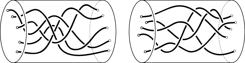
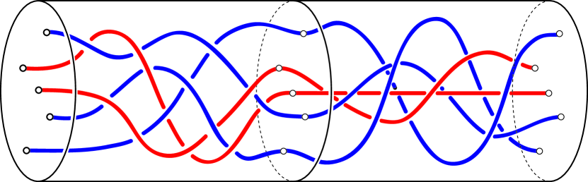
Periodic orbits of a map of ${\mathbb{D}}^{2}$ are described in terms of configuration spaces and braids. The configuration space $C^{n}({\mathbb{D}}^{2})$ is the space of all subsets of ${\mathbb{D}}^{2}$ of cardinality $n$, with the topology inherited from the product $({\mathbb{D}}^{2})^{n}$. The free loop space $\Omega^{n}$ of maps ${\mathbb{S}}^{1}\to C^{n}({\mathbb{D}}^{2})$ captures the manner in which periodic orbits ‘braid’ themselves in the Hamiltonian flow on ${\mathbb{S}}^{1}\times{\mathbb{D}}^{2}$, as in Fig. 2.1. Recall that the classical braid group ${\mathcal{B}}_{n}$ on $n$ strands is $\pi_{1}(C^{n}({\mathbb{D}}^{2}))$ (pointed homotopy classes of loops). Although elements of $\Omega^{n}$ are not themselves elements of ${\mathcal{B}}_{n}$, we abuse notation and refer to such as braids.

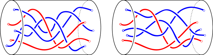
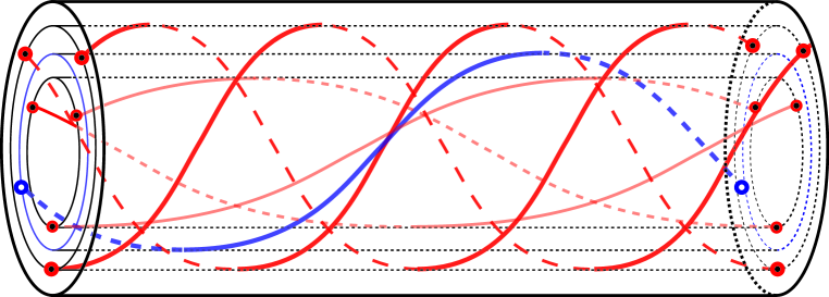
To build a forcing theory, we work with relative braids — braids split into ‘free’ and ‘skeletal’ sub-braids. Denote by $\Omega^{n,m}$ the embedded image of $\Omega^{n}\times\Omega^{m}\hookrightarrow\Omega^{n+m}$. Such a relative braid is denoted by $\textsc{x}{~{}{\rm rel}~{}}\textsc{y}$; its braid class $[\textsc{x}{~{}{\rm rel}~{}}\textsc{y}]$ is the connected component in $\Omega^{n,m}$. A relative braid class fiber $[\textsc{x}]{~{}{\rm rel}~{}}\textsc{y}$ is defined to be the subset of $\textsc{x}^{\prime}\in\Omega^{n}$ for which $\textsc{x}^{\prime}{~{}{\rm rel}~{}}\textsc{y}\in[\textsc{x}{~{}{\rm rel}~{}}\textsc{y}]$. This class represents all possible free braids which stay in the braid class, keeping the skeleton y fixed: see Fig. 2.2.

2.1.2. The variational approach

Fix a Hamiltonian $H\in{\mathscr{H}}$ and assume that $\textsc{y}\in\Omega^{n}$ is a (collection of) periodic orbit(s) of the Hamiltonian flow. We will assign a Floer homology to relative braid classes $[\textsc{x}]{~{}{\rm rel}~{}}\textsc{y}$. Define the action of $H\in{\mathscr{H}}$ via

$${\mathscr{L}}_{H}(\textsc{x})=\int_{0}^{1}\theta(\textsc{x}(t))=\int_{0}^{1}\overline{\alpha}_{0}(\textsc{x}_{t}(t))dt-\int_{0}^{1}{{\overline{H}}}(t,\textsc{x}(t))dt,$$ (2.1.2)

where $\overline{\alpha}_{0}=\sum_{k}p^{k}dq^{k}$, ${{\overline{H}}}(t,\textsc{x}(t))=\sum_{k}H(t,x^{k}(t))$; $\textsc{x}_{t}=\frac{d\textsc{x}}{dt}$; and $\theta=\overline{\alpha}_{0}-\overline{H}dt$. The set of critical points of ${\mathscr{L}}_{H}$ in $[\textsc{x}]{~{}{\rm rel}~{}}\textsc{y}$ is denoted by ${\rm Crit}_{H}([\textsc{x}]{~{}{\rm rel}~{}}\textsc{y})$.

Figure 2.2. Shown are two relative braids in the fiber $[\textsc{x}]{~{}{\rm rel}~{}}\textsc{y}$: the fixed strands y are called the skeleton.

We investigate critical points of ${\mathscr{L}}_{H}$ via nonlinear Cauchy-Riemann equations as an $L^{2}$-gradient flow of ${\mathscr{L}}_{H}$ on $[\textsc{x}]{~{}{\rm rel}~{}}\textsc{y}$. Choose a smooth $t$-dependent family of compatible almost-complex structures $J$ on $({\mathbb{D}}^{2},\omega_{0})$: each being a mapping $J:T{\mathbb{D}}^{2}\to T{\mathbb{D}}^{2}$, with $J^{2}=-{\rm Id}$, $\omega_{0}(J\cdot,J\cdot)=\omega_{0}(\cdot,\cdot)$ and $g(\cdot,\cdot)=\omega_{0}(\cdot,J\cdot)$ a metric on ${\mathbb{D}}^{2}$. We denote the set of $t$-dependent almost complex structures on ${\mathbb{D}}^{2}$ by ${\mathscr{J}}={\mathscr{J}}({\mathbb{S}}^{1}\times{\mathbb{D}}^{2})$. For functions $u:{\mathbb{R}}\times{\mathbb{R}}\to{\mathbb{D}}^{2}$ the nonlinear Cauchy-Riemann equations (CRE) are defined as

$$\bigl{(}\partial_{J,H}(u)\bigr{)}(s,t)\stackrel{{\scriptstyle\mbox{\tiny{\raisebox{0.0pt}[0.0pt][0.0pt]{def}}}}}{{=}}\frac{\partial u(s,t)}{\partial s}-J(t,u(s,t))\frac{\partial u(s,t)}{\partial t}-\nabla_{g}H(t,u(s,t)),$$ (2.1.3)

where $\nabla_{g}$ is the gradient with respect to the metric $g$. Stationary, or $s$-independent solutions $u(s,t)=x(t)$ satisfy Eq. (2.1.1) since $J\nabla_{g}H=X_{H}$. In order to find closed braids as solutions we lift the CRE to the space of closed braids: a collection $\textsc{u}(s,t)=\{u^{k}(s,t)\}$ satisfies the CRE if each component $u^{k}$ satisfies Eq. (2.1.3).

2.2. Result 1: Monotonicity

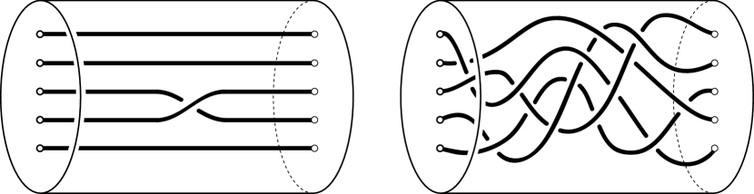
There is a crucial link between bounded solutions of CRE and algebraic-topological properties of the associated braid classes: braids decrease in word-length over time. For $\textsc{x}\in\Omega^{n}$, the associated braid can be represented as a conjugacy class in the braid group ${\mathcal{B}}_{n}$, using the standard generators $\{\sigma_{i}\}_{i=1}^{n-1}$. The length of the braid word (the sum of the exponents of the $\sigma_{i}$’s) is well-defined and is a braid invariant. Geometrically, this length is the total crossing number ${\rm Cross}(\textsc{x})$ of the braid: the algebraic sum of the number of crossings of strands in the standard planar projection (see Fig. 2.3).

Figure 2.3. The standard positive generator $\sigma_{i}$ for the braid group ${\mathcal{B}}_{n}$ sends the $i^{th}$ strand over the $(i+1)^{st}$. Pictured in ${\mathcal{B}}_{5}$ is (left) $\sigma_{2}$ and (right) the braid $\sigma_{4}^{-1}\sigma_{3}\sigma_{1}\sigma_{3}\sigma_{2}^{-1}\sigma_{1}\sigma_{2}\sigma_{3}^{-1}\sigma_{4}^{-1}\sigma_{1}\sigma_{2}\sigma_{3}\sigma_{4}^{-1}\sigma_{1}\sigma_{2}^{-1}$. This braid has length (algebraic crossing number) equal to $+3$.

To make sense of this statement, we first assemble braid classes into a completion. Denote by $\overline{\Omega}^{n}$ the space of maps ${\mathbb{S}}^{1}\to({\mathbb{D}}^{2})^{n}/S_{n}$, the configuration space of $n$ not necessarily distinct unlabeled points in ${\mathbb{D}}^{2}$. The discriminant of singular braids $\Sigma^{n}=\overline{\Omega}^{n}\backslash\Omega^{n}$ partitions $\overline{\Omega}^{n}$ into braid classes; the relative versions of these (i.e. $\textsc{x}{~{}{\rm rel}~{}}\textsc{y}$) arise when the skeleton y is fixed.

The Monotonicity Lemma 2.2 says, roughly, that the flow-lines — bounded solutions — of the CRE are transverse to the singular braids in a manner that decreases crossing number.

$\blacktriangleleft$ 2.2 Monotonicity Lemma.  Let $\textsc{u}(s)\in\overline{\Omega}^{n}$ be a local solution of the Cauchy-Riemann equations. If $\textsc{u}(s_{0},\cdot)\in\Sigma^{n}{~{}{\rm rel}~{}}\textsc{y}\stackrel{{\scriptstyle\mbox{\tiny{\raisebox{0.0pt}[0.0pt][0.0pt]{def}}}}}{{=}}\overline{\Omega}^{n}\backslash\Omega^{n}{~{}{\rm rel}~{}}\textsc{y}$, then there exists an $\epsilon_{0}>0$ such that

$${\rm Cross}(\textsc{u}(s_{0}-\epsilon,\cdot))>{\rm Cross}(\textsc{u}(s_{0}+\epsilon,\cdot))\quad\quad\forall\,0<\epsilon\leq\epsilon_{0}.$$ (2.2.1)

$\blacktriangleright$

This consequence of the maximum principle follows from the positivity of intersections of $J$-holomorphic curves in almost-complex 4-manifolds [23, 22]; other expressions of this principle arise in applications to heat equations in one space dimension, see e.g. [3, 2].

As a consequence, the local flowlines induced by the CRE are topologically transverse to the singular braids off of the (maximally degenerate) set of collapsed singular braids. This leads to an isolation property for certain relative braid classes which makes a Morse-theoretic approach viable. Denote by ${\mathscr{M}}([\textsc{x}]{~{}{\rm rel}~{}}\textsc{y})$ the set of bounded solutions $\textsc{u}(s,t)$ of the CRE contained a relative braid class $[\textsc{x}]{~{}{\rm rel}~{}}\textsc{y}$. Consider braid classes which satisfy the following topological property: for any representative $[\textsc{x}]{~{}{\rm rel}~{}}\textsc{y}$ the strands in x cannot collapse onto strands in y, or onto strands in x, nor can the strands in x collapse onto the boundary $\partial{\mathbb{D}}^{2}$. Such braid classes are called proper: see Fig. 2.4. From elliptic regularity and the Monotonicity Lemma we obtain compactness and isolation: for a proper relative braid class, the set of bounded solutions is compact and isolated in the topology of uniform convergence on compact subsets in ${\mathbb{R}}^{2}$.

Figure 2.4. Proper (left) and improper (right) relative braid classes. On the right, the free strands can collapse onto the skeleton.

$\blacktriangleleft$ 2.3 Isolation and Compactness Theorem.  Let $[\textsc{x}]{~{}{\rm rel}~{}}\textsc{y}$ be a proper braid class. Then, in the topology of uniform convergence on compact subsets in ${\mathbb{R}}^{2}$, the set of bounded solutions ${\mathscr{M}}([\textsc{x}]{~{}{\rm rel}~{}}\textsc{y})$ is compact and isolated in $[\textsc{x}]{~{}{\rm rel}~{}}\textsc{y}$. $\blacktriangleright$

The proof is a combination of Proposition 4.2 and Proposition 5.3.

2.3. Result 2: Braid Floer Homology

The above proposition is used to define a Floer homology (cf. [12]) for proper relative braid classes. Define ${\mathscr{N}}=[\textsc{x}]{~{}{\rm rel}~{}}\textsc{y}$, then by Proposition 2.4 the set of bounded solutions is in ${\mathscr{N}}$ is compact and $|\textsc{u}|<1$ for all $\textsc{u}\in{\mathscr{M}}({\mathscr{N}})$. We say that ${\mathscr{M}}({\mathscr{N}})$ is isolated. In order to define Floer homology for ${\mathscr{N}}$, the system needs to be embedded into a generic family of systems. The usual approach is to establish that (for generic choices of Hamiltonians $H\in{\mathscr{H}}$, for which $\textsc{y}\in{\rm Crit}_{H}$) the critical points of the action are non-degenerate and the sets of connecting orbits ${\mathscr{M}}_{\textsc{x}_{-},\textsc{x}_{+}}([\textsc{x}]{~{}{\rm rel}~{}}\textsc{y})$ are finite dimensional manifolds.

The Fredholm theory for CRE yields an index function $\mu$ on stationary points of the action ${\mathscr{L}}_{H}$ and $\dim{\mathscr{M}}_{\textsc{x}_{-},\textsc{x}_{+}}([\textsc{x}]{~{}{\rm rel}~{}}\textsc{y})=\mu(\textsc{x}_{-})-\mu(\textsc{x}_{+})$. Following Floer [12] we can define a chain complex $C_{k}([\textsc{x}]{~{}{\rm rel}~{}}\textsc{y})=\bigoplus{\mathbb{Z}}_{2}\langle\textsc{x}\rangle$, where the direct sum is taken over critical points of index $k$. The boundary operator $\partial_{k}:C_{k}\to C_{k-1}$ is the linear operator generated by counting orbits (modulo 2) between critical points of the correct indices. The structure of the space of bounded solutions reveals that $(C_{*},\partial_{*})$ is a chain complex. The homology of this chain complex — the braid Floer homology — is denoted ${\rm HF}_{*}([\textsc{x}]{~{}{\rm rel}~{}}\textsc{y};J,H)$. This is finite dimensional for all $k$ and nontrivial for only finitely many values of $k$. Independence of choices is our first major result. Any Hamiltonian dynamics which leaves y invariant yields the same Floer homology, ${\rm HF}_{*}([\textsc{x}]{~{}{\rm rel}~{}}\textsc{y};J,H)$ is independent of $J$ and $H$; homotopies of y within the braid class also leave the braid Floer homology invariant. To be more precise, for $\textsc{y},\textsc{y}^{\prime}\in[\textsc{y}]$, the Floer homology groups for the relative braid classes fibers $[\textsc{x}]{~{}{\rm rel}~{}}\textsc{y}$ and $[\textsc{x}^{\prime}]{~{}{\rm rel}~{}}\textsc{y}^{\prime}$ of $[\textsc{x}{~{}{\rm rel}~{}}\textsc{y}]$ are isomorphic, ${\rm HF}_{k}([\textsc{x}]{~{}{\rm rel}~{}}\textsc{y})\cong{\rm HF}_{k}([\textsc{x}^{\prime}]{~{}{\rm rel}~{}}\textsc{y}^{\prime})$. This allows us to assign the Floer homology to the entire product class $[\textsc{x}{~{}{\rm rel}~{}}\textsc{y}]$.

$\blacktriangleleft$ 2.4 Braid Floer Homology Theorem.  The braid Floer homology of a proper relative braid class,

$${\rm HB}_{*}([\textsc{x}{~{}{\rm rel}~{}}\textsc{y}])\stackrel{{\scriptstyle\mbox{\tiny{\raisebox{0.0pt}[0.0pt][0.0pt]{def}}}}}{{=}}{\rm HF}_{*}([\textsc{x}]{~{}{\rm rel}~{}}\textsc{y}),$$ (2.3.1)

is a function of the braid class $[\textsc{x}{~{}{\rm rel}~{}}\textsc{y}]$ alone, independent of choices for $J$ and $H$, and the representative skeleton y. $\blacktriangleright$

2.4. Result 3: Shifts & Twists

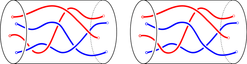
The braid Floer homology ${\rm HB}_{*}$ entwines topological braid data with dynamical information about braid-constrained Hamiltonian systems. One example of the braid-theoretic content of ${\rm HB}_{*}$ comes from an examination of twists. Recall that the braid group ${\mathcal{B}}_{n}$ has as its group operation concatenation of braids. This does not extend to a well-defined product on conjugacy classes; however, ${\mathcal{B}}_{n}$ has a nontrivial center $Z({\mathcal{B}}_{n})\cong{\mathbb{Z}}$ generated by $\Delta^{2}$, the full twist on $n$ strands. Thus, products with full twists are well-defined on conjugacy classes. These full twists have a well-defined impact on the braid Floer homology (Sec. 10). Twists shift the grading: see Fig. 2.5.

$\blacktriangleleft$ 2.5 Shift Theorem.  Let $[\textsc{x}{~{}{\rm rel}~{}}\textsc{y}]$ denote a braid class with x having $n$ strands. Then

$${\rm HB}_{*}\bigl{(}[(\textsc{x}{~{}{\rm rel}~{}}\textsc{y})\cdot\Delta^{2}]\bigr{)}\cong{\rm HB}_{*-2n}([\textsc{x}{~{}{\rm rel}~{}}\textsc{y}]).$$

$\blacktriangleright$

Figure 2.5. The addition of a full positive twist (on right) to a proper relative braid class (on left) shifts the Floer homology up by degree two.

In any Floer theory, computable examples are nontrivial. We compute examples in Sec. 11, including the following.

$\blacktriangleleft$ 2.6 Example.  Consider a skeleton y consisting of two braid components $\{\textsc{y}^{1},\textsc{y}^{2}\}$, with $\textsc{y}^{1}$ and $\textsc{y}^{2}$ defined by

$$\textsc{y}^{1}=\Bigl{\{}r_{1}e^{\tfrac{2\pi n}{m}it},\cdots,r_{1}e^{\tfrac{2\pi n}{m}i(t-m+1)}\Bigr{\}},\quad\textsc{y}^{2}=\Bigl{\{}r_{2}e^{\tfrac{2\pi n^{\prime}}{m^{\prime}}it},\cdots,r_{2}e^{\tfrac{2\pi n^{\prime}}{m^{\prime}}i(t-m^{\prime}+1)}\Bigr{\}}.$$

where $0<r_{1}<r_{2}\leq 1$, and $(n,m)$ and $(n^{\prime},m^{\prime})$ are relatively prime integer pairs with $n\not=0$, $m\geq 2$, and $m^{\prime}>0$. A free strand is given by $\textsc{x}=\{x^{1}\}$, with $x^{1}(t)=re^{2\pi\ell it}$, for $r_{1}<r<r_{2}$ and some $\ell\in{\mathbb{Z}}$, with either $n/m<\ell<n^{\prime}/m^{\prime}$ or $n/m>\ell>n^{\prime}/m^{\prime}$, depending on the ratios of $n/m$ and $n^{\prime}/m^{\prime}$. The relative braid class $[\textsc{x}{~{}{\rm rel}~{}}\textsc{y}]$ is defined via the representative $\textsc{x}{~{}{\rm rel}~{}}\textsc{y}$. The associated braid class is proper, and ${\rm HB}_{*}([\textsc{x}{~{}{\rm rel}~{}}\textsc{y}])$ is non-zero in exactly two dimensions: $2\ell$ and $2\ell\pm 1$, see Sec. 11. $\blacktriangleright$

Figure 2.6. The braid class of Example 2.4 has one free strand surrounded by a pair of skeletal braids whose rotation numbers bound from above and below.

This example agrees with a similar computation of a (finite-dimensional) Conley index of positive braid classes in [17]. Indeed, we believe that the braid Floer homology agrees with that index on positive braid classes. We anticipate using Theorem 2.4 combined with Garside’s Theorem on normal forms for braids as a means of algorithmically computing ${\rm HB}_{*}$, see e.g. Sec. 12.1.

2.5. Result 4: Forcing

Floer braid homology ${\rm HB}_{*}$ contains information about the existence of periodic points or invariant sets $A_{m}$ of area-preserving diffeomorphisms $f$. Recall that an invariant set $A_{n}=\{y^{1},\cdots,y^{n}\}$ for $f$ determines a braid class $[\textsc{y}]$ via $\textsc{y}(t)=\left(\psi_{t,H}(y^{1}),\cdots,\psi_{t,H}(y^{n})\right)$. The representation as an element $\beta(\textsc{y})$ in the braid group ${\mathcal{B}}_{n}$, given by a choice of a Hamiltoian $H$, is uniquely determined modulo full twists.

$\blacktriangleleft$ 2.7 Braid Forcing Theorem.  Let $f\in{{\rm Symp}}({\mathbb{D}}^{2},\omega_{0})$ have an invariant set $A_{m}$ representing the $m$-strand braid class $[\textsc{y}]$. Then, for any proper relative braid class $[\textsc{x}{~{}{\rm rel}~{}}\textsc{y}]$ for which ${\rm HB}_{*}([\textsc{x}{~{}{\rm rel}~{}}\textsc{y}])\not=0$, there exists an invariant set $A_{n}^{\prime}$ for $f$ such that the union $A_{m}\cup A_{n}^{\prime}$ represents the relative braid class $[\textsc{x}{~{}{\rm rel}~{}}\textsc{y}]$. $\blacktriangleright$

$\blacktriangleleft$ 2.8 Example.  Consider the braid class $[\textsc{x}{~{}{\rm rel}~{}}\textsc{y}]$ defined in Ex. 2.4. For any area-preserving diffeomorphism $f$ of the (closed) disc with invariant set represented (up to full twists) by the braid class $[\textsc{y}]$, there exist infinitely many distinct periodic points. To prove this statement we invoke the invariant ${\rm HB}_{*}$, computed in Ex. 2.4, and use Theorem 2.4. In particular, this result implies that if $f$ has a fixed point at the boundary and a periodic point of period larger than two in the interior, then $f$ has periodic points of arbitrary period, and thus infinitely many periodic points. In Sec. 11 we give more details: the main results are presented in Theorem 11.4. $\blacktriangleright$

3. Background: configuration spaces and braids

Experts who want to get to the Floer homology are encouraged to skip over the following background sections to Sec. 5.

3.1. Configuration spaces and braid classes

The configuration space $C^{n}({\mathbb{D}}^{2})$ is the space of subsets of ${\mathbb{D}}^{2}$ of cardinality $n$, with the topology inherited from the product $({\mathbb{D}}^{2})^{n}/S_{n}$, where $S_{n}$ is the permutation group. Configuration spaces lead naturally to braids [6]. For any fixed basepoint, $\pi_{1}C^{n}({\mathbb{D}}^{2})\cong{\mathcal{B}}_{n}$, Artin’s braid group on $n$ strands. For our purposes (finding periodic orbits of Hamiltonian maps of the disc), the basepoint is unnatural, and we work with free loop spaces.

The loop space $\Omega^{n}$ is the space of continuous mappings $\textsc{x}:{\mathbb{R}}/{\mathbb{Z}}\to C^{n}({\mathbb{D}}^{2})$ under the standard (strong) metric topology induced by $C^{0}({\mathbb{R}}/{\mathbb{Z}};{\mathbb{D}}^{2})$. We abuse notation to indicate points in $C^{n}({\mathbb{D}}^{2})$ and loops in $\Omega^{n}$ by the same symbol x, often referred to as a braid. In some contexts we denote loops by $\textsc{x}(t)$ and consider them as a union of disjoint ‘strands’ $x^{k}(t)$. Two loops $\textsc{x}(t)$ and $\tilde{\textsc{x}}(t)$ are close in the topology of $\Omega^{n}$ if and only if for some permutation $\theta\in S_{n}$ the strands $x^{\theta(k)}$ and $\tilde{x}^{k}$ are $C^{0}$-close for all $k$ and $\tilde{\sigma}=\theta^{-1}\sigma\theta$.

The braid class of x is the connected component $[\textsc{x}]\in\pi_{0}(\Omega^{n})$. These braid classes can be completed to $\overline{\Omega}^{n}$, the $C^{0}$-closure of $\Omega^{n}$ in $({\mathbb{D}}^{2})^{n}/S_{n}$. The discriminant $\Sigma^{n}=\overline{\Omega}^{n}\backslash\Omega^{n}$ defines the singular braids. A special subset of singular braids are those that can be regarded as in $\overline{\Omega}^{n^{\prime}}$ with $n^{\prime}<n$. Such collapsed braids are denoted by $\Sigma_{-}^{n}\subset\Sigma^{n}$.

Given a fixed skeleton braid $\textsc{y}\in\Omega^{m}$, we define the relative braids as follows. There is a natural inclusion $\iota_{\textsc{y}}:\Omega^{n}\hookrightarrow\overline{\Omega}^{n+m}$ taking x to the union of x and y — a potentially singular braid. Braids rel y are partitioned by the singular relative braids $\Sigma{~{}{\rm rel}~{}}\textsc{y}=\iota_{\textsc{y}}^{-1}(\Sigma^{n+m})$ into connected components. These connected components in $\Omega^{n,m}$ are the relative braid classes $[\textsc{x}{~{}{\rm rel}~{}}\textsc{y}]$; in this class, both the strands of x and y are permitted to deform (though without intersecting themselves or each other). The relative braid class $[\textsc{x}]{~{}{\rm rel}~{}}\textsc{y}$ is defined as the fiber $\iota_{\textsc{y}}^{-1}(\Omega^{n+m})\cap[\textsc{x}]$; in this fiber, strands of x may deform, but not strands of y.

3.2. The Hamiltonian action

For $H\in{\mathscr{H}}$ the Hamiltonian 1-form on ${\mathbb{S}}^{1}\times{\mathbb{D}}^{2}$ is defined by $\theta=pdq-Hdt$. For a loop $\textsc{x}\in\Omega^{1}$ one defines the action functional

$${\mathscr{L}}_{H}(x)=\int_{0}^{1}\theta(x(t))=\int_{0}^{1}\alpha_{0}(x_{t}(t))dt-\int_{0}^{1}H(t,x(t))dt,$$ (3.2.1)

where $\alpha_{0}=pdq$ and $x_{t}=\frac{dx}{dt}$. The first variation with respect to variations $\xi\in C^{1}$ defines an exact 1-form $d{\mathscr{L}}_{H}$:

$$d{\mathscr{L}}_{H}(x)\xi = -\int_{0}^{1}\omega_{0}\bigl{(}x_{t}(t),\xi(t)\bigr{)}dt-\int_{0}^{1}dH(t,x(t))\xi(t)dt$$

$$= -\int_{0}^{1}\omega_{0}\Bigl{(}x_{t}(t)-X_{t,H}(t,x(t)),\xi(t)\Bigr{)}dt,$$

which gives the variational principle for Eq.  (2.1.1). For closed $n$-braids we can extend the Hamiltonian action to $\overline{\Omega}^{n}$. Given any $\textsc{x}\in\overline{\Omega}^{n}$ define its action by ${\mathscr{L}}_{H}(\textsc{x})=\sum_{k=1}^{n}{\mathscr{L}}_{H}(x^{k})$. We may regard ${\mathscr{L}}_{H}(\textsc{x})$ as the action for a Hamiltonian system on $({\mathbb{D}}^{2})^{n}$, with $\overline{\omega}_{0}=\omega_{0}\times\cdots\times\omega_{0}$, and $\overline{H}(t,\textsc{x})=\sum_{k}H(t,x^{k})$, i.e. an uncoupled system with coupled boundary conditions $x^{k}(t+1)=x^{\sigma(k)}(t)$ for all $t$ and all $k=1,\cdots,n$, where $\sigma\in S_{n}$ is a permutation. We abuse notation by denoting the action for the product system by ${\mathscr{L}}_{H}(\textsc{x})$ and the action is well-defined for all $\textsc{x}\in\overline{\Omega}^{n}\cap C^{1}$. The stationary, or critical closed braids, including singular braids, are denoted by ${\rm Crit}_{H}(\overline{\Omega}^{n})=\bigl{\{}\textsc{x}\in\overline{\Omega}^{n}\cap C^{1}~{}|~{}d{\mathscr{L}}_{H}(\textsc{x})=0\bigr{\}}.$ By the boundary conditions given above, the first variation of the action yields that the individual strands satisfy Eq. (2.1.1). For the critical points of ${\mathscr{L}}_{H}$ on $\overline{\Omega}^{n}$ the following compactness property holds.

$\blacktriangleleft$ 3.1 Lemma.  The set ${\rm Crit}_{H}(\overline{\Omega}^{n})$ is compact in $\overline{\Omega}^{n}$. As a matter of fact ${\rm Crit}_{H}(\overline{\Omega}^{n})$ is compact in the $C^{r}$-topology for any $r\geq 1$. $\blacktriangleright$

Proof.    From Eq.  (2.1.1) we derive that $|x_{t}^{k}|=|\nabla H(t,x^{k})|\leq C$, by the assumptions on $H$. Since $|x^{k}|\leq 1$, for all $k$, we obtain the a priori estimate $\|\textsc{x}\|_{W^{1,\infty}}\leq C,$ which holds for all $\textsc{x}\in{\rm Crit}_{H}(\overline{\Omega}^{n})$. Via compact embeddings (Arzela-Ascoli) we have that a sequence $\textsc{x}_{n}\in{\rm Crit}_{H}$ converges in $C^{0}$, along a subsequence, to a limit $\textsc{x}\in\overline{\Omega}^{n}$. Using the equation we obtain the convergence in $C^{1}$ and x satisfies the equation with the boundary conditions given above. Therefore $\textsc{x}\in{\rm Crit}_{H}(\overline{\Omega}^{n})$, thereby establishing the compactness of ${\rm Crit}_{H}(\overline{\Omega}^{n})$ in $\overline{\Omega}^{n}$. The $C^{r}$-convergence is achieved by differentiating Eq. (2.1.1) repeatedly. This concludes the compactness of ${\rm Crit}_{H}(\overline{\Omega}^{n})$ in $C^{r}$. $\Box$

$\blacktriangleleft$ 3.2 Remark.  The critical braids in ${\rm Crit}_{H}(\overline{\Omega}^{n})$ have one additional property that plays an important role. For the strands $x^{k}$ of $\textsc{x}\in{\rm Crit}_{H}(\overline{\Omega}^{n})$ it holds that either $|x^{k}(t)|=1$, for all $t$, or $|x^{k}(t)|<1$, for all $t$. This is a consequence of the uniqueness of solutions for the initial value problem for (2.1.1). We say that a braid x in supported in ${\rm int}({\mathbb{D}}^{2})$ if $|x^{k}(t)|<1,$ for all $t$ and for all $k$. $\blacktriangleright$

In the same spirit, we can define the subset of stationary braids restricted to a braid class $[\textsc{x}]$, notation ${\rm Crit}_{H}([\textsc{x}])$, or in the case of a relative braid class ${\rm Crit}_{H}([\textsc{x}]{~{}{\rm rel}~{}}\textsc{y})$.

4. Background: Cauchy-Riemann equations

4.1. Almost complex structures

The standard almost complex matrix $J_{0}$ is defined by the relation $\langle\cdot,\cdot\rangle=\omega_{0}(\cdot,J_{0}\cdot)$, where $\langle\cdot,\cdot\rangle$ is the standard inner product defined by $dp\otimes dp+dq\otimes dq$. Therefore, $J_{0}$ defines an almost complex structure on ${\mathbb{D}}^{2}$ which corresponds to complex multiplictation with $i$ in ${\mathbb{C}}$. In general an almost complex structure on ${\mathbb{D}}^{2}$ is a mapping $J:T{\mathbb{D}}^{2}\to T{\mathbb{D}}^{2}$, with the property that $J^{2}=-{\rm id}$. An almost complex structure is compatible with $\omega_{0}$ if $\omega_{0}(\cdot,J\cdot)$ defines a metric on ${\mathbb{D}}^{2}$ and $g=\omega_{0}(\cdot,J\cdot)$ is $J$-invariant. The space of $t$-families of almost complex structures is denoted by ${\mathscr{J}}={\mathscr{J}}({\mathbb{S}}^{1}\times{\mathbb{D}}^{2})$.

In terms of the standard inner product $\langle\cdot,\cdot\rangle$ the metric $g$ is given by $g(\xi,\eta)=\langle-J_{0}J\xi,\eta\rangle$, where $-J_{0}J$ is a positive definite symmetric matrix function. With respect to the metric $g$ it holds that $J\nabla_{g}H=X_{H}$.

4.2. Compactness

In order to study 1-periodic solutions of Eq.  (2.1.1) the variational method due to Floer and Gromov explores the perturbed nonlinear Cauchy-Riemann equations (2.1.3) which can be rewritten as

$${\partial_{J,H}}(u)=u_{s}-J(t,u)\bigl{[}u_{t}-X_{H}(t,u)\bigr{]}=0,$$

for functions $u:{\mathbb{R}}\times{\mathbb{R}}\to{\mathbb{D}}^{2}$ (short hand notation). In the case of 1-periodic solutions we invoke the boundary conditions $u(s,t+1)=u(s,t)$.

In order to find closed braids as critical points of ${\mathscr{L}}_{H}$ on $\overline{\Omega}^{n}$ we invoke the CRE for $u^{k}$ in $\textsc{u}=\{u^{k}\}$. A collection of $C^{1}$-functions $\textsc{u}(s,t)=\{u^{k}(s,t)\}$ is said to satisfy the CRE if its components $u^{k}$ satisfy Eq. (2.1.3) for all $k$ and the periodicity condition

$$\{u^{1}(s,t+1),\dots,u^{n}(s,t+1)\}=\{u^{1}(s,t),\dots,u^{n}(s,t)\}.$$ (4.2.1)

for all $s,t$. We use the almost complex structure $\overline{J}$ defined via $\overline{g}(\cdot,\cdot)=\overline{\omega}_{0}(\cdot,\overline{J}\cdot)$, $\overline{\omega}_{0}=\omega_{0}\times\cdots\times\omega_{0}$, and $\overline{g}(\cdot,\cdot)=\overline{\omega}_{0}(\cdot,\overline{J}\cdot)$, with $\overline{H}(t,\textsc{x})=\sum_{k}H(t,x^{k})$ as per Sect. 2.1.2. The equations become

$$\partial_{\overline{J},\overline{H}}(\textsc{u})=\textsc{u}_{s}-\overline{J}(t,\textsc{u})\bigl{[}\textsc{u}_{t}-X_{{{\overline{H}}}}(t,\textsc{u})\bigr{]}=0,$$ (4.2.2)

where $X_{{{\overline{H}}}}$ is defined via the relation $\iota_{X_{t,{{\overline{H}}}}}\overline{\omega}_{0}=-d{{\overline{H}}}$ and the periodicity condition in (4.2.1). This requirement is fulfilled precisely by braids $\textsc{u}(s,\cdot)\in\overline{\Omega}^{n}$ for all $s$. We therefore define the space of bounded solutions in the space of $n$-braids by:

$${\mathscr{M}}^{J,H}={\mathscr{M}}^{J,H}(\overline{\Omega}^{n})=\bigl{\{}\textsc{u}=\{u^{k}\}\in C^{1}\bigl{(}{\mathbb{R}}\times{\mathbb{R}}/{\mathbb{Z}};C^{n}({\mathbb{D}}^{2})\bigr{)}~{}|~{}\partial_{J,H}(u^{k})=0,~{}~{}\forall k\bigr{\}}$$

Note that solutions in ${\mathscr{M}}^{J,H}$ extend to $C^{1}$-functions $u^{k}:{\mathbb{R}}\times{\mathbb{R}}\to{\mathbb{D}}^{2}$ by periodic extension in $t$. If there is no ambiguity about the dependence on $J$ and $H$ we abbreviate notation by writing ${\mathscr{M}}$ instead of ${\mathscr{M}}^{J,H}$.

The following statement is Floer’s compactness theorem adjusted to the present situation.

$\blacktriangleleft$ 4.1 Proposition.  The space ${\mathscr{M}}^{J,H}$ is compact in the topology of uniform convergence on compact sets in $(s,t)\in{\mathbb{R}}^{2}$, with derivatives up to any order. The action ${\mathscr{L}}_{H}$ is uniformly bounded along trajectories $\textsc{u}\in{\mathscr{M}}^{J,H}$, and

$$\lim_{s\to\pm\infty}|{\mathscr{L}}_{H}(\textsc{u}(s,\cdot))|=|c_{\pm}(\textsc{u})|\leq C(J,H),$$

$$\int_{\mathbb{R}}\int_{0}^{1}|\textsc{u}_{s}|_{g}^{2}dtds=\sum_{k=1}^{n}\int_{\mathbb{R}}\int_{0}^{1}|u_{s}^{k}|_{g}^{2}dtds\leq C^{\prime}(J,H),$$

for all $\textsc{u}\in{\mathscr{M}}^{J,H}$ and some constants $c_{\pm}(\textsc{u})$. The constants $C,\,C^{\prime}$ depend only on $J\in{\mathscr{J}}$ and $H\in{\mathscr{H}}$. $\blacktriangleright$

Proof.    Define the operators

$$\partial_{J}=\frac{\partial}{\partial s}-J\frac{\partial}{\partial t},\quad\bar{\partial}_{J}=\frac{\partial}{\partial s}+J\frac{\partial}{\partial t}.$$

Eq.  (2.1.3) can now be written as $\partial_{J}u^{k}=\nabla_{g}H(t,u^{k})\stackrel{{\scriptstyle\mbox{\tiny{\raisebox{0.0pt}[0.0pt][0.0pt]{def}}}}}{{=}}f^{k}(s,t)$ for all $k$. By the hypotheses on $H$ and the fact that $|u^{k}|\leq 1$ for all $k$ we have that $f^{k}(s,t)\in L^{\infty}({\mathbb{R}}^{2})$. The latter follows from the fact that the solutions $u^{k}$ can be regarded as functions on ${\mathbb{R}}^{2}$ via periodic extension in $t$. Using these crucial a priori estimates, the remainder follows as in Floer’s compactness proof: see [32, 33]. In brief, the $L^{\infty}$-estimates yield $C^{1,\lambda}$-estimates, which then give the desired compactness. By the smoothness of $J$ and $H$ such estimates can be found in any $C^{r,\lambda}$.

Due to the a priori bound in $C^{1,\lambda}$ it holds that $|{\mathscr{L}}_{H}(\textsc{u}(s,\cdot))|\leq C(J,H)$ and since

$$\frac{d}{ds}{\mathscr{L}}_{H}(\textsc{u}(s,\cdot))=-\int_{0}^{1}|\textsc{u}_{s}|_{g}^{2}dt\leq 0,$$

it follows that the limits $\lim_{s\to\pm\infty}{\mathscr{L}}_{H}(\textsc{u}(s,\cdot))=c_{\pm}$ exist and are a priori bounded by the same constant $C(J,H)$. Finally, for any $T_{1},T_{2}>0$,

$$\int_{-T_{1}}^{T_{2}}\int_{0}^{1}|\textsc{u}_{s}|_{g}^{2}dtds=\sum_{k=1}^{n}\int_{-T_{1}}^{T_{2}}\int_{0}^{1}|u_{s}^{k}|_{g}^{2}dtds={\mathscr{L}}_{H}(\textsc{u}(T_{2},\cdot))-{\mathscr{L}}_{H}(\textsc{u}(-T_{1},\cdot)).$$

By the uniform boundedness of the action along all orbits $\textsc{u}\in{\mathscr{M}}_{J,H}$ we obtain the estimate $\int_{\mathbb{R}}\int_{0}^{1}|\textsc{u}_{s}|_{g}^{2}dtds\leq 2C(J,H),$ which completes our proof. $\Box$

$\blacktriangleleft$ 4.2 Remark.  In the above proof we only use $C^{2}$-regularity of the Hamiltonian $H$ in order to obtain compactness in $C^{1}$. Since we assume Hamiltonians to be $C^{\infty}$-smooth we can improve the compactness result to hold up to derivatives of any order. $\blacktriangleright$

4.3. Additional compactness

Consider the non-autonomous Cauchy-Riemann equations:

$$u_{s}-J(s,t,u)u_{t}-\nabla_{g_{s}}H(s,t,u)=0,$$ (4.3.1)

where $s\mapsto J(s,\cdot)$ is a smooth path in ${\mathscr{J}}$ and $s\mapsto H(s,\cdot,\cdot)$ is a smooth path in ${\mathscr{H}}$. Both paths are assumed to have the property that the limits as $s\to\pm\infty$ exists. The path of metrics $s\mapsto g_{s}$ is defined via the relation $g_{s}(\cdot,\cdot)=\omega_{0}(\cdot,J(s,\cdot)\cdot)$. Assume that $|H_{s}|\leq\kappa(s)\to 0$ as $s\to\pm\infty$ uniformly in $(t,x)\in{\mathbb{R}}/{\mathbb{Z}}\times{\mathbb{D}}^{2}$, with $\kappa\in L^{1}({\mathbb{R}})$. For the equation $\partial_{J}v=f(s,t)$, the analogue of Proposition 4.2 holds via the $L^{\infty}$-estimates on the right hand side, see [32, 33]. We sketch the main idea.

Define $s\mapsto{\mathscr{L}}_{H}(s,x)$ as the action path with Hamiltonian path $s\mapsto H(s,\cdot,\cdot)$. The first variation with respect to $s$ can be computed as before:

$$\frac{d}{ds}{\mathscr{L}}_{H}(s,\textsc{u}(s,\cdot)) = \frac{\partial{\mathscr{L}}_{H}}{\partial s}+\sum_{k=1}^{n}\int_{0}^{1}\omega_{0}\bigl{(}u_{t}^{k}-X_{H}(t,u^{k}),u^{k}_{s}\bigr{)}dt$$

$$= \frac{\partial{\mathscr{L}}_{H}}{\partial s}-\sum_{k=1}^{n}\int_{0}^{1}|u_{t}^{k}-X_{H}(t,u^{k})|^{2}_{g_{s}}dt$$

$$= \frac{\partial{\mathscr{L}}_{H}}{\partial s}-\int_{0}^{1}|\textsc{u}_{s}|^{2}_{g_{s}}dt.$$

The partial derivative with respect to $s$ is given by

$$\frac{\partial{\mathscr{L}}_{H}}{\partial s}=\sum_{k=1}^{n}\int_{0}^{1}\frac{\partial H}{\partial s}\left(s,t,u^{k}(s,t)\right)dt,$$

and $\left|\frac{\partial{\mathscr{L}}_{H}}{\partial s}\right|\leq C\kappa(s)\to 0$ as $s\to\pm\infty$. For a non-stationary solution u it holds that $\int_{0}^{1}|\textsc{u}_{s}|^{2}_{g_{s}}dt>0$, and thus for $|s|$ sufficiently large $\frac{d}{ds}{\mathscr{L}}_{H}(s,\textsc{u}(s,\cdot))-\frac{\partial}{\partial s}{\mathscr{L}}_{H}<0$, proving that the limits $\lim_{s\to\pm\infty}{\mathscr{L}}_{H}(s,\textsc{u}(s,\cdot))=c_{\pm}$ exist. Since $\kappa\in L^{1}({\mathbb{R}})$ we also obtain the integral $\int_{\mathbb{R}}\int_{0}^{1}|\textsc{u}_{s}|^{2}_{g_{s}}dtds\leq C(J,H)$. This non-autonomous CRE will be used to establish continuation for Floer homology.

5. Crossing numbers, a priori estimates and isolation

5.1. The crossing number

We begin with an important property of the (linear) Cauchy-Riemann equations in dimension two. We consider Eq. (2.1.3), or more generally Equation (4.3.1), and local solutions of the form $u:G\subset{\mathbb{R}}^{2}\to{\mathbb{R}}^{2}$, where $G=[\sigma,\sigma^{\prime}]\times[\tau,\tau^{\prime}]$. For two local solutions $u,u^{\prime}:G\to{\mathbb{R}}^{2}$ of (2.1.3) assume that

$$u(s,t)\not=u^{\prime}(s,t),~{}~{}~{}{\rm for~{}all}~{}~{}(s,t)\in\partial G.$$

Intersections of $u$ and $u^{\prime}$, where $u(s_{0},t_{0})=u^{\prime}(s_{0},t_{0})$ for some $(s_{0},t_{0})\in G$, have constrained evolutions. Consider the difference function $w(s,t)=u(s,t)-u^{\prime}(s,t)$. By the assumptions on $u$ and $u^{\prime}$ we have that $w|_{\partial G}\not=0$, and intersections are given by $w(s_{0},t_{0})=0$. The following lemma is a special feature of CRE in dimension two and is a manifestation of the well-known positivity of intersection of $J$-holomorphic curves in almost complex 4-manifolds [23, 22].

$\blacktriangleleft$ 5.1 Lemma.  Let $u,u^{\prime}$ and $G$ be as defined above. Assume that $w(s_{0},t_{0})=0$ for some $(s_{0},t_{0})\in G$. Then $(s_{0},t_{0})$ is an isolated zero and $\deg(w,G,0)<0$. $\blacktriangleright$

Proof.    Taylor expand: $\nabla_{g}H(t,u^{\prime})=\nabla_{g}H(t,u)+R_{1}(t,u,u^{\prime}-u)(u^{\prime}-u)$, where $R_{1}$ is continuous. Substitution yields

$$w_{s}-J(s)w_{t}-A(s,t)w=0,\quad w(s_{0},t_{0})=0,$$

where $A(s,t)=R_{1}(t,u,-w)$ is continuous on $G$. Define complex coordinates $z=s-s_{0}+i(t-t_{0})$. Then by [20, Appendix A.6], there exists a $\delta<0$, sufficiently small, a disc $D_{\delta}=\{z~{}|~{}|z|\leq\delta\}$, a holomorphic map $h:D_{\delta}\to{\mathbb{C}}$, and a continuous mapping $\Phi:D_{\delta}\to{\rm GL}_{{\mathbb{R}}}({\mathbb{C}})$ such that

$$\det~{}\Phi(z)>0,\qquad J(z)\Phi(z)=\Phi(z)i,\qquad w(z)=\Phi(z)\bar{h}(z),$$

for all $z\in D_{\delta}$. Clearly, $\Phi$ can be represented by a real $2\times 2$ matrix function of invertible matrices.

Since $w=\Phi\bar{h}$, it holds that the condition $w(z_{0})=0$ implies that $\bar{h}(z_{0})=h(z_{0})=0$. The analyticity of $h$ then implies that either $z_{0}$ is an isolated zero in $D_{\delta}$, or $h\equiv 0$ on $D_{\delta}$. If the latter holds, then also $w\equiv 0$ on $D_{\delta}$. If we repeat the above arguments we conclude that $w\equiv 0$ on $G$ (cf. analytic continuation), in contradiction with the boundary conditions. Therefore, all zeroes of $w$ in $G$ are isolated, and there are finitely many zeroes $z_{i}\in{\rm int}(G)$.

For the degree we have that, since $\det\Phi(z)>0$,

$$\deg(w,G,0)=\sum_{i=1}^{m}\deg(w,B_{\epsilon_{i}}(z_{i}),0)=\sum_{i=1}^{m}\deg(\bar{h},B_{\epsilon_{i}}(z_{i}),0)=-\sum_{i=1}^{m}\deg(h,B_{\epsilon_{i}}(z_{i}),0),$$

and for an analytic function with an isolated zero $z_{i}$ it holds that $\deg(h,B_{\epsilon_{i}}(z_{i}),0)=n_{i}\geq 1$; thus $\deg(w,G,0)<0$. $\Box$

For a curve $\Gamma:I\to{\mathbb{R}}^{2}\setminus\{(0,0)\}$, with $I$ a bounded interval, one can define the winding number about the origin by

$$W(\Gamma,0)\stackrel{{\scriptstyle\mbox{\tiny{\raisebox{0.0pt}[0.0pt][0.0pt]{def}}}}}{{=}}\frac{1}{2\pi}\int_{I}\Gamma^{*}\alpha=\frac{1}{2\pi}\int_{\Gamma}\alpha,$$

for $\alpha=(-qdp+pdq)/(p^{2}+q^{2})$. In particular, for curves $w(s,\cdot):[\tau,\tau^{\prime}]\to{\mathbb{R}}^{2}\setminus\{(0,0)\}$ and for $s=\sigma,\sigma^{\prime}$ the (local) winding number is

$$W(w(s,\cdot),0)\stackrel{{\scriptstyle\mbox{\tiny{\raisebox{0.0pt}[0.0pt][0.0pt]{def}}}}}{{=}}\frac{1}{2\pi}\int_{[\tau,\tau^{\prime}]}w^{*}\alpha=\frac{1}{2\pi}\int_{w}\alpha.$$

We denote these winding numbers by $W_{\sigma}^{[\tau,\tau^{\prime}]}(w)$ and $W_{\sigma^{\prime}}^{[\tau,\tau^{\prime}]}(w)$ respectively. In the case that $[\tau,\tau^{\prime}]=[0,1]$ we simply write $W_{\sigma}(w)\stackrel{{\scriptstyle\mbox{\tiny{\raisebox{0.0pt}[0.0pt][0.0pt]{def}}}}}{{=}}W_{\sigma}^{[0,1]}(w)$. Similarly, we have winding numbers for the curves $w(\cdot,t):[\sigma,\sigma^{\prime}]\to{\mathbb{R}}^{2}\setminus\{(0,0)\}$ and for $t=\tau,\tau^{\prime}$, which we denote by $W_{\tau}^{[\sigma,\sigma^{\prime}]}(w)$ and $W_{\tau^{\prime}}^{[\sigma,\sigma^{\prime}]}(w)$ respectively. These local winding numbers are related to the degree of the map $w:G\to{\mathbb{R}}^{2}$.

$\blacktriangleleft$ 5.2 Lemma.  Let $u,u^{\prime}:G\to{\mathbb{R}}^{2}$ be local solutions of Equation (2.1.3), with $w|_{\partial G}\not=0$. Then

$$\Bigl{[}W_{\sigma^{\prime}}^{[\tau,\tau^{\prime}]}(w)-W_{\sigma}^{[\tau,\tau^{\prime}]}(w)\Bigr{]}-\Bigl{[}W_{\tau^{\prime}}^{[\sigma,\sigma^{\prime}]}(w)-W_{\tau}^{[\sigma,\sigma^{\prime}]}(w)\Bigr{]}=\deg(w,G,0).$$ (5.1.1)

In particular, for each zero $(s_{0},t_{0})\in{\rm int}(G)$, there exists an $\epsilon_{0}>0$ such that

$$W_{s_{0}+\epsilon}^{[\tau,\tau^{\prime}]}(w)-W_{s_{0}-\epsilon}^{[\tau,\tau^{\prime}]}(w)<W_{\tau^{\prime}}^{[s_{0}-\epsilon,s_{0}+\epsilon]}(w)-W_{\tau}^{[s_{0}-\epsilon,s_{0}+\epsilon]}(w),$$

for all $0<\epsilon\leq\epsilon_{0}$. $\blacktriangleright$

Proof.    We abuse notation by regarding $w$ as a map from the complex plane to itself. Let the contour $\gamma=\partial G$ be positively oriented (counterclockwise in the $(s,t)$ plane). The winding number of the contour $w(\gamma)$ about $0\in{\mathbb{C}}$ in complex notation is given by

$$W(w(\gamma),0)=\frac{1}{2\pi i}\oint_{w(\gamma)}\frac{dz}{z}=\deg(w,G,0),$$

which is equal to the degree of $w:G\to{\mathbb{R}}^{2}$ with respect to the value $0$. Using the special form of the contour $\gamma$ we can write out the the Cauchy integral using the 1-form $\alpha$:

$$\frac{1}{2\pi i}\oint_{w(\gamma)}\frac{dz}{z} = \frac{1}{2\pi}\int_{w(\sigma^{\prime},\cdot)}\alpha-\frac{1}{2\pi}\int_{w(\cdot,\tau^{\prime})}\alpha-\frac{1}{2\pi}\int_{w(\sigma,\cdot)}\alpha+\frac{1}{2\pi}\int_{w(\cdot,\tau)}\alpha$$

$$= \Bigl{[}W_{\sigma^{\prime}}^{[\tau,\tau^{\prime}]}(w)-W_{\sigma}^{[\tau,\tau^{\prime}]}(w)\Bigr{]}-\Bigl{[}W_{\tau^{\prime}}^{[\sigma,\sigma^{\prime}]}(w)-W_{\tau}^{[\sigma,\sigma^{\prime}]}(w)\Bigr{]},$$

which proves the first statement.

Lemma 5.1 states that all zeroes of $w$ are isolated and have negative degree. Therefore, there exists an $\epsilon_{0}>0$ such that $G_{\epsilon}=[s_{0}-\epsilon,s_{0}+\epsilon]\times[\tau,\tau^{\prime}]$ contains no zeroes on the boundary, for all $0<\epsilon\leq\epsilon_{0}$, from which the second statement follows. $\Box$

On the level of comparing two local solutions of Equation (2.1.3), the winding number behaves like a discrete Lyapunov function with respect to the time variable $s$. This can be further formalized for solutions of the CRE on $\overline{\Omega}^{n}$. For a closed braid $\textsc{x}\in\Omega^{n}$, one defines the total crossing number

$${\rm Cross}(\textsc{x})\stackrel{{\scriptstyle\mbox{\tiny{\raisebox{0.0pt}[0.0pt][0.0pt]{def}}}}}{{=}}\sum_{k,k^{\prime}}W\bigl{(}x^{k}-x^{k^{\prime}},0\bigr{)}=2\sum_{\{k,k^{\prime}\}\atop k\neq k^{\prime}}W\bigl{(}x^{k}-x^{k^{\prime}},0\bigr{)},$$ (5.1.2)

where the second sum is over all unordered pairs $\{k,k^{\prime}\}$, using the fact that the winding number is invariant under the inversion $(p,q)\to(-p,-q)$. The number ${\rm Cross}(\textsc{x})$ is equal to the total linking/self-linking number of all components in a closed braid x. The local winding number as introduced above is not necessarily an integer. However, for closed curves the winding number is integer valued. It is clear that the number ${\rm Cross}(\textsc{x})$ as defined above is also an integer, one interpretation of which is via the associated braid diagrams as the algebraic crossing number:

$\blacktriangleleft$ 5.3 Lemma.  The number ${\rm Cross}(\textsc{x})$ is an integer, and

$${\rm Cross}(\textsc{x}) = \#\{\hbox{positive crossings}\}-\#\{\hbox{negative crossings}\}.$$

This is a braid class invariant; i.e., ${\rm Cross}(\textsc{x})={\rm Cross}(\textsc{x}^{\prime})$ for all $\textsc{x},\textsc{x}^{\prime}\in[\textsc{x}]$. $\blacktriangleright$

This result is standard: we include a self-contained proof.

Proof.    The expression for ${\rm Cross}(\textsc{x})$ is twice the sum of $\tfrac{n!}{2!(n-2)!}$ local winding numbers. On the unordered pairs $\{k,k^{\prime}\}$ there exists the following equivalence relation. Two pairs $\{k,k^{\prime}\}$ and $\{h,h^{\prime}\}$ are equivalent if for some integer $d\geq 0$, $\{x^{k}(d),x^{k^{\prime}}(d)\}=\{x^{h}(0),x^{h^{\prime}}(0)\}$ as unordered pairs. The equivalence classes of unordered pairs $\{k,k^{\prime}\}$ are denoted by $\pi_{j}$ and the number of elements in $\pi_{j}$ is denoted by $|\pi_{j}|$. For each class $\pi_{j}$ define $w_{\pi_{j}}=x^{k}-x^{k^{\prime}}$, for some representative $\{k,k^{\prime}\}\in\pi_{j}$. For $t\in[0,2|\pi_{j}|]$, the functions $w_{\pi_{j}}(t)$ represent closed loops in ${\mathbb{R}}^{2}$ regardless of the choice of the representative $\{k,k^{\prime}\}\in\pi_{j}$. Namely, note that $\{x^{k}(|\pi_{j}|),x^{k^{\prime}}(|\pi_{j}|)\}=\{x^{k}(0),x^{k^{\prime}}(0)\}$ as unordered pairs, which imlies that

$$x^{k}(|\pi_{j}|)=x^{k}(0)\qquad\text{or}\qquad x^{k}(|\pi_{j}|)=x^{k^{\prime}}(0).$$ (5.1.3)

For the crossing number we have

$${\rm Cross}(\textsc{x})=2\sum_{j}\Bigl{(}\sum_{\{k,k^{\prime}\}\in\pi_{j}}W\bigl{(}x^{k}-x^{k^{\prime}},0\bigr{)}\Bigr{)}=2\sum_{j}W^{[0,|\pi_{j}|]}(w_{\pi_{j}},0)=\sum_{j}W^{[0,|2\pi_{j}|]}(w_{\pi_{j}},0),$$ (5.1.4)

where the (outer) sum is over all equivalence classes $\pi_{j}$. For the final equality we have used (5.1.3) and the invariance of the winding number under the inversion $w\to-w$. Since the latter winding numbers are winding numbers for closed loops about $0$ (linking numbers), they are all integers, and thus ${\rm Cross}(\textsc{x})$ is an integer.

As for the expression in terms of positive and negative crossings we argue as follows. By inspection, $W\bigl{(}x^{k}-x^{k^{\prime}},0\bigr{)}$ equals all positive minus negative crossings between the two strands. The invariance of ${\rm Cross}(\textsc{x})$ with respect to $[\textsc{x}]$ follows from the homotopy invariance of the winding number. $\Box$

Using the representation of the crossing number for a braid in terms of winding numbers, we can prove a Lyapunov property. Note that elements u of ${\mathscr{M}}$ are not necessarily in $\Omega^{n}$ for all $s$. Therefore ${\rm Cross}(\textsc{u}(s,\cdot))$ is only well-defined whenever $\textsc{u}(s,\cdot)\in\Omega^{n}$.

Combining these results leads to the crucial step in setting up a Floer theory for braid classes.

$\blacktriangleleft$ 5.4 Lemma.  [Monotonicity Lemma] For $\textsc{u}\in{\mathscr{M}}$, ${\rm Cross}(\textsc{u}(s,\cdot))$ is (when well-defined) non-increasing in $s$. To be more precise, if $u^{k}(s_{0},t_{0})=u^{k^{\prime}}(s_{0},t_{0})$ for some $(s_{0},t_{0})\in{\mathbb{R}}\times{\mathbb{R}}/{\mathbb{Z}}$, and $k\not=k^{\prime}$, then either there exists an $\epsilon_{0}>0$ such that

$${\rm Cross}(\textsc{u}(s_{0}-\epsilon,\cdot))>{\rm Cross}(\textsc{u}(s_{0}+\epsilon,\cdot)),$$

for all $0<\epsilon\leq\epsilon_{0}$, or $u^{k}\equiv u^{k^{\prime}}$. $\blacktriangleright$

Proof.    Given $\textsc{u}=\{u^{k}\}\in{\mathscr{M}}$, ${\rm Cross}(\textsc{u}(s,\cdot))$ is well-defined for all $s\in{\mathbb{R}}$ for which $\textsc{u}(s,\cdot)\in\Omega^{n}$. As in the proof of Lemma 5.1 we define $w_{\pi_{j}}(s,t)=u^{k}(s,t)-u^{k^{\prime}}(s,t)$ for some representative $\{k,k^{\prime}\}\in\pi_{j}$. From the proof of Lemma 5.1 we know that $(s_{0},t_{0})$ is either isolated, or $u^{k}\equiv u^{k^{\prime}}$. In the case that $(s_{0},t_{0})$ is an isolated zero there exists an $\epsilon_{0}>0$, such that $(s_{0},t_{0})$ is the only zero in $[s_{0}-\epsilon,s_{0}+\epsilon]\times[t_{0}-\epsilon,t_{0}+\epsilon]$, for all $0<\epsilon\leq\epsilon_{0}$. By periodicity it holds that $w_{\pi_{j}}(s,t+|\pi_{j}|)=w_{\pi_{j}}(s,t)$, for all $(s,t)\in{\mathbb{R}}^{2}$, and therefore $W_{t_{0}-\epsilon+|\pi_{j}|}^{[\sigma,\sigma^{\prime}]}(w_{\pi_{j}})=W_{t_{0}-\epsilon}^{[\sigma,\sigma^{\prime}]}(w_{\pi_{j}})$, for any $\sigma<\sigma^{\prime}$. From Lemma 5.1 it then follows that

$$W_{s_{0}-\epsilon}^{[t_{0}-\epsilon,t_{0}-\epsilon+|\pi_{j}|]}(w_{\pi_{j}})>W_{s_{0}+\epsilon}^{[t_{0}-\epsilon,t_{0}-\epsilon+|\pi_{j}|]}(w_{\pi_{j}}),$$

and, since these terms make up the expression for ${\rm Cross}(\textsc{u}(s,\cdot))$ in Equation (5.1.4), we obtain the desired inequality. $\Box$

5.2. A priori bounds

From Lemma 5.1 we can also derive the following a priori estimate for solutions of the Cauchy-Riemann equations.

$\blacktriangleleft$ 5.5 Proposition.  Let $u:G\to{\mathbb{D}}^{2}$ be a local solution of Equation (2.1.3), then either

$$|u(s,t)|=1,\qquad{\rm or}\qquad|u(s,t)|<1,$$

for all $(s,t)\in G$. In particular, solutions $\textsc{u}\in{\mathscr{M}}$ have the property that components $u^{k}$ either lie entirely on $\partial{\mathbb{D}}^{2}$, or entirely in the interior of ${\mathbb{D}}^{2}$. $\blacktriangleright$

Proof.    By assumption, the boundary of the disc is invariant for $X_{H}$ and thus consists of solutions $x(t)$ with $|x(t)|=1$. Assume that $u(s_{0},t_{0})=x(t_{0})$ for some $(s_{0},t_{0})$ and some boundary trajectory $x(t)$. For convenience, we write $u^{\prime}(s,t)=x(t)$ and we consider the difference $w(s,t)=u^{\prime}(s,t)-u(s,t)=x(t)-u(s,t)$. By the arguments presented in the proof of Lemma 5.1, we know that either all zeroes of $w$ are isolated, or $w\equiv 0$. In the latter case $u\equiv x$, hence $|u(s,t)|\equiv 1$. Consider the remaining possibility, namely that $(s_{0},t_{0})$ is an isolated zero of $w$, which leads to a contradiction.

Indeed, choose a rectangle $G=[\sigma,\sigma^{\prime}]\times[\tau,\tau^{\prime}]$ containing $(s_{0},t_{0})$, such that $w|_{\partial G}\not=0$. With $\gamma=\partial G$ positively oriented, we derive from Lemma 5.1 that

$$W(w(\gamma),0)=\deg(w,G,0)\leq-1.$$

The latter is due to the assumption that $G$ contains a zero. Consider on the other hand the loops $u(\gamma)$ and $u^{\prime}(\gamma)$. By assumption $|(u^{\prime}-w)(\gamma)|=|u(\gamma)|<|u^{\prime}(\gamma)|=1$. If we now apply the ‘Dog-on-a-Leash’ Lemma from the theory of winding numbers [15], we conclude that $-1\geq W(w(\gamma),0)=W(u^{\prime}(\gamma),0)=0,$ which contradicts the assumption that $u$ touches $\partial{\mathbb{D}}^{2}$. Hence $|u(s,t)|<1$ for all $(s,t)$. $\Box$

As a consequence of this proposition we have following result for connecting orbit spaces. For $\textsc{x}_{\pm}\in{\rm Crit}(\overline{\Omega}^{n})$, define

$${\mathscr{M}}_{\textsc{x}_{-},\textsc{x}_{+}}^{J,H}=\bigl{\{}\textsc{u}\in{\mathscr{M}}^{J,H}~{}|~{}\lim_{s\to\pm\infty}\textsc{u}(s,\cdot)=\textsc{x}_{\pm}\bigr{\}}.$$

$\blacktriangleleft$ 5.6 Corollary.  For $\textsc{u}\in{\mathscr{M}}_{\textsc{x}_{-},\textsc{x}_{+}}$, with $|\textsc{x}_{\pm}|<1$, it holds that $|\textsc{u}(s,t)|<1,$ for all $(s,t)\in{\mathbb{R}}\times{\mathbb{R}}/{\mathbb{Z}}$. $\blacktriangleright$

This is an isolating property of the connecting orbit spaces.

5.3. Isolation for proper relative braid classes

In order to assign topological invariants to relative braid classes we consider proper braid classes as introduced in Sect. 2. To be more precise:

$\blacktriangleleft$ 5.7 Definition.  A relative braid class $[\textsc{x}{~{}{\rm rel}~{}}\textsc{y}]$ is called proper if for any fiber $[\textsc{x}]{~{}{\rm rel}~{}}\textsc{y}$ it holds that (i): $|x^{k}(t)|\not\equiv 1$, and (ii): ${\rm cl}([\textsc{x}]{~{}{\rm rel}~{}}\textsc{y})\cap(\Sigma_{-}^{n}{~{}{\rm rel}~{}}\textsc{y})=\varnothing$. The elements of a proper braid class are called proper braids. $\blacktriangleright$

Under the flow of the Cauchy-Riemann equations, proper braid classes isolate the set of bounded CRE solutions inside a relative braid class. Following Floer [12] we define the set of bounded solutions inside a proper relative braid class $[\textsc{x}]{~{}{\rm rel}~{}}\textsc{y}$ by

$${\mathscr{M}}^{J,H}\bigl{(}[\textsc{x}]{~{}{\rm rel}~{}}\textsc{y}\bigr{)}\stackrel{{\scriptstyle\mbox{\tiny{\raisebox{0.0pt}[0.0pt][0.0pt]{def}}}}}{{=}}\Bigl{\{}\textsc{u}\in{\mathscr{M}}^{J,H}(\overline{\Omega}^{n})~{}|~{}\textsc{u}(s,\cdot)\in[\textsc{x}]{~{}{\rm rel}~{}}\textsc{y},~{}~{}\forall~{}s\in{\mathbb{R}}\Bigr{\}}.$$

We are also interested in the paths traversed (as a function of $s$) by these bounded solutions in phase space. Hence we define

$${\mathscr{S}}^{J,H}\bigl{(}[\textsc{x}]{~{}{\rm rel}~{}}\textsc{y}\bigr{)}\stackrel{{\scriptstyle\mbox{\tiny{\raisebox{0.0pt}[0.0pt][0.0pt]{def}}}}}{{=}}\Bigl{\{}\textsc{x}=\textsc{u}(0,\cdot)~{}|~{}\textsc{u}\in{\mathscr{M}}^{J,H}\bigl{(}[\textsc{x}]{~{}{\rm rel}~{}}\textsc{y}\bigr{)}\Bigr{\}}.$$

If there is no ambiguity about the relative braid class we write ${\mathscr{S}}^{J,H}$. Recall that ${\mathscr{M}}$ carries the $C^{r}_{{\text{{loc}}}}({\mathbb{R}}\times[0,1];{\mathbb{D}}^{2})^{n}$ topology, while ${\mathscr{S}}^{J,H}$ is endowed with the $C^{r}([0,1],{\mathbb{D}}^{2})^{n}$ topology, since $H$ is $C^{\infty}$.

$\blacktriangleleft$ 5.8 Proposition.  For any fiber $[\textsc{x}]{~{}{\rm rel}~{}}\textsc{y}$ of a proper relative braid class $[\textsc{x}{~{}{\rm rel}~{}}\textsc{y}]$ the set ${\mathscr{M}}^{J,H}\bigl{(}[\textsc{x}]{~{}{\rm rel}~{}}\textsc{y}\bigr{)}$ is compact, and ${\mathscr{S}}^{J,H}$ is a compact isolated set in $[\textsc{x}]{~{}{\rm rel}~{}}\textsc{y}$, i.e. (i) $|\textsc{u}(s,t)|<1$, for all $s,t$ and (ii) $\textsc{u}(s,\cdot)\cap\Sigma^{n}{~{}{\rm rel}~{}}\textsc{y}=\varnothing$, for all $s$. $\blacktriangleright$

Proof.    The set ${\mathscr{M}}^{J,H}\bigl{(}[\textsc{x}]{~{}{\rm rel}~{}}\textsc{y}\bigr{)}$ is contained in the compact set ${\mathscr{M}}^{J,H}(\overline{\Omega}^{n})$ (Proposition 4.2). Let $\{\textsc{u}_{m}\}\subset{\mathscr{M}}^{J,H}\bigl{(}[\textsc{x}]{~{}{\rm rel}~{}}\textsc{y}\bigr{)}$ be a sequence, then for any compact interval $I$, the limit $\textsc{u}=\lim_{m^{\prime}\to\infty}\textsc{u}_{m^{\prime}}$ lies in ${\mathscr{M}}^{J,H}(\overline{\Omega}^{n})$ and has the property that $\textsc{u}(s,\cdot)\in{{\rm cl}}\bigl{(}[\textsc{x}]{~{}{\rm rel}~{}}\textsc{y}\bigr{)}$, for all $s\in I$. We will show now that $\textsc{u}(s,\cdot)$ is in the relative braid class $[\textsc{x}]{~{}{\rm rel}~{}}\textsc{y}$, by eliminating the possible boundary behaviors.

If $|u^{k}(s_{0},t_{0})|=1$, for some $(s_{0},t_{0})$ and $k$, then Proposition 5.2 implies that $|u^{k}|\equiv 1$, hence $|u^{k}_{m^{\prime}}|\to 1$ as $m^{\prime}\to\infty$ uniformly on compact sets in $(s,t)$. This contradicts the fact that $[\textsc{x}]{~{}{\rm rel}~{}}\textsc{y}$ is proper, and therefore the limit satisfies $|\textsc{u}|<1$.

If $u^{k}(s_{0},t_{0})=u^{k^{\prime}}(s_{0},t_{0})$ for some $(s_{0},t_{0})$ and some pair $\{k,k^{\prime}\}$, then by Proposition 5.1 either ${\rm Cross}(\textsc{u}(s_{0}-\epsilon,\cdot))>{\rm Cross}(\textsc{u}(s_{0}+\epsilon,\cdot))$, for some $0<\epsilon\leq\epsilon_{0}$, or $u^{k}\equiv u^{k^{\prime}}$. The former case will be dealt with a little later, while in the latter case $\textsc{u}\in\Sigma_{-}^{n}{~{}{\rm rel}~{}}\textsc{y}$, contradicting that $[\textsc{x}]{~{}{\rm rel}~{}}\textsc{y}$ is proper as before.

If $u^{k}(s_{0},t_{0})=y^{\ell}(t_{0})$ for some $(s_{0},t_{0})$ and $k$ and $y^{\ell}\in\textsc{y}$, then by Proposition 5.1 either ${\rm Cross}(\textsc{u}(s_{0}-\epsilon,\cdot)\cup\textsc{y})>{\rm Cross}(\textsc{u}(s_{0}+\epsilon,\cdot)\cup\textsc{y})$, for some $0<\epsilon\leq\epsilon_{0}$, or $u^{k}\equiv y^{\ell}$. Again, the former case will be dealt with below, while in the latter case $\textsc{u}\in\Sigma_{-}^{n}{~{}{\rm rel}~{}}\textsc{y}$, contradicting that $\textsc{x}{~{}{\rm rel}~{}}\textsc{y}$ is proper.

Finally, the two statements about the crossing numbers imply that both $\textsc{u}(s_{0}-\epsilon,\cdot),\textsc{u}(s_{0}+\epsilon,\cdot)\in\Omega^{n}{~{}{\rm rel}~{}}\textsc{y}$, and thus $\textsc{u}(s_{0}-\epsilon,\cdot),\textsc{u}(s_{0}+\epsilon,\cdot)\in[\textsc{x}]{~{}{\rm rel}~{}}\textsc{y}$. On the other hand, since at least one crossing number at $s_{0}-\epsilon$ has strictly decreased at $s_{0}+\epsilon$, the braids $\textsc{u}(s_{0}-\epsilon,\cdot)$ and $\textsc{u}(s_{0}+\epsilon,\cdot)$ cannot belong to the same relative braid class, which is a contradiction. As a consequence $\textsc{u}(s,\cdot){~{}{\rm rel}~{}}\textsc{y}\in[\textsc{x}]{~{}{\rm rel}~{}}\textsc{y}$ for all $s$, which proves that ${\mathscr{M}}^{J,H}\bigl{(}[\textsc{x}]{~{}{\rm rel}~{}}\textsc{y}\bigr{)}$ is compact, and therefore also ${\mathscr{S}}^{J,H}\subset[\textsc{x}]{~{}{\rm rel}~{}}\textsc{y}$ is compact and isolated in $[\textsc{x}]{~{}{\rm rel}~{}}\textsc{y}$. $\Box$

6. The Maslov index for braids and Fredholm theory

The action ${\mathscr{L}}_{H}$ defined on $\overline{\Omega}^{n}$ has the property that stationary braids have a doubly unbounded spectrum, i.e., if we consider the $d^{2}{\mathscr{L}}_{H}(\textsc{x})$ at a stationary braid x, then $d^{2}{\mathscr{L}}_{H}(\textsc{x})$ is a self-adjoint operator whose (real) spectrum consists of isolated eigenvalues unbounded from above or below. The classical Morse index for stationary braids is therefore not well-defined. The theory of the Maslov index for Lagrangian subspaces is used to replace the classical Morse index [12, 29, 30], via Fredholm theory.

6.1. The Maslov index

Let $(E,\omega)$ be a (real) symplectic vector space of dimension $\dim E=2n$, with compatible almost complex structure $J\in\text{Sp}^{+}(E,\omega)$. An $n$-dimensional subspace $V\subset E$ is called Lagrangian if $\omega(v,v^{\prime})=0$ for all $v,v^{\prime}\in V$. Denote the space of Lagrangian subspaces of $(E,\omega)$ by $\mathcal{L}(E,\omega)$, or $\mathcal{L}$ for short.

It is well-known that a subspace $V\subset E$ is Lagrangian if and only if $V=\text{range}(X)$ for some linear map $X:W\to E$ of rank $n$ and some $n$-dimensional (real) vector space $W$, with $X$ satisfying

$$X^{T}JX=0,$$ (6.1.1)

where the transpose is defined via the inner product $\langle\cdot,\cdot\rangle\stackrel{{\scriptstyle\mbox{\tiny{\raisebox{0.0pt}[0.0pt][0.0pt]{def}}}}}{{=}}\omega(\cdot,J\cdot)$.

The map $X$ is called a Lagrangian frame for $V$. If we restrict to the special case $(E,\omega)=({\mathbb{R}}^{2n},\overline{\omega}_{0})$, with standard $J_{0}$, then for a point $x$ in ${\mathbb{R}}^{2n}$ one can choose symplectic coordinates $x=(p^{1},\cdots,p^{n},q^{1},\cdots,q^{n})$ and the standard symplectic form is given by $\overline{\omega}_{0}=dp^{1}\wedge dq^{1}+\cdots+dp^{n}\wedge dq^{n}$. In this case a subspace $V\subset{\mathbb{R}}^{2n}$ is Lagrangian if $X=\left(\begin{array}[]{c}P\\ Q\end{array}\right)$, with $P,Q$ $n\times n$ matrices satisfying $P^{T}Q=Q^{T}P$, and $X$ has rank $n$. The condition on $P$ and $Q$ follows immediately from Eq. (6.1.1).

For any fixed $V\in\mathcal{L}$, the space $\mathcal{L}$ can be decomposed into strata $\Xi_{k}(V)$:

$$\mathcal{L}=\bigcup_{k=0}^{n}\Xi_{k}(V).$$

The strata $\Xi_{k}(V)$ of Lagrangian subspaces $V^{\prime}$ which intersect $V$ in a subspace of dimension $k$ are submanifolds of co-dimension $k(k+1)/2$. The Maslov cycle is defined as

$$\Xi(V)=\bigcup_{k=1}^{n}\Xi_{k}(V).$$

Let $\Lambda(t)$ be a smooth curve of Lagrangian subspaces and $X(t)$ a smooth Lagrangian frame for $\Lambda(t)$. A crossing is a number $t_{0}$ such that $\Lambda(t_{0})\in\Xi(V)$, i.e., $X(t_{0})w=v\in V$, for some $w\in W$, $0\neq v\in V$. For a curve $\Lambda:[a,b]\to\mathcal{L}$, the set of crossings is compact, and for each crossing $t_{0}\in[a,b]$ we can define the crossing form on $\Lambda(t_{0})\cap V$:

$$\Gamma(\Lambda,V,t_{0})(v)\stackrel{{\scriptstyle\mbox{\tiny{\raisebox{0.0pt}[0.0pt][0.0pt]{def}}}}}{{=}}\omega\bigl{(}X(t_{0})w,X^{\prime}(t_{0})w\bigr{)}.$$

A crossing $t_{0}$ is called regular if $\Gamma$ is a nondegenerate form. If $\Lambda:[a,b]\to\mathcal{L}$ is a Lagrangian curve that has only regular crossings then the Maslov index of the pair $(\Lambda,V)$ is defined by

$$\mu(\Lambda,V)=\frac{1}{2}{\rm sign}~{}\Gamma(\Lambda,V,a)+\sum_{a<t_{0}<b}{\rm sign}~{}\Gamma(\Lambda,V,t_{0})+\frac{1}{2}{\rm sign}~{}\Gamma(\Lambda,V,b),$$

where $\Gamma(\Lambda,V,a)$ and $\Gamma(\Lambda,V,b)$ are zero when $a$ or $b$ are not crossings. The notation ‘sign’ is the signature of a quadratic form, i.e. the number of positive minus the number of negative eigenvalues and the sum is over the crossings $t_{0}\in(a,b)$. Since the Maslov index is homotopy invariant and every path is homotopic to a regular path the above definition extends to arbitrary continuous Lagrangian paths, using property (iii) below. In the special case of $({\mathbb{R}}^{2n},\overline{\omega}_{0})$ we have that

$$\Gamma(\Lambda,V,t_{0})(v) = \overline{\omega}_{0}\bigl{(}X(t_{0})w,X^{\prime}(t_{0})w\bigr{)}$$

$$= \langle P(t_{0})w,Q^{\prime}(t_{0})w\rangle-\langle P^{\prime}(t_{0})w,Q(t_{0})w\rangle.$$

A list of properties of the Maslov index can be found (and is proved) in [29], of which we mention the most important ones:

1. for any $\Psi\in{\rm Sp}(E)$, $\mu(\Psi\Lambda,\Psi V)=\mu(\Lambda,V)$;

2. for $\Lambda:[a,b]\to\mathcal{L}$ it holds that $\mu(\Lambda,V)=\mu(\Lambda|_{[a,c]},V)+\mu(\Lambda|_{[c,b]},V)$, for any $a<c<b$;

3. two paths $\Lambda_{0},\Lambda_{1}:[a,b]\to\mathcal{L}$ with the same end points are homotopic if and only if $\mu(\Lambda_{0},V)=\mu(\Lambda_{1},V)$;

4. for any path $\Lambda:[a,b]\to\Xi_{k}(V)$ it holds that $\mu(\Lambda,V)=0$.

The same can be carried out for pairs of Lagrangian curves $\Lambda,\Lambda^{\dagger}:[a,b]\to\mathcal{L}$. The crossing form on $\Lambda(t_{0})\cap\Lambda^{\dagger}(t_{0})$ is then given by

$$\Gamma(\Lambda,\Lambda^{\dagger},t_{0})\stackrel{{\scriptstyle\mbox{\tiny{\raisebox{0.0pt}[0.0pt][0.0pt]{def}}}}}{{=}}\Gamma(\Lambda,\Lambda^{\dagger}(t_{0}),t_{0})-\Gamma(\Lambda^{\dagger},\Lambda(t_{0}),t_{0}).$$

For pairs $(\Lambda,\Lambda^{\dagger})$ with only regular crossings the Maslov index $\mu(\Lambda,\Lambda^{\dagger})$ is defined in the same way as above using the crossing form for Lagrangian pairs. By setting $\Lambda^{\dagger}(t)\equiv V$ we retrieve the previous case, and $\Lambda(t)\equiv V$ yields $\Gamma(V,\Lambda^{\dagger},t_{0})=-\Gamma(\Lambda^{\dagger},V,t_{0})$. Consider the symplectic space $(\overline{E},\overline{\omega})=(E\times E,(-\omega)\times\omega)$, with almost complex structure $(-J)\times J$. A crossing $\Lambda(t_{0})\cap\Lambda^{\dagger}(t_{0})\not=\varnothing$ is equivalent to a crossing $(\Lambda\times\Lambda^{\dagger})(t_{0})\in\Xi(\Delta)$, where $\Delta\subset\overline{E}$ is the diagonal Lagrangian plane, and $\Lambda\times\Lambda^{\dagger}$ a Lagragian curve in $\overline{E}$, which follows from Equation (6.1.1) using the Lagrangian frame $\overline{X}(t)=\left(\begin{array}[]{c}X(t)\\ X^{\dagger}(t)\end{array}\right)$. Let $\overline{v}=(v,v)=\overline{X}(t_{0})w$, then

$$\Gamma(\Lambda\times\Lambda^{\dagger},\Delta,t_{0})(\overline{v}) = \overline{\omega}\bigl{(}\overline{X}(t_{0})w,\overline{X^{\prime}}(t_{0})w\bigr{)}$$

$$= -\omega\bigl{(}{X}(t_{0})w,{X^{\prime}}(t_{0})w\bigr{)}+\omega\bigl{(}{X^{\dagger}}(t_{0})w,{X^{\dagger}}^{\prime}(t_{0})w\bigr{)}$$

$$= -\Gamma(\Lambda,\Lambda^{\dagger}(t_{0}),t_{0})(v)+\Gamma(\Lambda^{\dagger},\Lambda(t_{0}),t_{0})(v).$$

This justifies the identity

$$\mu(\Lambda,\Lambda^{\dagger})=\mu(\Delta,\Lambda\times\Lambda^{\dagger}).$$ (6.1.2)

Equation (6.1.2) is used to define the Maslov index for continuous pairs of Lagrangian curves, and is a special case of the more general formula below. For $\Psi:[a,b]\to{\rm Sp}(E)$ a symplectic curve,

$$\mu(\Psi\Lambda,\Lambda^{\dagger})=\mu({\rm gr}(\Psi),\Lambda\times\Lambda^{\dagger}),$$ (6.1.3)

where ${\rm gr}(\Psi)=\{(x,\Psi x)~{}|~{}x\in E\}$ is the graph of $\Psi$. The curve ${\rm gr}(\Psi)(t)$ is a Lagrangian curve in $(\overline{E},\overline{\omega})$ and $X_{\Psi}(t)=\left(\begin{array}[]{c}{\rm Id}\\ \Psi(t)\end{array}\right)$ is a Lagrangian frame for ${\rm gr}(\Psi)$. Indeed, via (6.1.1) we have

$$\left(\begin{array}[]{cc}{\rm Id}&\Psi^{T}(t)\end{array}\right)\left(\begin{array}[]{cc}-J&0\\ 0&J\end{array}\right)\left(\begin{array}[]{c}{\rm Id}\\ \Psi(t)\end{array}\right)=\Psi^{T}(t)J\Psi(t)-J=0,$$

which proves that ${\rm gr}(\Psi)(t)$ is a Lagrangian curve in $\overline{E}$. Via $\overline{E}\times\overline{E}$ the crossing form is given by

$$\Gamma\left({\rm gr}(\Psi),\Lambda\times\Lambda^{\dagger},t_{0}\right)=\Gamma\left({\rm gr}(\Psi),(\Lambda\times\Lambda^{\dagger})(t_{0}),t_{0}\right)-\Gamma\left(\Lambda\times\Lambda^{\dagger},{\rm gr}(\Psi)(t_{0}),t_{0}\right).$$

and upon inspection consists of the three terms making up the crossing form of $(\Psi\Lambda,\Lambda^{\dagger})$ in $\overline{E}$. More specifically, let $\xi=X_{\Psi}(t_{0})\xi_{0}=\overline{X}(t_{0})\eta_{0}=\eta$, so that $\Psi X\eta_{0}=\Psi\xi_{0}=X^{\dagger}\eta_{0}$, which yields

$$\Gamma\left({\rm gr}(\Psi),(\Lambda\times\Lambda^{\dagger})(t_{0}),t_{0}\right)(\xi) = \omega(\Psi(t_{0})\xi_{0},\Psi^{\prime}(t_{0})\xi_{0})$$

$$= \omega(\Psi(t_{0})X(t_{0})\eta_{0},\Psi^{\prime}(t_{0})X(t_{0})\eta_{0}),$$

and

$$\Gamma\left(\Lambda\times\Lambda^{\dagger},{\rm gr}(\Psi)(t_{0}),t_{0}\right)(\eta)$$

$$= -\omega\bigl{(}{X}(t_{0})\eta_{0},{X^{\prime}}(t_{0})\eta_{0}\bigr{)}+\omega\bigl{(}{X^{\dagger}}(t_{0})\eta_{0},{X^{\dagger}}^{\prime}(t_{0})\eta_{0}\bigr{)}$$

$$= -\omega\bigl{(}\Psi(t_{0}){X}(t_{0})\eta_{0},\Psi(t_{0}){X^{\prime}}(t_{0})\eta_{0}\bigr{)}+\omega\bigl{(}{X^{\dagger}}(t_{0})\eta_{0},{X^{\dagger}}^{\prime}(t_{0})\eta_{0}\bigr{)}$$

which proves Equation (6.1.3). The crossing form for a more general Lagrangian pair $({\rm gr}(\Psi),\Lambda)$, where $\overline{\Lambda}(t)$ is a Lagrangian curve in $\overline{E}$, is given by $\Gamma\left({\rm gr}(\Psi),\overline{\Lambda},t_{0}\right)$ as described above. In the special case that $\overline{\Lambda}(t)\equiv V\times V$, then

$$\Gamma\left({\rm gr}(\Psi),\overline{\Lambda},t_{0}\right)(\overline{v})=\omega(\Psi(t_{0})w,\Psi^{\prime}(t_{0})w),$$

where $\overline{v}=X_{\Psi}(t_{0})w$.

A particular example of the Maslov index for symplectic paths is the Conley-Zehnder index on $(E,\omega)=({\mathbb{R}}^{2n},\overline{\omega}_{0})$, which is defined as $\mu_{CZ}(\Psi)\stackrel{{\scriptstyle\mbox{\tiny{\raisebox{0.0pt}[0.0pt][0.0pt]{def}}}}}{{=}}\mu\left({\rm gr}(\Psi),\Delta\right)$ for paths $\Psi:[a,b]\to{\rm Sp}(2n,{\mathbb{R}})$, with $\Psi(a)={\rm Id}$ and ${\rm Id}-\Psi(b)$ invertible. It holds that $\Psi^{\prime}=\overline{J}_{0}K(t)\Psi$, for some smooth path $t\mapsto K(t)$ of symmetric matrices. An intersection of ${\rm gr}(\Psi)$ and $\Delta$ is equivalent to the condition $\det(\Psi(t_{0})-{\rm Id})=0$, i.e. for $\xi_{0}\in\ker~{}(\Psi(t_{0})-{\rm Id})$ it holds that $\Psi(t_{0})\xi_{0}=\xi_{0}$. The crossing form is given by

$$\Gamma\left({\rm gr}(\Psi),\Delta,t_{0}\right)(\overline{\xi}_{0}) = \overline{\omega}_{0}(\Psi(t_{0})\xi_{0},\Psi^{\prime}(t_{0})\xi_{0})$$

$$= \langle\Psi(t_{0})\xi_{0},K(t_{0})\Psi(t_{0})\xi_{0}\rangle$$

$$= \langle\xi_{0},K(t_{0})\xi_{0}\rangle.$$

In the case of a symplectic path $\Psi:[0,\tau]\to{\rm Sp}(2n,{\mathbb{R}})$, with $\Psi(0)={\rm Id}$, the extended Conley-Zehnder index is defined as $\mu_{CZ}(\Psi,\tau)=\mu({\rm gr}(\Psi),\Delta)$.

6.2. The permuted Conley-Zehnder index

We now define a variation on the Conley-Zehnder index suitable for the application to braids. Consider the symplectic space

$$E={\mathbb{R}}^{2n}\times{\mathbb{R}}^{2n},\qquad\omega=(-\overline{\omega}_{0})\times\overline{\omega}_{0}.$$

In $E$ we choose coordinates $(x,\tilde{x})$, with $x=(p^{1},\cdots,p^{n},q^{1},\cdots,q^{n})$ and $\tilde{x}=(\tilde{p}^{1},\cdots,\tilde{p}^{n},\tilde{q}^{1},\cdots,\tilde{q}^{n})$ both in ${\mathbb{R}}^{2n}$. Let $\sigma\in S_{n}$ be a permutation, then the permuted diagonal $\Delta_{\sigma}$ is defined by:

$$\Delta_{\sigma}\stackrel{{\scriptstyle\mbox{\tiny{\raisebox{0.0pt}[0.0pt][0.0pt]{def}}}}}{{=}}\bigl{\{}(x,\tilde{x})~{}|~{}(\tilde{p}^{k},\tilde{q}^{k})=(p^{\sigma(k)},q^{\sigma(k)}),~{}~{}1\leq k\leq n\bigr{\}}.$$ (6.2.1)

It holds that $\Delta_{\sigma}={\rm gr}(\bm{\sigma})$, where $\bm{\sigma}=\left(\begin{array}[]{cc}\sigma&0\\ 0&\sigma\end{array}\right)$ and the permuted diagonal $\Delta_{\sigma}$ is a Lagrangian subspace of $E$. Let $\Psi:[0,\tau]\to{\rm Sp}(2n,{\mathbb{R}})$ be a symplectic path with $\Psi(0)={\rm Id}$. A crossing $t=t_{0}$ is defined by the condition $\ker~{}(\Psi(t_{0})-\bm{\sigma})\not=\{0\}$ and the crossing form is given by

$$\Gamma\left({\rm gr}(\Psi),\Delta_{\sigma},t_{0}\right)(\xi_{0}^{\sigma}) = \overline{\omega}_{0}(\Psi(t_{0})\xi_{0},\Psi^{\prime}(t_{0})\xi_{0})$$ (6.2.2)

$$= \langle\Psi(t_{0})\xi_{0},K(t_{0})\Psi(t_{0})\xi_{0}\rangle$$

$$= \langle\bm{\sigma}\xi_{0},K(t_{0})\bm{\sigma}\xi_{0}\rangle=\langle\xi_{0},\bm{\sigma}^{T}K(t_{0})\bm{\sigma}\xi_{0}\rangle,$$

where $\xi_{0}^{\sigma}=X_{\sigma}\xi_{0}$, and $X_{\sigma}$ the frame for $\Delta_{\sigma}$. The permuted Conley-Zehnder index is defined as

$$\mu_{\sigma}(\Psi,\tau)\stackrel{{\scriptstyle\mbox{\tiny{\raisebox{0.0pt}[0.0pt][0.0pt]{def}}}}}{{=}}\mu({\rm gr}(\Psi),\Delta_{\sigma}).$$ (6.2.3)

Based on the properties of the Maslov index the following list of basic properties of the index $\mu_{\sigma}$ can be derived.

$\blacktriangleleft$ 6.1 Lemma.  For $\Psi:[0,\tau]\to{\rm Sp}(2n,{\mathbb{R}})$ a symplectic path with $\Psi(0)=\textup{Id}$,

1. $\mu_{\sigma}(\Psi\times\Psi^{\dagger},\tau)=\mu_{\sigma}(\Psi,\tau)+\mu_{\sigma}(\Psi^{\dagger},\tau)$;

2. let $\Phi_{k}(t):[0,\tau]\to{\rm Sp}(2n,{\mathbb{R}})$ be a symplectic loop (rotation) given by $\Phi_{k}(t)=e^{\frac{2\pi k}{\tau}\overline{J}_{0}t}$, then $\mu_{\sigma}(\Phi_{k}\Psi,\tau)=\mu_{\sigma}(\Psi,\tau)+2kn$,

$\blacktriangleright$

Proof.    Property (i) follows from the fact that the equations for the crossings uncouple. As for (ii), consider the symplectic curves (using $\Psi(0)=\text{Id}$)

$$\Psi_{0}(t)=\begin{cases}\Phi_{k}(t)\Psi(t)&\text{ }t\in[0,\tau]\\ \Psi(\tau)&\text{}t\in[\tau,2\tau],\end{cases}\quad\Psi_{1}(t)=\begin{cases}\Phi_{k}(t)&\text{ }t\in[0,\tau]\\ \Psi(t-\tau)&\text{ }t\in[\tau,2\tau].\end{cases}$$

The curves $\Psi_{0}$ and $\Psi_{1}$ are homotopic via the homotopy

$$\Psi_{\lambda}(t)=\begin{cases}\Phi_{k}(t)\Psi((1-\lambda)t)&\text{ }t\in[0,\tau]\\ \Psi\bigl{(}\tau+\lambda(t-2\tau)\bigr{)}&\text{}t\in[\tau,2\tau],\end{cases}$$

with $\lambda\in[0,1]$, and $\mu_{\sigma}(\Psi_{0},2\tau)=\mu_{\sigma}(\Psi_{1},2\tau)$. By definition of $\Psi_{0}$ it follows that $\mu_{\sigma}(\Phi_{k}\Psi,\tau)=\mu_{\sigma}(\Psi_{0},2\tau)$. Using property (iii) of the Maslov index above, we obtain

$$\mu_{\sigma}(\Phi_{k}\Psi,\tau) = \mu_{\sigma}(\Psi_{0},2\tau)=\mu_{\sigma}(\Psi_{1},2\tau)=\mu\left({\rm gr}(\Psi_{1}),\Delta_{\sigma}\right)$$

$$= \mu\left({\rm gr}(\Phi_{k})|_{[0,\tau]},\Delta_{\sigma}\right)+\mu\left({\rm gr}(\Psi(t-\tau))|_{[\tau,2\tau]},\Delta_{\sigma}\right)$$

$$= \mu\left({\rm gr}(\Phi_{k})|_{[0,\tau]},\Delta_{\sigma}\right)+\mu_{\sigma}(\Psi,\tau).$$

It remains to evaluate $\mu\left({\rm gr}(\Phi_{k})|_{[0,\tau]},\Delta_{\sigma}\right)$. Recall from [29], Remark 2.6, that for a Lagrangian loop $\Lambda(t+1)=\Lambda(t)$ and any Lagrangian subspace $V$ the Maslov index is given by

$$\mu(\Lambda,V)=\frac{\alpha(1)-\alpha(0)}{\pi},\quad\det\left(P(t)+iQ(t)\right)=e^{i\alpha(t)},$$

where $X=(P,Q)^{t}$ is a unitary Lagrangian frame for $\Lambda$. In particular, the index of the loop is independent of the Lagrangian subspace $V$. From this we derive that

$$\mu\left({\rm gr}(\Phi_{k})|_{[0,\tau]},\Delta_{\sigma}\right)=\mu\left({\rm gr}(\Phi_{k})|_{[0,\tau]},\Delta\right),$$

and the latter is computed as follows. Consider the crossings of $\Phi_{k}$: $\det\left(e^{{2\pi k/\tau}\overline{J}_{0}t_{0}}-{\rm Id}\right)=0$, which holds for $t_{0}={\tau n/k}$, $n=0,\cdots,k$. Since $\Phi_{k}$ satisfies $\Phi_{k}^{\prime}={2\pi k/\tau}\overline{J}_{0}\Phi_{k}$, the crossing form is given by $\Gamma\left({\rm gr}(\Phi_{k}),\Delta,t_{0}\right)\xi_{0}=\left<\xi_{0},{2\pi k/\tau}\xi_{0}\right>={2\pi k/\tau}|\xi_{0}|^{2}$, with $\xi_{0}\in\ker\left(\Psi(t_{0})-{\rm Id}\right)\not=\{0\}$, and ${\rm sign}~{}\Gamma\left({\rm gr}(\Phi_{k}),\Delta,t_{0}\right)=2n$ (the dimension of the kernel is $2n$). From this we derive that $\mu\left({\rm gr}(\Phi_{k})|_{[0,\tau]},\Delta\right)=2kn$ and consequently $\mu\left({\rm gr}(\Phi_{k})|_{[0,\tau]},\Delta_{\sigma}\right)=2kn$. $\Box$

6.3. Fredholm theory and the Maslov index for closed braids

The main result of this section concerns the relation between the permuted Conley-Zehnder index $\mu_{\sigma}$ and the Fredholm index of the linearized Cauchy-Riemann operator

$$\partial_{K,\Delta_{\sigma}}=\frac{\partial}{\partial s}-\overline{J}_{0}\frac{\partial}{\partial t}-K(s,t),$$

where $K(s,t)$ is a family of symmetric $2n\times 2n$ matrices parameterized by ${\mathbb{R}}\times{\mathbb{R}}/{\mathbb{Z}}$ and the matrix $\overline{J}_{0}$ is standard. The operator $\partial_{K,\Delta_{\sigma}}$ acts on functions satisfying the non-local boundary conditions $\bigl{(}\xi(s,0),\xi(s,1)\bigr{)}\in\Delta_{\sigma}$, or in other words $\xi(s,1)=\bm{\sigma}\xi(s,0)$. On $K$ we impose the following hypotheses:

1. there exist continuous functions $K_{\pm}:{\mathbb{R}}/{\mathbb{Z}}\to M(2n,{\mathbb{R}})$ such that $\lim_{s\to\pm\infty}K(s,t)=K_{\pm}(t)$, uniformly in $t\in[0,1]$;

2. the solutions $\Psi_{\pm}$ of the initial value problem

   $$\frac{d}{dt}\Psi_{\pm}-\overline{J}_{0}K_{\pm}(t)\Psi_{\pm}=0,\quad\Psi_{\pm}(0)={\rm Id},$$

   have the property that ${\rm gr}\bigl{(}\Psi_{\pm}(1)\bigr{)}$ is transverse to $\Delta_{\sigma}$.

Hypothesis (k2) can be rephrased as $\det\bigl{(}\Psi_{\pm}(1)-\bm{\sigma}\bigr{)}\not=0$. It follows from the proof below that this is equivalent to saying that the mappings $L_{\pm}=\overline{J}_{0}\frac{d}{dt}+K_{\pm}(t)$ are invertible.

In [30] the following result was proved. Define the function spaces

$$W^{1,2}_{\sigma}([0,1];{\mathbb{R}}^{2n}) \stackrel{{\scriptstyle\mbox{\tiny{\raisebox{0.0pt}[0.0pt][0.0pt]{def}}}}}{{=}} \bigl{\{}\eta\in W^{1,2}([0,1])~{}|~{}\bigl{(}\eta(0),\eta(1)\bigr{)}\in\Delta_{\sigma}\bigr{\}}$$

$$W^{1,2}_{\sigma}({\mathbb{R}}\times[0,1];{\mathbb{R}}^{2n}) \stackrel{{\scriptstyle\mbox{\tiny{\raisebox{0.0pt}[0.0pt][0.0pt]{def}}}}}{{=}} \bigl{\{}\xi\in W^{1,2}({\mathbb{R}}\times[0,1])~{}|~{}\bigl{(}\xi(s,0),\xi(s,1)\bigr{)}\in\Delta_{\sigma}\bigr{\}}.$$

$\blacktriangleleft$ 6.2 Proposition.  Suppose that Hypotheses (k1) and (k2) are satisfied. Then the operator $\bar{\partial}_{K,\Delta_{\sigma}}:W^{1,2}_{\sigma}\to L^{2}$ is Fredholm and the Fredholm index is given by

$${\rm ind}~{}\partial_{K,\Delta_{\sigma}}=\mu_{\sigma}(\Psi_{-},1)-\mu_{\sigma}(\Psi_{+},1).$$

As a matter of fact $\bar{\partial}_{K,\Delta_{\sigma}}$ is a Fredholm operator from $W^{1,p}_{\sigma}$ to $L^{p}$, $1<p<\infty$, with the same Fredholm index. $\blacktriangleright$

Proof.    In [30] this result is proved that under Hypotheses (k1) and (k2) on the operator $\partial_{K,\Delta_{\sigma}}$. We will sketch the proof adjusted to the special situation here. Regard the linearized Cauchy-Riemann operator as an unbounded operator

$$D_{L}=\frac{d}{ds}-L(s),$$

on $L^{2}\bigl{(}{\mathbb{R}};L^{2}([0,1];{\mathbb{R}}^{2n})\bigr{)}$, where $L(s)=\overline{J}_{0}\frac{d}{dt}+K(s,t)$ is a family of unbounded, self-adjoint operators on $L^{2}([0,1];{\mathbb{R}}^{2n})$, with (dense) domain $W^{1,2}_{\sigma}([0,1];{\mathbb{R}}^{2n})$. In this special case the result follows from the spectral flow of $L(s)$: for the path $s\mapsto L(s)$ a number $s_{0}\in{\mathbb{R}}$ is a crossing if ${\rm ker}~{}L(s)\not=\{0\}$. On ${\rm ker}~{}L(s)$ we have the crossing form

$$\Gamma(L,s_{0})\xi\stackrel{{\scriptstyle\mbox{\tiny{\raisebox{0.0pt}[0.0pt][0.0pt]{def}}}}}{{=}}(\xi,L^{\prime}(s)\xi)_{L^{2}}=\int_{0}^{1}\Bigl{\langle}\xi(t),\frac{\partial K(s,t)}{\partial s}\xi(t)\Bigr{\rangle}dt,$$

with $\xi\in{\rm ker}~{}L(s)$. If the path $s\mapsto L(s)$ has only regular crossings — crossings for which $\Gamma$ is non-degenerate — then the main result in [30] states that $D_{L}$ is Fredholm with

$${\rm ind}~{}D_{L}=-\sum_{s_{0}}\text{sign}~{}\Gamma(L,s_{0})\stackrel{{\scriptstyle\mbox{\tiny{\raisebox{0.0pt}[0.0pt][0.0pt]{def}}}}}{{=}}-\mu_{\rm spec}(L).$$

Let $\Psi(s,t)$ be the solution of the $s$-parametrized family of ODEs

$$\left\{\begin{array}[]{l}L(s)\Psi(s,t)=0,\\ \Psi(s,0)=\text{Id}.\end{array}\right.$$

Note that $\xi\in\ker~{}L(s)$ if and only if $\xi(t)=\Psi(s,t)\xi_{0}$ and $\Psi(s,1)\xi_{0}=\bm{\sigma}\xi_{0}$, i.e., $\xi_{0}\in\ker(\Psi(s,1)-\bm{\sigma})$. The crossing form for $L$ can be related to the crossing form for $({\rm gr}(\Psi),\Delta_{\sigma})$. We have that $L(s)\Psi(s,\cdot)=0$ and thus by differentiating

$$\frac{\partial K(s,t)}{\partial s}\Psi(s,t)+K(s,t)\frac{\partial\Psi(s,t)}{\partial s}=-\overline{J}_{0}\frac{\partial^{2}\Psi(s,t)}{\partial s\partial t}.$$

From this we derive

$$-\Bigl{\langle}\Psi(s,t)\xi_{0},\frac{\partial K(s,t)}{\partial s}\Psi(s,t)\xi_{0}\Bigr{\rangle}$$

$$=\Bigl{\langle}\Psi(s,t)\xi_{0},K(s,t)\frac{\partial\Psi(s,t)}{\partial s}\xi_{0}\Bigr{\rangle}+\Bigl{\langle}\Psi(s,t)\xi_{0},\overline{J}_{0}\frac{\partial^{2}\Psi(s,t)}{\partial s\partial t}\xi_{0}\Bigr{\rangle}$$

$$=\Bigl{\langle}K(s,t)\Psi(s,t)\xi_{0},\frac{\partial\Psi(s,t)}{\partial s}\xi_{0}\Bigr{\rangle}+\Bigl{\langle}\Psi(s,t)\xi_{0},\overline{J}_{0}\frac{\partial^{2}\Psi(s,t)}{\partial s\partial t}\xi_{0}\Bigr{\rangle}$$

$$=-\Bigl{\langle}\overline{J}_{0}\frac{\partial\Psi(s,t)}{\partial t}\xi_{0},\frac{\partial\Psi(s,t)}{\partial s}\xi_{0}\Bigr{\rangle}+\Bigl{\langle}\Psi(s,t)\xi_{0},\overline{J}_{0}\frac{\partial^{2}\Psi(s,t)}{\partial s\partial t}\xi_{0}\Bigr{\rangle},$$

which yields that

$$-\Bigl{\langle}\Psi(s,t)\xi_{0},\frac{\partial K(s,t)}{\partial s}\Psi(s,t)\xi_{0}\Bigr{\rangle}=\frac{\partial}{\partial t}\Bigl{\langle}\Psi(s,t)\xi_{0},\overline{J}_{0}\frac{\partial\Psi(s,t)}{\partial s}\xi_{0}\Bigr{\rangle}.$$

We substitute this identity in the integral crossing form for $L(s)$ at a crossing $s=s_{0}$:

$$\Gamma(L,s_{0})(\xi) = \int_{0}^{1}\Bigl{\langle}\xi(t),\frac{\partial K(s,t)}{\partial s}\xi(t)\Bigr{\rangle}dt$$

$$= \int_{0}^{1}\Bigl{\langle}\Psi(s,t)\xi_{0},\frac{\partial K(s,t)}{\partial s}\Psi(s,t)\xi_{0}\Bigr{\rangle}dt$$

$$= -\Bigl{\langle}\Psi(s,t)\xi_{0},\overline{J}_{0}\frac{\partial\Psi(s,t)}{\partial s}\xi_{0}\Bigr{\rangle}\Bigl{|}_{0}^{1}=-\Bigl{\langle}\Psi(s,1)\xi_{0},\overline{J}_{0}\frac{\partial\Psi(s,1)}{\partial s}\xi_{0}\Bigr{\rangle}$$

$$= \overline{\omega}_{0}\Bigl{(}\Psi(s,1)\xi_{0},\frac{\partial\Psi(s,1)}{\partial s}\xi_{0}\Bigr{)}=\Gamma\bigl{(}{\rm gr}(\Psi(s,1),\Delta_{\sigma},s_{0}\bigr{)}(\xi_{0}^{\sigma}).$$

The boundary term at $t=0$ is zero since $\Psi(s,0)={\rm Id}$ for all $s$. The relation between the crossing forms proves that the curves $s\mapsto L(s)$ and $s\mapsto\Psi(s,1)$ have the same crossings and $\mu({\rm gr}(\Psi(s,1)),\Delta_{\sigma})=\mu_{\rm spec}(L)$. We assume that $\Psi(\pm T,t)=\Psi_{\pm}(t)$, and that the crossings $s=s_{0}$ are regular, as the general case follows from homotopy invariance. The symplectic path along the boundary of the cylinder $[-T,T]\times{\mathbb{R}}/{\mathbb{Z}}\subset{\mathbb{R}}\times{\mathbb{R}}/{\mathbb{Z}}$ yields

$$-\mu(\Delta,\Delta_{\sigma})-\mu_{\sigma}(\Psi_{+},1)+\mu_{\rm spec}(L)+\mu_{\sigma}(\Psi_{-},1)=0.$$

Figure 6.1. The symplectic contour in ${\mathbb{R}}^{2}$ and as cylinder $[-T,T]\times{\mathbb{R}}/{\mathbb{Z}}$.

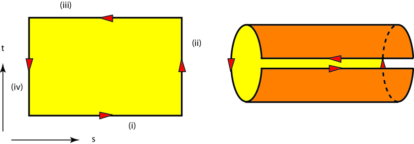
Indeed, since the loop is contractible the sum of the terms is zero. The individual terms along the boundary components are found as follows, see Figure 6.1: (i) for $-T\leq s\leq T$, it holds that $\Psi(s,0)={\rm Id}$, and thus ${\rm gr}(\Psi(s,0))=\Delta$ and $\mu({\rm gr}(\Psi(s,0)),\Delta_{\sigma})=\mu(\Delta,\Delta_{\sigma})$; (ii) for $0\leq t\leq 1$, we have $\Psi(T,t)=\Psi_{+}(t)$, and therefore $\mu({\rm gr}(\Psi_{+}),\Delta_{\sigma})=\mu_{\sigma}(\Psi_{+},1)$; (iii) for $-T\leq s\leq T$ (opposite direction) the previous calculations with the crossing form for $L(s)$ show that $\mu({\rm gr}(\Psi(s,1)),\Delta_{\sigma})=\mu_{\rm spec}(L)$; (iv) for $0\leq t\leq 1$ (opposite direction), it holds that $\Psi(-T,t)=\Psi_{-}(t)$, and therefore $\mu({\rm gr}(\Psi_{-}),\Delta_{\sigma})=\mu_{\sigma}(\Psi_{-},1)$. Since ${\rm ind}~{}D_{L}=-\mu_{\rm spec}(L)$ we obtain

$${\rm ind}~{}D_{L}={\rm ind}~{}\partial_{K,\Delta_{\sigma}}=\mu_{\sigma}(\Psi_{-},1)-\mu_{\sigma}(\Psi_{+},1)+\mu(\Delta,\Delta_{\sigma}).$$

Since $\Delta_{\sigma}$ and $\Delta$ are both constant Lagrangian curves, it follows that $\mu(\Delta,\Delta_{\sigma})=0$, which concludes the proof of the Theorem. $\Box$

We recall from Section 4 that the Hamiltonian for multi-strand braids is defined as $\overline{H}(t,\textsc{x}(t))=\sum_{k=1}^{n}H(t,x^{k}(t))$. The linearization around a braid x is given by

$$L_{\textsc{x}}\stackrel{{\scriptstyle\mbox{\tiny{\raisebox{0.0pt}[0.0pt][0.0pt]{def}}}}}{{=}}-d^{2}{\mathscr{L}}_{H}(\textsc{x})=\overline{J}_{0}\frac{d}{dt}+d^{2}\overline{H}(t,\textsc{x}).$$ (6.3.1)

Define the symplectic path $\Psi:[0,1]\to{\rm Sp}(2n,{\mathbb{R}})$ by

$$\frac{d\Psi}{dt}-\overline{J}_{0}d^{2}\overline{H}(t,\textsc{x}(t))\Psi=0,\qquad\Psi(0)=\text{Id}.$$ (6.3.2)

For convenience we write $K(t)=d^{2}\overline{H}(t,\textsc{x}(t))$, so that the linearized equation becomes $\frac{d}{dt}\Psi-\overline{J}_{0}K(t)\Psi=0$.

$\blacktriangleleft$ 6.3 Lemma. If $\det\bigl{(}\Psi(1)-\bm{\sigma}\bigr{)}\neq 0$, then $\mu_{\sigma}(\Psi,1)$ is an integer. $\blacktriangleright$

Proof.    Since crossings between ${\rm gr}(\Psi)$ and $\Delta_{\sigma}$ occur when $\det\bigl{(}\Psi(t)-\bm{\sigma}\bigr{)}=0$, the only endpoint that may lead to a non-integer contribution is the starting point. There the crossing form is, as in (6.2.2), given by

$$\Gamma({\rm gr}(\Psi),\Delta_{\sigma},0)(\xi^{\sigma})=\langle\xi,\bm{\sigma}^{T}K(0)\bm{\sigma}\xi\rangle,$$

for all $\xi\in\ker(\Psi(0)-\bm{\sigma})$. The kernel of $\Psi(0)-\bm{\sigma}=\text{Id}-\bm{\sigma}$ is even dimensional, since in coordinates (6.2.1) it is of the form $\ker(\text{Id}_{2n}-\bm{\sigma})=\ker(\text{Id}_{n}-\sigma)\times\ker(\text{Id}_{n}-\sigma).$ Therefore, $\text{sign}~{}\Gamma({\rm gr}(\Psi),\Delta_{\sigma},0)$ is always even, and $\mu_{\sigma}(\Psi,1)$ is an integer. $\Box$

The non-degeneracy condition leads to an integer valued Conley-Zehnder index for braids.

$\blacktriangleleft$ 6.4 Definition.  A stationary braid x is said to be non-degenerate if $\det\bigl{(}\Psi(1)-\bm{\sigma}\bigr{)}\neq 0$. The Conley-Zehnder index of a non-degenerate stationary braid x is defined by $\mu(\textsc{x})\stackrel{{\scriptstyle\mbox{\tiny{\raisebox{0.0pt}[0.0pt][0.0pt]{def}}}}}{{=}}\mu_{\sigma}(\Psi,1)$, where $\sigma\in S_{n}$ is the associated permutation of x. $\blacktriangleright$

$\blacktriangleleft$ 6.5 Remark.  If $\textsc{x}=\{x^{k}(t)\}$ is a stationary non-degenerate braid, then $\mu(\textsc{x})$ can be related to the Morse indices $\mu_{H}(x^{k})$ provided that the matrix norm of $K=d^{2}H(x^{k})$ is not too large, e.g. if $\|K\|<2\pi$. For $\mu_{H}(\textsc{x})\stackrel{{\scriptstyle\mbox{\tiny{\raisebox{0.0pt}[0.0pt][0.0pt]{def}}}}}{{=}}\sum_{k}\mu_{H}(x^{k})$,

$$\mu(\textsc{x})=\mu_{\sigma}(\Psi,1)=\sum_{k}\left(1-\mu_{H}(x^{k})\right)=n-\mu_{H}(\textsc{x}).$$ (6.3.3)

This relation can be useful in some instances for computing Floer homology, see Sect. 11.2. Indeed, in dimension two $\Psi$ satisfies: $\Psi(t)=\exp{\left(J_{0}Kt\right)}$, where $K=d^{2}H(x^{k}(t))$ is a constant matrix. Then $\mu(x^{k})=\mu_{\rm CZ}(\Psi)=1-\mu^{-}(K)$, where $\mu^{-}(K)$ is the number of negative eigenvalues of eigenvalues. The latter equality follows from Thm. 3.3 in [34]. $\blacktriangleright$

7. Transversality and connecting orbit spaces

Central to the analysis of the Cauchy-Riemann equations are various generic non-degeneracy and transversality properties. The first important statement in this direction involves the generic non-degeneracy of critical points.

7.1. Generic properties of critical points

Define ${\rm Crit}_{H}\left([\textsc{x}]{~{}{\rm rel}~{}}\textsc{y}\right)$ to be those critical points in ${\rm Crit}_{H}$ that are contained in the braid class $[\textsc{x}]{~{}{\rm rel}~{}}\textsc{y}$.

$\blacktriangleleft$ 7.1 Proposition.  Let $[\textsc{x}]{~{}{\rm rel}~{}}\textsc{y}$ be a proper relative braid class. Then, for any Hamiltonian $H\in{\mathscr{H}}$, with $\textsc{y}\in{\rm Crit}_{H}(\Omega^{m})$, there exists a $\delta_{*}>0$ such that for any $\delta<\delta_{*}$ there exists a nearby Hamiltonian $H^{\prime}\in{\mathscr{H}}$ satisfying

1. $\|H-H^{\prime}\|_{C^{\infty}}<\delta$;

2. $\textsc{y}\in{\rm Crit}_{H^{\prime}}(\Omega^{m})$,

such that ${\rm Crit}_{H^{\prime}}\left([\textsc{x}]{~{}{\rm rel}~{}}\textsc{y}\right)$ consists of only finitely many non-degenerate critical points for the action ${\mathscr{L}}_{H^{\prime}}$. $\blacktriangleright$

We say that the property that ${\rm Crit}_{H}\left([\textsc{x}]{~{}{\rm rel}~{}}\textsc{y}\right)$ consists of only non-degenerate critical points is a generic property, and is satisfied by generic Hamiltonians in the above sense.

Proof.    Given $H\in{\mathscr{H}}$ we start off with defining a class of perturbations. For a braid $\textsc{y}\in\Omega^{m}$, define the tubular neighborhood $N_{\epsilon}(\textsc{y})$ of y in ${\mathbb{R}}/{\mathbb{Z}}\times{\mathbb{D}}^{2}$ by :

$$N_{\epsilon}(\textsc{y})=\bigcup_{\stackrel{{\scriptstyle k=1,\cdots,m}}{{t\in[0,1]}}}B_{\epsilon}(y^{k}(t)).$$

If $\epsilon>0$ is sufficiently small, then a neighborhood $N_{\epsilon}(\textsc{y})$ consists of $m$ disjoint cylinders. Let $D_{\epsilon}=\{x\in{\mathbb{D}}^{2}~{}|~{}1-\epsilon<|x|\leq 1\}$ be a small neighborhood of the boundary, and define

$$A_{\epsilon}=N_{\epsilon}(\textsc{y})\cup\bigl{(}{\mathbb{R}}/{\mathbb{Z}}\times D_{\epsilon}\bigr{)},\quad A_{\epsilon}^{c}=\bigl{(}{\mathbb{R}}/{\mathbb{Z}}\times{\mathbb{D}}^{2}\bigr{)}\backslash A_{\epsilon}.$$

Let ${\mathscr{T}}^{J,H}([\textsc{x}]{~{}{\rm rel}~{}}\textsc{y})$ represent the paths in the cylinder traced out by the elements of ${\mathscr{S}}^{J,H}([\textsc{x}]{~{}{\rm rel}~{}}\textsc{y})$:

$${\mathscr{T}}^{J,H}([\textsc{x}]{~{}{\rm rel}~{}}\textsc{y})\stackrel{{\scriptstyle\mbox{\tiny{\raisebox{0.0pt}[0.0pt][0.0pt]{def}}}}}{{=}}\bigl{\{}(t,x^{k}(t))\bigm{|}1\leq k\leq n,\,t\in[0,1],\,\textsc{x}\in{\mathscr{S}}^{J,H}([\textsc{x}]{~{}{\rm rel}~{}}\textsc{y})\bigr{\}}.$$

Since $[\textsc{x}]{~{}{\rm rel}~{}}\textsc{y}$ is proper, there exists an $\epsilon_{*}>0$, such that for all $\epsilon\leq\epsilon_{*}$ it holds that ${\mathscr{T}}^{J,H}([\textsc{x}]{~{}{\rm rel}~{}}\textsc{y})\subset{\rm int}(A_{2\epsilon}^{c})$. Now fix $\epsilon\in(0,\epsilon_{*}]$. On $C^{\infty}({\mathbb{R}}/{\mathbb{Z}}\times{\mathbb{D}}^{2};{\mathbb{R}})$ we define the norm

$$\|{h}\|_{C^{\infty}}\stackrel{{\scriptstyle\mbox{\tiny{\raisebox{0.0pt}[0.0pt][0.0pt]{def}}}}}{{=}}\sum_{k=0}^{\infty}\epsilon_{k}\|{h}\|_{C^{k}},$$

for a sufficiently fast decaying sequence $\epsilon_{k}>0$, such that $C^{\infty}$ equipped with this norm is a separable Banach space, dense in $L^{2}$. Let

$${\mathscr{V}}_{\epsilon} \stackrel{{\scriptstyle\mbox{\tiny{\raisebox{0.0pt}[0.0pt][0.0pt]{def}}}}}{{=}} \{h\in C^{\infty}({\mathbb{R}}/{\mathbb{Z}}\times{\mathbb{D}}^{2};{\mathbb{R}})~{}|~{}\text{supp}\,h\subset A^{c}_{\epsilon}\},$$

$${\mathscr{V}}_{\delta,\epsilon} \stackrel{{\scriptstyle\mbox{\tiny{\raisebox{0.0pt}[0.0pt][0.0pt]{def}}}}}{{=}} \{h\in{\mathscr{V}}_{\epsilon}~{}|~{}\|h\|_{C^{\infty}}<\delta\},$$

and consider Hamiltonians of the form $H^{\prime}=H+h_{\delta}\in{\mathscr{H}}$, with $h_{\delta}\in{\mathscr{V}}_{\delta,\epsilon}$. Then, by construction, $\textsc{y}\in{\rm Crit}_{H^{\prime}}(\overline{\Omega}^{m})$, and by Proposition 5.3 the set ${\mathscr{S}}^{J,H^{\prime}}([\textsc{x}]{~{}{\rm rel}~{}}\textsc{y})$ is compact and isolated in the proper braid class $[\textsc{x}]{~{}{\rm rel}~{}}\textsc{y}$ for all perturbation $h_{\delta}\in{\mathscr{V}}_{\delta,\epsilon}$. A straightforward compactness argument using the compactness result of Proposition 5.3 shows that ${\mathscr{T}}^{J,H+h_{\delta}}([\textsc{x}]{~{}{\rm rel}~{}}\textsc{y})$ converges to ${\mathscr{T}}^{J,H}([\textsc{x}]{~{}{\rm rel}~{}}\textsc{y})$ in the Hausdorff metric as $\delta\to 0$. Therefore, there exists a $\delta_{*}>0$, such that ${\mathscr{T}}^{J,H+h_{\delta}}([\textsc{x}]{~{}{\rm rel}~{}}\textsc{y})\subset{\rm int}(A_{2\epsilon}^{c})$, for all $0\leq\delta\leq\delta_{*}$. In particular ${\rm Crit}_{H+h_{\delta,\epsilon}}\subset{\rm int}(A_{2\epsilon}^{c})$, for all $0\leq\delta\leq\delta_{*}$. Now fix $\delta\in(0,\delta_{*}]$.

The Hamilton equations for $H^{\prime}$ are $x_{t}^{k}-J_{0}\nabla H(t,x^{k})-J_{0}\nabla h(t,x)=0$, with periodic boundary conditions in $t$. Define ${\mathscr{U}}_{\epsilon}\subset W^{1,2}_{\sigma}([0,1];{\mathbb{R}}^{2n})$ to be the open subset of functions $\textsc{x}=\{x^{k}\}$ such that $x^{k}(t)\in{\rm int}(A_{2\epsilon}^{c})$ and define the nonlinear mapping

$${\mathcal{G}}:{\mathscr{U}}_{\epsilon}\times{\mathscr{V}}_{\delta,\epsilon}\to L^{2}([0,1];{\mathbb{R}}^{2n}),$$

which represents the above system of equations and boundary conditions. Explicitly,

$${\mathcal{G}}(\textsc{x},h)=\overline{J}_{0}\textsc{x}_{t}+\nabla\overline{H}(t,\textsc{x})+\nabla\overline{h}(t,\textsc{x}),$$

where $\overline{H}(t,\textsc{x})=\sum_{k}H(t,x^{k})$, and likewise for $\overline{h}$. The mapping ${\mathcal{G}}$ is linear in $h$. Since ${\mathcal{G}}$ is defined on ${\mathscr{U}}_{\epsilon}$ and both $H$ and $h$ are of class $C^{\infty}$, the mapping ${\mathcal{G}}$ is of class $C^{1}$. The derivative with respect to variations $(\xi,\delta h)\in W^{1,2}_{\sigma}([0,1];{\mathbb{R}}^{2n})\times{\mathscr{V}}_{\epsilon}$ is given by

$$d{\mathcal{G}}(\textsc{x},h)(\xi,\delta h) = \overline{J}_{0}\xi_{t}+d^{2}\overline{H}(t,\textsc{x})\xi+d^{2}\overline{h}(t,\textsc{x})\xi+\nabla\delta\overline{h}(t,\textsc{x})$$

$$= L_{\textsc{x}}\xi+\nabla\delta\overline{h}(t,\textsc{x}),$$

where $L_{\textsc{x}}=\overline{J}_{0}\frac{d}{dt}+d^{2}\overline{H}(t,\textsc{x})+d^{2}\overline{h}(t,\textsc{x})$, by analogy with Equation (6.3.1). We see that there is a one-to-one correspondence between elements $\Psi$ in the kernel of $L_{\textsc{x}}$ and symplectic paths described by Equation (6.3.2) with $\det\bigl{(}\Psi(1)-\bm{\sigma}\bigr{)}=0$. In other words, the stationary braid x is non-degenerate if and only if $L_{\textsc{x}}$ has trivial kernel.

The operator $L_{\textsc{x}}$ is a self-adjoint operator on $L^{2}([0,1];{\mathbb{R}}^{2n})$ with domain $W^{1,2}_{\sigma}([0,1];{\mathbb{R}}^{2n})$ and is Fredholm with ${\rm ind}(L_{\textsc{x}})=0$. Therefore ${\mathcal{G}}_{h}\stackrel{{\scriptstyle\mbox{\tiny{\raisebox{0.0pt}[0.0pt][0.0pt]{def}}}}}{{=}}{\mathcal{G}}(\cdot,h)$ is a (proper) nonlinear Fredholm operator with

$${\rm ind}({\mathcal{G}}_{h})={\rm ind}(L_{\textsc{x}})=0.$$

Define the set

$${\mathscr{Z}}=\bigl{\{}(\textsc{x},h)\in{\mathscr{U}}_{\epsilon}\times{\mathscr{V}}_{\delta,\epsilon}~{}|~{}{\mathcal{G}}(\textsc{x},h)=0\bigr{\}}={\mathcal{G}}^{-1}(0).$$

We show that $Z$ is a Banach manifold by demonstrating that $d{\mathcal{G}}(\textsc{x},h)$ is surjective for all $(\textsc{x},h)\in Z$. Since $d{\mathcal{G}}(\textsc{x},h)(\xi,\delta h)=L_{\textsc{x}}\xi-\nabla\delta\overline{h}(t,\textsc{x})$, and the (closed) range of $L_{\textsc{x}}$ has finite codimension, we need to show there is a (finite dimensional) complement of $R(L_{\textsc{x}})$ in the image of $\nabla\delta\overline{h}(t,\textsc{x})$. It suffices to show that $\nabla\delta\overline{h}(t,\textsc{x})$ is dense in $L^{2}([0,1];{\mathbb{R}}^{2n})$.

Recall that for any pair $(\textsc{x},h)\in Z$, it holds that $\textsc{x}\in{\rm Crit}_{H^{\prime}}\subset{\rm int}(A_{2\epsilon}^{c})$. As before consider a neighborhood $N_{\epsilon}(\textsc{x})$, so that $N_{\epsilon}(\textsc{x})\subset{\rm int}(A_{\epsilon}^{c})$ and consists of $n$ disjoint cylinders $N_{\epsilon}(x^{k})$. Let $\phi_{\epsilon}^{k}(t,x)\in C_{0}^{\infty}(N_{\epsilon}(x^{k}))$, such that $\phi_{\epsilon}^{k}\equiv 1$ on $N_{\epsilon/2}(x^{k})$. Define, for arbitrary $f^{k}\in C^{\infty}({\mathbb{R}}/{\mathbb{Z}};{\mathbb{R}}^{2})$,

$$(\delta h)(t,x)=\sum_{k=1}^{n}\phi_{\epsilon}^{k}(t,x)\langle f^{k}(t),x\rangle_{L^{2}}.$$

Since $\phi^{k}_{\epsilon}(t,x^{k}(t))\equiv 1$ it holds that $\delta\overline{h}(t,\textsc{x})=\sum_{k=1}^{n}\langle f^{k}(t),x^{k}\rangle_{L^{2}}$ for $\textsc{x}\in{\rm Crit}_{H^{\prime}}$, and therefore the gradient satisfies $\nabla\delta\overline{h}(t,\textsc{x})={\mathbf{f}}=(f^{k})\in C^{\infty}({\mathbb{R}}/{\mathbb{Z}};{\mathbb{R}}^{2n})$. Moreover, $\delta h\in{\mathscr{V}}_{\epsilon}$ by construction, and because $C^{\infty}({\mathbb{R}}/{\mathbb{Z}};{\mathbb{R}}^{2n})$ is dense in $L^{2}([0,1];{\mathbb{R}}^{2n})$ it follows that $d{\mathcal{G}}(\textsc{x},h)$ is surjective.

Consider the projection $\pi:{\mathscr{Z}}\to{\mathscr{V}}_{\delta,\epsilon}$, defined by $\pi(\textsc{x},h)=h$. The projection $\pi$ is a Fredholm operator. Indeed, $d\pi:T_{(\textsc{x},h)}{\mathscr{Z}}\to{\mathscr{V}}_{\epsilon}$, with $d\pi(\textsc{x},h)(\xi,\delta h)=\delta h$, and

$$T_{(\textsc{x},h)}{\mathscr{Z}}=\left\{(\xi,\delta h)\in W^{1,2}_{\sigma}\times{\mathscr{V}}_{\epsilon}~{}|~{}L_{\textsc{x}}\xi-\nabla\delta\overline{h}=0\right\}.$$

From this it follows that ${\rm ind}(d\pi)={\rm ind}(L_{\textsc{x}})=0$. The Sard-Smale Theorem implies that the set of perturbations $h\in{\mathscr{V}}_{\delta,\epsilon}^{\rm reg}\subset{\mathscr{V}}_{\delta,\epsilon}$ for which $h$ is a regular value of $\pi$ is an open and dense subset. It remains to show that $h\in{\mathscr{V}}_{\delta,\epsilon}^{\rm reg}$ yields that $L_{\textsc{x}}$ is surjective. Let $h\in{\mathscr{V}}_{\delta,\epsilon}^{\rm reg}$, and $(\textsc{x},h)\in Z$, then $d{\mathcal{G}}(\textsc{x},h)$ is surjective, i.e., for any $\zeta\in L^{2}([0,1];{\mathbb{R}}^{2n})$ there are $(\xi,\delta h)$ such that $d{\mathcal{G}}(\textsc{x},h)(\xi,\delta h)=\zeta$. On the other hand, since since $h$ is a regular value for $\pi$, there exists a $\widehat{\xi}$ such that $d\pi(\textsc{x},h)(\widehat{\xi},\delta h)=\delta h$ , $(\widehat{\xi},\delta h)\in T_{(\textsc{x},h)}{\mathscr{Z}}$, i.e. $L_{\textsc{x}}\widehat{\xi}-\nabla\delta\overline{h}=0$. Now

$$L_{\textsc{x}}(\xi-\widehat{\xi}) = d{\mathcal{G}}(\textsc{x},h)(\xi-\widehat{\xi},0)$$

$$= d{\mathcal{G}}(\textsc{x},h)\bigl{(}(\xi,\delta h)-(\widehat{\xi},\eta)\bigr{)}=\zeta-0=\zeta,$$

which proves that for all $h\in{\mathscr{V}}_{\delta,\epsilon}^{\rm reg}$ the operator $L_{\textsc{x}}$ is surjective, and hence also injective, implying that x is non-degenerate. $\Box$

For $\textsc{x}_{\pm}\in{\rm Crit}_{H}$, let ${\mathscr{M}}_{\textsc{x}_{-},\textsc{x}_{+}}^{J,H}([\textsc{x}]{~{}{\rm rel}~{}}\textsc{y})$ be the space of all bounded solutions in $\textsc{u}\in{\mathscr{M}}^{J,H}([\textsc{x}]{~{}{\rm rel}~{}}\textsc{y})$ such that $\lim_{s\to\pm\infty}\textsc{u}(s,\cdot)=\textsc{x}_{\pm}(\cdot)$, i.e., connecting orbits in the relative braid class $[\textsc{x}]{~{}{\rm rel}~{}}\textsc{y}$. If $\textsc{x}_{-}=\textsc{x}_{+}$, then the set consists of just this one critical point. The space ${\mathscr{S}}_{\textsc{x}_{-},\textsc{x}_{+}}^{J,H}([\textsc{x}]{~{}{\rm rel}~{}}\textsc{y})$, as usual, consists of the corresponding trajectories.

$\blacktriangleleft$ 7.2 Lemma.  Let $[\textsc{x}]{~{}{\rm rel}~{}}\textsc{y}$ be a proper braid class and let $H\in{\mathscr{H}}$ be a generic Hamiltonian. Then

$${\mathscr{M}}^{J,H}([\textsc{x}]{~{}{\rm rel}~{}}\textsc{y})\subset\bigcup_{\textsc{x}_{\pm}\in{\rm Crit}_{H}}{\mathscr{M}}_{\textsc{x}_{-},\textsc{x}_{+}}^{J,H}([\textsc{x}]{~{}{\rm rel}~{}}\textsc{y}),$$

where ${\rm Crit}_{H}={\rm Crit}_{H}([\textsc{x}]{~{}{\rm rel}~{}}\textsc{y})$. $\blacktriangleright$

See [32] for a detailed proof.

$\blacktriangleleft$ 7.3 Corollary.  Let $[\textsc{x}]{~{}{\rm rel}~{}}\textsc{y}$ be a proper relative braid class and let $H$ be a generic Hamiltonian with $\textsc{y}\in{\rm Crit}_{H}(\overline{\Omega}^{m})$. Then the space of bounded solutions is given by the union ${\mathscr{M}}^{J,H}([\textsc{x}]{~{}{\rm rel}~{}}\textsc{y})=\bigcup_{\textsc{x}_{\pm}\in{\rm Crit}_{H}}{\mathscr{M}}_{\textsc{x}_{-},\textsc{x}_{+}}^{J,H}([\textsc{x}]{~{}{\rm rel}~{}}\textsc{y})$. $\blacktriangleright$

Proof.    The key observation is that since $\textsc{x}_{\pm}{~{}{\rm rel}~{}}\textsc{y}\in[\textsc{x}]{~{}{\rm rel}~{}}\textsc{y}$, also $\textsc{u}(s,\cdot){~{}{\rm rel}~{}}\textsc{y}\in[\textsc{x}]{~{}{\rm rel}~{}}\textsc{y}$, for all $s\in{\mathbb{R}}$ (the crossing number cannot change). Therefore, any $\textsc{u}\in{\mathscr{M}}_{\textsc{x}_{-},\textsc{x}_{+}}^{J,H}([\textsc{x}]{~{}{\rm rel}~{}}\textsc{y})$ is contained in $[\textsc{x}]{~{}{\rm rel}~{}}\textsc{y}$, and thus ${\mathscr{M}}_{\textsc{x}_{-},\textsc{x}_{+}}^{J,H}([\textsc{x}]{~{}{\rm rel}~{}}\textsc{y})\subset{\mathscr{M}}^{J,H}([\textsc{x}]{~{}{\rm rel}~{}}\textsc{y})$. The remainder of the proof follows from Lemma 7.1. $\Box$

Note that the sets ${\mathscr{M}}_{\textsc{x}_{-},\textsc{x}_{+}}^{J,H}([\textsc{x}]{~{}{\rm rel}~{}}\textsc{y})$ are not necessarily compact in $\overline{\Omega}^{n}$. The following corollary gives a more precise statement about the compactness of the spaces ${\mathscr{M}}_{\textsc{x}_{-},\textsc{x}_{+}}^{J,H}([\textsc{x}]{~{}{\rm rel}~{}}\textsc{y})$, which will be referred to as geometric convergence.

$\blacktriangleleft$ 7.4 Corollary.  Let $[\textsc{x}]{~{}{\rm rel}~{}}\textsc{y}$ be a proper relative braid class and $H$ be a generic Hamiltonian with $\textsc{y}\in{\rm Crit}_{H}(\overline{\Omega}^{m})$. Then for any sequence $\{\textsc{u}_{n}\}\subset{\mathscr{M}}_{\textsc{x}_{-},\textsc{x}_{+}}^{J,H}([\textsc{x}]{~{}{\rm rel}~{}}\textsc{y})$ (along a subsequence) there exist stationary braids $\textsc{x}^{i}\in{\rm Crit}_{H}([\textsc{x}]{~{}{\rm rel}~{}}\textsc{y})$, $i=0,\dots,m$, orbits $\textsc{u}^{i}\in{\mathscr{M}}_{\textsc{x}^{i},\textsc{x}^{i-1}}^{J,H}([\textsc{x}]{~{}{\rm rel}~{}}\textsc{y})$ and times $s_{n}^{i}$, $i=1,\dots,m$, such that

$$\textsc{u}_{n}(\cdot+s_{n}^{i},\cdot)\longrightarrow\textsc{u}^{i},\quad n\to\infty,$$

in $C^{r}_{\rm loc}({\mathbb{R}}\times{\mathbb{R}}/{\mathbb{Z}})$, for any $r\geq 1$. Moreover, $\textsc{x}^{0}=\textsc{x}_{+}$ and $\textsc{x}^{m}=\textsc{x}_{-}$ and ${\mathscr{L}}_{H}(\textsc{x}^{i})>{\mathscr{L}}_{H}(\textsc{x}^{i-1})$ for $i=1,\dots,m$. The sequence $\textsc{u}_{n}$ is said to geometrically converge to the broken trajectory $(\textsc{u}^{1},\dots,\textsc{u}^{m})$. $\blacktriangleright$

See, again, [32] for a proof.

7.2. Generic properties for connecting orbits

As for critical points, non-degeneracy can also be defined for connecting orbits. This closely follows the ideas in the previous subsection. Set $W^{1,p}_{\sigma}=W^{1,p}_{\sigma}({\mathbb{R}}\times[0,1];{\mathbb{R}}^{2n})$ and $L^{p}=L^{p}({\mathbb{R}}\times[0,1];{\mathbb{R}}^{2n})$.

Let $\textsc{x}_{-},\textsc{x}_{+}\in{\rm Crit}_{H}(\overline{\Omega}^{n})$ be non-degenerate stationary braids. A connecting orbit $\textsc{u}\in{\mathscr{M}}_{\textsc{x}_{-},\textsc{x}_{+}}^{J,H}$ is said to be non-degenerate, or transverse, if the linearized Cauchy-Riemann operator

$${\partial\over\partial s}-\overline{J}{\partial\over\partial t}+\overline{J}\overline{J}_{0}d^{2}\overline{H}(t,\textsc{u}(s,t)):~{}W^{1,p}_{\sigma}\to L^{p},$$

is a surjective operator (for all $1<p<\infty$).

As before we equip $C^{\infty}({\mathbb{R}}/{\mathbb{Z}}\times{\mathbb{D}}^{2};{\mathbb{R}})$ with a Banach structure, cf. Sect. 7.1.

$\blacktriangleleft$ 7.5 Proposition.  Let $[\textsc{x}]{~{}{\rm rel}~{}}\textsc{y}$ be a proper relative braid class, and $H\in{\mathscr{H}}$ be a generic Hamiltonian such that $\textsc{y}\in{\rm Crit}_{H}(\overline{\Omega}^{m})$. Then, there exists a $\delta_{*}>0$ such that for any $\delta\leq\delta_{*}$ there exists a nearby Hamiltonian $H^{\prime}\in{\mathscr{H}}$ with $\|H-H^{\prime}\|_{C^{\infty}}<\delta$ and $\textsc{y}\in{\rm Crit}_{H^{\prime}}(\overline{\Omega}^{m})$ such that

1. ${\rm Crit}_{H^{\prime}}([\textsc{x}]{~{}{\rm rel}~{}}\textsc{y})={\rm Crit}_{H}([\textsc{x}]{~{}{\rm rel}~{}}\textsc{y})$ and consists of only non-degenerate stationary points for the action ${\mathscr{L}}_{H^{\prime}}$;

and for any pair $\textsc{x}_{-},\textsc{x}_{+}\in{\rm Crit}_{H^{\prime}}([\textsc{x}]{~{}{\rm rel}~{}}\textsc{y})$

1. ${\mathscr{S}}^{J,H^{\prime}}_{\textsc{x}_{-},\textsc{x}_{+}}([\textsc{x}]{~{}{\rm rel}~{}}\textsc{y})$ is isolated in $[\textsc{x}]{~{}{\rm rel}~{}}\textsc{y}$;

2. ${\mathscr{M}}_{\textsc{x}_{-},\textsc{x}_{+}}^{J,H^{\prime}}([\textsc{x}]{~{}{\rm rel}~{}}\textsc{y})$ consists of non-degenerate connecting orbits;

3. ${\mathscr{M}}^{J,H^{\prime}}_{\textsc{x}_{-},\textsc{x}_{+}}([\textsc{x}]{~{}{\rm rel}~{}}\textsc{y})$ are smooth manifolds without boundary and

$$\dim{\mathscr{M}}^{J,H^{\prime}}_{\textsc{x}_{-},\textsc{x}_{+}}([\textsc{x}]{~{}{\rm rel}~{}}\textsc{y})=\mu(\textsc{x}_{-})-\mu(\textsc{x}_{+}),$$

where $\mu$ is the Conley-Zehnder index defined in Definition 6.3. $\blacktriangleright$

Proof.    Since $[\textsc{x}]{~{}{\rm rel}~{}}\textsc{y}$ is a proper braid class it follows from Proposition 5.3 that ${\mathscr{S}}^{J,H^{\prime}}_{\textsc{x}_{-},\textsc{x}_{+}}$ is isolated in $[\textsc{x}]{~{}{\rm rel}~{}}\textsc{y}$ for any $H^{\prime}\in{\mathscr{H}}$ provided $\textsc{y}\in{\rm Crit}_{H^{\prime}}$.

As for the transversality properties we follow Salamon and Zehnder [34], where perturbations in ${\mathbb{R}}^{2n}$ are considered. We adapt the proof for Hamiltonians in ${\mathbb{R}}^{2}$. The proof is similar in spirit to the genericity of critical points.

As in the proof of Proposition 7.1 we denote by ${\mathscr{V}}_{\epsilon}$ the set of perturbations $h\in C^{\infty}({\mathbb{R}}/{\mathbb{Z}}\times{\mathbb{D}}^{2};{\mathbb{R}})$ whose support is bounded away from $(t,\textsc{y}(t))$, $(t,\textsc{x}_{\pm}(t))$ and $\partial{\mathbb{D}}^{2}$ (this yields a corresponding set $A_{\epsilon}$ as in the proof of Proposition 7.1). If we choose $h\in{\mathscr{V}}_{\delta,\epsilon}$ there exists a $\delta_{*}$ such that ${\rm Crit}_{H^{\prime}}([\textsc{x}]{~{}{\rm rel}~{}}\textsc{y})={\rm Crit}_{H}([\textsc{x}]{~{}{\rm rel}~{}}\textsc{y})$ and consists of only non-degenerate stationary points for the action ${\mathscr{L}}_{H^{\prime}}$. For details of this construction we refer to the proof of Proposition 7.1.

Define the Cauchy-Riemann operator

$${\mathcal{G}}(\textsc{u},{h})=\textsc{u}_{s}-\overline{J}\textsc{u}_{t}+\overline{J}\overline{J}_{0}\nabla\overline{H}(t,\textsc{u})+\overline{J}\overline{J}_{0}\nabla\overline{h}(t,\textsc{u}).$$

Based on the a priori regularity of bounded solutions of the Cauchy-Riemann equations we define for $2<p<\infty$ the affine spaces

$${\mathscr{U}}^{1,p}(\textsc{x}_{-},\textsc{x}_{+})\stackrel{{\scriptstyle\mbox{\tiny{\raisebox{0.0pt}[0.0pt][0.0pt]{def}}}}}{{=}}\bigl{\{}\gamma+\xi~{}|~{}\xi\in W^{1,p}_{\sigma}({\mathbb{R}}\times[0,1];{\mathbb{R}}^{2n})\bigr{\}},$$ (7.2.1)

and balls ${\mathscr{U}}_{\varepsilon}^{1,p}=\{\textsc{u}\in{\mathscr{U}}^{1,p}\,|\,\|\xi\|_{W^{1,p}_{\sigma}}<\epsilon\}$, where $\gamma(s,t)\in C^{2}\bigl{(}{\mathbb{R}}\times[0,1];({\mathbb{D}}^{2})^{n}\bigr{)}$ is a fixed connecting path such that $\lim_{s\rightarrow\pm\infty}\gamma(s,\cdot)=\textsc{x}_{\pm}$ and $\gamma(s,t)\in{\rm int}({\mathbb{D}}^{2})^{n}$ for all $(s,t)\in{\mathbb{R}}\times[0,1]$. Therefore, for $p>2$, functions $\textsc{u}\in\mathcal{U}_{\epsilon}^{1,p}(\textsc{x}_{-},\textsc{x}_{+})$ satisfy the limits $\lim_{s\rightarrow\pm\infty}\textsc{u}(s,\cdot)=\textsc{x}_{\pm}$ and if $\epsilon>0$ is chosen sufficiently small then also $\textsc{u}(s,t)\in{\rm int}({\mathbb{D}}^{2})^{n}$ for all $(s,t)\in{\mathbb{R}}\times[0,1]$. The mapping

$${\mathcal{G}}:{\mathscr{U}}_{\epsilon}^{1,p}(\textsc{x}_{-},\textsc{x}_{+})\times{\mathscr{V}}_{\delta,\epsilon}\rightarrow L^{p}({\mathbb{R}}\times[0,1];{\mathbb{R}}^{2n}),$$

is smooth. Define

$${\mathscr{Z}}_{\textsc{x}_{-},\textsc{x}_{+}}\stackrel{{\scriptstyle\mbox{\tiny{\raisebox{0.0pt}[0.0pt][0.0pt]{def}}}}}{{=}}\bigl{\{}(\textsc{u},{h})\in\mathcal{U}_{\epsilon}^{1,p}(\textsc{x}_{-},\textsc{x}_{+})\times{\mathscr{V}}_{\delta,\epsilon}\ |\ {\mathcal{G}}(\textsc{u},{h})=0\bigr{\}}={\mathcal{G}}^{-1}(0),$$

which is Banach manifold provided that $d{\mathcal{G}}(\textsc{u},{h})$ is onto on for all $(\textsc{u},{h})\in{\mathscr{Z}}_{\textsc{x}_{-},\textsc{x}_{+}}$, where

$$d{\mathcal{G}}(\textsc{u},{h})(\xi,\delta{h})=d_{1}{\mathcal{G}}(\textsc{u},\delta{h})\xi+\overline{J}\overline{J}_{0}\nabla\overline{\delta{h}}.$$

Assume that $d{\mathcal{G}}(\textsc{u},{h})$ is not onto. Then there exists a non-zero function $\eta\in L^{q}$ which annihilates the range of $d{\mathcal{G}}(\textsc{u},{h})$ and thus also the range of $d_{1}{\mathcal{G}}(\textsc{u},{h})$, which is a Fredholm operator of index $\mu(\textsc{x}_{-})-\mu(\textsc{x}_{+})$; see Proposition 6.3. The relation $\langle d_{1}{\mathcal{G}}(\textsc{u},{h})(\xi),\eta\rangle=0$ for all $\xi$ implies that

$$d_{1}{\mathcal{G}}(\textsc{u},{h})^{*}\eta=-\eta_{s}-\overline{J}\eta_{t}+\overline{J}\overline{J}_{0}d^{2}\overline{H}(t,\textsc{u})\eta=0.$$

Since $\langle d{\mathcal{G}}(\textsc{u},{h})(\xi,\delta{h}),\eta\rangle=0$ it follows that

$$\int_{-\infty}^{\infty}\int_{0}^{1}\langle\eta(s,t),\overline{J}\overline{J}_{0}\nabla\delta\overline{{h}}\rangle_{{\mathbb{R}}^{2n}}dtds=0,\qquad\forall\delta{h}.$$ (7.2.2)

Due to the assumptions on ${h}$ and $H$, the regularity theory for the linear Cauchy-Riemann operator implies that $\eta$ is smooth. It remains to show that no such non-zero function $\eta$ exists.

Step $1$: The function $\eta$ satisfies the following perturbed Laplace’s equation: $\Delta\eta=\partial_{\overline{J}}\bar{\partial}_{\overline{J}}\eta=\partial_{\overline{J}}\overline{J}\overline{J}_{0}d^{2}\overline{H}(t,\textsc{u})\eta$. If at some $(s_{0},t_{0})$ all derivatives of $\eta$ vanish, it follows from Aronszajn’s unique continuation [5] that $\eta\equiv 0$ is a neighborhood of $(s_{0},t_{0})$. Therefore $\eta(s,t)\neq 0$ for almost all $(s,t)\in{\mathbb{R}}\times[0,1]$.

Step $2$: The vectors $\eta(s,t)$ and $\textsc{u}_{s}(s,t)$ are linearly dependent for all $s$ and $t$. Suppose not, then these vector are linearly independent at some point $(s_{0},t_{0})$. By Theorem 8.2 in [34] we may assume without loss of generality that $\textsc{u}_{s}(s_{0},t_{0})\not=0$ and $\textsc{u}(s_{0},t_{0})\not=\textsc{x}_{\pm}(t_{0})$ — a regular point. We now follow the arguments as in the proof of Theorem 8.4 in [34] with some modifications. Since $(s_{0},t_{0})$ is a regular point there exists a small neighborhood $U_{0}=I_{t_{0}}\times U_{x^{1}}\times\dots\times U_{x^{n}},$ such that $V_{0}=\{(s,t)~{}|~{}(t,\textsc{u}(s,t))\in U_{0}\}$ is a neighborhood $V_{0}$ of $(s_{0},t_{0})$ and $U_{0}\cap A_{\epsilon}=\varnothing$. The sets $U_{x^{k}}$ are neighborhoods of $u^{k}(s_{0},t_{0})$ and have the important property that $U_{x^{k}}\cap U_{x^{k^{\prime}}}=\varnothing$ for all $k\not=k^{\prime}$. The proof in [34] shows that the map $(s,t)\mapsto(t,\textsc{u}(s,t))$ from $V_{0}$ to $U_{0}$ is a diffeomorphism. By choosing $V_{0}$ small enough $\textsc{u}_{s}$ and $\eta$ are linearly independent on $V_{0}$. As in [34] this yields the existence of coordinates $\phi_{t}:({\mathbb{D}}^{2})^{n}\to{\mathbb{R}}^{2n}$ in a neighborhood $(t_{0},\textsc{u}(s_{0},t_{0}))\in U_{0}$ such that

$$\phi_{t}(\textsc{u}(s,t))=(s-s_{0},0,\dots,0),\qquad d\phi_{t}(\textsc{u}(s,t))\eta(s,t)=(0,1,0,\dots,0).$$

Define $g:{\mathbb{R}}^{2n}\times{\mathbb{S}}^{1}\rightarrow{\mathbb{R}}$ via $g(y_{1},\dots,y_{2n},t)=\beta(t-t_{0})\beta(y_{1})\beta(y_{2})y_{2}$, where $\beta\geq 0$ is a $C^{\infty}$ cutoff function such that $\beta=1$ on a ball centered at zero $B_{\delta_{1}}(0)$ for sufficiently small positive $\delta_{1}$ and $\beta=0$ outside of $B_{2\delta_{1}}(0)$. We define a Hamiltonian $\chi:{\mathbb{S}}^{1}\times({\mathbb{D}}^{2})^{n}\rightarrow{\mathbb{R}}$ via $\chi(t,x_{1},\dots,x_{2n})=g(\phi(x_{1},\dots,x_{2n}),t)$. By construction $\chi$ vanishes outside $U_{0}$, $\chi(t,\textsc{u}(s,t))=g((s-s_{0},0,\dots,0),t)=0$, and $d\chi(t,\textsc{u}(s,t))\eta(s,t)=\beta(s-s_{0})\beta(t-t_{0})$ for all $(s,t)\in V_{0}$. In order to have an admissible perturbation we need a Hamiltonian $\delta h\in{\mathscr{V}}_{\epsilon}$ such that $\chi=\delta\overline{h}$. Since $\chi$ vanishes outside $U_{0}$ and since $U_{x^{k}}\cap U_{x^{k^{\prime}}}=\varnothing$ for all $k\not=k^{\prime}$ we can solve this equation. Set $(\delta h)(t,u^{k}(s_{0},t))=\chi(t,\textsc{u}(s_{0},t_{0}))/n$ and define $\delta h$ on the disjoint set $U_{x^{k}}$ as follows:

$$(\delta h)(t,x^{k})=\chi(t,u^{1}(s_{0},t),\dots,x^{k},\dots,u^{n}(s_{0},t))-\frac{n-1}{n}\chi(t,\textsc{u}(s_{0},t)).$$

Since the sets $U_{x^{k}}$ are disjoint $\delta h$ is well-defined ${\mathbb{S}}^{1}\times{\mathbb{D}}^{2}$ and zero outside $I_{t_{0}}\times(\cup_{k}U_{x^{k}})$. With this choice of perturbation $\delta h$ the integral in Equation (7.2.2) is non-zero which contradicts the assumption on $\eta$.

The remaining steps are identical to those in the proof of Theorem 8.4 in [34]: we outline these for completeness.

Step $3$: The previous step implies the existence of a function $\lambda:{\mathbb{R}}\times[0,1]\rightarrow{\mathbb{R}}$ such that $\eta(s,t)=\lambda(s,t)\frac{\partial\textsc{u}}{\partial s}(s,t)$, for all $s,t$ for which $\eta(s,t)\not=0$. Using a contradiction argument with respect to Equation (7.2.2) yields $\frac{\partial\lambda}{\partial s}(s,t)=0$, for almost all $(s,t)$. In particular we obtain that $\lambda$ is $s$-independent and we can assume that $\lambda(t)\geq\delta>0$ for all $t\in[0,1]$ (invoking again unique continuation).

Step $4$: This final step provides a contradiction to the assumption that $d{\mathcal{G}}$ is not onto. It holds that

$$\int_{0}^{1}\left\langle\frac{\partial\textsc{u}}{\partial s}(s,t),\eta(s,t)\right\rangle dt=\int_{0}^{1}\lambda(t)\left|\frac{\partial\textsc{u}}{\partial s}(s,t)\right|^{2}dt\geq\delta\int_{0}^{1}\left|\frac{\partial\textsc{u}}{\partial s}(s,t)\right|^{2}dt>0.$$

The functions $\textsc{u}_{s}$ and $\eta$ satisfy the equations $d_{1}{\mathcal{G}}(\textsc{u},{h})\textsc{u}_{s}=0,\quad d_{1}{\mathcal{G}}(\textsc{u},{h})^{*}\eta=0$, respectively. From these equations we can derive expressions for $\textsc{u}_{ss}$ and $\eta_{s}$, from which:

$$\frac{d}{ds}\int_{0}^{1}\left\langle\frac{\partial\textsc{u}}{\partial s}(s,t),\eta(s,t)\right\rangle dt=0.$$

Combining this with the previous estimate yields that $\int_{-\infty}^{\infty}\int_{0}^{1}|\textsc{u}_{s}(s,t)|^{2}dt=\infty$, which, combined with the compactness properties, contradicts the fact that $\textsc{u}\in{\mathscr{M}}_{\textsc{x}_{-},\textsc{x}_{+}}$; thus $d{\mathcal{G}}(\textsc{u},{h})$ is onto for all $(\textsc{u},{h})\in{\mathscr{Z}}_{\textsc{x}_{-},\textsc{x}_{+}}$.

We can now apply the Sard-Smale theorem as in the proof of Proposition 7.1. The only difference here is that application of the Sard-Smale requires $(\mu(\textsc{x}_{-})-\mu(\textsc{x}_{+})+1)$-smoothness of ${\mathcal{G}}$ which is guaranteed by the smoothness of y, $H$ and ${h}$. $\Box$

We can label a Hamiltonian to be generic now if both ${\rm Crit}_{H}([\textsc{x}]{~{}{\rm rel}~{}}\textsc{y})$ and ${\mathscr{M}}_{\textsc{x}_{-}.\textsc{x}_{+}}([\textsc{x}]{~{}{\rm rel}~{}}\textsc{y})$, $\textsc{x}_{\pm}\in{\rm Crit}_{H}([\textsc{x}]{~{}{\rm rel}~{}}\textsc{y})$, are non-degenerate. The terminology ‘generic’ is justified since by the taken finitely many intersections for the different pairs $\textsc{x}_{\pm}$ we obtain a dense set of Hamiltonian, denoted by ${\mathscr{H}}_{\rm reg}$. For generic Hamiltonians $H\in{\mathscr{H}}_{\rm reg}$ the convergence of Corollary 7.1 can be extended with estimates on the Conley-Zehnder indices of the stationary braids.

$\blacktriangleleft$ 7.6 Corollary.  Let $[\textsc{x}]{~{}{\rm rel}~{}}\textsc{y}$ be a proper relative braid class and $H\in{\mathscr{H}}_{\rm reg}$ be a generic Hamiltonian with $\textsc{y}\in{\rm Crit}_{H}(\overline{\Omega}^{m})$. If $\textsc{u}_{n}$ geometrically converges to the broken trajectory $(\textsc{u}^{1},\dots,\textsc{u}^{m})$, with $\textsc{u}^{i}\in{\mathscr{M}}_{\textsc{x}^{i},\textsc{x}^{i-1}}^{J,H}([\textsc{x}]{~{}{\rm rel}~{}}\textsc{y})$, $i=1,\dots,m$ and $\textsc{x}^{i}\in{\rm Crit}_{H}([\textsc{x}]{~{}{\rm rel}~{}}\textsc{y})$, $i=0,\dots,m$, then

$$\mu(\textsc{x}^{i})>\mu(\textsc{x}^{i-1}),$$

for $i=1,\dots,m$. $\blacktriangleright$

Proof.    See [32] for a detailed proof of this statement. $\Box$

Since Proposition 7.2 provides a dense set of Hamiltonians ${\mathscr{H}}_{\rm reg}$ the intersection of dense sets over all pairs $(\textsc{x}_{-},\textsc{x}_{+})$ yields a dense set of Hamiltonians for which (i)-(iv) in Proposition 7.2 holds for all pairs pairs $(\textsc{x}_{-},\textsc{x}_{+})$ and thus for all of ${\mathscr{M}}^{J,H}([\textsc{x}]{~{}{\rm rel}~{}}\textsc{y})$.

The above proof also carries over to the Cauchy-Riemann equations with $s$-dependent Hamiltonians $H(s,\cdot,\cdot)$. Exploiting the Fredholm index property for the $s$-dependent case we obtain the following corollary. Let $s\mapsto H(s,\cdot,\cdot)$ be a smooth path in ${\mathscr{H}}$ with the property $H_{s}=0$ for $|s|\geq R$. We have the following non-autonomous version of Proposition 7.2, see [34].

$\blacktriangleleft$ 7.7 Corollary.  Let $[\textsc{x}{~{}{\rm rel}~{}}\textsc{y}]$ be a proper relative braid class with fibers $[\textsc{x}]{~{}{\rm rel}~{}}\textsc{y}$, $[\textsc{x}^{\prime}]{~{}{\rm rel}~{}}\textsc{y}^{\prime}$ in $[\textsc{x}{~{}{\rm rel}~{}}\textsc{y}]$. Let $s\mapsto H(s,\cdot,\cdot)$ be a smooth path in ${\mathscr{H}}$ as described above with $H_{\pm}=H(\pm\infty,\cdot,\cdot)\in{\mathscr{H}}_{\rm reg}$ and $\textsc{y}\in{\rm Crit}_{H_{-}}$, $\textsc{y}^{\prime}\in{\rm Crit}_{H_{+}}$. Then there exists a $\delta_{*}>0$ such that for any $\delta\leq\delta_{*}$ there exist a path of Hamiltonians $s\mapsto H^{\prime}(s,\cdot,\cdot)$ in ${\mathscr{H}}$, with $H^{\prime}_{s}=0$ for $|s|\geq R$, $H(\pm\infty,\cdot,\cdot)=H_{\pm}$ and $\|H-H^{\prime}\|_{C^{\infty}}<\delta$ such that

• ${\mathscr{S}}^{J,H^{\prime}}([\textsc{x}{~{}{\rm rel}~{}}\textsc{y}])$ is isolated in $[\textsc{x}{~{}{\rm rel}~{}}\textsc{y}]$;

• ${\mathscr{M}}^{J,H^{\prime}}_{\textsc{x}_{-},\textsc{x}^{\prime}_{+}}([\textsc{x}{~{}{\rm rel}~{}}\textsc{y}])$ consist of non-degenerate connecting orbits with respect to the $s$-dependent CRE;

• ${\mathscr{M}}^{J,H^{\prime}}_{\textsc{x}_{-},\textsc{x}^{\prime}_{+}}([\textsc{x}{~{}{\rm rel}~{}}\textsc{y}])$ are smooth manifolds without boundary with

  $$\dim{\mathscr{M}}_{\textsc{x}_{-},\textsc{x}^{\prime}_{+}}^{J,H^{\prime}}=\mu(\textsc{x}^{\prime}_{-})-\mu(\textsc{x}^{\prime}_{+})+1,$$

where $\mu$ is the Conley-Zehnder indices with respect to the Hamiltonians $H_{\pm}$. $\blacktriangleright$

8. Floer homology for proper braid classes

8.1. Definition

Let $\textsc{y}\in\Omega^{m}$ be a smooth braid and $[\textsc{x}]{~{}{\rm rel}~{}}\textsc{y}$ a proper relative braid class. Let $H\in{\mathscr{H}}_{\rm reg}$ be a generic Hamiltonian with respect to the proper braid class $[\textsc{x}]{~{}{\rm rel}~{}}\textsc{y}$ (as per Proposition 7.1). Then the set of bounded solutions ${\mathscr{M}}^{J,H}([\textsc{x}]{~{}{\rm rel}~{}}\textsc{y})$ is compact and non-degenerate, ${\rm Crit}_{H}([\textsc{x}]{~{}{\rm rel}~{}}\textsc{y})$ is non-degenerate, and ${\mathscr{S}}^{J,H}([\textsc{x}]{~{}{\rm rel}~{}}\textsc{y})$ is isolated in $[\textsc{x}]{~{}{\rm rel}~{}}\textsc{y}$. Since ${\rm Crit}_{H}([\textsc{x}]{~{}{\rm rel}~{}}\textsc{y})$ is a finite set we can define the chain groups

$$C_{k}\bigl{(}[\textsc{x}]{~{}{\rm rel}~{}}\textsc{y},H;{\mathbb{Z}}_{2}\bigr{)}\stackrel{{\scriptstyle\mbox{\tiny{\raisebox{0.0pt}[0.0pt][0.0pt]{def}}}}}{{=}}\bigoplus_{\textsc{x}^{\prime}\in{\rm Crit}_{H}([\textsc{x}]{~{}{\rm rel}~{}}\textsc{y})\atop\mu(\textsc{x}^{\prime})=k}{\mathbb{Z}}_{2}\cdot\textsc{x}^{\prime},$$ (8.1.1)

as products of ${\mathbb{Z}}_{2}$. We define the boundary operator $\partial_{k}:C_{k}\to C_{k-1}$ in the standard manner as follows. By Proposition 7.2, the orbits $\textsc{u}\in{\mathscr{M}}^{J,H}_{\textsc{x}_{-},\textsc{x}_{+}}([\textsc{x}]{~{}{\rm rel}~{}}\textsc{y})$ are non-degenerate for all pairs $\textsc{x}_{-},\textsc{x}_{+}\in{\rm Crit}_{H}([\textsc{x}]{~{}{\rm rel}~{}}\textsc{y})$. Let $\widehat{\mathscr{M}}^{J,H}_{\textsc{x}_{-},\textsc{x}_{+}}={\mathscr{M}}^{J,H}_{\textsc{x}_{-},\textsc{x}_{+}}/{\mathbb{R}}$ be the equivalence classes of orbits identified by translation in the $s$-variable. Consequently, the $\widehat{\mathscr{M}}^{J,H}_{\textsc{x}_{-},\textsc{x}_{+}}$ are smooth manifolds of dimension $\dim\widehat{\mathscr{M}}^{J,H}_{\textsc{x}_{-},\textsc{x}_{+}}=\mu(\textsc{x}_{-})-\mu(\textsc{x}_{+})-1$.

$\blacktriangleleft$ 8.1 Lemma.  If $\mu(\textsc{x}_{-})-\mu(\textsc{x}_{+})=1$, then $\widehat{\mathscr{M}}^{J,H}_{\textsc{x}_{-},\textsc{x}_{+}}([\textsc{x}]{~{}{\rm rel}~{}}\textsc{y})$ consists of finitely many equivalence classes. $\blacktriangleright$

Proof.    From the compactness Theorem 4.2, the geometric convergence in Corollaries 7.1 and 7.2 and gluing we derive that any sequence $\{\textsc{u}_{n}\}\subset{\mathscr{M}}^{J,H}_{\textsc{x}_{-},\textsc{x}_{+}}([\textsc{x}]{~{}{\rm rel}~{}}\textsc{y})$ geometrically converges to a broken trajectory $(\textsc{u}^{1},\dots,\textsc{u}^{m})$, with $\textsc{u}^{i}\in{\mathscr{M}}_{\textsc{x}^{i},\textsc{x}^{i-1}}^{J,H}([\textsc{x}]{~{}{\rm rel}~{}}\textsc{y})$, $i=1,\dots,m$ and $\textsc{x}^{i}\in{\rm Crit}_{H}([\textsc{x}]{~{}{\rm rel}~{}}\textsc{y})$, $i=0,\dots,m$, such that $\mu(\textsc{x}^{i})>\mu(\textsc{x}^{i-1})$, for $i=1,\dots,m$. Since by assumption $\mu(\textsc{x}_{-})=\mu(\textsc{x}_{+})+1$, it follows that $m=1$ and $\textsc{u}_{n}$ converges to a single orbit $\textsc{u}^{1}\in{\mathscr{M}}^{J,H}_{\textsc{x}_{-},\textsc{x}_{+}}([\textsc{x}]{~{}{\rm rel}~{}}\textsc{y})$. Therefore, the set $\widehat{\mathscr{M}}^{J,H}_{\textsc{x}_{-},\textsc{x}_{+}}([\textsc{x}]{~{}{\rm rel}~{}}\textsc{y})$ is compact. From Proposition 7.2 it follows that the orbits in $\widehat{\mathscr{M}}^{J,H}_{\textsc{x}_{-},\textsc{x}_{+}}([\textsc{x}]{~{}{\rm rel}~{}}\textsc{y})$ occur as isolated points and therefore $\widehat{\mathscr{M}}^{J,H}_{\textsc{x}_{-},\textsc{x}_{+}}([\textsc{x}]{~{}{\rm rel}~{}}\textsc{y})$ is a finite set. $\Box$

Define the boundary operator by

$$\partial_{k}(J,H)\textsc{x}\stackrel{{\scriptstyle\mbox{\tiny{\raisebox{0.0pt}[0.0pt][0.0pt]{def}}}}}{{=}}\sum_{\textsc{x}^{\prime}\in{\rm Crit}_{H}([\textsc{x}]{~{}{\rm rel}~{}}\textsc{y})\atop\mu(x^{\prime})=k-1}n(\textsc{x},\textsc{x}^{\prime};J,H)\textsc{x}^{\prime},$$ (8.1.2)

where $n(\textsc{x},\textsc{x}^{\prime};J,H)=\Bigl{[}\#~{}\widehat{\mathscr{M}}^{J,H}_{\textsc{x},\textsc{x}^{\prime}}\Bigr{]}~{}{\rm mod}~{}2\in{\mathbb{Z}}_{2}$. The final property that the boundary operator has to satisfy is $\partial_{k-1}\circ\partial_{k}=0$. The composition counts the number of ‘broken connections’ from x to $\textsc{x}^{\prime\prime}$ modulo $2$.

$\blacktriangleleft$ 8.2 Lemma.  If $\mu(\textsc{x}_{-})-\mu(\textsc{x}_{+})=2$, then $\widehat{\mathscr{M}}^{J,H}_{\textsc{x}_{-},\textsc{x}_{+}}([\textsc{x}]{~{}{\rm rel}~{}}\textsc{y})$ is a smooth 1-dimensional manifold with finitely many connected components. The non-compact components can be identified with $(0,1)$ and the closure with $[0,1]$. The limits $\{0,1\}$ correspond to unique pairs of distinct broken trajectories

$$(\textsc{u}^{1},\textsc{u}^{2})\in{\mathscr{M}}^{J,H}_{\textsc{x}_{-},\textsc{x}^{\prime}}([\textsc{x}]{~{}{\rm rel}~{}}\textsc{y})\times{\mathscr{M}}^{J,H}_{\textsc{x}^{\prime},\textsc{x}_{+}}([\textsc{x}]{~{}{\rm rel}~{}}\textsc{y}),$$

and

$$(\tilde{\textsc{u}}^{1},\tilde{\textsc{u}}^{2})\in{\mathscr{M}}^{J,H}_{\textsc{x}_{-},\textsc{x}^{\prime\prime}}([\textsc{x}]{~{}{\rm rel}~{}}\textsc{y})\times{\mathscr{M}}^{J,H}_{\textsc{x}^{\prime\prime},\textsc{x}_{+}}([\textsc{x}]{~{}{\rm rel}~{}}\textsc{y}),$$

with $\mu(\textsc{x}^{\prime\prime})=\mu(\textsc{x}^{\prime})=\mu(\textsc{x}_{-})-1$. $\blacktriangleright$

We point out that properness of $[\textsc{x}{~{}{\rm rel}~{}}\textsc{y}]$ and thus the isolation of ${\mathscr{S}}^{J,H}$ is crucial for the validity of Lemma 8.1. From Lemma 8.1 it follows that the total number of broken connections from x to $\textsc{x}^{\prime\prime}$ is even; hence $\partial_{k-1}\circ\partial_{k}=0$, and consequently,

$$\Bigl{(}C_{*}\bigl{(}[\textsc{x}]{~{}{\rm rel}~{}}\textsc{y},H;{\mathbb{Z}}_{2}\bigr{)},\partial_{*}(J,H)\Bigr{)}$$

is a (finite) chain complex. The Floer homology of $\bigl{(}[\textsc{x}]{~{}{\rm rel}~{}}\textsc{y},J,H\bigr{)}$ is the homology of the chain complex $(C_{*},\partial_{*})$:

$${\rm HF}_{k}\bigl{(}[\textsc{x}]{~{}{\rm rel}~{}}\textsc{y},J,H;{\mathbb{Z}}_{2}\bigr{)}\stackrel{{\scriptstyle\mbox{\tiny{\raisebox{0.0pt}[0.0pt][0.0pt]{def}}}}}{{=}}\frac{\ker\partial_{k}}{{\rm im}\partial_{k+1}}.$$ (8.1.3)

This Floer homology is finite. It is not yet established that ${\rm HF}_{*}$ is independent of $J,H$ and whether ${\rm HF}_{*}$ is an invariant for proper relative braid class $[\textsc{x}{~{}{\rm rel}~{}}\textsc{y}]$.

8.2. Continuation

Floer homology has a powerful invariance property with respect to ‘large’ variations in its parameters [12]. Let $[\textsc{x}]{~{}{\rm rel}~{}}\textsc{y}$ be a proper relative braid class and consider almost complex structures $J,\widetilde{J}\in{\mathscr{J}}$, and generic Hamiltonians $H,\widetilde{H}\in{\mathscr{H}}_{\rm reg}$ such that $\textsc{y}\in{\rm Crit}_{H}\cap{\rm Crit}_{\widetilde{H}}$ Then the Floer homologies ${\rm HF}_{*}\bigl{(}[\textsc{x}]{~{}{\rm rel}~{}}\textsc{y},J,H;{\mathbb{Z}}_{2}\bigr{)}$ and ${\rm HF}_{*}\bigl{(}[\textsc{x}]{~{}{\rm rel}~{}}\textsc{y},\widetilde{J},\widetilde{H};{\mathbb{Z}}_{2}\bigr{)}$ are well-defined.

$\blacktriangleleft$ 8.3 Proposition.  Given a proper relative braid class $[\textsc{x}]{~{}{\rm rel}~{}}\textsc{y}$,

$${\rm HF}_{*}\bigl{(}[\textsc{x}]{~{}{\rm rel}~{}}\textsc{y},J,H;{\mathbb{Z}}_{2}\bigr{)}\cong{\rm HF}_{*}\bigl{(}[\textsc{x}]{~{}{\rm rel}~{}}\textsc{y},\widetilde{J},\widetilde{H};{\mathbb{Z}}_{2}\bigr{)},$$

under the hypotheses on $(J,H)$ and $(\widetilde{J},\widetilde{H})$ as stated above. $\blacktriangleright$

In order to prove the isomorphism we follow the standard procedure in Floer homology. The main steps can be summarized as follows. Consider the chain complexes

$$\Bigl{(}C_{*}\bigl{(}[\textsc{x}]{~{}{\rm rel}~{}}\textsc{y},H;{\mathbb{Z}}_{2}\bigr{)},\partial_{*}(J,H)\Bigr{)}~{}~{}{\rm and}~{}~{}\Bigl{(}C_{*}\bigl{(}[\textsc{x}]{~{}{\rm rel}~{}}\textsc{y},\widetilde{H};{\mathbb{Z}}_{2}\bigr{)},\partial_{*}(\widetilde{J},\widetilde{H})\Bigr{)},$$

and construct homomorphisms $h_{k}$ satisfying the commutative diagram

$$\setcounter{MaxMatrixCols}{13}\begin{CD}\cdots @>{}>{}>C_{k}(H)@>{\partial_{k}(J,H)}>{}>C_{k-1}(H)@>{\partial_{k-1}(J,H)}>{}>C_{k-2}(H)@>{}>{}>\cdots\\ @V{h_{k}}V{}V@V{h_{k-1}}V{}V@V{h_{k-2}}V{}V\\ \cdots @>{}>{}>C_{k}(\widetilde{H})@>{\partial_{k}(\widetilde{J},\widetilde{H})}>{}>C_{k-1}(\widetilde{H})@>{\partial_{k-1}(\widetilde{J},\widetilde{H})}>{}>C_{k-2}(\widetilde{H})@>{}>{}>\cdots\\ \end{CD}$$

To define $h_{k}$ consider the homotopies $\lambda\mapsto(J_{\lambda},H_{\lambda})$ in ${\mathscr{J}}\times{\mathscr{H}}$ with $\lambda\in[0,1]$. In particular choose $H_{\lambda}=(1-\lambda)H+\lambda\widetilde{H}$ such that $\textsc{y}\in{\rm Crit}_{H_{\lambda}}$ for all $\lambda\in[0,1]$. Note that at the end points $\lambda=0,1$ the systems are generic, i.e., $H_{0}=H\in{\mathscr{H}}_{\rm reg}$ and $H_{1}=\widetilde{H}\in{\mathscr{H}}_{\rm reg}$; this is not necessarily true for all $\lambda\in(0,1)$. Define the smooth function $\lambda(s)$ such that $\lambda(s)=0$ for $s\leq-R$ and $\lambda(s)=1$ for $s\geq R$, for some $R>0$ and $0\leq\lambda(s)\leq 1$ on ${\mathbb{R}}$. The non-autonomous Cauchy-Riemann equations become

$$u_{s}-J_{\lambda(s)}u_{t}-\nabla_{g_{s}}H_{\lambda(s)}(t,u)=0.$$ (8.2.1)

By setting $J(s,\cdot,\cdot)=J_{\lambda(s)}(\cdot,\cdot)$ and $H(s,\cdot,\cdot)=H_{\lambda(s)}$, Equation (8.2.1) fits in the framework of Equation (4.3.1). By Corollary 7.2 the path $s\mapsto H(s,\cdot,\cdot)$ can be to chosen be generic with the same limits.

As before, denote the space of bounded solutions by ${\mathscr{M}}^{J_{\lambda},H_{\lambda}}={\mathscr{M}}^{J_{\lambda},H_{\lambda}}(\overline{\Omega}^{m})$. The requisite basic compactness result is as follows:

$\blacktriangleleft$ 8.4 Proposition.  The space ${\mathscr{M}}^{J_{\lambda},H_{\lambda}}$ is compact in the topology of uniform convergence on compact sets in $(s,t)\in{\mathbb{R}}^{2}$, with derivatives up to order $r$. Moreover, ${\mathscr{L}}_{H_{\lambda}}$ is uniformly bounded along trajectories $\textsc{u}\in{\mathscr{M}}^{J_{\lambda},H_{\lambda}}$, and

$$\lim_{s\to\pm\infty}|{\mathscr{L}}_{H_{\lambda}}(\textsc{u}(s,\cdot))|=|c_{\pm}(\textsc{u})|\leq C(J,\tilde{J},H,\tilde{H}),$$

$$\int_{\mathbb{R}}\int_{0}^{1}|\textsc{u}_{s}|^{2}dtds=\sum_{k=1}^{n}\int_{\mathbb{R}}\int_{0}^{1}|u_{s}^{k}|^{2}dtds\leq C^{\prime}(J^{\prime}\tilde{J},H,\tilde{H}).$$

Moreover, $\lim_{s\to-\infty}\textsc{u}(s,\cdot)\in{\rm Crit}_{H},\quad\text{and}\quad\lim_{s\to+\infty}\textsc{u}(s,\cdot)\in{\rm Crit}_{\widetilde{H}}$. $\blacktriangleright$

Proof.    Compactness follows from the estimates in Section 4.3 and the compactness in Proposition 4.2. Due to genericity, bounded solutions have limits in ${\rm Crit}_{H}\cup{\rm Crit}_{\widetilde{H}}$, see Corollary 7.1. $\Box$

We define a homomorphism $h_{k}=h_{k}(J_{\lambda},H_{\lambda})$ as follows:

$$h_{k}\textsc{x}=\sum_{\textsc{x}^{\prime}\in{\rm Crit}_{\widetilde{H}}\atop\mu(\textsc{x}^{\prime})=k}n(\textsc{x},\textsc{x}^{\prime};J_{\lambda},H_{\lambda})\textsc{x}^{\prime},$$

where $n(\textsc{x},\textsc{x}^{\prime};J_{\lambda},H_{\lambda})=\Bigl{[}\#~{}\widehat{\mathscr{M}}^{J_{\lambda},H_{\lambda}}_{\textsc{x},\textsc{x}^{\prime}}\Bigr{]}~{}{\rm mod}~{}2\in{\mathbb{Z}}_{2}$. Using similar gluing constructions and the isolation of the sets ${\mathscr{S}}^{J,H}$ and ${\mathscr{S}}^{J^{\prime},H^{\prime}}$, it is straightforward to show that the mappings $h_{k}$ are chain homomorphisms and induce a homomorphisms $h_{k}^{*}$ on Floer homology:

$$h_{k}^{*}(J_{\lambda},H_{\lambda}):{\rm HF}_{*}(\textsc{x}{~{}{\rm rel}~{}}\textsc{y};J,H)\to{\rm HF}_{*}(\textsc{x}{~{}{\rm rel}~{}}\textsc{y};\widetilde{J},\widetilde{H}).$$

Further analysis of the non-autonomous CRE and standard procedures in Floer theory show that any two homotopies $(J_{\lambda},H_{\lambda})$ and $(\hat{J}_{\lambda},\hat{H}_{\lambda})$ between $(J,H)$ and $(\widetilde{J},\widetilde{H})$ descend to the same homomorphism in Floer homology:

$\blacktriangleleft$ 8.5 Proposition.  For any two homotopies $(J_{\lambda},H_{\lambda})$ and $(\hat{J}_{\lambda},\hat{H}_{\lambda})$ between $(J,H)$ and $(\widetilde{J},\widetilde{H})$,

$$h_{k}^{*}(J_{\lambda},H_{\lambda})=h_{k}^{*}(\hat{J}_{\lambda},\hat{H}_{\lambda}).$$

Moreover, for a homotopy $(J_{\lambda},H_{\lambda})$ between $(J,H)$ and $(\widetilde{J},\widetilde{H})$, and a homotopy $(\hat{J}_{\lambda},\hat{H}_{\lambda})$ between $(\widetilde{J},\widetilde{H})$ and $(\check{J},\check{H})$, the induced homomorphism between the Floer homologies is given by

$$h_{k}^{*}:{\rm HF}_{*}([\textsc{x}]{~{}{\rm rel}~{}}\textsc{y},J,H)\rightarrow{\rm HF}_{*}([\textsc{x}]{~{}{\rm rel}~{}}\textsc{y},\check{J},\check{H}),$$

where $h_{k}^{*}=h_{k}^{*}(\hat{J}_{\lambda},\hat{H}_{\lambda})\circ h_{k}^{*}(J_{\lambda},H_{\lambda})$ and $h_{k}^{*}$ is thus an isomorphism. $\blacktriangleright$

Proof  of Proposition 8.2.     Consider the homotopties

$$h_{k}^{*}:{\rm HF}_{*}(\textsc{x}{~{}{\rm rel}~{}}\textsc{y};J,H)\to{\rm HF}_{*}(\textsc{x}{~{}{\rm rel}~{}}\textsc{y};\widetilde{J},\widetilde{H}),$$

and

$$\bar{h}_{k}^{*}:{\rm HF}_{*}(\textsc{x}{~{}{\rm rel}~{}}\textsc{y};\widetilde{J},\widetilde{H})\to{\rm HF}_{*}(\textsc{x}{~{}{\rm rel}~{}}\textsc{y};J,H),$$

then

$$\bar{h}_{k}^{*}\circ h_{k}^{*}:{\rm HF}_{*}(\textsc{x}{~{}{\rm rel}~{}}\textsc{y};J,H)\to{\rm HF}_{*}(\textsc{x}{~{}{\rm rel}~{}}\textsc{y};J,H).$$

Since a homotopy from $(J,H)$ to itself induces the identity homomorphism on homology, it holds that $\bar{h}_{k}^{*}\circ h_{k}^{*}={\rm Id}$. By the same token it follows that $h_{k}\circ\bar{h}_{k}^{*}={\rm Id}$, which proves $\bar{h}_{k}^{*}=(h^{*}_{k})^{-1}$ and thus the proposition. $\Box$

8.3. Admissible pairs and independence of the skeleton

By Proposition 8.2 the Floer homology of $[\textsc{x}]{~{}{\rm rel}~{}}\textsc{y}$ is independent of a generic pair $(J,H)$, which justifies the notation ${\rm HF}_{*}([\textsc{x}]{~{}{\rm rel}~{}}\textsc{y};{\mathbb{Z}}_{2})$. It remains to show that, firstly, for any braid class $[\textsc{x}]{~{}{\rm rel}~{}}\textsc{y}$ a pair exists, and thus the Floer homology is defined, and secondly that the Floer homology depends only on the braid class $[\textsc{x}{~{}{\rm rel}~{}}\textsc{y}]$.

Given a skeleton y, Proposition A.3 implies the existence of an appropriate Hamiltonian $H$ having invariant set $A_{m}$ with $\psi_{t,H}(A_{m})\sim\textsc{y}(t)$, i.e. $[\psi_{t,H}(A_{m})]=[\textsc{y}]$. If y is a smooth representative of its braid class, then $H$ can be chosen such that $\psi_{t,H}(A_{m})=\textsc{y}(t)$. This establishes that ${\rm HF}_{*}([\textsc{x}]{~{}{\rm rel}~{}}\textsc{y})$ is well-defined for any proper relative braid class $[\textsc{x}]{~{}{\rm rel}~{}}\textsc{y}\in\Omega^{n}{~{}{\rm rel}~{}}\textsc{y}$, with $\textsc{y}\in\Omega^{m}\cap C^{\infty}$. We still need to establish independence of the braid class in $[\textsc{x}{~{}{\rm rel}~{}}\textsc{y}]$, i.e., that the Floer homology is the same for any two relative braid classes $[\textsc{x}]{~{}{\rm rel}~{}}\textsc{y}$, $[\textsc{x}^{\prime}]{~{}{\rm rel}~{}}\textsc{y}^{\prime}$ such that $[\textsc{x}{~{}{\rm rel}~{}}\textsc{y}]=[\textsc{x}^{\prime}{~{}{\rm rel}~{}}\textsc{y}^{\prime}]$. This leads to the first main result of this paper.

$\blacktriangleleft$ 8.6 Theorem.  Let $[\textsc{x}{~{}{\rm rel}~{}}\textsc{y}]$ be a proper relative braid class. Then,

$${\rm HF}_{*}([\textsc{x}]{~{}{\rm rel}~{}}\textsc{y})\cong{\rm HF}_{*}([\textsc{x}^{\prime}]{~{}{\rm rel}~{}}\textsc{y}^{\prime}),$$

for any two fibers $[\textsc{x}]{~{}{\rm rel}~{}}\textsc{y}$ and $[\textsc{x}^{\prime}]{~{}{\rm rel}~{}}\textsc{y}^{\prime}$ in $[\textsc{x}{~{}{\rm rel}~{}}\textsc{y}]$. In particular,

$${\rm HB}_{*}([\textsc{x}{~{}{\rm rel}~{}}\textsc{y}])\stackrel{{\scriptstyle\mbox{\tiny{\raisebox{0.0pt}[0.0pt][0.0pt]{def}}}}}{{=}}{\rm HF}_{*}([\textsc{x}]{~{}{\rm rel}~{}}\textsc{y})$$

is an invariant of $[\textsc{x}{~{}{\rm rel}~{}}\textsc{y}]$. $\blacktriangleright$

Proof.    Let $\textsc{y},\textsc{y}^{\prime}\in\Omega^{m}\cap C^{\infty}$ and let $\left(\textsc{x}(\lambda),\textsc{y}(\lambda)\right)$, $\lambda\in[0,1]$ be a smooth path $[\textsc{x}{~{}{\rm rel}~{}}\textsc{y}]$ which connects the pairs $\textsc{x}{~{}{\rm rel}~{}}\textsc{y}$ and $\textsc{x}^{\prime}{~{}{\rm rel}~{}}\textsc{y}^{\prime}$. Since $\textsc{x}(\lambda){~{}{\rm rel}~{}}\textsc{y}(\lambda)\in[\textsc{x}{~{}{\rm rel}~{}}\textsc{y}]$, for all $\lambda\in[0,1]$, the sets ${\mathscr{N}}_{\lambda}=[\textsc{x}(\lambda)]{~{}{\rm rel}~{}}\textsc{y}(\lambda)$ are isolating neighborhoods for all $\lambda$. Choose smooth Hamiltonians $H_{\lambda}$ such that $\textsc{y}(\lambda)\in{\rm Crit}_{H_{\lambda}}$. There are two philosophies one can follow to prove this theorem. On the one hand, using the genericity theory in Section 7 (Corollary 7.2), we can choose a generic family $(J_{\lambda},H_{\lambda})$ for any smooth homotopy of almost complex structures $J_{\lambda}$. Then by repeating the proof (of Proposition 8.2) for this homotopy, we conclude that ${\rm HF}_{*}([\textsc{x}]{~{}{\rm rel}~{}}\textsc{y})\cong{\rm HF}_{*}([\textsc{x}^{\prime}]{~{}{\rm rel}~{}}\textsc{y}^{\prime})$. On the other hand, without having to redo the homotopy theory we note that ${\mathscr{S}}^{J_{\lambda},H_{\lambda}}([\textsc{x}(\lambda)]{~{}{\rm rel}~{}}\textsc{y}(\lambda))$ is compact and isolated in ${\mathscr{N}}_{\lambda}$; thus, there exists an $\epsilon_{\lambda}$ for each $\lambda\in[0,1]$ such that ${\mathscr{N}}_{\lambda}$ isolates ${\mathscr{S}}([\textsc{x}(\lambda^{\prime})]{~{}{\rm rel}~{}}\textsc{y}(\lambda^{\prime}))$ for all $\lambda^{\prime}$ in $[\lambda-\epsilon_{\lambda},\lambda+\epsilon_{\lambda}]$. Fix $\lambda_{0}\in(0,1)$; then, by arguments similar to those of Proposition 8.2, we have

$${\rm HF}_{*}({\mathscr{N}}_{\lambda_{0}},J_{\lambda_{0}},H_{\lambda_{0}})\cong{\rm HF}_{*}({\mathscr{N}}_{\lambda_{0}},J_{\lambda^{\prime}},H_{\lambda^{\prime}}),$$

for all $\lambda^{\prime}\in[\lambda_{0}-\epsilon_{\lambda_{0}},\lambda_{0}+\epsilon_{\lambda_{0}}]$. A compactness argument shows that, for $\epsilon^{\prime}_{\lambda_{0}}$ sufficiently small, the sets of bounded solutions ${\mathscr{M}}^{J_{\lambda^{\prime}},H_{\lambda^{\prime}}}({\mathscr{N}}_{\lambda^{\prime}})$ and ${\mathscr{M}}^{J_{\lambda^{\prime}},H_{\lambda^{\prime}}}({\mathscr{N}}_{\lambda_{0}})$ are identical, for all $\lambda^{\prime}\in[\lambda_{0}-\epsilon^{\prime}_{\lambda_{0}},\lambda_{0}+\epsilon^{\prime}_{\lambda_{0}}]$. Together these imply that

$${\rm HB}_{*}\bigl{(}[\textsc{x}(\lambda^{\prime}){~{}{\rm rel}~{}}\textsc{y}(\lambda^{\prime})]\bigr{)}\cong{\rm HB}_{*}\bigl{(}[\textsc{x}(\lambda_{0}){~{}{\rm rel}~{}}\textsc{y}(\lambda_{0})]\bigr{)}$$

for $|\lambda^{\prime}-\lambda_{0}|\leq\min\{\epsilon_{\lambda_{0}},\epsilon^{\prime}_{\lambda_{0}}\}$. Since $[0,1]$ is compact, any covering has a finite subcovering, which proves that ${\rm HF}_{*}([\textsc{x}]{~{}{\rm rel}~{}}\textsc{y})\cong{\rm HF}_{*}([\textsc{x}^{\prime}]{~{}{\rm rel}~{}}\textsc{y}^{\prime})$.

Finally, since any skeleton y in $\pi\left([\textsc{x}{~{}{\rm rel}~{}}\textsc{y}]\right)$ can be approximated by a smooth skeleton $\textsc{y}^{\prime}$, the isolating neighborhood ${\mathscr{N}}=\pi^{-1}(\textsc{y})\cap{[\textsc{x}{~{}{\rm rel}~{}}\textsc{y}]}$ is also isolating for $\textsc{y}^{\prime}$, i.e., we can define ${\rm HF}_{*}({\mathscr{N}})\stackrel{{\scriptstyle\mbox{\tiny{\raisebox{0.0pt}[0.0pt][0.0pt]{def}}}}}{{=}}{\rm HF}_{*}({\mathscr{N}}^{\prime})$. This defines ${\rm HF}_{*}([\textsc{x}]{~{}{\rm rel}~{}}\textsc{y})={\rm HF}_{*}({\mathscr{N}})$ for any $\textsc{y}\in\pi([\textsc{x}{~{}{\rm rel}~{}}\textsc{y}])$. $\Box$

9. Properties and interpretation of the braid class invariant

The braid Floer homology ${\rm HB}_{*}([\textsc{x}{~{}{\rm rel}~{}}\textsc{y}])$ entwines braiding and dynamical features of solutions of the Hamilton equations (2.1.1) on the 2-disc ${\mathbb{D}}^{2}$. One such property — the non-triviality of the invariant yields braided solutions — will form the basis of a forcing theory.

$\blacktriangleleft$ 9.1 Theorem.  Let $H\in{\mathscr{H}}$ and let $\textsc{y}\in{\rm Crit}_{H}(\overline{\Omega}^{m})$. Let $[\textsc{x}{~{}{\rm rel}~{}}\textsc{y}]$ be a proper relative braid class. If ${\rm HB}_{*}([\textsc{x}{~{}{\rm rel}~{}}\textsc{y}])\not=0$, then ${\rm Crit}_{H}([\textsc{x}]{~{}{\rm rel}~{}}\textsc{y})\not=\varnothing$. $\blacktriangleright$

Proof.    Let $H_{n}\in{\mathscr{H}}$ be a sequence of Hamiltonians such that $H_{n}\to H$, i.e. $H_{n}-H\to 0$ in $C^{\infty}$, see Sect. 7. If ${\rm HB}_{*}([\textsc{x}{~{}{\rm rel}~{}}\textsc{y}])\not=0$, then $C_{*}([\textsc{x}]{~{}{\rm rel}~{}}\textsc{y},H_{n};{\mathbb{Z}}_{2})\not=0$ for any $n$, since

$$H_{*}\bigl{(}C_{*}([\textsc{x}]{~{}{\rm rel}~{}}\textsc{y},H_{n};{\mathbb{Z}}_{2}),\partial_{*}\bigr{)}\cong{\rm{\rm FH}}_{*}([\textsc{x}{~{}{\rm rel}~{}}\textsc{y}])\not=0,$$

where $\partial_{*}=\partial_{*}(J,H_{n})$(see Section 8). Consequently, ${\rm Crit}_{H_{n}}([\textsc{x}]{~{}{\rm rel}~{}}\textsc{y})\not=\varnothing$. The strands $x_{n}^{k}$ satisfy the equation $(x_{n}^{k})^{\prime}=X_{H_{n}}(t,x_{n}^{k})$ and therefore $\|x_{n}^{k}\|_{C^{1}([0,1])}\leq C$. By the compactness of $C^{1}([0,1])\hookrightarrow C^{0}([0,1])$ it follows that (along a subsequence) $x^{k}_{n}\to x^{k}\in C^{0}([0,1])$. The right hand side of the Hamilton equations now converges $X_{H_{n}}(t,x_{n}^{k}(t))\to X_{H}(t,x(t))$ pointwise in $t\in[0,1]$; thus $x_{n}^{k}\to x^{k}$ in $C^{1}([0,1])$. This holds for any strand $x^{k}$ and therefore produces a limit $\textsc{x}\in{\rm Crit}_{H}([\textsc{x}]{~{}{\rm rel}~{}}\textsc{y})$. $\Box$

Let $\beta_{k}=\dim{\rm HB}_{k}([\textsc{x}{~{}{\rm rel}~{}}\textsc{y}];{\mathbb{Z}}_{2})$ be the ${\mathbb{Z}}_{2}$-Betti numbers of the braid class invariant. Its Poincaré series s is defined as

$$P_{t}([\textsc{x}{~{}{\rm rel}~{}}\textsc{y}])=\sum_{k\in{\mathbb{Z}}}\beta_{k}([\textsc{x}{~{}{\rm rel}~{}}\textsc{y}])t^{k}.$$

$\blacktriangleleft$ 9.2 Theorem.  The braid Floer homology of any proper relative braid class is finite. $\blacktriangleright$

Proof.    Assume without loss of generality that y is a smooth skeleton and choose a smooth generic Hamiltonian $H$ such that $\textsc{y}\in{\rm Crit}_{H}$. Since the Floer homology is the same for all braid classes $[\textsc{x}]{~{}{\rm rel}~{}}\textsc{y}\in[\textsc{x}{~{}{\rm rel}~{}}\textsc{y}]$ and all Hamiltonians $H$ satisfying the above: ${\rm FH}_{*}([\textsc{x}]{~{}{\rm rel}~{}}\textsc{y},J,H,{h})\cong{\rm FH}_{*}([\textsc{x}{~{}{\rm rel}~{}}\textsc{y}])$. Let $c_{k}=\dim C_{k}$; then,

$$c_{k}([\textsc{x}]{~{}{\rm rel}~{}}\textsc{y},H)\geq\dim\ker C_{k}\geq\beta_{k}([\textsc{x}]{~{}{\rm rel}~{}}\textsc{y},J,H)=\beta_{k}([\textsc{x}{~{}{\rm rel}~{}}\textsc{y}]).$$

Since $H$ is generic it follows from compactness that $\sum_{k}c_{k}<\infty$. Therefore $c_{k}<\infty$ and $c_{k}\not=0$ for finitely many $k$. By the above bound $\beta_{k}\leq c_{k}<\infty$. $\Box$

In the case that $H$ is a generic Hamiltonian a more detailed result follows. Both $\bigoplus_{k}{\rm FH}_{k}([\textsc{x}{~{}{\rm rel}~{}}\textsc{y}];{\mathbb{Z}}_{2})$ and $\bigoplus_{k}C_{k}([\textsc{x}]{~{}{\rm rel}~{}}\textsc{y},H;{\mathbb{Z}}_{2})$ are graded ${\mathbb{Z}}_{2}$-modules, their Poincaré series are well-defined, and

$$P_{t}\bigl{(}{\rm Crit}_{H}([\textsc{x}]{~{}{\rm rel}~{}}\textsc{y})\bigr{)}=\sum_{k\in{\mathbb{Z}}}c_{k}([\textsc{x}]{~{}{\rm rel}~{}}\textsc{y},H)t^{k},$$

where $c_{k}=\dim C_{k}([\textsc{x}]{~{}{\rm rel}~{}}\textsc{y},H;{\mathbb{Z}}_{2})$.

$\blacktriangleleft$ 9.3 Theorem.  Let $[\textsc{x}{~{}{\rm rel}~{}}\textsc{y}]$ be a proper relative braid class and $H$ a generic Hamiltonian such that $\textsc{y}\in{\rm Crit}_{H}$ for a given skeleton y. Then

$$P_{t}\bigl{(}{\rm Crit}_{H}([\textsc{x}]{~{}{\rm rel}~{}}\textsc{y})\bigr{)}=P_{t}([\textsc{x}{~{}{\rm rel}~{}}\textsc{y}])+(1+t)Q_{t},$$ (9.0.1)

where $Q_{t}\geq 0$. In addition, $\#~{}{\rm Crit}_{H}([\textsc{x}]{~{}{\rm rel}~{}}\textsc{y})\geq P_{1}([\textsc{x}{~{}{\rm rel}~{}}\textsc{y}])$. $\blacktriangleright$

Proof.    Let $\textsc{y}^{\prime}$ be a smooth skeleton that approximates y arbitrarily close in $C^{2}$ and let $H^{\prime}$ be an associated smooth generic Hamiltonian. We start by proving (9.0.1) in the smooth case. Define $Z_{k}=\ker\partial_{k}$, $B_{k}={\rm im~{}}\partial_{k+1}$ and $Z_{k}\subset B_{k}\subset C_{k}([\textsc{x}]{~{}{\rm rel}~{}}\textsc{y}^{\prime},H^{\prime})$ by the fact that $\partial_{*}$ is a boundary map. This yields the following short exact sequence

$$\begin{CD}0@>{\rm Id}>{}>B_{k}@>{i_{k}}>{}>Z_{k}@>{j_{k}}>{}>{\rm FH}_{k}=\displaystyle\frac{Z_{k}}{B_{k}}@>{0}>{}>0.\\ \end{CD}$$

The maps $i_{k}$ and $j_{k}$ are defined as follows: $i_{k}(\textsc{x})=\textsc{x}$ and $j_{k}(\textsc{x})=\{\textsc{x}\}$, the equivalence class in ${\rm FH}_{k}$. Exactness is satisfied since $\ker i_{k}=0={\rm im~{}}{\rm Id}$, $\ker j_{k}=B_{k}={\rm im~{}}i_{k}$ and $\ker 0={\rm FH}_{k}={\rm im~{}}j_{k}$. Upon inspection of the short exact sequence we obtain

$$\dim Z_{k}=\dim B_{k}+\dim{\rm FH}_{k}.$$

Indeed, by exactness, $Z_{k}\supset\ker j_{k}=B_{k}$ and ${\rm im~{}}j_{k}={\rm FH}_{k}$ (onto) and therefore $\dim Z_{k}=\dim\ker j_{k}+\dim{\rm im~{}}j_{k}=\dim B_{k}+\dim{\rm FH}_{k}$. Since $C_{k}\cong Z_{k}\oplus B_{k-1}$ it holds that

$$\dim C_{k}=\dim Z_{k}+\dim B_{k-1}.$$

Combining these equalities gives $\dim C_{k}=\dim{\rm FH}_{k}+\dim B_{k-1}+B_{k}$. On the level of Poincaré series this gives

$$P_{t}\left(\oplus_{k}C_{k}\right)=P_{t}\left(\oplus_{k}{\rm FH}_{k}\right)+(1+t)P_{t}\left(\oplus_{k}B_{k}\right),$$

which proves (9.0.1) in the case of smooth skeletons.

Now choose sequences $\textsc{y}_{n}\to\textsc{y}$ and $H_{n}\to H$ in $C^{\infty}$ ($H_{n}$ generic). For each $n$ the above identity is satisfied and since also $H$ is generic it follows from hyperbolicity that $P_{t}\bigl{(}{\rm Crit}_{H_{n}}([\textsc{x}]{~{}{\rm rel}~{}}\textsc{y}_{n})\bigr{)}=P_{t}\bigl{(}{\rm Crit}_{H}([\textsc{x}]{~{}{\rm rel}~{}}\textsc{y})\bigr{)}$ for $n$ large enough. This then proves (9.0.1). By substitution $t=1$ and using the fact that all series are positive gives the lower bound on the number of stationary braids. $\Box$

An important question is whether ${\rm HB}_{*}([\textsc{x}{~{}{\rm rel}~{}}\textsc{y}])$ also contains information about ${\rm Crit}_{H}([\textsc{x}]{~{}{\rm rel}~{}}\textsc{y})$ in the non-generic case besides the result in Theorem 9. In [17] such a result was indeed obtained and detailed study of the spectral properties of stationary braids will most likely reveal a similar property. We conjecture that $\#~{}{\rm Crit}_{H}([\textsc{x}]{~{}{\rm rel}~{}}\textsc{y})\geq{\rm length}\bigl{(}{\rm HB}_{*}([\textsc{x}{~{}{\rm rel}~{}}\textsc{y}])\bigr{)}$, where ${\rm length}({\rm HB}_{*})$ equals the number of monomial terms in $P_{t}([\textsc{x}{~{}{\rm rel}~{}}\textsc{y}])\bigr{)}$.

10. Homology shifts and Garside’s normal form

In this section we show that composing a braid class with full twists yields a shift in braid Floer homology. Consider the symplectic twist $S:[0,1]\to{\rm Sp}(2,{\mathbb{R}})$ defined by $S(t)=e^{2\pi J_{0}t}$, which rotates the variables counter clock wise over $2\pi$ as $t$ goes from $0$ to $1$. On the product ${\mathbb{R}}^{2}\times\cdots\times{\mathbb{R}}^{2}\cong{\mathbb{R}}^{2n}$ this yields the product rotation $\overline{S}(t)=e^{2\pi\overline{J}_{0}t}$ in ${\rm Sp}(2n,{\mathbb{R}})$.

Lifting to the Hamiltonian gives $\overline{S}\textsc{x}\in{\rm Crit}_{\overline{S}H}$, where the rotated Hamiltonian $\overline{S}H\in{\mathscr{H}}$ is given by $\overline{S}H(t,\overline{S}\textsc{x})=H\bigl{(}t,\textsc{x}\bigr{)}+\pi\bigl{(}|\overline{S}x|^{2}-1\bigr{)}$. Substitution yields the transformed Hamilton equations:

$$(\overline{S}\textsc{x})_{t}-\overline{S}J_{0}\nabla H(t,\textsc{x})-2\pi J_{0}\overline{S}\textsc{x}=0,$$ (10.0.1)

which are the Hamilton equations for $\overline{S}H$. This twisting induces a a shift between the Conley-Zehnder indices $\mu(\textsc{x})$ and $\mu(\overline{S}x)$:

$\blacktriangleleft$ 10.1 Lemma.  For $\textsc{x}\in{\rm Crit}_{H}$, $\mu(\overline{S}\textsc{x})=\mu(\textsc{x})+2n$, where $n$ equal the number of strands in x. $\blacktriangleright$

Proof.    In Definition 6.3 the Conley-Zehnder index of a stationary braid $\textsc{x}\in{\rm Crit}_{H}$ was given as the permuted Conley-Zehnder index of the symplectic path $\Psi:[0,1]\to{\rm Sp}(2n,{\mathbb{R}})$ defined by

$$\frac{d\Psi}{dt}-\overline{J}_{0}d^{2}\overline{H}(t,\textsc{x}(t))\Psi=0,\qquad\Psi(0)={\rm Id}.$$ (10.0.2)

In order to compute the Conley-Zehnder index of $\overline{S}\textsc{x}$ we linearize Eq. (10.0.1) in $\overline{S}\textsc{x}$, which yields

$$\frac{d(\overline{S}(t)\Psi)}{dt}-\overline{S}(t)J_{0}d^{2}\overline{H}(t,\textsc{x}(t))\Psi-2\pi\overline{J}_{0}\overline{S}(t)\Psi=0,\qquad\overline{S}(0)\Psi(0)={\rm Id}.$$

From Lemma 6.2(ii) and the fact that $\mu(e^{2\pi J_{0}t})=2$ it follows that

$$\mu(\overline{S}\textsc{x}) = \mu_{\sigma}(\overline{S}\Psi,1)$$

$$= \mu_{\sigma}(\Psi,1)+\mu(\overline{S})=\mu_{\sigma}(\Psi,1)+n\mu(e^{2\pi J_{0}t})$$

$$= \mu(\textsc{x})+2n,$$

which proves the lemma. $\Box$

We relate the Floer homologies of $[\textsc{x}{~{}{\rm rel}~{}}\textsc{y}]$ with Hamiltonian $H$ and $[\overline{S}\textsc{x}{~{}{\rm rel}~{}}\overline{S}\textsc{y}]$ with Hamiltonian $\overline{S}H$ via the index shift in Lemma 10. Since the Floer homologies do not depend on the choice of Hamiltonian we obtain the following:

$\blacktriangleleft$ 10.2 Theorem.  [Shift Theorem] Let $[\textsc{x}{~{}{\rm rel}~{}}\textsc{y}]$ denote a braid class with x having $n$ strands. Then

$${\rm HB}_{*}\bigl{(}[(\textsc{x}{~{}{\rm rel}~{}}\textsc{y})\cdot\Delta^{2}]\bigr{)}\cong{\rm HB}_{*-2n}([\textsc{x}{~{}{\rm rel}~{}}\textsc{y}]).$$

$\blacktriangleright$

Proof.    It is clear that the application of $\overline{S}$ acts on braids by concatenating with the full positive twist $\Delta^{2}$. As $\Delta^{2}$ generates the center of the braid group, we do not need to worry about whether the twist occurs before, during, or after the braid. It therefore suffices to show that ${\rm HB}_{*}([\overline{S}\textsc{x}{~{}{\rm rel}~{}}\overline{S}\textsc{y}])\cong{\rm HB}_{*-2n}([\textsc{x}{~{}{\rm rel}~{}}\textsc{y}])$.

The Floer homology for $[\textsc{x}{~{}{\rm rel}~{}}\textsc{y}]$ is defined by choosing a generic Hamiltonian $H$. From Lemma 10 we have that $\mu(\overline{S}\textsc{x})=\mu(\textsc{x})+2n$ and therefore

$$C_{k}([\overline{S}\textsc{x}]{~{}{\rm rel}~{}}\overline{S}\textsc{y},\overline{S}H;{\mathbb{Z}}_{2})=C_{k-2n}([\textsc{x}]{~{}{\rm rel}~{}}\textsc{y},H;{\mathbb{Z}}_{2}).$$

Since the solutions in ${\mathscr{M}}^{J,\overline{S}H}$are obtained via $\overline{S}$, it also also holds that

$$\partial_{k}(J,\overline{S}H)=\partial_{k-2n}(J,H),$$

and thus $FH_{k}([\overline{S}\textsc{x}]{~{}{\rm rel}~{}}\overline{S}\textsc{y})\cong FH_{k-2n}([\textsc{x}]{~{}{\rm rel}~{}}\textsc{y})$. $\Box$

Recall that a positive braid is one all of whose crossings are of the same (‘left-over-right’) sign; equivalently, in the standard (Artin) presentation of the braid group ${\mathcal{B}}_{n}$, only positive powers of generators are utilized. Positive braids possess a number of remarkable and usually restrictive properties. Such is not the case for braid Floer homology.

$\blacktriangleleft$ 10.3 Corollary.  Positive braids realize, up to shifts, all possible braid Floer homologies. $\blacktriangleright$

Proof.    It follows from Garside’s Theorem [16, 6] that every braid $\beta\in{\mathcal{B}}_{n}$ has a unique presentation as the product of a positive braid along with a (minimal) number of negative full twists $\Delta^{-2g}$ for some $g\geq 0$. From Theorem 10, the braid Floer homology of any given relative braid class is equal to that of its (positive!) Garside normal form, shifted to the left by degree $2gn$, where $n$ is the number of free strands. $\Box$

This reduces the problem of computing braid Floer homology to the subclass of positive braid pairs. We believe this to be a considerable simplification.

11. Cyclic braid classes and their Floer homology

In this section we compute examples of braid Floer homology for cyclic type braid classes. The cases we consider can be computed by continuing the skeleton and the Hamiltonians to a Hamiltonian system for which the space of bounded solutions can be determined explicitly: the integrable case.

11.1. Single-strand rotations and symplectic polar coordinates

Choose complex coordinates $x=p+iq$ and consider Hamiltonians of the form

$$H(x)=F(|x|)+\phi_{\delta}(|x|)G\bigl{(}\arg(x)\bigr{)},$$ (11.1.1)

where $\arg(x)=\theta$ is the argument and $G(\theta+2\pi)=G(\theta)$. The cut-off function $\phi_{\delta}$ is chosen such that $\phi_{\delta}(|x|)=0$ for $|x|\leq\delta$ and $|x|\geq 1-\delta$, and $\phi_{\delta}(|x|)=1$ for $2\delta\leq|x|\leq 1-2\delta$. In the special case that $G(\theta)\equiv 0$, then the Hamilton equations are given by

$$x_{t}=i\nabla H(x)=i\frac{F^{\prime}(|x|)}{|x|}x,$$

Solutions of the Hamilton equations are given by $x(t)=r\exp{\left(i\tfrac{F^{\prime}(r)}{r}t\right)}$, where $r=|x|$. This gives the period $T=\frac{2\pi r}{F^{\prime}(r)}$. Since $H$ is autonomous all solutions of the Hamilton equations occur as circles of solutions. The CRE are given by

$$u_{s}-iu_{t}-\nabla H(u)=0.$$ (11.1.2)

Consider the natural change to symplectic polar coordinates $(I,\theta)$ via the relation $p=\sqrt{2I}\cos(\theta)$, $q=\sqrt{2I}\sin(\theta)$, and define $\hat{H}(I,\theta)=H(p,q)$. In particular, $\hat{H}(I,\theta)=F(\sqrt{2I})+\phi_{\delta}(\sqrt{2I})G(\theta)$. The CRE become

$$I_{s}+2I\theta_{t}-2I\hat{H}_{I}(I,\theta) = 0,$$

$$\theta_{s}-\frac{1}{2I}I_{t}-\frac{1}{2I}\hat{H}_{\theta}(I,\theta) = 0.$$

If we restrict $x$ to the annulus ${\mathbb{A}}_{2\delta}=\{x\in{\mathbb{D}}^{2}:2\delta\leq|x|\leq 1-2\delta\}$, the particular choice of $H$ described above yields

$$I_{s}+2I\theta_{t}-\sqrt{2I}F^{\prime}(\sqrt{2I}) = 0,$$

$$\theta_{s}-\frac{1}{2I}I_{t}-\frac{1}{2I}G^{\prime}(\theta) = 0.$$

Before giving a general result for braid classes for which x is a single-strand rotation we employ the above model to get insight into the Floer homology of the annulus.

11.2. Floer homology of the annulus

Consider an annulus ${\mathbb{A}}={\mathbb{A}}_{\delta}$ with Hamiltonians $H$ satisfying the hypotheses:

1. $H\in C^{\infty}({\mathbb{R}}\times{\mathbb{R}}^{2};R)$;

2. $H(t+1,x)=H(t,x)$ for all $t\in{\mathbb{R}}$ and all $x\in{\mathbb{R}}^{2}$;

3. $H(t,x)=0$ for all $x\in\partial{\mathbb{A}}$ and all $t\in{\mathbb{R}}$.

This class of Hamiltonians is denoted by ${\mathscr{H}}({\mathbb{A}})$. We consider Floer homology of the annulus in the case that $H$ has prescribed behavior on $\partial{\mathbb{A}}$. The boundary orientation is the canonical Stokes orientation and the orientation form on $\partial{\mathbb{A}}$ is given by $\lambda=i_{\mathbf{n}}\omega$, with ${\mathbf{n}}$ the outward pointing normal. We will consider the Floer homology of the annulus in the case that $H$ has prescribed behavior on $\partial{\mathbb{A}}$:

1. $i_{X_{H}}\lambda>0$ on $\partial{\mathbb{A}}$;

2. $i_{X_{H}}\lambda<0$ on $\partial{\mathbb{A}}$.

The class of Hamiltonians that satisfy (a1)-(a3), (a4⁺) is denoted by ${\mathscr{H}}^{+}$ and those satisfying (a1)-(a3), (a4^-) are denoted by ${\mathscr{H}}^{-}$. For Hamiltonians in ${\mathscr{H}}^{+}$ the boundary orientation induced by $X_{H}$ is coherent with the canonical orientation of $\partial{\mathbb{A}}$, while for Hamiltonians in ${\mathscr{H}}^{-}$ the boundary orientation induced by $X_{H}$ is opposite to the canonical orientation of $\partial{\mathbb{A}}$.

For pairs $(J,H)\in{\mathscr{J}}\times{\mathscr{H}}^{+}({\mathbb{A}})$ let ${\rm HF}_{*}^{+}({\mathbb{A}};J,H)$ denote the Floer homology for contractible loops in ${\mathbb{A}}$. Similarly, for $H\in{\mathscr{H}}^{-}$ the Floer homology is denoted by ${\rm HF}_{*}^{-}({\mathbb{A}};J,H)$. For Hamiltonians of the form (11.1.1) it can also be interpreted as the Floer homology of the space of single strand braids x that wind zero times around the annulus, i.e. any constant strand is a representative. In view of (a4^±) this braid class is proper.

$\blacktriangleleft$ 11.1 Theorem.  The Floer homology ${\rm HF}_{*}^{+}({\mathbb{A}};J,H)$ is independent of the pair $(J,H)\in{\mathscr{J}}\times{\mathscr{H}}^{+}({\mathbb{A}})$ and is denoted by ${\rm HF}_{*}^{+}({\mathbb{A}})$. There is a natural isomorphism

$${\rm HF}_{k}^{+}({\mathbb{A}})\cong H_{k+1}({\mathbb{A}},\partial{\mathbb{A}})=\begin{cases}{\mathbb{Z}}_{2}&\text{for }k=0,1\\ 0&\text{otherwise}.\end{cases}$$

Similarly, the Floer homology ${\rm HF}_{*}^{-}({\mathbb{A}};J,H)$ is independent of the pairs $(J,H)\in{\mathscr{J}}\times{\mathscr{H}}^{-}({\mathbb{A}})$ and is denoted by ${\rm HF}_{*}^{-}({\mathbb{A}})$ and there is a natural isomorphism

$${\rm HF}_{k}^{-}({\mathbb{A}})\cong H_{k+1}({\mathbb{A}})=\begin{cases}{\mathbb{Z}}_{2}&\text{for }k=-1,0\\ 0&\text{otherwise},\end{cases}$$

where $H_{*}$ denotes the singular homology with coefficients in ${\mathbb{Z}}_{2}$. $\blacktriangleright$

Proof.    Let us start with Hamiltonians in the class ${\mathscr{H}}^{+}$. Consider ${\mathbb{A}}={\mathbb{A}}_{\delta}$ and choose $H=F+\phi_{\delta}G$, with $F(r)=\frac{1}{2}\left(r-\frac{1}{2}\right)^{2}-\frac{1}{2}\left(\delta-\frac{1}{2}\right)^{2}$ and $G(\theta)=\epsilon\cos(\theta)$. Using symplectic polar coordinates we obtain that

$$\nabla_{g}\hat{H}(I,\theta)=\left(\begin{array}[]{c}2I-\frac{1}{2}\sqrt{2I}+\epsilon\sqrt{2I}\phi_{\delta}^{\prime}(\sqrt{2I})\cos(\theta)\\ -\frac{\epsilon}{2I}\phi_{\delta}(\sqrt{2I})\sin(\theta)\end{array}\right).$$

For $\frac{1}{2}\delta^{2}\leq I\leq 2\delta^{2}$ and for $\frac{1}{2}(1-2\delta)^{2}\leq I\leq\frac{1}{2}(1-\delta)^{2}$ it holds that $|\sqrt{2I}-\frac{1}{2}|\geq\frac{1}{2}-2\delta$ and thus if we choose $\epsilon<\frac{1}{4\delta}-1$ all zeroes of $\nabla_{g}\hat{H}$ lie in the annulus set ${\mathbb{A}}_{2\delta}\subset{\mathbb{A}}_{\delta}$. The zeroes of $\nabla_{g}\hat{H}$ are found at $I=\frac{1}{8}$ and $\theta=0,\pi$, which are both non-degenerate critical points. Linearization yields

$$d\nabla_{g}\hat{H}({1/8},0)=\left(\begin{array}[]{cc}1&0\\ 0&-4\epsilon\end{array}\right),\quad d\nabla_{g}\hat{H}\left({1/8},\pi\right)=\left(\begin{array}[]{cc}1&0\\ 0&4\epsilon\end{array}\right),$$

i.e. a saddle point (index 1) and a minimum (index 0) of $H$ respectively. For $\tau\leq 1$ it follows from Remark 6.3 that the Conley-Zehnder indices of the associated symplectic paths defined by $\Psi_{t}=J_{0}d\nabla_{g}\hat{H}\Psi$ are given by $\mu_{\sigma}(\Psi,\tau)=0,1$. Therefore the index $\mu_{\sigma}(\Psi,\tau)=1-\mu_{H}=0,1$ for $(I,\theta)$ equal to $(\frac{1}{8},0)$ and $(\frac{1}{8},\pi)$ respectively.

Next consider Hamiltonians of the form $\tau H$ and the associated CRE $u_{s}-J_{0}u_{t}-\tau\nabla H(u)=0$. Rescale $\tau s\to s$, $\tau t\to t$ and $u(s/\tau,t/\tau)\to u(s,t)$; then $u$ satisfies (11.1.2) again with periodicity $u(s,t+\tau)=u(s,t)$. The 1-periodic solutions of the CRE with $\tau H$ are transformed to $\tau$-periodic solutions of (11.1.2). Note that if $\tau$ is sufficiently small then all $\tau$-periodic solutions of the stationary CRE are independent of of $t$ and thus critical points of $H$.

If we linearize around $t$-independent solutions of (11.1.2), then $\frac{d}{ds}-d\nabla H(u(s))$ is Fredholm and thus also

$$\partial_{K,\Delta}=\frac{\partial}{\partial s}-J\frac{\partial}{\partial t}-K,$$

with $K=d\nabla H(u(s))$, is Fredholm, see [34]. We claim that if $\tau$ is sufficiently small then all contractible $\tau$-periodic bounded solutions $u(s,t+\tau)=u(s,t)$ of (11.1.2) are $t$-independent, i.e. solutions of the equation $u_{s}=\nabla H(u)$. Let us sketch the argument following [34]. Assume by contradiction that there exists a sequence of $\tau_{n}\to 0$ and bounded solutions $u_{n}$ of Equation (11.1.2). If we embed ${\mathbb{A}}$ into the 2-disc ${\mathbb{D}}^{2}$ we can use the compactness results for the 2-disc. One can assume without loss of generality that $u_{n}\in{\mathscr{M}}^{J_{0},H}({\mathbb{A}};\tau)={\mathscr{M}}^{J_{0},\tau H}({\mathbb{A}})$. Following the proof in [34] we conclude that for $\tau>0$ small all solutions in ${\mathscr{M}}$ are $t$-independent. The system $(J,H)$ can be continued to $(J_{0},\tau H)$ for which we know ${\mathscr{M}}^{J_{0},\tau H}({\mathbb{A}})$ explicitly via $u_{s}-\tau\nabla H=0$ and therefore the desired homology is found as follows.

Note that ${\mathbb{A}}$ is an isolating neighborhood for the gradient flow generated by $u_{s}=\tau\nabla H(u)=f(u)$, and for $H\in{\mathscr{H}}^{+}$ the exit set is $\partial{\mathbb{A}}$. Using the Morse relations for the Conley index we obtain for any generic $H\in{\mathscr{H}}^{+}$ that

$$\sum_{x\in{\rm Fix}(f)}t^{{\rm ind}(x)}=P_{t}({\mathbb{A}},\partial{\mathbb{A}})+(1+t)Q_{t},$$

where ${\rm ind}(x)=\dim W^{u}(x)$. Using [32] the Poincaré polynomial follows, provided we choose the appropriate grading. By the previous considerations on the Conley-Zehnder index in Remark 6.3 we have that $\mu_{\sigma}(\Psi,\tau)=1-\mu_{H}(x)=1-(2-{\rm ind}(x))={\rm ind}(x)-1$. This yields ${\rm ind}(x)=k+1$, where $k$ is the grading of Floer homology and therefore $H_{k}(C,\partial;J_{0},\tau H)\cong H_{k+1}({\mathbb{A}},\partial{\mathbb{A}})$, which proves the first statement.

As for Hamiltonians in ${\mathcal{H}}^{-}$ we choose $F(r)=-\frac{1}{2}\left(r-\frac{1}{2}\right)^{2}+\frac{1}{2}\left(\delta-\frac{1}{2}\right)^{2}$. The proof is identical to the previous case except for the indices of the stationary points. The Morse indices of $(\frac{1}{8},0)$ and $(\frac{1}{8},\pi)$ are $1$ and $2$ and $\mu_{\sigma}(\Psi,\tau)=1-\mu_{H}=0,-1$ for $(I,\theta)$ equal to $(\frac{1}{8},0)$ and $({1}{8},\pi)$ respectively. As before ${\mathbb{A}}$ is an isolating neighborhood for the gradient flow of $\tau H$ and for $H\in{\mathscr{H}}^{-}$ the exit set is $\varnothing$. This yields the slightly different Morse relations

$$\sum_{x\in{\rm Fix}(f)}t^{{\rm ind}(x)}=P_{t}({\mathbb{A}})+(1+t)Q_{t}.$$

By the same grading as before we obtain that $H_{k}(C,\partial;J_{0},\tau H)\cong H_{k+1}({\mathbb{A}})$, which proves the second statement. $\Box$

11.3. Floer homology for single-strand cyclic braid classes

We apply the results in the previous subsection to compute the Floer homology of families of cyclic braid classes $[\textsc{x}{~{}{\rm rel}~{}}\textsc{y}]$. The skeletons y consist of two braid components $\textsc{y}^{1}$ and $\textsc{y}^{2}$, which are given by (in complex notation)

$$\textsc{y}^{1}=\Bigl{\{}r_{1}e^{\tfrac{2\pi n}{m}it},\cdots,r_{1}e^{\tfrac{2\pi n}{m}i(t-m+1)}\Bigr{\}},\quad\textsc{y}^{2}=\Bigl{\{}r_{2}e^{\tfrac{2\pi n^{\prime}}{m^{\prime}}it},\cdots,r_{2}e^{\tfrac{2\pi n^{\prime}}{m^{\prime}}i(t-m^{\prime}+1)}\Bigr{\}},$$ (11.3.1)

where $0<r_{1}<r_{2}\leq 1$, $m,m^{\prime}\in{\mathbb{N}}$, $n,n^{\prime}\in{\mathbb{Z}}$ and $n\not=0$, $m\geq 2$. Without loss of generality we take both pairs $(n,m)$ and $(n^{\prime},m^{\prime})$ relatively prime. In the braid group ${\mathcal{B}}_{m}$ the braid $\textsc{y}^{1}$ is represented by the word $\beta^{1}=(\sigma_{1}\cdots\sigma_{m-1})^{n}$, $m\geq 2$, and $n\in{\mathbb{Z}}$, and similarly for $\textsc{y}^{2}$. In order to describe the relative braid class $[\textsc{x}{~{}{\rm rel}~{}}\textsc{y}]$ with the skeleton defined above we consider a single strand braid $\textsc{x}=\{x^{1}(t)\}$ with

$$x^{1}(t)=re^{2\pi\ell it}$$

where $0<r_{1}<r<r_{2}<1$ and $\ell\in{\mathbb{Z}}$. We now consider two cases for which $\textsc{x}{~{}{\rm rel}~{}}\textsc{y}$ is a representative.

11.3.1. The case $\frac{n}{m}<\ell<\frac{n^{\prime}}{m^{\prime}}$

The relative braid class $[\textsc{x}{~{}{\rm rel}~{}}\textsc{y}]$ is a proper braid class since the inequalities are strict.

$\blacktriangleleft$ 11.2 Lemma.  The Floer homology is given by

$${\rm HB}_{k}([\textsc{x}{~{}{\rm rel}~{}}\textsc{y}],{\mathbb{Z}}_{2})=\begin{cases}{\mathbb{Z}}_{2}&\text{for }k=2\ell,2\ell+1\\ 0&\text{otherwise}.\end{cases}$$

The Poincaré polynomial is given by $P_{t}([\textsc{x}{~{}{\rm rel}~{}}\textsc{y}])=t^{2\ell}+t^{2\ell+1}$. $\blacktriangleright$

Proof.    Since ${\rm HB}_{*}([\textsc{x}{~{}{\rm rel}~{}}\textsc{y}],{\mathbb{Z}}_{2})$ is independent of the representative we consider the class $[x]{~{}{\rm rel}~{}}\textsc{y}$ with x and y as defined above. Apply $-\ell$ full twists to $\textsc{x}{~{}{\rm rel}~{}}\textsc{y}$: $(\tilde{\textsc{x}},\tilde{\textsc{y}})=\overline{S}^{-\ell}(\textsc{x},\textsc{y})$. Then by Theorem 10

$${\rm HB}_{k}([\tilde{\textsc{x}}{~{}{\rm rel}~{}}\tilde{\textsc{y}}])\cong{\rm HB}_{k+2\ell}([\textsc{x}{~{}{\rm rel}~{}}\textsc{y}]).$$ (11.3.2)

We now compute the homology ${\rm HF}_{k}([\tilde{\textsc{x}}{~{}{\rm rel}~{}}\tilde{\textsc{y}}])$ using Theorem 11.2. The free strand $\tilde{\textsc{x}}$, given by $\tilde{x}^{1}(t)=r$, in $\tilde{\textsc{x}}{~{}{\rm rel}~{}}\tilde{\textsc{y}}$ is unlinked with the $\tilde{y}^{1}$. Consider an explicit Hamiltonian $H(x)=F(|x|)+\omega(|x|)G(\arg(x))$ and choose $F$ such that $F(r_{1})=F(r_{2})=0$ and

$$\frac{F^{\prime}(r_{1})}{2\pi r_{1}}=\frac{n}{m}-\ell<0,\quad{\rm and}\quad\frac{F^{\prime}(r_{2})}{2\pi r_{2}}=\frac{n^{\prime}}{m^{\prime}}-\ell>0.$$ (11.3.3)

Clearly $\textsc{y}\in{\rm Crit}_{H}$ and the circles $|x|=r_{1}$ and $|x|=r_{2}$ are invariant for the Hamiltonian vector field $X_{H}$. For $\tau>0$ sufficient small it holds that ${\mathscr{M}}^{J_{0},\tau H}([\tilde{\textsc{x}}]{~{}{\rm rel}~{}}\textsc{y})={\mathscr{M}}^{J_{0},H}({\mathbb{A}})$, and from the boundary conditions in Eq. (11.3.3) it follows that $H\in{\mathscr{H}}^{+}$. From Theorem 11.2 we deduce that ${\rm HF}_{0}([\tilde{\textsc{x}}]{~{}{\rm rel}~{}}\tilde{\textsc{y}})\cong{\rm HF}_{0}^{+}({\mathbb{A}})={\mathbb{Z}}_{2}$ and ${\rm HF}_{1}([\tilde{\textsc{x}}]{~{}{\rm rel}~{}}\tilde{\textsc{y}})\cong{\rm HF}_{1}^{+}({\mathbb{A}})={\mathbb{Z}}_{2}$. This proves, using Eq. (11.3.2), that ${\rm HF}_{2\ell}([\textsc{x}]{~{}{\rm rel}~{}}\textsc{y})={\mathbb{Z}}_{2}$ and ${\rm HF}_{2\ell+1}([\textsc{x}]{~{}{\rm rel}~{}}\textsc{y})={\mathbb{Z}}_{2}$, which completes the proof. $\Box$

11.3.2. The case $\frac{n}{m}>\ell>\frac{n^{\prime}}{m^{\prime}}$

The relative braid class $[\textsc{x}{~{}{\rm rel}~{}}\textsc{y}]$ with the reversed inequalities is also a proper braid class. We have

$\blacktriangleleft$ 11.3 Lemma.  The Floer homology is given by

$${\rm HB}_{k}([\textsc{x}{~{}{\rm rel}~{}}\textsc{y}],{\mathbb{Z}}_{2})=\begin{cases}{\mathbb{Z}}_{2}&\text{for }k=2\ell-1,2\ell\\ 0&\text{otherwise}.\end{cases}$$

The Poincaré polynomial is given by $P_{t}([\textsc{x}{~{}{\rm rel}~{}}\textsc{y}])=t^{2\ell-1}+t^{2\ell}$. $\blacktriangleright$

Proof.    The proof is identical to the proof of Lemma 11.3.1. Because the inequalities are reversed we construct a Hamiltonian such that

$$\frac{F^{\prime}(r_{1})}{2\pi r_{1}}=\frac{n}{m}-\ell>0,\quad{\rm and}\quad\frac{F^{\prime}(r_{2})}{2\pi r_{2}}=\frac{n^{\prime}}{m^{\prime}}-\ell<0.$$

This yields a Hamiltonian in ${\mathscr{H}}^{-}$ for which we repeat the above argument using the homology ${\rm HF}_{*}^{-}({\mathbb{A}})$. $\Box$

11.4. Applications to disc maps

We demonstrate how these simple computed examples of ${\rm HB}_{*}$ yield forcing results at the level of dynamics. The following results are not so much novel (cf. Franks’ work on rotation sets) as illustrative of how one uses a Floer-type forcing theory.

$\blacktriangleleft$ 11.4 Theorem.  Let $f:{\mathbb{D}}^{2}\to{\mathbb{D}}^{2}$ be an area-preserving diffeomorphism with invariant set $A\subset{\mathbb{D}}^{2}$ having as braid class representative y, where $[\textsc{y}]$ is as described in Eq. (11.3.1), with $\frac{n}{m}\not=\frac{n^{\prime}}{m^{\prime}}$ relatively prime. Then, for for each $l\in{\mathbb{Z}}$ and $k\in{\mathbb{N}}$, satisfying

$$\frac{n}{m}<\frac{l}{k}<\frac{n^{\prime}}{m^{\prime}},\quad{\rm or}\quad\frac{n}{m}>\frac{l}{k}>\frac{n^{\prime}}{m^{\prime}},$$

there exists a distinct period $k$ orbit of $f$. In particular, $f$ has infinitely many distinct periodic orbits. $\blacktriangleright$

Proof.    By Proposition A.3 there exists a Hamiltonian $H\in{\mathscr{H}}({\mathbb{D}}^{2})$ such that $f=\psi_{1,H}$, where $\psi_{t,H}$ the Hamlitonian flow generated by the Hamiltonian system $x_{t}=X_{H}(t,x)$ on $({\mathbb{D}}^{2},\omega_{0})$. Up to full twists $\Delta^{2}$, the invariant set $A$ generates a braid $\psi_{t,H}(A)$ of braid class $[\psi_{t,H}(A)]=[\textsc{y}]~{}{\rm mod~{}}\Delta^{2}$ with

$$\psi_{t,H}(A)=\tilde{\textsc{y}}=\{\tilde{\textsc{y}}^{1},\tilde{\textsc{y}}^{2}\}.$$

We begin with the case $k=1$. There exists an integer $N$ (depending on the choice of $H$) such that the numbers of turns of the strands $\tilde{y}^{1}$ and $\tilde{y}^{2}$ are $\tfrac{\tilde{n}}{m}=\tfrac{n}{m}+N$ and $\tfrac{\tilde{n}^{\prime}}{m^{\prime}}=\tfrac{n^{\prime}}{m^{\prime}}+N$ respectively. Consider a free strand $\tilde{\textsc{x}}$ such that $\tilde{\textsc{x}}{~{}{\rm rel}~{}}\tilde{\textsc{y}}\sim(\textsc{x}{~{}{\rm rel}~{}}\textsc{y})\cdot\Delta^{2N}$, with $[\textsc{x}{~{}{\rm rel}~{}}\textsc{y}]$ as in Lemmas 11.3.1 and 11.3.2, and with $l$ satisfying the inequalities above. By Lemmas 11.3.1 and 11.3.2 the Floer homology of $[\textsc{x}{~{}{\rm rel}~{}}\textsc{y}]$ is non-trivial, and Theorem 10 implies that ${\rm HB}_{k}\left([\tilde{\textsc{x}}{~{}{\rm rel}~{}}\tilde{\textsc{y}}\right])\cong{\rm HB}_{k-2nN}([\textsc{x}{~{}{\rm rel}~{}}\textsc{y}])$. Therefore the Floer homology of $[\tilde{\textsc{x}}{~{}{\rm rel}~{}}\tilde{\textsc{y}}]$ is non-trivial. From Theorem 9 the existence of a stationary relative braid $\tilde{\textsc{x}}$ follows, which yields a fixed point for $f$.

For the case $k>1$, consider the Hamiltonain $kH$; the time-1 map associated with Hamiltonian system $x_{t}=X_{kH}$ is equal to $f^{k}$. The fixed point implied by the proof above descends to a $k$-periodic point of $f$. $\Box$

$\blacktriangleleft$ 11.5 Remark.  As pointed out in Section 9, we conjecture that the Floer homology ${\rm HB}_{*}([\textsc{x}{~{}{\rm rel}~{}}\textsc{y}])={\mathbb{Z}}_{2}\oplus{\mathbb{Z}}_{2}$ implies the existence of at least two fixed points of different indices. This agrees with the generic setting where centers and saddles occur in pairs. $\blacktriangleright$

12. Remarks and future steps

In this section we outline a number of remarks and future directions. The results in this paper are a first step to a more in depth theory.

12.1. Floer homology, Morse homology and the Conley index

The perennial problem with Floer homologies is their general lack of computability. We outline a strategy for algorithmic computation of braid Floer homology.

1. Use Garside’s Theorem and Theorem 10 to reduce computation to the case of positive braids.

2. Prove that braid Floer homology is isomorphic to the Conley braid index of [17] in the case of positive braids.

3. Invoke the computational results in [17].

Steps 1 and 3 above are in place; Step 2 is conjectural.

To be more precise, let $[\textsc{x}{~{}{\rm rel}~{}}\textsc{y}]$ be a proper relative braid class. It follows from the Garside theorem that for $g\geq 0$ sufficiently large, the braid class $[\textsc{p}{~{}{\rm rel}~{}}\textsc{q}]=[\textsc{x}{~{}{\rm rel}~{}}\textsc{y}]\cdot\Delta^{2g}$ is positive — there exist representatives of the braid class which are positive braids. Given such a positive braid, its Legendrian representative (roughly speaking, an image of the braid under a certain planar projection, lifted back via a 1-jet extension) captures the braid class. From [17], one starts with a Legendrian braid representative and performs a spatial discretization, reducing the braid to a finite set of points which can be reconstructed into a piecewise-linear braid in $[\textsc{p}{~{}{\rm rel}~{}}\textsc{q}]$.

There is an analogous homological index for Legendrian braids, introduced in [17]. This index, ${\rm HC}_{*}([\textsc{p}{~{}{\rm rel}~{}}\textsc{q}])$, is defined as the (homological) Conley index of the discretized braid class under an appropriate class of parabolic dynamics. This index has finite-dimensionality built in and computation of several classes of examples have been implemented using current homology computational code.

This index shares some features with the braid Floer homology. Besides finite dimensionality of the index, there is a precise analogue of the Shift Theorem for products with full twists. Even the underlying dynamical constructs are consonant. For Legendrian braid classes the same construction as in this paper can be carried out using a nonlinear heat equation instead of the nonlinear CRE. Consider the scalar parabolic equation

$$u_{s}-u_{tt}-g(t,u)=0,$$ (12.1.1)

where $u(s,t)$ takes values in the interval $[-1,1]$. Such equations can be obtained as a limiting case of the nonlinear CRE. For the function $g$ we assume the following hypotheses:

• $g\in C^{\infty}({\mathbb{R}}\times{\mathbb{R}};{\mathbb{R}})$;

• $g(t+1,q)=g(t,q)$ for all $(t,q)\in{\mathbb{R}}\times{\mathbb{R}}$;

• $g(t,-1)=g(t,1)=0$ for $t\in{\mathbb{R}}$.

This equation generates a local semi-flow $\psi^{s}$ on periodic functions in $C^{\infty}({\mathbb{R}}/{\mathbb{Z}};{\mathbb{R}})$. For a braid diagram p we define the intersection number $I(\textsc{p})$ as the total number of intersections, and since all intersections in a Legendrian braid of this type correspond to positive crossings, the total intersection number is equal to the crossing number defined above. The classical lap-number property [2] of nonlinear scalar heat equations states that the number of intersections between two graphs can only decrease as time $s\to\infty$. As before let $[\textsc{p}]_{L}{~{}{\rm rel}~{}}\textsc{q}$ be a relative braid class fiber with skeleton q; we can choose a nonlinearity $g$ such that the skeletal strands in q are solutions of the equation $q_{tt}+g(t,q)=0$. Let ${\bf v}(s){~{}{\rm rel}~{}}\textsc{q}$ denote a local solution (in $s$) of the Eq. (12.1.1), then $I({\bf v}{~{}{\rm rel}~{}}\textsc{q})|_{s_{0}-\epsilon}>I({\bf v}{~{}{\rm rel}~{}}\textsc{q})|_{s_{0}+\epsilon}$, whenever $u(s_{0},t_{0})=u^{k}(s_{0},t_{0})$ for some $k$, and as before we define the sets of all bounded solutions in $[\textsc{p}]_{L}{~{}{\rm rel}~{}}\textsc{q}$, which we denote by ${\mathscr{M}}([\textsc{p}]_{L}{~{}{\rm rel}~{}}\textsc{q})$. Similarly, ${\mathscr{S}}([\textsc{p}]_{L}{~{}{\rm rel}~{}}\textsc{q})\subset C^{\infty}({\mathbb{R}}/{\mathbb{Z}};{\mathbb{R}})$, the image under the map $u\mapsto u(0,\cdot)$, is compact in the appropriate sense. We can now build a chain complex in the usual way which yields the Morse homology ${\rm HM}_{*}([\textsc{p}{~{}{\rm rel}~{}}\textsc{q}])$.

$\blacktriangleleft$ 12.1 Conjecture.  Let $[\textsc{x}{~{}{\rm rel}~{}}\textsc{y}]$ be a proper relative braid class with x having $n$ strands. Let $[\textsc{p}{~{}{\rm rel}~{}}\textsc{q}]=[\textsc{x}{~{}{\rm rel}~{}}\textsc{y}]\cdot\Delta^{2g}$ be sufficiently twisted so as to be positive. Then,

$${\rm HB}_{*-2ng}([\textsc{x}{~{}{\rm rel}~{}}\textsc{y}])\cong{\rm HM}_{*}([\textsc{p}{~{}{\rm rel}~{}}\textsc{q}])\cong{\rm HC}_{*}([\textsc{p}{~{}{\rm rel}~{}}\textsc{q}]).$$ (12.1.2)

$\blacktriangleright$

A result of this type would be crucial for computing the Floer and Morse homology via the discrete invariants.

12.2. Mapping tori and $J$-holomorphic curves

In this paper we consider the Floer equations on the open symplectic manifolds $C_{n}({\mathbb{D}}^{2})$. Another way to approach this problem is to consider appropriate mapping tori. For simplicity consider the case $n=1$ and an area-preserving mapping $f:{\mathbb{D}}^{2}\to{\mathbb{D}}^{2}$. We define the mapping torus of $f$ by

$${\mathbb{D}}^{2}(f)\stackrel{{\scriptstyle\mbox{\tiny{\raisebox{0.0pt}[0.0pt][0.0pt]{def}}}}}{{=}}{\mathbb{R}}\times{\mathbb{D}}^{2}/\bigl{(}(t+1,x)\sim(t,f(x))\bigr{)}.$$

Loops $\gamma:{\mathbb{R}}\to{\mathbb{D}}^{2}$ satisfying $\gamma(t+1)=f(\gamma(t))$ for the space of twisted loops $\Omega({\mathbb{D}}^{2}(f))$ and a fixed point $x$ of $f$ can be regarded as a constant loop in $\Omega({\mathbb{D}}^{2}(f))$. Instead of considering the Floer equations in a relative braid class we may consider $J$-holomorphic curves $u(s,t)$ satisfying $u(s,t+1)=f(u(s,t))$, $\lim_{s\to\pm\infty}u(s,\cdot)=x_{\pm}$ and

$$u_{s}+J(t,u)u_{t}=0.$$

For more details for general closed surfaces see [9], [36], [8]. This approach has various advantages for defining braid class invariants and will be subject of further study.

For the case $n=1$ the nature of our problem only requires periodic boundary conditions on $u$. In order to study anti-symplectomorphisms $f$, i.e. $f^{*}\omega=-\omega$, we can invoke appropriate boundary conditions and go through the same procedures to define Floer invariants.

12.3. Further structures

In [36] and [8] Floer homology for mapping classes of symplectomorphisms of closed surfaces are defined and computed. Of particular interest is the work in [8] where the Floer homology of pseudo-Anosov mapping classes is computed. In this article we computed the Floer homology of relative braid classes which can be realized by autonomous (integrable) Hamiltonians, which is strongly related to mapping classes of finite type. In this case one typically obtains homology for two consecutive indices (the case $n=1$). Of particular interest are skeletons y that correspond to pseudo-Anosov mapping classes. The Floer homology in this article seeks associated proper relative braid classes $[\textsc{x}{~{}{\rm rel}~{}}\textsc{y}]$ for which the Floer homology is well-defined. There are two questions that are prominent in this setting: (1) Find the proper relative braid classes for the given y, and (2) compute the Floer homology. If we go the route of the Sec. 12.1 we can reduce this question to a purely finite dimensional problem which can be solved using some basic combinatorics and code for cubical homology. Another approach is to use algorithms using representation of the braid group, as where used in [21], to determine the proper relative braid classes $[\textsc{x}{~{}{\rm rel}~{}}\textsc{y}]$ for a given pseudo-Anosov braid y. The arguments in [8] suggest that the Floer homology of such relative braid classes can be evaluated by considering appropriate pseudo-Anosov representatives. Based on some earlier calculations in [17] we suspect that the Floer homology will be non-trivial for exactly one index (the case $n=1$). In the case $n>1$ richer Floer homology should be possible: a subject for further study.

Appendix A Background: mapping classes of surfaces

In this appendix, a number of well-known facts and results on mapping classes of area-preserving diffeomorphisms of the 2-disc are stated and proved, culminating in Proposition A.3. This result can be found as, e.g., Lemma 1(b) in the paper of Boyland [7]. We include background and the proof for the sake of readers wishing to see details in the (not so commonly stated) case of invariant-but-not-pointwise-fixed boundaries.

A.1. Isotopies of area forms

Let $M$ be a smooth compact orientable 2-manifold. Two area forms $\omega$ and $\omega^{\prime}$ are isotopic if there exists a smooth 1-parameter family of area forms $\{\omega_{t}\}_{t\in[0,1]}$ such that $\omega_{t}|_{t=0}=\omega$ and $\omega_{t}|_{t=1}=\omega^{\prime}$, and $\int_{M}\omega_{t}$ is constant for all $t\in[0,1]$. Two area forms are strongly isotopic is if there exists an isotopy $\{\psi_{t}\}_{t\in[0,1]}$ of $M$ such that $\psi_{1}^{*}\omega^{\prime}=\omega$, in which case it holds that $\psi_{t}^{*}\omega_{t}=\omega$ for all $t\in[0,1]$ (viz. [24]).

$\blacktriangleleft$ A.1 Lemma.  Cohomologous area forms $\omega$, $\omega^{\prime}$ on ${\mathbb{D}}^{2}_{b}$ are strongly isotopic. $\blacktriangleright$

Proof.    Consider the homotopy $\omega_{t}=\omega+t(\omega^{\prime}-\omega)$. Denote the embedding $M\cong{\mathbb{D}}^{2}_{b}\subset{\mathbb{R}}^{2}$ by $\varphi$. With respect to the area forms $\widetilde{\omega}_{t}=(\varphi^{-1})^{*}\omega_{t}$, the embeddings $\varphi:(M,\omega_{t})\to({\mathbb{D}}^{2}_{b},\widetilde{\omega}_{t})$ are symplectomorphisms for all $t\in[0,1]$. Since $\varphi$ is a diffeomorphism it has degree 1 and therefore $\int_{{\mathbb{D}}^{2}_{b}}\widetilde{\omega}_{t}=\int_{M}\omega_{t}$ are constant and the forms $\widetilde{\omega}_{t}$ are cohomologous for all $t\in[0,1]$.

Write $\widetilde{\omega}=a(x)dp\wedge dq$, $\widetilde{\omega}^{\prime}=a^{\prime}(x)dp\wedge dq$ with $a(x),a^{\prime}(x)>0$ and $\widetilde{\omega}_{t}=a_{t}(x)dp\wedge dq$ with $a_{t}(x)=a(x)+t(a^{\prime}(x)-a(x))>0$ on $[0,1]\times{\mathbb{D}}^{2}_{b}$. We seek a smooth isotopy $\psi_{t}$ in ${\rm Diff}_{0}({\mathbb{D}}^{2}_{b})$ such that $\psi_{t}^{*}\widetilde{\omega}_{t}=\widetilde{\omega}$ for all $t\in[0,1]$. Such an isotopy can be found via Moser’s stability principle, see [24]. In order to apply Moser’s stability principle we need to find a 1-parameter family of 1-forms $\sigma_{t}$ on ${\mathbb{D}}^{2}_{b}$ such that $\frac{d\widetilde{\omega}_{t}}{dt}=d\sigma_{t}$. Define the vector field $X_{t}$ via the relation $\sigma_{t}=-\iota_{X_{t}}\omega_{t}$ and consider the equation $\frac{d\psi_{t}}{dt}=X_{t}\circ\psi_{t}$. This gives the desired isotopy provided $\langle X_{t}(x),{\bf n}\rangle=0$, where ${\bf n}$ is the outward pointing normal on $\partial{\mathbb{D}}^{2}_{b}$.

Set $\sigma_{t}=-\partial_{q}\phi_{t}(x)dp+\partial_{p}\phi_{t}(x)dq$, where $\phi_{t}(x)$ is a smooth potential function on $[0,1]\times{\mathbb{D}}^{2}_{b}$. The vector field $X_{t}$ is then given by $X_{t}=\frac{1}{a_{t}(x)}\nabla\phi_{t}(x)$. The differential equation for $\phi_{t}$ becomes $\frac{da_{t}(x)}{dt}=(a^{\prime}-a)(x)=\Delta\phi_{t}(x)$ on $[0,1]\times{\mathbb{D}}^{2}_{b}$. A boundary condition is found as follows. The condition $\langle X_{t}(x),{\bf n}\rangle=0$ is equivalent to the condition that $\frac{\partial\phi_{t}(x)}{\partial{\bf n}}=0$.

The potential $\phi_{t}=\phi$ satisfies the Neumann boundary value problem for the Laplacian. Since the forms $\widetilde{\omega}_{t}$ are cohomologous, it follows that

$$0=\int_{{\mathbb{D}}^{2}_{b}}(a^{\prime}-a)(x)dp\wedge dq=\int_{{\mathbb{D}}^{2}_{b}}\Delta\phi(x)dp\wedge dq=-\int_{\partial{\mathbb{D}}^{2}_{b}}\frac{\partial\phi(x)}{\partial{\bf n}}=0.$$

The Neumann problem is therefore well-posed and has a unique smooth solution $\phi$ up to an additive constant. By construction we have that $\psi_{t}^{*}\widetilde{\omega}_{t}=\widetilde{\omega}$ and the thus $\omega$ and $\omega^{\prime}$ are strongly isotopic via $\varphi^{-1}\psi_{t}\varphi$. $\Box$

$\blacktriangleleft$ A.2 Corollary.  Let $M\cong{\mathbb{D}}^{2}_{b}$, then any symplectomorphism $f:(M,\omega)\to(M,\omega)$ is conjugate to a symplectomorphism $\widetilde{f}:({\mathbb{D}}^{2}_{b},\omega_{0})\to({\mathbb{D}}^{2}_{b},\omega_{0})$. $\blacktriangleright$

Proof.    let $\psi:M\to{\mathbb{D}}^{2}_{b}$ be a diffeomorphism and $\widetilde{\omega}=(\psi^{-1})^{*}\omega$. This yields a commutative diagram of symplectomorphisms

$$\begin{CD}(M,\omega)@>{\psi}>{}>({\mathbb{D}}^{2}_{b},\widetilde{\omega})\\ @V{}V{f}V@V{}V{\psi f\psi^{-1}}V\\ (M,\omega)@>{\psi}>{}>({\mathbb{D}}^{2}_{b},\widetilde{\omega})\end{CD}$$

with $(\psi f\psi^{-1})^{*}\widetilde{\omega}=(\psi^{-1})^{*}f^{*}\psi^{*}\widetilde{\omega}=(\psi^{-1})^{*}f^{*}\omega=(\psi^{-1})^{*}\omega=\widetilde{\omega}$. By Lemma A.1 there exists a diffeomorphism $\varphi:{\mathbb{D}}^{2}_{b}\to{\mathbb{D}}^{2}_{b}$ such that $\varphi^{*}\widetilde{\omega}=c_{0}\omega_{0}$ with $c_{0}=\int_{{\mathbb{D}}^{2}_{b}}\widetilde{\omega}/\int_{{\mathbb{D}}^{2}_{b}}\omega_{0}$. The mapping $\widetilde{f}=\varphi^{-1}\psi f\psi^{-1}\varphi$ preserves $c_{0}\omega_{0}$ and thus $\omega_{0}$ is the desired symplectomorphism. $\Box$

From this point on we restrict ourselves to area-preserving diffeomorphisms of the standard disc with $b$ inner discs removed.

A.2. Symplectic mapping classes

Two symplectomorphisms $f,g\in{{\rm Symp}}(M,\omega)$ are symplectically isotopic if there exists an isotopy $\psi_{t}$ such that $\psi_{0}=g$, $\psi_{1}=f$ and $\psi_{t}^{*}\omega=\omega$ for all $t\in[0,1]$. The symplectic isotopy classes form a group under composition and is called the symplectic mapping class group $\Gamma_{\rm symp}(M,\omega)\stackrel{{\scriptstyle\mbox{\tiny{\raisebox{0.0pt}[0.0pt][0.0pt]{def}}}}}{{=}}\pi_{0}\bigl{(}{{\rm Symp}}(M,\omega)\bigr{)}$. For any smooth surface $M\cong{\mathbb{D}}^{2}_{b}$ it follows from Corollary A.1 that $\Gamma_{\rm symp}(M,\omega)\cong\Gamma_{\rm symp}({\mathbb{D}}^{2}_{b},\omega_{0})$.

$\blacktriangleleft$ A.3 Proposition.  It holds that $\Gamma_{\rm symp}({\mathbb{D}}^{2}_{b},\omega_{0})\cong\Gamma^{+}({\mathbb{D}}^{2}_{b}),$ where $\Gamma^{+}({\mathbb{D}}^{2}_{b})$ is the mapping class group of orientation-preserving diffeomorphisms of ${\mathbb{D}}^{2}_{b}$. $\blacktriangleright$

Proof.    Let $f,g\in{{\rm Symp}}({\mathbb{D}}^{2}_{b},\omega_{0})$ be isotopic via a symplectic isotopy $\psi_{t}$, so that $g^{-1}f\in{{\rm Symp}}_{0}({\mathbb{D}}^{2}_{b},\omega_{0})$. Next let $f,g\in{{\rm Symp}}({\mathbb{D}}^{2}_{b},\omega_{0})$ be isotopic in ${\rm Diff}({\mathbb{D}}^{2}_{b})$, then $g^{-1}f\in{\rm Diff}_{0}({\mathbb{D}}^{2}_{b})$. Let $h_{t}$ be a smooth isotopy between ${\rm id}$ and $g^{-1}f$. The isotopy $h_{t}$ does not necessarily preserve $\omega_{0}$ and we set $\omega_{t}\stackrel{{\scriptstyle\mbox{\tiny{\raisebox{0.0pt}[0.0pt][0.0pt]{def}}}}}{{=}}h_{t}^{*}\omega_{0}$. It holds that $\omega_{t}=\omega_{0}$ at $t=0$ and $t=1$. We claim that $\int_{{\mathbb{D}}^{2}_{b}}\omega_{t}=\int_{{\mathbb{D}}^{2}_{b}}\omega_{0}={\rm area}({\mathbb{D}}^{2}_{b})$ for all $t\in[0,1]$. Indeed, since $h_{t}$ is a smooth 1-parameter family of diffeomorphisms it holds that

$$1=\deg(h_{t})=\frac{1}{{\rm area}({\mathbb{D}}^{2}_{b})}\int_{{\mathbb{D}}^{2}_{b}}\omega_{t}.$$

Write $\omega_{t}=a_{t}(x)dp\wedge dq$ with $a_{t}(x)>0$ on $[0,1]\times{\mathbb{D}}^{2}_{b}$ and $a_{0}=a_{1}=1$. Define the 2-parameter family of cohomologous area forms $\omega_{t}^{s}=\omega_{0}+s(\omega_{t}-\omega_{0})$ and consider the equation $\frac{d\omega^{s}_{t}}{ds}=d\sigma_{t}^{s}$. Define the vector field $X_{t}^{s}=\frac{1}{a_{t}^{s}(x)}\nabla\phi_{t}^{s}$ via the relation $\sigma_{t}^{s}=-\iota_{X_{t}^{s}}\omega_{t}^{s}$ for some potential function $\phi_{t}^{s}:{\mathbb{D}}^{2}_{b}\to{\mathbb{R}}$ and consider the equation $\frac{d\chi_{t}^{s}}{ds}=X_{t}^{s}\circ\chi_{t}^{s}$. This gives the desired isotopy provided $\langle X_{t}^{s}(x),{\bf n}\rangle=0$ for $x\in\partial{\mathbb{D}}^{2}_{b}$. The potential satisfies the differential equation $a_{t}(x)-1=\Delta\phi_{t}^{s}(x)$ on $[0,1]\times{\mathbb{D}}^{2}_{b}$ and $\phi_{t}^{s}=\phi_{t}$. As before we assume the Neumann boundary conditions $\frac{\partial\phi_{t}(x)}{\partial{\rm n}}=0$ on $\partial{\mathbb{D}}^{2}_{b}$. This problem is well-posed since the forms $\omega_{t}$ are cohomologous, and the Neumann problem has, up to an additive constant, a unique smooth 1-parameter family of solutions $\phi_{t}$ . It is clear that $X_{t}^{s}=\frac{1}{a_{t}^{s}(x)}\nabla\phi_{t}=0$ for $t=0$ and $t=1$ and therefore $\chi_{t}^{1}={\rm id}$ for $t=0$ and $t=1$.

Via $\chi_{t}^{s}$ we have that $(\chi_{t}^{1})^{*}\omega_{t}=(\chi_{t}^{1})^{*}h_{t}^{*}\omega_{0}=\omega_{0}$ and thus the isotopy $h_{t}\circ\chi_{t}^{1}$ is a symplectic isotopy. We have shown now that two symplectomorphisms $f,g\in{{\rm Symp}}({\mathbb{D}}^{2}_{b},\omega_{0})$ are symplectically isotopic if and only if they are (smoothly) isotopic, which proves the proposition. $\Box$

It is a simple generalization to show that in the case of ${\mathbb{D}}^{2}_{b,m}$, that is, ${\mathbb{D}}^{2}_{b}$ with a set of $m$ marked points in the interior, the mapping that leave the set of $m$ points invariant satisfies $\Gamma_{\rm symp}({\mathbb{D}}^{2}_{b,m},\omega_{0})\cong\Gamma^{+}({\mathbb{D}}^{2}_{b,m})$.

A.3. Hamiltonian diffeomorphisms and isotopies

Any path $\psi_{t}$ in ${{\rm Symp}}_{0}({\mathbb{D}}^{2}_{b},\omega_{0})$ satisfies the initial value problem $\frac{d}{dt}\psi_{t}=X_{t}\circ\psi_{t}$, for $X_{t}=\frac{d}{dt}\psi_{t}\circ\psi_{t}^{-1}$. Since $\psi_{t}^{*}\omega_{0}=\omega_{0}$ it holds that $d\iota_{X_{t}}\omega_{0}=0$ for all $t\in[0,1]$. A symplectic isotopy is Hamiltonian if this closed form is exact: if there exists $H:[0,1]\times{\mathbb{D}}^{2}_{b}\to{\mathbb{R}}$ such that $\iota_{X_{t}}\omega_{0}=-dH(t,\cdot)$. In this case $\psi=\psi_{1}$ is called a Hamiltonian (or exact) symplectomorphism. The subgroup of Hamiltonian symplectomorphisms is denoted ${{\rm Ham}}({\mathbb{D}}^{2}_{b},\omega_{0})$.

$\blacktriangleleft$ A.4 Proposition.  ${{\rm Symp}}_{0}({\mathbb{D}}^{2}_{b},\omega_{0})={{\rm Ham}}({\mathbb{D}}^{2}_{b},\omega_{0})$. $\blacktriangleright$

Proof.    For $\psi_{t}\in{{\rm Symp}}_{0}({\mathbb{D}}^{2}_{b},\omega_{0})$ a symplectic isotopy, $\theta_{t}=\iota_{X_{t}}\omega_{0}$ is a closed 1-form and $i^{*}\theta_{t}=0$, where $i:\partial{\mathbb{D}}^{2}_{b}\to{\mathbb{D}}^{2}_{b}$. In other words, the 1-forms $\theta_{t}$ are normal with respect to $\partial{\mathbb{D}}^{2}_{b}$. From the Hodge decomposition theorem for 1-forms, $\theta_{t}=-dh_{t}+\mathbf{h}_{t}$, where $h_{t}|_{\partial{\mathbb{D}}^{2}_{b}}=0$ and $\mathbf{h}_{t}$ is a harmonic 1-field (i.e. $d\mathbf{h}_{t}=d^{*}\mathbf{h}_{t}=0$) with $i^{*}\mathbf{h}_{t}=0$. By the fundamental theorem of Hodge theory it follows that the space of harmonic 1-fields ${\mathcal{H}}^{1}$ is isomorphic to $H^{1}({\mathbb{D}}^{2}_{b},\partial{\mathbb{D}}^{2}_{b};{\mathbb{R}})\cong{\mathbb{R}}^{b}$, see e.g. [26] and [37]. In particular, the isomorphism is given via the periods. To be more precise, let $\gamma_{1},\cdots,\gamma_{b}$ be generators for $H_{1}({\mathbb{D}}^{2}_{b},\partial{\mathbb{D}}^{2}_{b};{\mathbb{R}})$, then there exists a unique harmonic 1-field $\mathbf{h}_{t}$ with prescribed periods $\int_{\gamma_{i}}\mathbf{h}_{t}=c_{i}(t)\in{\mathbb{R}}$. We choose $\gamma_{i}$ as a connection between $\partial{\mathbb{D}}^{2}$ and the $i$th inner boundary circle. The terms in the Hodge decomposition are found as follows. Apply $d^{*}$, then $-\Delta h_{t}=d^{*}\theta_{t}$ with the Dirichlet boundary conditions on $\partial{\mathbb{D}}^{2}_{b}$, which provides a unique smooth solution $h_{t}$. Next, set $\mathbf{h}_{t}=d\tilde{h}_{t}$, then, since $\mathbf{h}_{t}$ is normal it holds that $\nabla\tilde{h}_{t}$ is normal to $\partial{\mathbb{D}}^{2}_{b}$ and therefore $\tilde{h}_{t}={\rm const.}$ on $\partial{\mathbb{D}}^{2}_{b}$. Since $\mathbf{h}_{t}$ is harmonic, $\tilde{h}_{t}$ satisfies $\Delta\tilde{h}_{t}=0$. If we apply Stokes’ Theorem to the generators $\gamma_{i}$ we obtain $c_{i}(t)\stackrel{{\scriptstyle\mbox{\tiny{\raisebox{0.0pt}[0.0pt][0.0pt]{def}}}}}{{=}}\int_{\gamma_{i}}\theta_{t}=\int_{\gamma_{i}}d\tilde{h}_{t}=\tilde{h}_{t}|_{\partial\gamma_{i}}$. On $\partial{\mathbb{D}}^{2}$ set $\tilde{h}_{t}=0$ and on the $i$th inner boundary circles set $\tilde{h}_{t}=c_{i}(t)$. There exists a unique smooth harmonic solution $\tilde{h}_{t}$. Since the Hodge decomposition is unique this gives $\mathbf{h}_{t}$. Finally, define $H(t,\cdot)=-h_{t}+\tilde{h}_{t}$ to be the desired Hamiltonian. $\Box$

Similarly,

$${{\rm Symp}}_{0}({\mathbb{D}}^{2}_{b,m},\omega_{0})={{\rm Ham}}({\mathbb{D}}^{2}_{b,m},\omega_{0}).$$

This result about the identity components being Hamiltonian is used now to iterate symplectomorphisms via Hamiltonian systems. We start with the subgroup of the symplectic mapping class group $\Gamma_{\rm symp}({\mathbb{D}}^{2}_{b,m},\omega_{0})$ and let $g$ be a representative of a mapping class. Since $\Gamma_{\rm symp}({\mathbb{D}}^{2}_{b,m},\omega_{0})$ is a subgroup of ${\mathcal{B}}_{b+m}/Z({\mathcal{B}}_{b+m})$ we can represent a mapping class $[g]$ by a braid consisting of strands and cylinders. Choose a symplectic isotopy $g_{t}$ in ${{\rm Symp}}({\mathbb{D}}^{2},\omega_{0})$ tracing out a braid and not deforming the boundary circles inside ${\mathbb{D}}^{2}$. Since ${{\rm Symp}}_{0}({\mathbb{D}}^{2},\omega_{0})={{\rm Ham}}({\mathbb{D}}^{2},\omega_{0})$, the isotopy $g_{t}$ is Hamiltonian and there exists a Hamiltonian $K(t,\cdot)$ which generates $g_{t}$. Now let $f\in[g]\in\Gamma_{\rm symp}({\mathbb{D}}^{2}_{b,m},\omega_{0})$, then since ${{\rm Symp}}_{0}({\mathbb{D}}^{2}_{b,m},\omega)={{\rm Ham}}({\mathbb{D}}^{2}_{b,m},\omega)$ there exists a Hamiltonian $\widehat{H}(t,\cdot)$ that generates a Hamiltonian isotopy $\hat{f}_{t}$ between ${\rm id}$ and $g^{-1}f$. Now extend the Hamiltonian $\widehat{H}$ to all of ${\mathbb{D}}^{2}$, then the Hamiltonian $H(t,\cdot)=K(t,\cdot)+\widehat{H}\bigl{(}t,(g^{-1}(\cdot)\bigr{)}$ generates the Hamiltonian isotopy $g_{t}\hat{f}_{t}$ between ${\rm id}$ and $f$ in ${{\rm Ham}}({\mathbb{D}}^{2},\omega_{0})$.

The above Hamiltonians $H(t,\cdot)$ can be chosen to be periodic in $t$, i.e. $H(t+1,\cdot)=H(t,\cdot)$. Reparametrize time $t$ by $\tau(t)$ where $\tau$ is a smooth increasing function of $t$ on $[0,1]$ with support in $(0,1)$ and $\tau(0)=0$ and $\tau(1)=1$. Then $\tau^{\prime}(t)H(\tau(t),\cdot)$ can be extended periodically in $t$. These consideration bring us to the following class of Hamiltonians ${\mathscr{H}}({\mathbb{D}}^{2})$:

• $H\in C^{\infty}({\mathbb{R}}\times{\mathbb{D}}^{2};{\mathbb{R}})$;

• $H(t+1,x)=H(t,x)$ for all $t\in{\mathbb{R}}$ and all $x\in{\mathbb{D}}^{2}$;

• $H(t,x)=0$ for all $x\in{\partial{\mathbb{D}}^{2}}$ and for all $t\in{\mathbb{R}}$.

$\blacktriangleleft$ A.5 Proposition.  Given a symplectomorphism $f\in{{\rm Symp}}({\mathbb{D}}^{2}_{b,m},\omega_{0})$, then there exists a Hamiltonian $H\in{\mathscr{H}}$ such that $f=\psi_{1,H}$, where $\psi_{t,H}$ is the Hamiltonian isotopy generated by $H$. $\blacktriangleright$

References

- [1] Alberto Abbondandolo and Pietro Majer. Morse homology on Hilbert spaces. Comm. Pure Appl. Math., 54(6):689–760, 2001.
- [2] Sigurd Angenent. The zero set of a solution of a parabolic equation. J. Reine Angew. Math., 390:79–96, 1988.
- [3] Sigurd Angenent. Inflection points, extatic points and curve shortening. In Hamiltonian systems with three or more degrees of freedom (S’Agaró, 1995), volume 533 of NATO Adv. Sci. Inst. Ser. C Math. Phys. Sci., pages 3–10. Kluwer Acad. Publ., Dordrecht, 1999.
- [4] Sigurd Angenent and Robertus van der Vorst. A superquadratic indefinite elliptic system and its Morse-Conley-Floer homology. Math. Z., 231(2):203–248, 1999.
- [5] Nachman Aronszajn. A unique continuation theorem for solutions of elliptic partial differential equations or inequalities of second order. J. Math. Pures Appl. (9), 36:235–249, 1957.
- [6] Joan Birman. Braids, links, and mapping class groups. Princeton University Press, Princeton, N.J., 1974. Annals of Mathematics Studies, No. 82.
- [7] Philip Boyland. Dynamics of two-dimensional time-periodic euler fluid flows. Topology Appl., 152(1-2):87–106, 2005.
- [8] Andrew Cotton-Clay. Symplectic floer homology of area-preserving surface diffeomorphisms. arXiv, math.SG, Jan 2008. 47 pages, 4 figures.
- [9] Stamatis Dostoglou and Dietmar Salamon. Self-dual instantons and holomorphic curves. Ann. of Math. (2), 139(3):581–640, 1994.
- [10] Yasha Eliashberg, Alexander Givental, and Helmut Hofer. Introduction to symplectic field theory. Geom. Funct. Anal., (Special Volume, Part II):560–673, 2000. GAFA 2000 (Tel Aviv, 1999).
- [11] A Floer and H Hofer. Symplectic homology. i. open sets in . Math. Z., 215(1):37–88, 1994.
- [12] Andreas Floer. Symplectic fixed points and holomorphic spheres. Comm. Math. Phys., 120(4):575–611, 1989.
- [13] Andreas Floer. Instanton homology, surgery, and knots. In Geometry of low-dimensional manifolds, 1 (Durham, 1989), volume 150 of London Math. Soc. Lecture Note Ser., pages 97–114. Cambridge Univ. Press, Cambridge, 1990.
- [14] John Franks. Geodesics on and periodic points of annulus homeomorphisms. Invent. Math., 108(2):403–418, 1992.
- [15] William Fulton. Algebraic topology, volume 153 of Graduate Texts in Mathematics. Springer-Verlag, New York, 1995. A first course.
- [16] Frank Garside. The braid group and other groups. Quart. J. Math. Oxford Ser. (2), 20:235–254, 1969.
- [17] Robert Ghrist, Jan Bouw Van den Berg, and Robert Vandervorst. Morse theory on spaces of braids and Lagrangian dynamics. Invent. Math., 152(2):369–432, 2003.
- [18] Viktor Ginzburg. The conley conjecture. Preprint 2006.
- [19] Nancy Hingston. Subharmonic solutions of the hamilton equations on tori. Preprint 2004.
- [20] Helmut Hofer and Eduard Zehnder. Symplectic invariants and Hamiltonian dynamics. Birkhäuser Advanced Texts: Basler Lehrbücher. [Birkhäuser Advanced Texts: Basel Textbooks]. Birkhäuser Verlag, Basel, 1994.
- [21] Boju Jiang and Hao Zheng. A trace formula for the forcing relation of braids. Topology, 47(1):51–70, 2008.
- [22] Dusa McDuff. Singularities of -holomorphic curves in almost complex -manifolds. J. Geom. Anal., 2(3):249–266, 1992.
- [23] Dusa McDuff. Singularities and positivity of intersections of -holomorphic curves. In Holomorphic curves in symplectic geometry, volume 117 of Progr. Math., pages 191–215. Birkhäuser, Basel, 1994. With an appendix by Gang Liu.
- [24] Dusa McDuff and Dietmar Salamon. Introduction to symplectic topology. Oxford Mathematical Monographs. The Clarendon Press Oxford University Press, New York, second edition, 1998.
- [25] John Milnor. Morse theory. Based on lecture notes by M. Spivak and R. Wells. Annals of Mathematics Studies, No. 51. Princeton University Press, Princeton, N.J., 1963.
- [26] Charles Morrey, Jr. Multiple integrals in the calculus of variations. Die Grundlehren der mathematischen Wissenschaften, Band 130. Springer-Verlag New York, Inc., New York, 1966.
- [27] Alexandru Oancea. A survey of Floer homology for manifolds with contact type boundary or symplectic homology. In Symplectic geometry and Floer homology. A survey of the Floer homology for manifolds with contact type boundary or symplectic homology, volume 7 of Ensaios Mat., pages 51–91. Soc. Brasil. Mat., Rio de Janeiro, 2004.
- [28] Peter Ozsvath and Zoltan Szabo. Holomorphic disks and three-manifold invariants: properties and applications. arXiv, math.SG, May 2001.
- [29] Joel Robbin and Dietmar Salamon. The Maslov index for paths. Topology, 32(4):827–844, 1993.
- [30] Joel Robbin and Dietmar Salamon. The spectral flow and the Maslov index. Bull. London Math. Soc., 27(1):1–33, 1995.
- [31] Dietman Salamon and Joa Weber. Floer homology and the heat flow. Geom. Funct. Anal., 16(5):1050–1138, 2006.
- [32] Dietmar Salamon. Morse theory, the Conley index and Floer homology. Bull. London Math. Soc., 22(2):113–140, 1990.
- [33] Dietmar Salamon. Lectures on Floer homology. In Symplectic geometry and topology (Park City, UT, 1997), volume 7 of IAS/Park City Math. Ser., pages 143–229. Amer. Math. Soc., Providence, RI, 1999.
- [34] Dietmar Salamon and Eduard Zehnder. Morse theory for periodic solutions of Hamiltonian systems and the Maslov index. Comm. Pure Appl. Math., 45(10):1303–1360, 1992.
- [35] Matthias Schwarz. Morse homology, volume 111 of Progress in Mathematics. Birkhäuser Verlag, Basel, 1993.
- [36] Paul Seidel. Symplectic floer homology and the mapping class group. arXiv, math.SG, Jan 2000. 11 pages, Latex.
- [37] Michael Taylor. Partial differential equations, volume 23 of Texts in Applied Mathematics. Springer-Verlag, New York, 1996. Basic theory.
- [38] Claude Viterbo. Functors and computations in floer homology with applications, i. Geom. Funct. Anal., Jan 1999.