On the Hydrogen Recombination Time in Type II Supernova Atmospheres

Abstract

NLTE radiative transfer calculations of differentially expanding supernovae atmospheres are computationally intensive and are almost universally performed in time-independent snapshot mode, where both the radiative transfer problem and the rate equations are solved assuming the steady-state approximation. The validity of the steady-state approximation in the rate equations has recently been questioned for Type II supernova (SN II) atmospheres after maximum light onto the plateau. We calculate the effective recombination time of hydrogen in SN II using our general purpose model atmosphere code PHOENIX. While we find that the recombination time for the conditions of SNe II at early times is increased over the classical value for the case of a simple hydrogen model atom with energy levels corresponding to just the first 2 principle quantum numbers, the classical value of the recombination time is recovered in the case of a multi-level hydrogen atom. We also find that the recombination time at most optical depths is smaller in the case of a multi-level atom than for a simple two-level hydrogen atom. We find that time dependence in the rate equations is important in the early epochs of a supernova’s lifetime. The changes due to the time dependent rate equation (at constant input luminosity) are manifested in physical parameters such as the level populations which directly affects the spectra. The $H_{\alpha}$ profile is affected by the time dependent rate equations at early times. At later times time dependence does not significantly modify the level populations and therefore the $H_{\alpha}$ profile is roughly independent of whether the steady-state or time-dependent approach is used.

1 Introduction

Supernovae are one of the most widely researched objects in astrophysics. There has been much debate about the detailed physical nature of these objects, driven by the discovery of the dark energy using SNe Ia (Riess et al., 1998; Perlmutter et al., 1999). Supernovae add rich variety to the metal abundances in galaxies and are important to star formation theories. Supernova nucleosynthesis of heavy elements is responsible for galactic chemical evolution. Prior to the discovery of dark energy, supernova research was spurred on by the discovery of the peculiar Type II SN 1987A in the LMC (see Arnett et al., 1989, and references therein). Type II supernovae (SNe II) are classified by the presence of strong Balmer lines in their spectra in contrast with SNe I which lack strong Balmer lines. SNe II are due to core collapse of massive stars. SN 1987A was extremely well observed and much work has been done to explain all aspects of its spectra. The Balmer lines were not well reproduced at early times (especially about 8 days after explosion). At first very large overabundances of the s-process elements Ba and Sc were suggested (Williams, 1987a, b; Höflich, 1988; Danziger et al., 1988). Further work showed that the Ba II and Sc II lines could be reproduced by assuming that the s-process abundances were enhanced by a factor of 5 compared to the LMC abundances (Mazzali et al., 1992).

The hydrogen Balmer line problem in many SNe II has not been accounted in a consistent manner. Dessart & Hillier (2008) summarizing their work using time-independent rate equations found that they were unable to reproduce the $H_{\alpha}$ line after 4 days in SN 1987A, 40 days in SN 1999em, and 20 days in SN 1999br. Utrobin & Chugai (2005) point out the lack of a consistent physically motivated framework to explain the early epoch Balmer profile that matches with the observed line strength. Other authors followed different approaches to reproduce the observed line strengths with varying degrees of success (Höflich, 2003; Schmutz et al., 1990; Hillier & Miller, 1998; Dessart & Hillier, 2005). Utrobin & Chugai (2005) argued that the poor fit of the Balmer lines could be overcome by including time-dependence into the hydrogen rate equations. They argued that even in the intermediate layers, the recombination time increases due to Lyman alpha trapping or ionization from the first excited state. Consequently, the recombination time becomes comparable to the age of the supernova, making the steady-state approximation suspect. We numerically estimated the recombination time by directly calculating the recombination rate from the continuum into the bound states of hydrogen using H in NLTE with 31 bound states and all other metals in LTE. We use the general purpose model atmosphere code PHOENIX developed by Hauschildt & Baron (1999). We specify the density structure $\rho\propto r^{-7}$ and assume the ejecta mass to be 14.7 $M_{\odot}$ as is appropriate for SN 1987A (Saio et al., 1988). PHOENIX calculates the level populations, temperature, and radiation field for successive epochs with a time interval of approximately two days. We generated our models and spectra using both time-dependent and time-independent rate equations. We calculated our recombination time for each epoch from the best fit spectra in each case. In § 2, we outline the theoretical framework for the recombination time and motivation for our work. In § 3, we discuss earlier work done to test the relevance of time-dependence in type II supernova atmospheres. In § 4, we describe the basic framework for our code and in § 5 we present our approach to compute the recombination time. In SS 6–8 we analyze our results and address the question of the necessity of incorporating time dependence in the rate equations due to the increased recombination time.

2 Motivation

The recombination time is given by (Osterbrock, 1989)

$$\tau_{rec}=\frac{1}{n_{e}\alpha_{A}}=\frac{3\times 10^{12}\,\mathrm{s}}{n_{e}}$$ (1)

where $n_{e}$ is the number density of electrons and $\alpha_{A}$ is the recombination coefficient. The Case A recombination coefficient is used for convenient comparison with Utrobin & Chugai (2005) who also assume Case A. Hummer & Storey (1987) suggest that the Case B recombination coefficient is not appropriate for cases with Lyman $\alpha$ escape or with the electron densities as high as $10^{8}$ g cm^-3. Thus, Case A is more relevant here and since Utrobin & Chugai (2005) use the same coefficient we will use it to facilitate comparison.

It has been recently argued by Utrobin & Chugai (2005) (henceforth UC05) that time dependence in the rate equations in a normal SN IIP atmosphere may be important due to a significant increase in the recombination time. It is well-known that in the early universe Lyman-alpha trapping and ionization from the second level increases the effective recombination time in hydrogen (Zeldovich et al., 1969; Peebles, 1968). The net recombination rate is then determined by transitions that are not as highly resonant as L$\alpha$ such as many non-resonant processes connecting the same parity states (for example the 2$\gamma$ process) and the processes that are accompanied by the escape of the resonant photon. For a hydrogen model atom with $n=2$ (consisting of only levels 1$s$, 2$s$, 2$p_{\frac{1}{2}}$ and 2$p_{\frac{3}{2}}$), the ionization from the second level dominates the L$\alpha$ escape probability or the 2$\gamma$ transition probability from the 2$s$ to the 1$s$ level. This delays the effective recombination or lengthens the recombination time. In the case of an atom with many excited levels, recombination into the upper levels followed by fluorescence can significantly alter the ionization fraction due to the well known phenomena of “photon suction” (Carlsson, Rutten & Shchukina, 1992). The escape probability for the resonant Lyman lines increases as the energy of the bound state increases (S. De et al., in preparation). Thus, since these photons escape, the electrons end up in the ground state enhancing recombination. These two effects (in multi-level atoms), could affect the recombination process significantly, altering the physical conditions considered by UC05, so that there is once again efficient recombination and one should not necessarily expect any significant increase in recombination time over that given by Eqn 1. In the following sections we briefly describe relevant earlier work and explain why it is important to check the numerical value of the recombination time in the system. To be able to correctly calculate the recombination rate for a multilevel atom we use (Peebles, 1968)

$$-\frac{d}{dt}\left(\frac{n_{e}}{n}\right)=\sum\frac{(R_{nl}-P_{nl})}{n}.$$ (2)

$R_{nl}$ is the recombination rate into any bound level characterized by the principle quantum number $n$ and angular quantum number $l$, from the continuum and $P_{nl}$ is the photo-ionization rate from any bound level into the continuum. This is similar to equation (23) of Peebles (1968). The difference is that instead of using simplified assumptions, we calculate the net recombination rate from the simultaneous solution of the rate equation and the radiative transfer equation. We then calculate the recombination time for a multi-level atom model by using

$$\tau_{rec}=\frac{n_{e}}{\sum(R_{nl}-P_{nl})}$$ (3)

Equation 3 is an equivalent way of estimating the recombination time. Utrobin & Chugai (2005) used

$$\tau_{rec}=\frac{n_{e}}{\frac{dn_{e}}{dt}}$$ (4)

to estimate the recombination time. In Eqs. 3 and 4, when the Lagrangian derivative of the free electron density with respect to time goes to zero (in the case of ionization freeze out), the recombination time goes to infinity. This contradiction is only apparent, since this equation only computes the time-scale associated with the variable part of the free electron density. When the free electron density is constant in the Lagrangian frame, this equation implies that the time associated with any variation in the free electron density is infinite or in other words, it does not vary.

Since we are really considering just the recombination of hydrogen, in a solar mixture an alternative would be to define

$$\tau_{rec}=\frac{n_{H^{+}}}{R_{nl}-P_{nl}}$$ (5)

where $n_{H^{+}}$ is the proton density in the system. The reason why the electron recombination time scales with hydrogen ion density is because we treat other elements except hydrogen in LTE or in other words the other elements do not have explicit time dependence in their ionic concentrations. Generally at the relevant optical depths, the ratio $n_{H^{+}}/n_{e}$ is very close to 1.0, so there is almost no difference between Eqs. 3 and 5. We will therefore use Equation 3.

3 Earlier work

There have been different numerical models that treat the problem of recombination. This problem of recombination was addressed by Zeldovich et al. (1969) in the cosmological recombination epoch scenario. As noted above, Utrobin & Chugai (2005) have revived this for the case of SNe II. Dessart & Hillier (2008) calculated SNe IIP spectra obtained treating the rate equations including time-dependent effects. We try to carefully review the effect of time-dependence in the results published by Dessart & Hillier (2008). The main idea is to check if the temporal nature of the rate equations is significantly supported by UC05’s argument on the recombination time.

3.1 Utrobin and Chugai’s calculation

UC05 used a two-level plus continuum approximation for the hydrogen atom to estimate the recombination probability and then estimate the recombination time. They argue that around $N_{e}>10^{8}$ and neutral hydrogen number density $N_{HI}>10^{9}$, two-photon process dominates over other processes (collisional terms or the escape probability term) and the recombination probability is computed to be $<2.0\times 10^{-3}$. The characteristic temperature was 5000 K, the photo-ionization probability was assumed to be $\sim 10^{3}$ s^-1, and the dilution factor was taken as $W=0.1$. Therefore the classical recombination time $(\alpha N_{e})^{-1}$ gets modified to $\frac{1}{\alpha N_{e}w_{21}}$ which is factor of 500 higher than the classical recombination time. For a typical type II supernova with age $10^{6}-10^{7}$ s, the modified recombination time becomes of the order $10^{7}$ s. To test their numerical estimate and predictions about the importance of incorporating time-dependence, UC05 treated the radiation field in the core-halo approximation and assumed the Sobolev approximation for line formation. Assuming that the SN atmosphere is very opaque in the Lyman continuum enabled them to fully determine the diffusive continuum in that frequency band by hydrogen recombinations and free-free emissions.

At lower frequencies, between the Balmer and the Lyman edges, there is a large optical depth owing to interaction with numerous metal lines. Under these conditions UC05 assumed that absorption was given by the constant absorption coefficient from the solution of Chandrasekhar (1934).

In the visual band where the optical depth of the atmosphere is quite low, they adopted the free streaming approximation, which describes the average intensity of the continuum in the atmosphere as proportional to the specific intensity of photospheric radiation. The effective radius and temperature are given by their hydrodynamical model which was created after SN 1987A. UC05 incorporated gamma-ray deposition and included the time-dependent term in their rate equations for all species they considered.

They reproduced the H_α line that appears in the photospheric epoch in the first month of SN 1987A. They were unable to reproduce the additional blue peak that appears between day 20 and 29 which they argued was due to the Bochum event (Hanuschik & Dachs, 1988). Also they were able to reproduce the Ba II $\lambda 6142$ line in SN 1987A between days 14 and 19 with LMC barium abundances. They argued that time-dependent hydrogen ionization provided higher electron densities in the atmosphere and thus made recombination of Ba III into Ba II more efficient.

3.2 Dessert and Hillier’s work

Dessart & Hillier (2008) incorporated time dependent terms into the statistical and radiation equilibrium calculations of the non-LTE line blanketed radiative transfer code CMFGEN. They allowed full interaction between the radiation field and level populations to study the effect on the full spectrum. Dessart & Hillier (2008) discuss their findings on the ejecta properties and spectroscopic signatures obtained from time dependent simulations. They neglected time dependent and relativistic terms in the radiative transfer equation. However, they argued that inclusion of those terms would not affect their results because the importance of the time dependent terms arises primarily due to atomic physics and should not be sensitive to radiative transfer effects.

They compare their results with a sample of observations. They reported a strong and broad H_α line that closely matches the observed profile for SN 1999em in the hydrogen recombination epoch without the inclusion of non-thermal ionization/excitation due to gamma-ray deposition from the radioactive decay of $\ {}^{56}$Ni. They were also able to reproduce the H_α, Na I D and Ca II IR triplet ($\sim 8500$ Å) lines more satisfactorily.

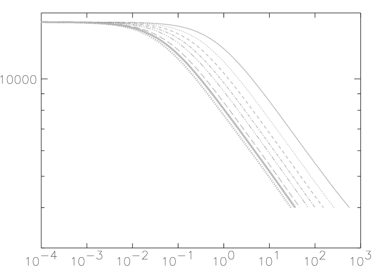
Figure 16: Expansion velocity of each layer as a function of $\tau_{std}$ for the SN 1999em model. The colors and line-styles are the same as in Figure 13.

Figure 16 of Dessart & Hillier (2008) compares the observed spectra of SN 1999em for 48.7 days since explosion and the spectra calculated from both time dependent and independent models for the rate equations. One may notice a significant mismatch between the time dependent model and observed spectra in certain regions where the time independent models matches better. Around 4000 Å, the Fe I, Fe II lines are not reproduced well (Pastorello et al., 2004), similarly the C I and Ca II line strengths around 8600 Å are underestimated using the time dependent model and the line strengths are better reproduced by the time independent model. Dessart & Hillier (2008) find that time dependence is better for later epochs, from their work on SN 1999em and SN 1999br, about 30 days after explosion.

4 Description of PHOENIX

PHOENIX is a model atmosphere computer code that has been developed by Hauschildt, Baron and collaborators over the last two decades. Due to the coupling between the level populations and the radiation field, the radiation transport equation must be solved simultaneously with the rate equations. PHOENIX includes a large number of NLTE and LTE background spectral lines and solves the radiative transfer equation with a full characteristics piecewise parabolic method (Olson & Kunasz, 1987; Hauschildt, 1992) and without simple approximations like the Sobolev approximation (Mihalas, 1970). Hauschildt & Baron (1999) describe the numerical algorithms used in PHOENIX to solve the radiation transport equations, the non-LTE rate equations and parallelization of the code. PHOENIX uses the total bolometric luminosity in the observer’s frame, the density structure, and element abundances as input parameters. The equation of radiative transfer in spherical geometry, the rate equations, and the condition of radiative equilibrium are then solved. This process is repeated until the radiation field and the matter have converged to radiative equilibrium in the Lagrangian frame. In our model calculations we have not taken into account the ionization by non thermal electrons. Also time dependence was incorporated only in the rate equations. The inclusion of time dependence in the thermal equilibrium equation is implicit. Since the time dependent rate equations affect the opacities, the solution of the radiative transfer equation is affected as well. The explicit implementation of time dependence in the radiative transfer equation is beyond the scope of this work. Our goal was to specifically examine the effects of time dependence on the hydrogen Balmer lines and therefore only hydrogen is treated in NLTE. This both speeds up the calculations significantly and isolates the effects of time dependence on hydrogen.

5 Recombination Time Calculations

Our main motivation is to explore the recombination time in a SN II atmosphere. In order to obtain the correct electron densities and level populations it is essential to make sure that the rate equations are correct even if the recombination time is actually longer or comparable to the age of the supernova. We incorporated the time dependent term in the rate equations and in our results we describe this as the time dependent case. We have performed calculations assuming both the steady-state, time-independent, (TI), approximation as well as the full time-dependent, (TD), rate equations. In most of our models we used a hydrogen model atom consisting of 31 levels. To save computing time and limit the time-dependent effects to the Balmer lines, we treated all other elements in LTE for this work. We started with a known density profile typical of a SN II with mass similar to the progenitor mass of SN 1987A ($\sim 14.7M_{\odot}$) and luminosity ($1.015\times$ $10^{43}$ ergs) . We built a radial velocity grid with 128 layers. The location of the radial points was found from the assumption of homology, $r=vt$. PHOENIX then solves the radiative transfer equation and the rate equations simultaneously. This yields the temperature, radiation field, and other physical parameters such as pressure, optical depth, and electron density for each radial grid or layer. We choose the best model by tuning only the input luminosity and the input density profile by comparing the match between the synthetic and the observed spectra of SN 1987A.

We began with a time-independent model at Day 2 and generated snapshots for both the time dependent and independent cases up to Day 20 with intervals of 2 days. It is important for the time-dependent case to have the correct level populations at the previous time and consequently it was better to choose a smaller time interval (two days) to generate snapshots of the physical profile of the supernova. Our analysis was done on a Lagrangian velocity grid. Right after the explosion, the optical depth is very high in the innermost layers that are expanding with low velocity. At very high optical depth, radiative diffusion is an excellent approximation. Thus at high optical depths we replace the innermost ejecta with an opaque core and the luminosity is given by the expression for radiative diffusion at this boundary. Our initial grid has has a velocity of $\sim 3000$ km s^-1 and we gradually add deeper layers until at our final epoch of 20 days, the innermost layer has a velocity of around $\sim 1000$ km s^-1. To add new layers in the inner core we merged the outer low density, high velocity layers keeping the total number of layers constant. This way we preserved the grid size but also made sure that we have the physically relevant velocity range at all epochs of evolution.

In order to recover the results of UC05 in a simple hydrogen model atom case and also to understand the difference between the simple and multi-level model atom framework we repeated our calculations for a 4-level hydrogen atom model case with solar compositions. In order to have the correct physical conditions, we held the structure of the atmosphere (temperature and density) fixed from what we had obtained with the time-dependent multi-level hydrogen atom case for that epoch. We then solved for the time-dependent level populations and the associated radiation field.

6 Results

Our computations consist of three different systems at each epoch. They are the case when we have a 4-level ($n=2$) hydrogen model atom in NLTE (in absence of any other metals) and time-dependent rate equations. We refer to this model as Case 1. Cases 2 and 3 are full calculations with 31-level hydrogen model atoms, solar compositions, and time-dependent and time-independent rate equations, respectively.

We measure the optical depth using the value $\tau_{\mathrm{std}}$ which is the optical depth in the continuum at 5000 Å.

6.1 Ionization Fraction and Electron Density Profile

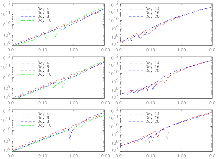
Figure 1: Comparison between the free electron densities at different systems. The upper panel has 4-level hydrogen atom case. The middle panel has the multilevel time dependent case. The bottom panel has the multilevel time independent case.

The two most important physical parameters for the recombination time are the ionization fraction, $f_{H}$, and the free electron density, $n_{e}$. In Figure 1 we present the electron density for the three different cases.

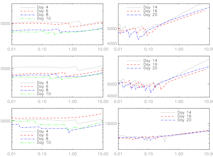
Figure 2: Comparison between electron temperatures at different systems. The upper panel has 4-level hydrogen atom case. The middle panel has the multilevel time dependent case. The bottom panel has the multilevel time independent case.

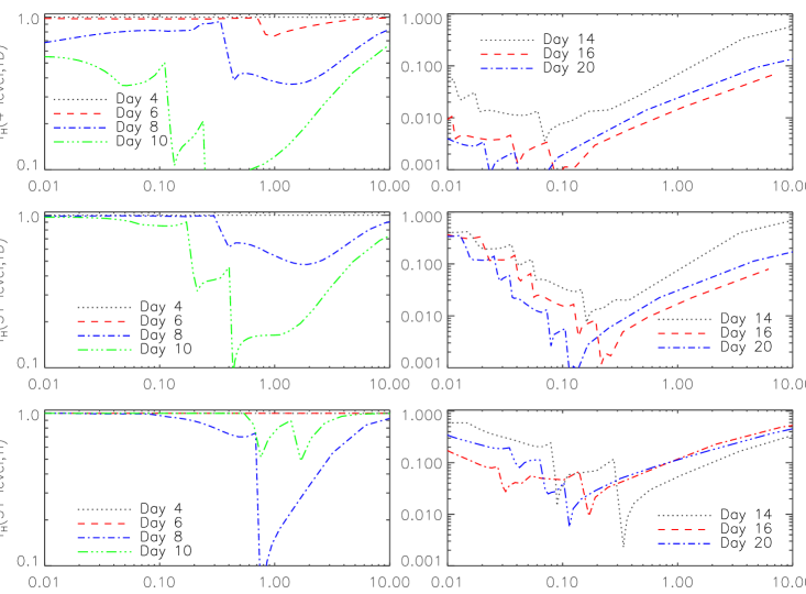
Figure 3: Comparison between ionization fractions at different systems. The upper panel has 4-level hydrogen atom case. The middle panel has the multilevel time dependent case. The bottom panel has the multilevel time independent case.

The upper panel shows the free electron density for Case 1 (where only hydrogen is present with $n=2$ and rate equations are time dependent) over different epochs. Days 2–6 show a steady rise in the free electron density in the system as the optical depth becomes higher. The electron density declines at later epochs due to cooling and geometric dilution. These trends of high electron density at very early epochs and lower electron density at the later epochs are expected from the fact that the temperature is high at early times. At later epochs, the electron density at a given optical depth falls off due to the expansion and declining temperature. At epochs 4–6 d, the hydrogen in the system is almost completely ionized and the free electron density is the highest at this epoch. In the right plot of the top panel of Figure 1 we display the electron density for the epochs 14–20 d. At these epochs, hydrogen ionization is lower and recombination of hydrogen begins. This is evident from the corresponding temperature structure. Figure 2 displays the electron temperature of the system, which controls the free electron density and the level of ionization. The top left panel displays the temperatures for early epochs ($T\sim 8000-10000$ K for epochs $<8$ d). In the top right panel the temperature drops to around 5000 K and this is where the transition from the fully ionized to the partially ionized regime occurs. The recombination regime begins roughly at day 8. Between optical depths $\tau_{\mathrm{std}}=0.01-0.1$, the temperature is around 5000 K for epochs later than about 8 d since explosion, thus recombination starts to take place, reducing the free electron density. For optical depths higher than $\tau_{\mathrm{std}}=0.1$, the electron temperature is still high enough (even at later epochs) to maintain a high level of ionization. Using the values of the free electron density and the temperature structure it is easy to understand the ionization fraction for hydrogen in the system which is displayed in Figure 3. The optical depth is indicated using the value $\tau_{\mathrm{std}}$ which is the optical depth in the continuum at 5000 Å. Beginning at 6 d for Case 1, recombination starts to take place at optical depths $\tau_{\mathrm{std}}=0.01-0.1$ causing a bumpy profile for the ionization fraction.

For Case 2, (time-dependent rate equations and multi-level hydrogen with 31 bound levels) results are displayed in the middle panel of our figures. We again refer to the middle panel of the Figures 1–3. The basic nature of the temperature structure, free electron density, and the ionization fraction are very similar to Case 1. The main difference in this case is that for the later epochs, the electron temperature is around 5000 K for optical depths $\tau_{\mathrm{std}}=0.01-0.3$. Thus, the recombination front moves deeper into the expanding ejecta for the multilevel case with metals. This may be a cumulative effect due to the metals and the multiple bound levels. The metals tend to suppress the ionization of hydrogen at higher optical depths, hence we would expect the ionization front for hydrogen to move deeper into the object. The multiple bound levels enhance the recombination at any optical depth. The ionization fraction for hydrogen follows the free electron density and the temperature profile by producing a bumpy profile between for $\tau_{\mathrm{std}}=0.01-0.3$.

For Case 3, where the rate equations are time-independent with the 31-level hydrogen model atom, results are shown in the bottom panel of our plots. In this case the recombination front moves deeper inside compared to Cases 1 and 2. Thus, the electron temperatures of about 5000 K are reached at optical depths $\tau_{\mathrm{std}}>1.0$ for later epochs.

To summarize our results on the ionization fraction: 1) In all three cases we observed that the results from the free electron density, electron temperature and ionization fraction are consistent with each other. 2) As the supernova expands, the recombination front moves deeper inside. The span of the recombination front is different in all three cases, being largest in Case 3. Overall, the free electron densities are similar in all three cases. 3) In the recombining regime, the electron density drops, causing a drop in the ionization fraction as well. 4) All three cases (31 level time dependent, 31 level time independent and 4 level time dependent) have visibly different ionization fraction profiles, but the difference decreases between Cases 2 and 3 (31 level hydrogen model). In other words Case 1 has the ionization profile that is different from Case 2 and Case 3. The ionization fraction in these models after 10 days is higher than that in the 4 level hydrogen atom time dependent model (Case 1). 5)In the recombination regime, there are glitches at the recombination front which probably arise from the imperfect spatial resolution of the ionization front. It is clear from the figures that the glitches do not affect the overall qualitative results.

6.2 Spectral comparison

Spectra are important as they are the only observable. In our discussion we emphasize the $H_{\alpha}$ profile of the spectra. In Figure 5 we present the comparison between the $H_{\alpha}$ line profile of the spectra for the Cases 2 and 3. In this plot we have days 4, 6, and 8. We used dotted lines for Case 3 and solid lines for Case 2 in all our line profile and spectral comparison plots. The very early $H_{\alpha}$ profiles do not show any differences between Cases 2 and 3. From Day 6 onwards we notice that the line profile gets wider for Case 2 — the time dependent case. Figure 7 shows a spectral comparison between Cases 2 and 3. Overall, the spectral features for the Case 2 are somewhat broader (especially between $4000-6500$ Å).

We plot the $H_{\alpha}$ profile for days 10, 14, 16, and 20 for Cases 2 and 3 in Figure 6. We see a similar broadening in the profile for Case 2 except at day 16. This broadening becomes more obvious if one looks at the spectral plot (Figure 8). The spectra seem to have somewhat broader features for Case 2, especially in the regime $\lambda<4500$ Å and $\lambda>8000$ Å. We emphasize that these spectral profiles for SN 1987A were generated by independently tuning their luminosity to obtain the best fit to the observed spectra. To summarize we find that the spectral features become somewhat broader with time dependent treatment of the rate equations, but the effect is smaller than that found by Dessart & Hillier (2008).

Figure 9 shows a comparison of the model spectra with observations for SN 1987A at days 4 and 6. There is a noticeable improvement in the $H_{\alpha}$ profile for the time dependent case versus the time-independent case, although some of the effect is due to variations in the luminosity which is a parameter in our models. Thus, time dependent effects can be important for the early epoch $H_{\alpha}$ profiles.

6.3 Results on the recombination time

The recombination time is a crucial quantity. The motivation for this paper was to study if the apparent importance of time dependence could be verified from the numerical estimate of the effective recombination time. It is important to check if the effective recombination time is essentially comparable to the age of the supernova. Since our spectra were generated by independently tuning the luminosity, it is important to investigate the recombination time scale to be able to conclude if the time dependence in the rate equations is indeed important. As noted above, the semi-analytic result is for a two-level atom and the effects of both non-resonant de-excitations and a reduction in the escape probability due to more channels could alter the numerical values compared to the simpler analysis. Figure 4 shows the recombination time for Cases 1 and 2.

Case 1, shown in the upper panel of Figure 4, the recombination time (referred as $\tau_{H(4)}$) follows an inverted profile compared to the ionization fraction (see Figure 3). This is consistent with the fact that the low ionization fraction will reduce recombination, resulting in a longer recombination time. Similar to the profiles for the ionization fraction and the electron density, the recombination time also gives a bumpy structure in the recombining region. In Case 1, for epochs $>6$ d the recombination time is around $10^{6}-10^{7}$ for $\tau_{\mathrm{std}}=0.01-0.1$. Below the recombining regime, the recombination time is lower. This is due to the increasing density. At lower $\tau_{\mathrm{std}}$, the recombination time increases because the electron density declines.

The bottom panel of Figure 4 shows the recombination time for Case 2. The numerical value of the recombination time, $\tau_{H(31)}$, is highest for the earliest epochs. This is because there is barely any recombination since the temperature is $T>10^{4}$ K (see Figure 2). After the initial expansion, the electrons start to recombine. At the ionization front, due to the falling electron density, the recombination time increases at later epochs. Although outside of the ionization front the recombination time decreases with the expansion of the supernova. This is the case both for $\tau_{H(4)}$ and $\tau_{H(31)}$ except that this effect is more evident at later epochs in the multi-level case (bottom panel of Figure 4). To summarize: 1) $\tau_{H(31)}$ and $\tau_{H(4)}$ follow the profile expected from their respective free electron density and temperature profiles and almost follow an inverted profile compared to the ionization fraction profile. In other words, the recombination time is found to be proportional to the free electron density and temperature and inversely proportional to the ionization fraction.

2) The recombination time is higher for low optical depths. There is a break in the monotonic decline in the recombination time (as it moves toward higher optical depth) in the recombining regime. There is a rise in the recombination time in this regime. For optical depths $\tau_{\mathrm{std}}>1.0$, both $\tau_{H(31)}$ and $\tau_{H(4)}$ decrease monotonically due to the increase in the free electron density.

3) As the supernova expands, the recombination time at a given optical depth decreases at almost all optical depths (Figure 4).

4) Figure 12 compares the time-dependent multi-level hydrogen atom and the classical recombination time, $\tau_{anal}$. In the optically thin regime ($\tau_{std}<0.10$) $\tau_{H(31)}$ is close to $\tau_{anal}$. Only right at the ionization front doe the ratio deviate significantly from unity and $\tau_{H(31)}$ is larger than $\tau_{anal}$.

7 SN 1999em

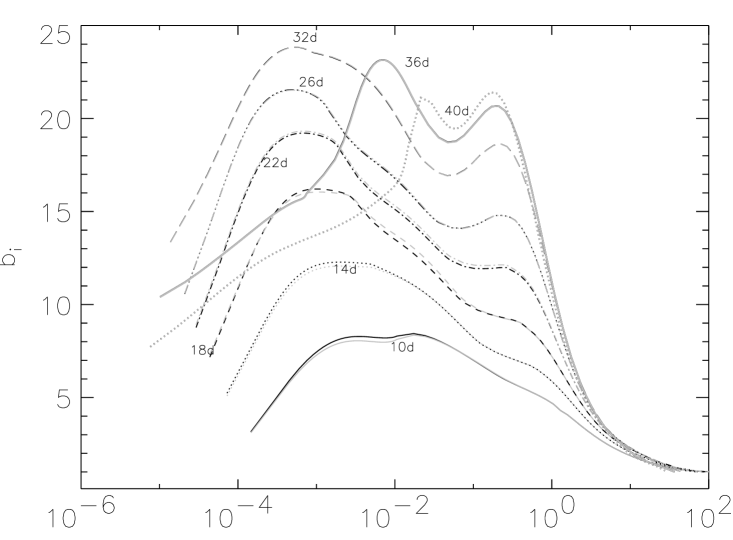
Figure 14: Departure coefficient, $b_{2}$, as a function of $\tau_{std}$ for the $n=2$ state of hydrogen. The colors and line-styles are the same as in Figure 13.

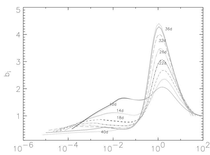
Figure 15: Departure coefficient, $b_{3}$, as a function of $\tau_{std}$ for the $n=3$ state of hydrogen. The colors and line-styles are the same as in Figure 13.

SN1987A is one of the best observed astronomical objects. It is also a peculiar Type II supernova. It has two maxima in its light curve and it also has very steep rise to its maximum. On the other hand SN 1999em has steady rise to the maximum and a well-defined plateau. Thus, we also studied the effects of time-dependence in SN 1999em. We began with the day 7 spectrum and marched forward in time until around day 40 (since explosion). We again considered a 31 level hydrogen atom and treated only hydrogen in NLTE. The departure coefficients (referred as $b_{i}$) are the ratio of the real level population density to the expected LTE level population density (Menzel & Cillié, 1937; Mihalas, 1978). Figures 13–15 display the departure coefficients for the levels $n=1$ (ground state), $n=2$, and $n=3$. It is evident from our plots that time dependence is important at early times although the effect is very small. This effect diminishes with time. Also the effect is only relevant in the recombining regime. The explanation of this transient phenomenon is easier to understand in the Lagrangian frame. In a given mass element at very early times if the temperature is much higher than 5000 K, the hydrogen is nearly completely ionized and the $\frac{d}{dt}$ term is very small. At very late times when the temperature falls much below 5000 K, the hydrogen is mostly neutral and the $\frac{d}{dt}$ term is also small. Thus, the $\frac{d}{dt}$ term is important in the recombination regime. The effect decreases with time. Our results agree with those of UC05. The calculations are performed on a Lagrangian grid, however, the results are best presented on the $\tau_{std}$ grid. As an aid to interpreting these figures, Figure 16 shows the profile of velocity vs $\tau_{std}$. We find that the change in the departure coefficients for the ground state is up to 12%. For the first and second excited states the change in the departure coefficients is up to 4% and 2% respectively. The change was found to be maximum at day 10. In order to test the sensitivity of our results to the timestep we compared our results for SN 1999em for the case where we use a 4 day interval to that where we use 1 day interval in the time dependent rate equation for hydrogen. We find in the 14 day spectra, the change in the departure coefficients (derived from two different timesteps) is within 3% (for the ground state) in the line forming region. This effect becomes even smaller at later times.

8 Discussion and Conclusions

We have studied the importance of time-dependence in the rate equations in a type II supernova atmosphere due to the increase in the recombination time. We also explored the effects of having many angular momentum sub-states. In our description we use $\tau_{H(4)}$ and $\tau_{H(31)}$ as the recombination time for a 4-level hydrogen atom model and 31-level hydrogen atom model respectively.

1) UC05 proposed that $\tau_{H(4)}$ is of the order of $10^{7}$ s at $T\sim 5000$ K and $n_{e}=10^{8}$ cm^-3. For epochs later than 6 days, we calculated $\tau_{H(4)}$ at similar electron density and temperature to be around $10^{7}$ s ($\tau_{\mathrm{std}}\sim 0.02$). Thus, we recover the recombination time scale predicted by UC05 for the 4-level hydrogen case. An important difference between our results and those of UC05 is that we find the electron densities and temperatures which they used as photospheric conditions to occur at $\tau_{\mathrm{std}}\sim 0.02$ and not near $\tau_{\mathrm{std}}=1.0$. Around $\tau_{\mathrm{std}}=1.0$, the free electron density even for Case 1 is much higher and hence the recombination time is much smaller. This optical depth mismatch is due to the fact that we are looking at the continuum optical depth and not the line optical depth. The ratio of the Balmer line opacity to the continuum opacity is $\sim 10^{3}$ in the recombining region.

We also compare the classical recombination time (calculated using $1/\alpha n_{e}$) with our calculated $\tau_{H(4)}$ generated from the solution of the radiative transfer equation. We refer to the approximate classical recombination time as $\tau_{anal}$. This allows us to determine the factor $w_{21}$ (UC05). Figure 11 displays the ratio $\tau_{anal}/\tau_{H(4)}$, a direct measure of $w_{21}$ described by UC05.

In Figure 10, we display the ratio of the recombination time for Case 2 to the recombination time from a simple hydrogen atom (Case 1) at the same epoch and at the same optical depth.

1) For all epochs, $\tau_{H(31)}$ is smaller than $\tau_{H(4)}$ at almost all optical depths. For higher optical depths, the ratio increases and approaches unity. because the ionization fraction for hydrogen and $\tau_{H(31)}$ becomes independent of the number of bound levels. At this point the system is almost in LTE and the number of free electrons depends only on the temperature. 2) Figure 11 shows that the simple hydrogen atom model (4-level) overestimates the recombination time by a factor of 100 or more at all almost all epochs and optical depths. 3) Figure 12 shows that the recombination time recovered from a multi-level hydrogen atom compares with the standard value ($\tau_{anal}$) for $\tau_{std}<1.0$. At the ionization front $\tau_{H(31)}$ differs significantly from $\tau_{anal}$. 4) Based on our work on SN 1999em, we find that the transient nature of the level population of hydrogen is not a crucial factor on the plateau, but it is important in the active recombining regime. This effect could be important for early features in the spectra but the steady state approximation should be valid in the plateau phase. 5) In the early early spectra of SN 1987A we find that $H_{\alpha}$ is better fit using the time-dependent formulation. 6) The recombination time jumps above the underlying trend only at the ionization front. This is just caused by the sudden reduction of the electron density driving the the recombination time higher in the ionization front.

It is very difficult to decouple the effects of time dependent rate equations in a radiative transfer framework and the effects of multi-level model atoms by only looking at spectra. The Balmer profile of the spectra of SN 1987A at early times (Figure 9) and the level populations from our results on SN 1999em (Figure 13 – 15), indicate the effects of the time dependent rate equations at early times. The increased recombination time (Figure 4) at early times for SN 1987A also supports the importance of time-dependent rate equations. Therefore we conclude that time dependence is more important at early times than later times. The effect of multi-level atoms can be seen in Figure 4 which clearly shows than even at later times $\tau_{H(4)}$ is much higher than $\tau_{H(31)}$. Therefore conclusions using only a 4-level model may overestimate the importance of time dependence. Of course, including time-dependence is not terribly costly numerically and thus it can be included when a time sequence is calculated.

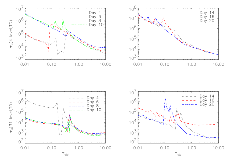
Figure 4: Comparison between recombination times at different systems. The upper panel has 4-level hydrogen atom case. The middle panel has the multilevel time dependent case. The bottom panel has the multilevel time independent case.

Figure 5: Comparison of the line profiles of $H_{\alpha}$ for Days 4, 6, 8 in the time dependent and time independent cases for a model that is appropriate to SN 1987A. The luminosity in each case has been tuned to fit the observations.

Figure 6: Comparison of the line profile of $H_{\alpha}$ for Days 10, 14, 16, 20 in the time dependent and time independent cases for a model that is appropriate to SN 1987A. The luminosity has been tuned to fit the observations in each case.

Figure 7: Comparison of the spectra for Days 4, 6, 8 in the time dependent and time independent cases for a model that is appropriate to SN 1987A. The luminosity in each case has been tuned to fit the observations. The differences in the day 6 UV spectra are primarily due to variations in the opacity due to the exponential dependence of the Fe II populations on the temperature and not to time dependence in the hydrogen rate equations.

Figure 8: Comparison of the spectra for Days 10, 14, 16, 20 in the time dependent and time independent cases for a model that is appropriate to SN 1987A. The luminosity in each case has been tuned to fit the observations.

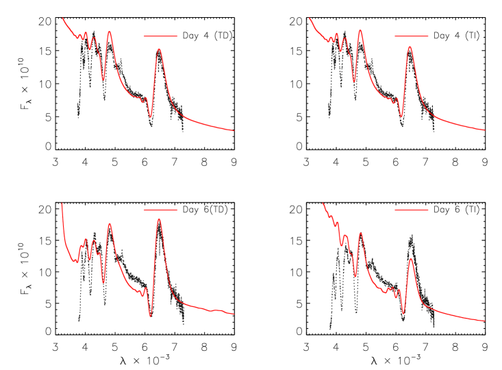
Figure 9: Comparison of the spectra day 4 and 6 with time dependent and time independent cases with observed spectra of SN 1987A. The luminosity in each case has been tuned to fit the observations. The $H_{\alpha}$ profile is improved in the time dependent case.

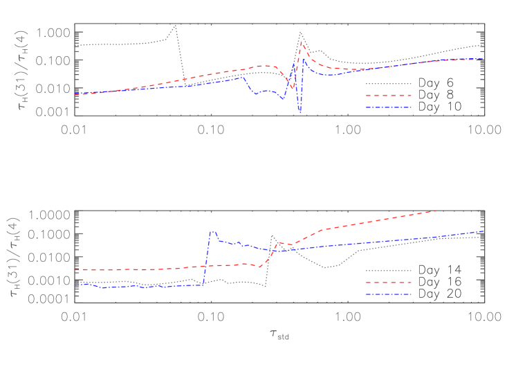
Figure 10: Ratio of recombination times for the time dependent multilevel hydrogen atom case and the 4-level hydrogen atom model calculated at different days. The upper panel shows the earlier epochs and the lower panel the later epochs.

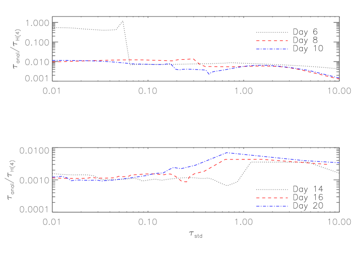
Figure 11: Ratio of recombination times for the analytical calculation and the 4-level hydrogen atom model calculated at different epochs. The upper panel shows the earlier epochs and the lower panel the later epochs.

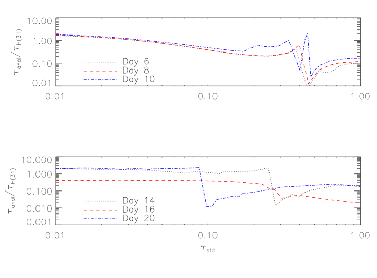
Figure 12: Ratio of recombination times for the analytical calculation and the 31-level hydrogen atom model calculated at different epochs. The upper panel shows the earlier epochs and the lower panel the later epochs.

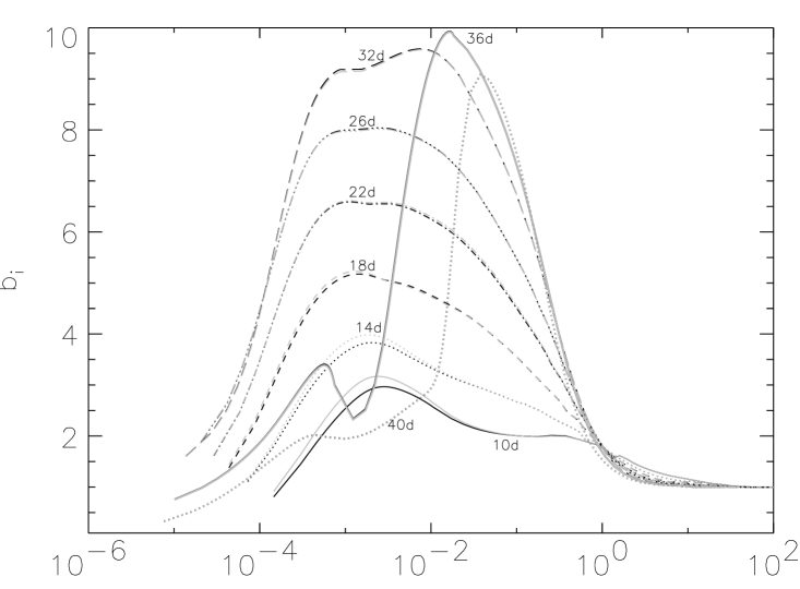
Figure 13: Departure coefficient, $b_{1}$, as a function of $\tau_{std}$ for the ground state of hydrogen. The black line is for the time dependent case and grey line is the time independent case for each day.

References

- Arnett et al. (1989) Arnett W. D., Bahcall J., Kirshner R. P., Woosley S. E., 1989, Ann. Rev. Astr. Ap., 27, 629
- Carlsson et al. (1992) Carlsson M., Rutten R., Shchukina N., 1992, A&A, 253, 567
- Chandrasekhar (1934) Chandrasekhar S., 1934, MNRAS, 94, 444
- Danziger et al. (1988) Danziger I. J., Bouchet P., Fosbury R. A. E., Gouiffes C., Lucy L. B., 1988, in M. Kafatos & A. G. Michalitsianos ed., Supernova 1987A in the Large Magellanic Cloud SN 1987A - Observational results obtained at ESO. pp 37–50
- Dessart & Hillier (2005) Dessart L., Hillier D. J., 2005, A&A, 439, 671
- Dessart & Hillier (2008) Dessart L., Hillier D. J., 2008, MNRAS, 383, 57
- Hanuschik & Dachs (1988) Hanuschik R. W., Dachs J., 1988, Astronomy and Astrophysics, 205, 135
- Hauschildt (1992) Hauschildt P. H., 1992, JQSRT, 47, 433
- Hauschildt & Baron (1999) Hauschildt P. H., Baron E., 1999, J. Comp. Applied Math., 109, 41
- Hillier & Miller (1998) Hillier D. J., Miller D. L., 1998, ApJ, 496, 407
- Höflich (1988) Höflich P., 1988, Proceedings of the Astronomical Society of Australia, 7, 434
- Höflich (2003) Höflich P., 2003, in ASP Conf. Ser. 288: Stellar Atmosphere Modeling ALI in Rapidly Expanding Envelopes. p. 185
- Hummer & Storey (1987) Hummer D. G., Storey P. J., 1987, MNRAS, 224, 801
- Mazzali et al. (1992) Mazzali P. A., Lucy L. B., Butler K., 1992, A&A, 258, 399
- Menzel & Cillié (1937) Menzel D. H., Cillié G. G., 1937, ApJ, 85, 88
- Mihalas (1970) Mihalas D., 1970, Stellar atmospheres. Series of Books in Astronomy and Astrophysics, San Francisco: Freeman, —c1970
- Mihalas (1978) Mihalas D., 1978, Stellar Atmospheres. W. H. Freeman, New York
- Olson & Kunasz (1987) Olson G. L., Kunasz P. B., 1987, JQSRT, 38, 325
- Osterbrock (1989) Osterbrock D., 1989, Astrophysics of Gaseous Nebulae and Active Galactic Nuclei. University Science Books, Mill Valley, CA
- Pastorello et al. (2004) Pastorello A., Zampieri L., Turatto M., Cappellaro E., Meikle W. P. S., Benetti S., Branch D., Baron E., Patat F., Armstrong M., Altavilla G., Salvo M., Riello M., 2004, MNRAS, 347, 74
- Peebles (1968) Peebles P. J. E., 1968, ApJ, 153, 1
- Perlmutter et al. (1999) Perlmutter S., et al., 1999, ApJ, 517, 565
- Riess et al. (1998) Riess A., et al., 1998, AJ, 116, 1009
- Saio et al. (1988) Saio H., Nomoto K., Kato M., 1988, ApJ, 331, 388
- Schmutz et al. (1990) Schmutz W., Abbott D. C., Russell R. S., Hamann W.-R., Wessolowski U., 1990, ApJ, 355, 255
- Utrobin & Chugai (2005) Utrobin V. P., Chugai N. N., 2005, Astronomy and Astrophysics, 441, 271
- Williams (1987a) Williams R. E., 1987a, ApJ, 320, L117
- Williams (1987b) Williams R. E., 1987b, in Nomoto K., ed., Atmospheric Diagnostics of Stellar Evolution Supernova 1987 A in the Large Magellanic Cloud - Possible s-process enhancements in the progenitor. Springer, Berlin, p. 118
- Zeldovich et al. (1969) Zeldovich Y. B., Kurt V. G., Syunyaev R. A., 1969, Soviet Journal of Experimental and Theoretical Physics, 28, 146