Non-collinear spin-spiral phase for the uniform electron gas within
Reduced-Density-Matrix-Functional Theory

Abstract

The non-collinear spin-spiral density wave of the uniform electron gas is studied in the framework of Reduced-Density-Matrix-Functional Theory. For the Hartree-Fock approximation, which can be obtained as a limiting case of Reduced-Density-Matrix-Functional Theory, Overhauser showed a long time ago that the paramagnetic state of the electron gas is unstable with respect to the formation of charge or spin density waves. Here we not only present a detailed numerical investigation of the spin-spiral density wave in the Hartree-Fock approximation but also investigate the effects of correlations on the spin-spiral density wave instability by means of a recently proposed density-matrix functional.

I Introduction

For many decades, the uniform electron gas has served as the model for the description of many-particle systems Giuliani and Vignale (2005a). However, the determination of its ground state, without any symmetry assumptions, still remains a challenge. Specific symmetries for the fully correlated uniform electron gas have been investigated using Monte Carlo methods Ceperley and Alder (1980); Ortiz et al. (1999). These studies focus mostly on broken spatial symmetry, i.e. , Wigner crystallization, or broken global spin symmetry.

For the electron gas with constant electron density and uniform spin-polarization, the ground-state energy is analytically accessible in the Hartree-Fock approximation. Overhauser showed in his seminal work Overhauser (1960, 1962) that within the Hartree-Fock approximation the aforementioned homogeneous ground state exhibits an instability w.r.t. the formation of charge and spin density waves. Wigner crystallization within Hartree-Fock has been investigated in Ref. Trail et al., 2003. Only recently the combined local spatial- and spin-symmetry breaking of the Hartree-Fock ground state has been studied using a Monte Carlo method which optimizes the ground-state energy in the space of single Slater-determinants Zhang and Ceperley (2008). However, this study still remains in the regime of collinear spin polarization.

In the present work we investigate the case of local spin symmetry breaking, specifically a non-collinear spin-spiral symmetry. We employ Reduced-Density-Matrix-Functional Theory both in the limiting case of the Hartree-Fock approximation as well as for the correlated electron gas using the recently proposed density-matrix-power functional Sharma et al. (2008); Lathiotakis et al. (2009).

II Theoretical framework

II.1 Reduced-Density-Matrix-Functional Theory

The basic variable in Reduced-Density-Matrix-Functional Theory (RDMFT) is the one-body-reduced density matrix (1-RDM) defined by

$$\gamma_{\sigma\sigma^{\prime}}\!\left(\boldsymbol{r};\boldsymbol{r}^{\prime}\right)\equiv\operatorname{Tr}_{N}\!\left\{\hat{D}\hat{\psi}^{\dagger}_{\sigma^{\prime}}\!\left(\boldsymbol{r}^{\prime}\right)\hat{\psi}_{\sigma}\!\left(\boldsymbol{r}\right)\right\}$$ (1)

where $\hat{D}$ is the zero-temperature statistical operator of an ensemble of $N$-electron states

$$\hat{D}\equiv\sum_{i}\omega_{i}^{2}\left|\Psi^{N}_{i}\right\rangle\left\langle\Psi^{N}_{i}\right|\;\;\mbox{with}\;\;\sum_{i}\omega_{i}^{2}=1,$$ (2)

where ${\hat{\psi}^{\dagger}_{\sigma}\!\left(\boldsymbol{r}\right)}$ and ${\hat{\psi}_{\sigma}\!\left(\boldsymbol{r}\right)}$ are fermionic creation and annihilation operators, respectively. The 1-RDM is a Hermitian operator in the single-particle Hilbert space and can be represented by its spectral decomposition

$$\gamma\!\left(\boldsymbol{r};\boldsymbol{r}^{\prime}\right)=\sum_{i}n_{i}\Phi_{i}\!\left(\boldsymbol{r}\right)\Phi^{\dagger}_{i}\!\left(\boldsymbol{r}^{\prime}\right),$$ (3)

where the eigenvalues $n_{i}$ are called occupation numbers (ON) and the corresponding single-particle Pauli-spinor eigenstates $\Phi_{i}(\boldsymbol{r})=\left(\varphi_{i\uparrow}\!\left(\boldsymbol{r}\right),\varphi_{i\downarrow}\!\left(\boldsymbol{r}\right)\right)^{T}$ are referred to as natural orbitals (NO). It was shown by Gilbert Gilbert (1975) that the $N$-particle ground state is a unique functional of the ground state 1-RDM, i.e. , $\left|\Psi^{N}_{0}\right\rangle=\left|\Psi^{N}_{0}\!\left[\gamma^{\mathrm{gs}}\right]\right\rangle$ . Therefore the ground state energy for a system of $N$ interacting electrons moving in an arbitrary but fixed (possibly non-local) external potential $\hat{V}$ is also a functional of the 1-RDM:

$$E_{\mathrm{V}}\!\left[\gamma^{\mathrm{gs}}\right]=\left\langle\Psi^{N}_{0}\!\left[\gamma^{\mathrm{gs}}\right]\right|\hat{\mathcal{H}}_{V}\left|\Psi^{N}_{0}\!\left[\gamma^{\mathrm{gs}}\right]\right\rangle\;,$$ (4)

where ${\hat{\mathcal{H}}_{V}=\hat{T}+\hat{V}+\hat{W}+E_{\mathrm{ion}}}$ is a generic interacting many-body Hamiltonian with kinetic energy $\hat{T}$, external potential $\hat{V}$, electron-electron interaction $\hat{W}$, and a constant energy contribution $E_{\mathrm{ion}}$ from the degrees of freedom that are not treated quantum mechanically.

The ground-state-energy functional can be decomposed into the following components

$$E_{\mathrm{V}}\!\left[\gamma\right]=T\!\left[\gamma\right]+V\!\left[\gamma\right]+W\!\left[\gamma\right]+E_{\mathrm{ion}},$$ (5)

with the kinetic energy (atomic units are used throughout the paper, and the superscript “gs” is omitted for brevity)

$$T\!\left[\gamma\right]=\sum_{\sigma}\int\!\!\mathrm{d}^{3}r\lim_{\boldsymbol{r}^{\prime}\to\boldsymbol{r}}\frac{1}{2}\nabla^{\prime}\nabla\gamma_{\sigma\sigma}\!\left(\boldsymbol{r};\boldsymbol{r}^{\prime}\right),$$ (6)

and the energy contribution due to the external potential

$$V\!\left[\gamma\right]=\sum_{\sigma}\int\!\!\mathrm{d}^{3}rV\!\left(\boldsymbol{r}\right)\gamma_{\sigma\sigma}\!\left(\boldsymbol{r};\boldsymbol{r}\right).$$ (7)

Here we are assuming a local, spin independent external potential. The Hohenberg-Kohn theorem of Density-Functional Theory (DFT) proves a one-to-one mapping between the ground-state density and the N-particle ground state, considering only local external potentials. However, in RDMFT the Gilbert theorem ensures a one-to-one correspondence between the ground-state 1-RDM and the N-particle ground state by considering the broader class of non-local external potentials. This also implies the one-to-one mapping between a local potential and the ground-state 1-RDM. Note that in contrast to usual Kohn-Sham DFT all single-particle contributions to the ground state energy $E_{\mathrm{V}}$ are explicitly given in terms of the ground state 1-RDM. However, the interaction energy

$$W\!\left[\gamma\right]=\sum_{\sigma_{1}\sigma_{2}}\iint\!\!\mathrm{d}^{3}r_{1}\mathrm{d}^{3}r_{2}\frac{P^{\mathrm{gs}}_{\sigma_{1}\sigma_{2}}\!\left[\gamma\right]\!\left(\boldsymbol{r}_{1},\boldsymbol{r}_{2}\right)}{\left|\boldsymbol{r}_{1}-\boldsymbol{r}_{2}\right|},$$ (8)

is only known explicitly in terms of the ground-state pair density

$$P^{\mathrm{gs}}_{\sigma_{1}\sigma_{2}}\!\left[\gamma\right]\!\left(\boldsymbol{r}_{1},\boldsymbol{r}_{2}\right)\equiv$$

$$\left\langle\Psi^{N}_{0}\!\left[\gamma\right]\right|\hat{\psi}^{\dagger}_{\sigma_{1}}\!\left(\boldsymbol{r}_{1}\right)\hat{\psi}^{\dagger}_{\sigma_{2}}\!\left(\boldsymbol{r}_{2}\right)\hat{\psi}_{\sigma_{2}}\!\left(\boldsymbol{r}_{2}\right)\hat{\psi}_{\sigma_{1}}\!\left(\boldsymbol{r}_{1}\right)\left|\Psi^{N}_{0}\!\left[\gamma\right]\right\rangle\;.$$ (9)

The basic idea of RDMFT is to extend the domain of the ground-state-energy functional in Eq. (4) to all ensemble-$N$-representable 1-RDMs [as defined in Eq. (1)] and then employ the variational principle in order to find the ground-state 1-RDM as well as the ground-state energy corresponding to a fixed external potential $V$. The necessary and sufficient conditions for a 1-RDM to be ensemble-$N$-representable are Coleman (1963):

$$\sum_{i}n_{i}=N\;\;\mbox{and}\;\;0\leq n_{i}\leq 1,$$ (10a)

$$\sum_{\sigma}\int\!\!\mathrm{d}^{3}r\varphi^{\star}_{i\sigma}\!\left(\boldsymbol{r}\right)\varphi_{j\sigma}\!\left(\boldsymbol{r}\right)=\delta_{ij}.$$ (10b)

In order to apply RDMFT in practice we need to approximate the functional dependence of the pair density on the 1-RDM. Since we want to study the spin-spiral density wave (SSDW) instability in the uncorrelated (Hartree-Fock, HF) and the correlated regime, we focus on the so-called density-matrix-power functional introduced in Ref. Sharma et al., 2008:

$$P^{\alpha}_{\sigma_{1}\sigma_{2}}\!\left[\gamma\right]\!\left(\boldsymbol{r}_{1},\boldsymbol{r}_{2}\right)\equiv \frac{1}{2}\gamma_{\sigma_{1}\sigma_{1}}\!\left(\boldsymbol{r}_{1};\boldsymbol{r}_{1}\right)\gamma_{\sigma_{2}\sigma_{2}}\!\left(\boldsymbol{r}_{2};\boldsymbol{r}_{2}\right)$$

$$-\frac{1}{2}\gamma^{\alpha}_{\sigma_{1}\sigma_{2}}\!\left(\boldsymbol{r}_{1};\boldsymbol{r}_{2}\right)\gamma^{\alpha}_{\sigma_{2}\sigma_{1}}\!\left(\boldsymbol{r}_{2};\boldsymbol{r}_{1}\right)\;,$$ (11)

for ${0.5\leq\alpha\leq 1}$. Here the power of the 1-RDM has to be read in the operator sense, i.e.

$$\gamma^{\alpha}\!\left(\boldsymbol{r};\boldsymbol{r}^{\prime}\right)=\sum_{i}n_{i}^{\alpha}\Phi_{i}\!\left(\boldsymbol{r}\right)\Phi^{\dagger}_{i}\!\left(\boldsymbol{r}^{\prime}\right).$$ (12)

As limiting cases it contains both the uncorrelated HF approximation (for ${\alpha=1}$) as well as the correlated Müller or Buijse-Baerends functional (for ${\alpha=0.5}$)Müller (1984); Buijse and Baerends (2002). Also, it was recently shownLathiotakis et al. (2009) that the power functional yields good correlation energies for the unpolarized uniform electron gas.

II.2 The Overhauser Instability of the uniform electron gas

The system under investigation is the uniform electron gas (UEG) in three dimensions, i.e. , a gas of interacting electrons subject to an external potential induced by a uniformly distributed positive background charge. Overhauser has proved that the true HF ground state does not correspond to a homogeneous electron density (although there are solutions to the HF equations where the symmetry is not broken), since the HF energy can be lowered by forming a charge density wave (CDW) or spin density wave (SDW) Overhauser (1962). As an explicit example he assumed, in addition to the regular HF potential $V_{\sigma\boldsymbol{k}}$, a potential $g_{\boldsymbol{k}}$ in the HF Hamiltonian that couples plane waves of opposite spin whose momenta differ by $\boldsymbol{q}$:

$$\hat{\mathcal{H}}^{\mathrm{HF}}= \sum_{\boldsymbol{k}\sigma}\!\left\{\frac{k^{2}}{2}-V_{\sigma\boldsymbol{k}}\right\}\hat{c}^{\dagger}_{\boldsymbol{k}\sigma}\hat{c}_{\boldsymbol{k}\sigma}$$

$$-\sum_{\boldsymbol{k}}g_{\boldsymbol{k}}\!\left\{\hat{c}^{\dagger}_{\boldsymbol{k}+\frac{\boldsymbol{q}}{2}\uparrow}\hat{c}_{\boldsymbol{k}-\frac{\boldsymbol{q}}{2}\downarrow}+\hat{c}^{\dagger}_{\boldsymbol{k}-\frac{\boldsymbol{q}}{2}\downarrow}\hat{c}_{\boldsymbol{k}+\frac{\boldsymbol{q}}{2}\uparrow}\right\}.$$ (13)

Overhauser demonstrated that with the ansatz

$$\Phi_{1\boldsymbol{k}}\!\left(\boldsymbol{r}\right)= \begin{pmatrix}\Big{.}\cos\!\left(\frac{1}{2}\theta_{\boldsymbol{k}}\right)e^{-\frac{i}{2}\boldsymbol{q}\cdot\boldsymbol{r}}\\ \Big{.}\sin\!\left(\frac{1}{2}\theta_{\boldsymbol{k}}\right)e^{\frac{i}{2}\boldsymbol{q}\cdot\boldsymbol{r}}\end{pmatrix}\frac{e^{i\boldsymbol{k}\cdot\boldsymbol{r}}}{\sqrt{\Omega}},$$ (14a)

$$\Phi_{2\boldsymbol{k}}\!\left(\boldsymbol{r}\right)= \begin{pmatrix}\Big{.}-\sin\!\left(\frac{1}{2}\theta_{\boldsymbol{k}}\right)e^{-\frac{i}{2}\boldsymbol{q}\cdot\boldsymbol{r}}\\ \Big{.}\cos\!\left(\frac{1}{2}\theta_{\boldsymbol{k}}\right)e^{\frac{i}{2}\boldsymbol{q}\cdot\boldsymbol{r}}\end{pmatrix}\frac{e^{i\boldsymbol{k}\cdot\boldsymbol{r}}}{\sqrt{\Omega}},$$ (14b)

the HF self-consistent equations are transformed into a set of equations relating the orbital angles $\theta_{\boldsymbol{k}}$, the potential $g_{\boldsymbol{k}}$ and the regular HF potential $V_{\sigma\boldsymbol{k}}$. Note that the generic single-particle index $i$ here has been replaced by the joint index ${i\to\!\left\{\!\left(b=1,2\right),\boldsymbol{k}\right\}}$. After taking the thermodynamic limit ( i.e. , the volume $\Omega$ and the number of particles $N$ are taken to be infinity such that ${\frac{N}{\Omega}}$ remains constant), these equations read (cf. Ref. Giuliani and Vignale, 2005b)

$$V_{\uparrow\boldsymbol{k}-\frac{\boldsymbol{q}}{2}}= \int\!\!\frac{\mathrm{d}^{3}k^{\prime}}{\!\left(2\pi\right)^{3}}\frac{4\pi}{\left|\boldsymbol{k}-\boldsymbol{k}^{\prime}\right|^{2}}$$

$$\times\!\left\{n_{1\boldsymbol{k}^{\prime}}\cos^{2}\!\left(\frac{\theta_{\boldsymbol{k}^{\prime}}}{2}\right)+n_{2\boldsymbol{k}^{\prime}}\sin^{2}\!\left(\frac{\theta_{\boldsymbol{k}^{\prime}}}{2}\right)\right\},\hphantom{xx}$$ (15a)

$$V_{\downarrow\boldsymbol{k}+\frac{\boldsymbol{q}}{2}}= \int\!\!\frac{\mathrm{d}^{3}k^{\prime}}{\!\left(2\pi\right)^{3}}\frac{4\pi}{\left|\boldsymbol{k}-\boldsymbol{k}^{\prime}\right|^{2}}$$

$$\times\!\left\{n_{1\boldsymbol{k}^{\prime}}\sin^{2}\!\left(\frac{\theta_{\boldsymbol{k}^{\prime}}}{2}\right)+n_{2\boldsymbol{k}^{\prime}}\cos^{2}\!\left(\frac{\theta_{\boldsymbol{k}^{\prime}}}{2}\right)\right\},\hphantom{xx}$$ (15b)

$$2g_{\boldsymbol{k}}= \int\!\!\frac{\mathrm{d}^{3}k^{\prime}}{\!\left(2\pi\right)^{3}}\frac{4\pi}{\left|\boldsymbol{k}-\boldsymbol{k}^{\prime}\right|^{2}}\!\left\{n_{1\boldsymbol{k}^{\prime}}-n_{2\boldsymbol{k}^{\prime}}\right\}\sin\!\left(\theta_{\boldsymbol{k}^{\prime}}\right).$$ (15c)

The r.h.s. of Eqs. (15) implicitly depends on $\boldsymbol{q}$ via the ${n_{b\boldsymbol{k}}}$ and the ${\theta_{\boldsymbol{k}}}$. The $n_{b\boldsymbol{k}}$ are the occupation numbers (either 0 or 1) of the orbitals $\Phi_{b\boldsymbol{k}}$ which comprise the HF ground-state Slater-determinant and specify the Fermi surface (the boundaries of the integration) in Eqs. (15a) - (15c). The orbital angles $\theta_{\boldsymbol{k}}$ on the other hand are given by

$$\tan\!\left(\theta_{\boldsymbol{k}}\right)= \frac{2g_{\boldsymbol{k}}}{\epsilon_{\uparrow\boldsymbol{k}-\frac{\boldsymbol{q}}{2}}-\epsilon_{\downarrow\boldsymbol{k}+\frac{\boldsymbol{q}}{2}}},$$ (16a)

$$\epsilon_{\uparrow\boldsymbol{k}-\frac{\boldsymbol{q}}{2}}= \frac{\!\left(\boldsymbol{k}-\frac{1}{2}\boldsymbol{q}\right)^{2}}{2}-V_{\uparrow\boldsymbol{k}-\frac{\boldsymbol{q}}{2}},$$ (16b)

$$\epsilon_{\downarrow\boldsymbol{k}+\frac{\boldsymbol{q}}{2}}= \frac{\!\left(\boldsymbol{k}+\frac{1}{2}\boldsymbol{q}\right)^{2}}{2}-V_{\downarrow\boldsymbol{k}+\frac{\boldsymbol{q}}{2}}.$$ (16c)

Note that the origin in momentum space is shifted by $\boldsymbol{q}/2$ compared to the definitions in Ref. Giuliani and Vignale, 2005b. The energy contribution due to the pairing potential $g_{\boldsymbol{k}}$ favors a hybridization of spin-up and spin-down plane waves differing by $\boldsymbol{q}$ in their momenta. The orbital angles ${\theta_{\boldsymbol{k}}}$ introduced in Overhauser’s ansatz Eq. (14) describe this hybridization. Another way of looking at the orbital angles ${\theta_{\boldsymbol{k}}}$ is to consider them, together with the angles ${\phi\!\left(\boldsymbol{r}\right)=\boldsymbol{q}\!\cdot\!\boldsymbol{r}}$, as angles defining a rotation in spin space represented by

$$\mathcal{U}\!\left(\boldsymbol{r};\boldsymbol{k}\right)\equiv e^{-\imath\phi\!\left(\boldsymbol{r}\right)\sigma^{z}}e^{-\imath\theta_{\boldsymbol{k}}\sigma^{y}}$$

$$=\begin{pmatrix}\Big{.}\cos\!\left(\frac{1}{2}\theta_{\boldsymbol{k}}\right)e^{-\frac{i}{2}\boldsymbol{q}\cdot\boldsymbol{r}}&-\sin\!\left(\frac{1}{2}\theta_{\boldsymbol{k}}\right)e^{-\frac{i}{2}\boldsymbol{q}\cdot\boldsymbol{r}}\\ \Big{.}\sin\!\left(\frac{1}{2}\theta_{\boldsymbol{k}}\right)e^{\frac{i}{2}\boldsymbol{q}\cdot\boldsymbol{r}}&\cos\!\left(\frac{1}{2}\theta_{\boldsymbol{k}}\right)e^{\frac{i}{2}\boldsymbol{q}\cdot\boldsymbol{r}}\end{pmatrix},$$ (17)

where $\sigma^{y/z}$ are Pauli matrices. The orbitals of Eq. (14a)[(14b)] can then be thought of as being constructed by transforming pure spin-up [spin-down] plane waves in spin space according to the rotation Eq. (17). First the plane wave is rotated around the $y$-axis by an angle $\theta_{\boldsymbol{k}}$, i.e. , an angle depending on its momentum. Then it is rotated around the $z$-axis by an angle ${\phi\!\left(\boldsymbol{r}\right)=\boldsymbol{q}\!\cdot\!\boldsymbol{r}}$ which is the same for all plane waves, independent of the wave vector, but depends on the spatial position (see Fig. 1). With this consideration it is clear that the angle $\theta_{\boldsymbol{k}}$ has to be restricted to the interval ${\!\left[0,\pi\right]}$ in order to assign a unique azimuthal rotation angle.

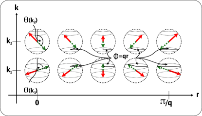
Figure 1: (Color online) The effects of the spin rotation ${\mathcal{U}\!\left(\boldsymbol{r};\boldsymbol{k}\right)}$ on pure spin-up (dashed arrow) or pure spin-down (solid arrow) natural orbitals (plane waves) for two momenta $\boldsymbol{k}_{1/2}$. The angle $\theta_{\boldsymbol{k}}$ specifies the cone on which the spin is rotating. The position on the cone is given by the angle $\phi\!\left(\boldsymbol{r}\right)=\boldsymbol{q}\!\cdot\!\boldsymbol{r}$, which is the same for all natural orbitals.

In previous studies within RMDFT Lathiotakis et al. (2007, 2009) it was assumed that the 1-RDM exhibits the symmetries present in the Hamiltonian, i.e. , the NOs are pure spin-up(down) plane waves, while here we use orbitals of the form of Eq. (14) as NOs for our RDMFT treatment of the UEG. The spin-spiral wave vector $\boldsymbol{q}$ and the angle $\theta_{\boldsymbol{k}}$ will be treated as variational parameters for the NOs. It can easily be verified that the NOs of Eq. (14) form a complete and orthonormal set and that the corresponding electron density ${\rho\equiv 3/\!\left(4\pi r_{s}^{3}\right)}$, given in terms of the Wigner-Seitz radius $r_{s}$, is still spatially constant. The magnetization of the UEG is defined by

$$\boldsymbol{m}\!\left(\boldsymbol{r}\right)\equiv -\frac{1}{2}\sum_{\sigma\sigma^{\prime}}\left\langle\Psi\right|\hat{\psi}^{\dagger}_{\sigma^{\prime}}\!\left(\boldsymbol{r}\right)\boldsymbol{\sigma}_{\sigma\sigma^{\prime}}\hat{\psi}_{\sigma}\!\left(\boldsymbol{r}\right)\left|\Psi\right\rangle$$ (18)

$$= -\begin{pmatrix}\mathcal{R}\gamma_{\uparrow\downarrow}\!\left(\boldsymbol{r};\boldsymbol{r}\right)\\ \mathcal{I}\gamma_{\uparrow\downarrow}\!\left(\boldsymbol{r};\boldsymbol{r}\right)\\ \frac{1}{2}\!\left\{\gamma_{\uparrow\uparrow}\!\left(\boldsymbol{r};\boldsymbol{r}\right)-\gamma_{\downarrow\downarrow}\!\left(\boldsymbol{r};\boldsymbol{r}\right)\right\}\end{pmatrix},$$

and varies in space as

$$\boldsymbol{m}\!\left(\boldsymbol{r}\right)= -\begin{pmatrix}A\cos\!\left(\boldsymbol{q}\!\cdot\!\boldsymbol{r}\right)\\ A\sin\!\left(\boldsymbol{q}\!\cdot\!\boldsymbol{r}\right)\\ B\end{pmatrix},$$ (19a)

$$A\equiv \frac{1}{2}\int\!\!\frac{\mathrm{d}^{3}k}{\!\left(2\pi\right)^{3}}\!\left\{n_{1\boldsymbol{k}}-n_{2\boldsymbol{k}}\right\}\sin\!\left(\theta_{\boldsymbol{k}}\right),$$ (19b)

$$B\equiv \frac{1}{2}\int\!\!\frac{\mathrm{d}^{3}k}{\!\left(2\pi\right)^{3}}\!\left\{n_{1\boldsymbol{k}}-n_{2\boldsymbol{k}}\right\}\cos\!\left(\theta_{\boldsymbol{k}}\right),$$ (19c)

i.e. , the $x$- and $y$-components of the magnetization rotate in space along the direction of $\boldsymbol{q}$ with a periodicity given by the wavelength ${q=\left|\boldsymbol{q}\right|}$. This geometry of the magnetization is usually referred to as SSDW .

III Numerical Implementation

Having chosen a functional and having made an ansatz for the NOs, we minimize the functional for the ground-state energy. The functional depends on $n_{b\boldsymbol{k}}$ , $\theta_{\boldsymbol{k}}$ and the spin-spiral wave vector $\boldsymbol{q}$. The contribution $E_{\mathrm{ion}}$ coming from the uniform positive background charge cancels exactly the classical contribution of the interaction energy, since the density is constant. Accordingly the energy per electron reads

$$e_{\alpha}\!\left[n_{b},\theta\right]\!\left(\boldsymbol{q}\right)=t\!\left[n_{b},\theta\right]\!\left(\boldsymbol{q}\right)-w_{\alpha 1}\!\left[n_{b},\theta\right]-w_{\alpha 2}\!\left[n_{b},\theta\right]\;,$$ (20)

with the kinetic energy per electron

$$t\!\left[n_{b},\theta\right]\!\left(\boldsymbol{q}\right)= \frac{1}{2\rho}\int\!\!\frac{\mathrm{d}^{3}k}{\!\left(2\pi\right)^{3}}\Big{\{}\!\!\left(n_{1\boldsymbol{k}}+n_{2\boldsymbol{k}}\right)k^{2}$$

$$-\boldsymbol{q}\!\cdot\!\boldsymbol{k}\!\left(n_{1\boldsymbol{k}}-n_{2\boldsymbol{k}}\right)\cos\!\left(\theta_{\boldsymbol{k}}\right)\!\Big{\}}+\frac{q^{2}}{8}\;,$$ (21)

the energy contribution from exchange-like terms of orbitals with the same $b$ (intra-band exchange)

$$w_{\alpha 1}\!\left[n_{b},\theta\right]= \frac{1}{2\rho}\iint\!\!\frac{\mathrm{d}^{3}k_{1}\mathrm{d}^{3}k_{2}}{\!\left(2\pi\right)^{6}}\frac{4\pi}{\!\left(\boldsymbol{k}_{1}-\boldsymbol{k}_{2}\right)^{2}}$$

$$\times\!\left\{\!\left(n_{1\boldsymbol{k}_{1}}n_{1\boldsymbol{k}_{2}}\right)^{\alpha}+\!\left(n_{2\boldsymbol{k}_{1}}n_{2\boldsymbol{k}_{2}}\right)^{\alpha}\right\}$$

$$\times\cos^{2}\!\left(\frac{\theta_{\boldsymbol{k}_{1}}-\theta_{\boldsymbol{k}_{2}}}{2}\right)\;,$$ (22)

and the energy contribution from exchange-like terms of orbitals with opposite $b$ (inter-band exchange)

$$w_{\alpha 2}\!\left[n_{b},\theta\right]= \frac{1}{2\rho}\iint\!\!\frac{\mathrm{d}^{3}k_{1}\mathrm{d}^{3}k_{2}}{\!\left(2\pi\right)^{6}}\frac{4\pi}{\!\left(\boldsymbol{k}_{1}-\boldsymbol{k}_{2}\right)^{2}}$$

$$\times\!\left\{\!\left(n_{1\boldsymbol{k}_{1}}n_{2\boldsymbol{k}_{2}}\right)^{\alpha}+\!\left(n_{2\boldsymbol{k}_{1}}n_{1\boldsymbol{k}_{2}}\right)^{\alpha}\right\}$$

$$\times\sin^{2}\!\left(\frac{\theta_{\boldsymbol{k}_{1}}-\theta_{\boldsymbol{k}_{2}}}{2}\right)\;.$$ (23)

We assume that the symmetry is only broken along the direction of $\boldsymbol{q}$ which is chosen to be parallel to the $z$-axis. Accordingly we can use cylindrical coordinates in momentum space, i.e. , ${n_{b\boldsymbol{k}}=n_{bk_{\rho}k_{z}}}$ and ${\theta_{\boldsymbol{k}}=\theta_{k_{\rho}k_{z}}}$. We also use the following additional symmetry assumptions

$$n_{bk_{\rho}-k_{z}}= n_{bk_{\rho}k_{z}}\;\;,\;\;n_{1\boldsymbol{k}}\geq n_{2\boldsymbol{k}},$$ (24a)

$$\theta_{k_{\rho}\pm\left|k_{z}\right|}= \frac{\pi}{2}\!\left\{1\mp a_{k_{\rho}\left|k_{z}\right|}\right\},$$ (24b)

with ${0\leq a_{\boldsymbol{k}}\leq 1}$. In this way we guarantee that the energy gain in the part of the energy which explicitly depends on $\boldsymbol{q}$ is maximized. The $z$-component of the magnetization vanishes under these symmetry assumptions (planar spiral).

The configurations

$$n^{\mathrm{PM}}_{1\boldsymbol{k}}= \Theta\!\left(\left|\boldsymbol{k}-\boldsymbol{e}_{z}k_{f}\right|-k_{f}\right)+\Theta\!\left(\left|\boldsymbol{k}+\boldsymbol{e}_{z}k_{f}\right|-k_{f}\right),$$

$$n^{\mathrm{PM}}_{2\boldsymbol{k}}= 0\;,\;a^{\mathrm{PM}}_{\boldsymbol{k}}=1\;,\;\boldsymbol{q}=2k_{f}\boldsymbol{e}_{z}$$ (25a)

$$\mathrm{and}$$

$$n^{\mathrm{FM}}_{1\boldsymbol{k}}= \Theta\!\left(\left|\boldsymbol{k}-2^{1/3}k_{f}\right|\right),$$

$$n^{\mathrm{FM}}_{2\boldsymbol{k}}= 0\;,\;a^{\mathrm{FM}}_{\boldsymbol{k}}=0\;,\;\boldsymbol{q}=0,$$ (25b)

$$k_{f}\equiv \!\left(\frac{9\pi}{4}\right)^{1/3}\frac{1}{r_{s}},$$

which are compatible with Eq. (24), correspond to the non-magnetic (usually in this context called paramagnetic [PM]) and ferromagnetic (FM) state of the UEG within HF, respectively.

When discretizing the integrals of Eqs. (21)-(23) we assume that the ONs $n_{b\boldsymbol{k}}$ and the angles $a_{\boldsymbol{k}}$ are constant within annular regions in $\boldsymbol{k}$-space

$$\Omega_{i}\equiv\Bigl{\{}\boldsymbol{k}\;\left|\;k^{i-}_{\rho}\leq k_{\rho}\leq k^{i+}_{\rho}\;;\;k^{i-}_{z}\leq k_{z}\leq k^{i+}_{z}\right.\Bigr{\}}.$$ (26)

Then the discretized energy contributions are

$$t\!\left[n_{bi},\theta_{i}\right]\!\left(q\right)= \sum_{bi}n_{bi}\mathrm{DKI}_{i}+\frac{q^{2}}{8}$$

$$-q\sum_{i}\!\left(n_{1i}-n_{2i}\right)\cos\!\left(\theta_{i}\right)\mathrm{DQI}_{i}\;,$$ (27a)

$$w_{\alpha 1}\!\left[n_{bi},\theta_{i}\right]= \frac{1}{2}\sum_{bij}\!\left(n_{bi}n_{bj}\right)^{\alpha}\cos^{2}\!\left(\frac{\theta_{i}-\theta_{j}}{2}\right)\mathrm{DXI}_{ij}\;,\;\;\;\;\;\;\;$$ (27b)

$$w_{\alpha 2}\!\left[n_{bi},\theta_{i}\right]= \sum_{ij}\!\left(n_{1i}n_{2j}\right)^{\alpha}\sin^{2}\!\left(\frac{\theta_{i}-\theta_{j}}{2}\right)\mathrm{DXI}_{ij}\;,\;\;\;$$ (27c)

where the integral weights are given by

$$\mathrm{DKI}_{i}\equiv\frac{1}{8\pi^{2}\rho}\iint_{\Omega_{i}}\!\!\mathrm{d}k_{\rho}\mathrm{d}k_{z}\!\left(k_{\rho}^{3}+k_{\rho}k_{z}^{2}\right)$$ (28a)

$$\mathrm{DQI}_{i}\equiv\frac{1}{8\pi^{2}\rho}\iint_{\Omega_{i}}\!\!\mathrm{d}k_{\rho}\mathrm{d}k_{z}\!\left(k_{\rho}k_{z}\right)$$ (28b)

$$\mathrm{DXI}_{ij}\equiv\frac{1}{2\rho}\iiint_{\Omega_{i}}\!\!\frac{\mathrm{d}k_{\rho 1}\mathrm{d}k_{z1}\mathrm{d}\phi_{1}}{\!\left(2\pi\right)^{3}}\iiint_{\Omega_{j}}\!\!\frac{\mathrm{d}k_{\rho 2}\mathrm{d}k_{z2}\mathrm{d}\phi_{2}}{\!\left(2\pi\right)^{3}}$$

$$\times\frac{4\pi k_{\rho 1}k_{\rho 2}}{k_{\rho 1}^{2}+k_{\rho 2}^{2}+\!\left(k_{z1}-k_{z2}\right)^{2}-2k_{\rho 1}k_{\rho 2}\cos\!\left(\phi_{1}-\phi_{2}\right)}\;.$$ (28c)

The integrals (28a) and (28b) are readily solved and the integrals (28c) can ultimately be reduced to elliptic integrals, which are numerically accessible with high accuracy. Since the momenta are treated as continuous variables we stay in the thermodynamic limit. Thus all energies obtained numerically are variational. The error introduced by the discretization is solely due to the assumption that the ${n_{b\boldsymbol{k}}}$ and ${\theta_{\boldsymbol{k}}}$ are constant within the elementary volume elements ${\Omega_{i}}$ and can systematically be reduced by increasing the number of discretization points.

After having discretized the problem, the minimization of the energy functional of Eq. (20) becomes a high-dimensional optimization problem. We use a steepest descent algorithm for the minimization and ensure that the constraints, Eq. (10), are satisfied during the minimization process. Starting from some initial 1-RDM and some initial discretization in momentum space the energy is minimized for a fixed spin-spiral wave vector $\boldsymbol{q}$. Then the discretization is refined in those regions of momentum space where the $n_{bi}$ and/or the $a_{i}$ show the largest variations. The minimization on the refined momentum space mesh starts from a re-initialized 1-RDM in order to prevent dependencies on the result of the minimization on the coarser grid. Finally we compare the total energies at different $\boldsymbol{q}$ in order to determine the optimal spin-spiral wave vector $\boldsymbol{q}_{opt}$ for various densities.

IV Results

IV.1 Hartree-Fock

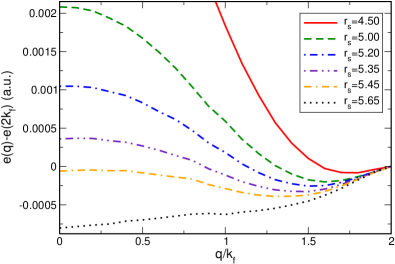
Figure 2: (Color online) Hartree-Fock total energy per electron of the SSDW state as function of the spin-spiral wave vector $q$ at various $r_{s}$. The value $e\!\left(q=2k_{f}\right)$ is subtracted in order to emphasize the behavior of the minimum at different densities. For increasing density (decreasing $r_{s}$) the minimum shifts to higher values of $q_{opt}$ and the energy gained against the paramagnetic state by forming a spin spiral decreases.

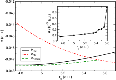
Figure 3: (Color online) Dependence of the energy per electron on $r_{s}$, within the Hartree-Fock approximation, for the paramagnetic, ferromagnetic and SSDW phase in the region of the paramagnetic-ferromagnetic crossover. The inset shows the behavior of the amplitude $A$, defined in Eq. (19b), at the optimal spin-spiral wave vector.

We first use our numerical implementation to investigate Overhauser’s SSDW state in the HF approximation, i.e. , the density-matrix-power functional with ${\alpha=1}$. From the considerations in Eqs. (25) we see that it is sufficient to minimize w.r.t. a 1-RDM whose ONs are only non-zero for orbitals with ${b=1}$ and ${\left|\boldsymbol{q}\right|\in\!\left[0,2k_{f}\right]}$ since both the paramagnetic and the ferromagnetic HF solutions are accessible under these conditions. The minimization at ${q=0}$ and ${q=2k_{f}}$ yields exactly the ONs $n_{bi}$ and angle parameters $a_{i}$ given in Eqs. (25b) and (25a), respectively. Therefore we can read the total energy per particle as function of the spin-spiral wave vector in the following way: $e\!\left(q=0\right)$ is the energy of the ferromagnetic state, $e\!\left(q=2k_{f}\right)$ corresponds to the energy of the paramagnetic state. For intermediate values, $0<q<2k_{f}$, ${e\!\left(q\right)}$ corresponds to a SSDW configuration with ${m_{z}=0}$ (planar spiral). Overhauser’s statement can then be expressed as ${\left.\partial_{q}e\!\left(q\right)\right|_{q=2k_{f}}>0}$, i.e. , the paramagnetic configuration is unstable w.r.t. the formation of a SSDW.

In Fig. 2 we show the dependence of the total energy per particle on the spin-spiral wave vector $\boldsymbol{q}$ for various densities. Consistent with Overhauser’s proof, the derivative of ${e\!\left(q\right)}$ is positive at ${q=2k_{f}}$. It is clear from Fig. 2 that the optimal spin-spiral wave vector moves away from the paramagnetic configuration ${(q=2k_{f})}$ as the density decreases. Furthermore the difference between the total energy at the minimum and the total energy at $q=2k_{f}$ increases with increasing $r_{s}$, i.e. , the instability is more pronounced at lower densities. Below some critical density, however, the ferromagnetic state ($q=0$) becomes the most stable solution. This is not in contradiction with Overhauser’s statement since the spin-spiral state is still lower in energy than the paramagnetic state. A comparison of the energy per electron in the paramagnetic, ferromagnetic and SSDW phase is depicted in Fig. 3. We provide results for the non-collinear magnetic states of the UEG in order to extend the picture given in Ref. Zhang and Ceperley, 2008. It seems that the gain in energy by forming a collinear SDW/CDW state as presented in Ref. Zhang and Ceperley, 2008 is larger compared to the energy gain by forming a SSDW. This is consistent with the qualitative argument already given by Overhauser, that the superposition of a left- and right-rotating SSDW yielding a collinear SDW will increase the gain in energy Overhauser (1962).

To describe the resulting behavior of $q_{opt}\!\left(r_{s}\right)$ we propose a simple, empirical scaling law for the optimal spin-spiral wave vector

$$q_{opt}\!\left(r_{s}\right)=2k_{f}\!\left(1-\!\left(\frac{r_{s}}{r_{0}}\right)^{3}\right)^{\beta},$$ (29)

where ${r_{0}\approx 5.7}$ and ${\beta\approx 0.2}$. The proposed scaling behavior of $q_{opt}$ reproduces the numerical data very accurately as can be seen in Fig. 4. It should be emphasized that we do not find any optimal spin-spiral wave vector ${q_{opt}<k_{f}}$. Note that for densities close to the transition to the ferromagnetic state the optimum wave vector $q_{opt}$ can be quite different from $2k_{f}$ while for higher densities it is very close to this value.

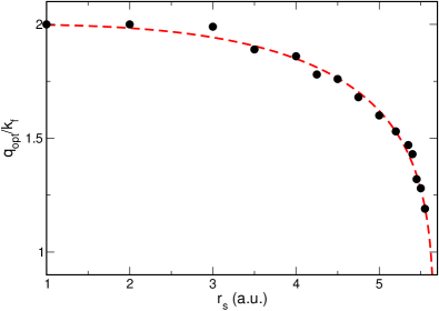
Figure 4: (Color online) Dependence of the Hartree-Fock optimal spin-spiral wave vector $q_{opt}$ on the density, given by $r_{s}$. The proposed approximation by a simple scaling law Eq. (29) is shown as the dashed line.

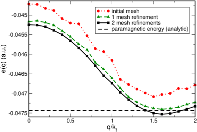
Figure 5: (Color online) Hartree-Fock total energy per electron as function of the spin-spiral wave vector $q$ at the density corresponding to ${r_{s}=5.0}$. The data sets represent results at different discretizations. The dashed horizontal line visualizes the analytic value of the paramagnetic ground state energy. The optimal spin-spiral wave vector is ${q_{opt}\approx 1.6k_{f}}$.

The effect of the refinement of the discretization in momentum space is shown in Fig. 5. By sampling ${n_{bi}}$ and $a_{i}$ more often in regions of higher variations we both lower the energy and reduce the numerical noise in ${e\!\left(q\right)}$. The convergence of the total energy can be inferred from the values ${e\!\left(q=2k_{f}\right)}$ at different discretizations and comparing to the analytic paramagnetic energy. For the case of ${r_{s}=5.0}$ we obtain a spin-spiral energy that is lower than the analytic paramagnetic energy at the optimal value of the spin-spiral wave vector. At higher densities (lower $r_{s}$) the energy gain by forming a SSDW is lower, so we would need a very fine discretization to obtain numerical results lower than the analytic paramagnetic energy. However, considering the numerical value of the paramagnetic energy at the same discretization is sufficient to demonstrate the instability w.r.t. a SSDW formation because the computed energies are variational as discussed in Sec. III. In order to determine the dependence of the optimal spin-spiral wave vector $q_{opt}$ on the density, we therefore refine the momentum space discretization until $q_{opt}$ is converged.

For our numerical results we have verified that the ONs and the angular parameters $a_{i}$ satisfy Overhauser’s self-consistent equations (15) and (16) by iterating them only once. The difference between the angles $a_{i}$ in the occupied regions before and after the iteration is numerically zero for all values of $\boldsymbol{q}$. This means that choosing a spin-spiral wave vector we can always find a solution of the self-consistent equations derived by Overhauser.

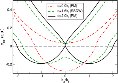
Figure 6: (Color online) Hartree-Fock single-particle dispersion ${(k_{\rho}=0)}$ at ${r_{s}=5.0}$ for the paramagnetic (${q\geq 2k_{f}}$), ferromagnetic (${q=0k_{f}}$) and the SSDW state (${q_{opt}=1.6k_{f}}$). The single-particle energies are shifted such that the dashed horizontal line corresponds to the Fermi energy for all $q$. The difference between the two symmetric minima corresponds to the spin-spiral wave vector $q$. The paramagnetic dispersion may also be viewed as a spin-spiral dispersion with the origin in momentum space shifted by ${\pm q}$ for the different spin channels [cf. Eqs. (25)].

Since the total energy does not depend on the $a_{i}$ in regions where ${n_{bi}=0}$, one self-consistency loop furthermore fixes the angles ${a_{i}}$ in unoccupied regions of $k$-space because they appear only on the left-hand side of Eqs. (16). This is necessary to construct the proper HF dispersions (cf. Fig. 6) also for the unoccupied states. In a complementary work we have investigated the SSDW state using the Optimized-Effective-Potential (OEP) method within the framework of non-collinear Spin-Density-Functional Theory (SDFT)Kurth and Eich (2009). In contrast to our findings within the OEP-DFT framework, i.e. , an effective single-particle theory restricted to local external potentials, here we do not find holes below the Fermi surface (cf. Ref. Kurth and Eich, 2009 for details). This is expected because it was shown in Ref. Bach et al., 1994 that the HF ground state has no holes below the Fermi surface if the interaction is repulsive. Therefore our assumption of occupying only one band is justified.

At the single-particle level we have an intuitive understanding of the instability: as the two distinct spin-up and spin-down regions of the paramagnetic state are squeezed into each other, the orbitals in the overlapping region hybridize. This hybridization then leads to the opening of a direct gap between the HF single-particle dispersions corresponding to ${b=1,2}$ at $k_{z}=0$ as well as to a lowering of both the symmetry and the total energy of the system. The mixing of the spin-up and spin-down orbitals is given by the orbital angles $\theta_{\boldsymbol{k}}$, capable of describing a continuous transition between the paramagnetic and the ferromagnetic state [Eqs. (25a) and (25b) respectively]. The behavior of the orbital angles at the optimal spin-spiral wave vector is shown in Fig. 7.

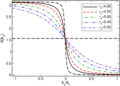
Figure 7: (Color online) Orbital angles ${\theta\!\left(k_{\rho}=0,k_{z}\right)}$ for various densities, specified by $r_{s}$, at the optimal spin-spiral wave vector. The horizontal dashed line corresponds to the orbital angles at ${q=0}$ (ferromagnetic) and the step-like dashed line corresponds to ${q=2k_{f}}$ (paramagnetic). For increasing $r_{s}$ the optimal spin-spiral wave vector becomes smaller, such that the Fermi spheres, separated at ${q=2k_{f}}$, begin to overlap. In order to gain energy the spin-up and spin-down orbitals in the overlapping region hybridize and the orbital angle ${\theta}$ describes the mixing of the spin-up and spin-down states.

IV.2 Correlated Functionals

The density-matrix-power functional reduces to the uncorrelated HF approximation for ${\alpha=1}$ and to the Müller functional for ${\alpha=0.5}$. The latter one is known Lathiotakis et al. (2007) to over-correlate and therefore one expects that decreasing $\alpha$ from ${1\to 0.5}$ increases the amount of correlation in the system. This picture was verified in Ref. Lathiotakis et al., 2009, where an optimal value of ${\alpha\approx 0.6}$ was found in the regions of metallic densities for the paramagnetic UEG. In Fig. 8 the dependence of the total energy per particle at ${r_{s}=5.0}$ is shown for various $\alpha$. It should be noted that the configuration for ${q>2k_{f}}$ cannot be interpreted as the paramagnetic state in the correlated case. This is due to the fact that correlations smear out the sharp step found for the uncorrelated case in the momentum distribution around the Fermi surface (see Ref. Lathiotakis et al., 2007 for details). Therefore at ${q=2k_{f}}$ the (fractionally) occupied regions in momentum space are not necessarily disjoint. Only when the occupied regions separate into two parts the configuration may corresponds to the paramagnetic state. However, the configuration at ${q=0}$ may still be interpreted as the ferromagnetic state.

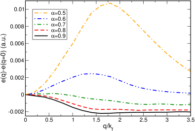
Figure 8: (Color online) Total energies per electron of the SSDW state described with the density-matrix-power functional as a function of the spin-spiral wave vector $q$ for various values of $\alpha$ at ${r_{s}=5.0}$. The total energy per electron at ${q=0}$ is subtracted in order to emphasize the behavior with increasing $q$.

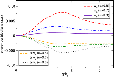
Figure 9: (Color online) Comparison of the correlation energy with the contribution from kinetic plus exchange terms (KEX) for ${\alpha=0.6,0.7,0.8}$ at ${r_{s}=5.0}$. All energy contributions are shifted such that the value at ${q=0}$ is zero. For decreasing $\alpha$ the minimum in the KEX contribution shifts to higher values of $q$. The correlation contribution however damps out this instability for values of $\alpha$ that yield good total energies at metallic densities.

From Fig. 8 it is clear that the instability w.r.t. a SSDW is still present for ${\alpha=0.9}$. For higher values of $\alpha$ the instability disappears and for ${\alpha=0.5,0.6}$ the energy has a maximum in the SSDW region. Thus for values of $\alpha$ which provide good correlation energies for the UEG in the paramagnetic regime there is no SSDW formation. In order to understand the reason for this it is instructive to look at various contributions to the total energy. In Fig. 9 we compare the correlation energy contribution with the contribution coming from the kinetic and exchange terms. The minimum is still present considering only kinetic and exchange contributions, but for decreasing ${\alpha}$ the correlation contribution damps out the instability more and more. One might suspect that at high densities, where exchange dominates correlations, the instability sustains. Our findings in Sec. IV.1 show that in the HF approximation the energy gain decreases when the density increases, which is consistent with an analytic argument Giuliani and Vignale (2008) that at high densities the energy gain by forming a SDW and/or CDW is overcome by correlations. Furthermore our results indicate that correlation effects dominate the SSDW instability also at intermediate densities.

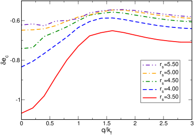
Figure 10: (Color online) Relative correlation energy as a function of the spin-spiral wave vector $q$ for various $r_{s}$ at ${\alpha=0.6}$. Correlations are more important around the ferromagnetic configuration. In the region of the Hartree-Fock SSDW instability correlations have the smallest effect. This indicates why the instability is not sustained when correlations are included at the level of the density-matrix-power functional.

In order to gain some insight into the role of correlations we define the relative correlation energy $\delta e_{c}$ as

$$\delta e^{\alpha}_{c}\equiv\frac{w_{\alpha}-w_{HF}}{\left|e_{\alpha}\right|}\;.$$ (30)

In Fig. 10 we show the dependence of this quantity on the spin-spiral wave vector for the correlation parameter ${\alpha=0.6}$. The absolute value of the relative correlation is smallest in the region of the SSDW instability (${q=k_{f}\to 2k_{f}}$), which explains why the instability is no longer present when correlations are included. Furthermore we can see that the relative correlation is dominant in the region of the ferromagnetic configuration. This can be understood by noticing that the density-matrix-power functional approximates the correlation energy by a prefactor times a Fock integral (most present-day functionals in RDMFT approximate correlations in this wayKollmar (2004); Cioslowski et al. (2003); Cioslowski and Pernal (2005); Csányi and Arias (2000); Csányi et al. (2002); Buijse and Baerends (2002); Gritsenko et al. (2005); Goedecker and Umrigar (1998); Piris (2005); Lathiotakis et al. (2007); Marques and Lathiotakis (2008)). Since Fock integrals imply that equal spins are particularly correlated, one would expect a similar dependence of the relative correlation energy for other RDMFT functionals.

V Summary and Conclusion

We have investigated the instability of the uniform electron gas w.r.t. the formation of a spin-spiral density wave within Reduced-Density-Matrix-Functional Theory, which includes the Hartree-Fock approximation as an important limiting case. To our knowledge this is the first numerical Hartree-Fock study of the spin-spiral state in the electron gas, despite the fact that Overhauser presented his analytical work on the problem more than four decades ago. In Overhauser’s work, the optimal spin-spiral wave vector was not determined. Our study shows that, in contrast to common belief, the optimal spin-spiral wave vector is not always close to ${2k_{f}}$. While at high densities we confirm this value for the optimal wave vector, for lower densities (just before the transition to the ferromagnetic state) the optimal wave vectors even approaches ${k_{f}}$.

Within the framework of Reduced-Density-Matrix-Functional Theory we also studied the effect of correlations on the spin-spiral density wave instability using the recently proposed density-matrix-power functional. Not unexpectedly, we find that the inclusion of correlations suppresses the instability, which is explained by the behavior of the correlation energy in the region of the spin-spiral density wave instability.