The Lorentz force in atmospheres of CP stars: 56 Arietis

Abstract

Context. The presence of electric currents in the atmospheres of magnetic chemically peculiar (mCP) stars could bring important theoretical constrains about the nature and evolution of magnetic field in these stars. The Lorentz force, which results from the interaction between the magnetic field and the induced currents, modifies the atmospheric structure and induces characteristic rotational variability of pressure-sensitive spectroscopic features, that can be analysed using phase-resolved spectroscopic observations.

Aims. In this work we continue the presentation of results of the magnetic pressure studies in mCP stars focusing on the high-resolution spectroscopic observations of Bp star $56$ Ari. We have detected a significant variability of the H$\alpha$, H$\beta$, and H$\gamma$ spectral lines during full rotation cycle of the star. Then these observations are interpreted in the framework of the model atmosphere analysis, which accounts for the Lorentz force effects.

Methods. We used the LLmodels stellar model atmosphere code for the calculation of the magnetic pressure effects in the atmosphere of $56$ Ari  taking into account realistic chemistry of the star and accurate computations of the microscopic plasma properties. The SYNTH3 code was employed to simulate phase-resolved variability of Balmer lines.

Results. We demonstrate that the model with the outward-directed Lorentz force in the dipole$+$quadrupole configuration is likely to reproduce the observed hydrogen lines variation. These results present strong evidences for the presence of non-zero global electric currents in the atmosphere of this early-type magnetic star.

1 Introduction

The atmospheres of magnetic chemically peculiar (mCP) stars display the presence of global magnetic fields ranging in strength from a few hundred G up to several tens of kG (Landstreet, 2001), with the global configurations well represented by dipolar or low-order multipolar components (Bagnulo et al., 2002) and that are likely stable during significant time intervals. The stability of the atmospheres against strong convective motions and the existence of large scale magnetic fields provide a unique conditions for the study of secular evolution of global cosmic magnetic fields and other dynamical processes which may take place in the magnetized plasma. In particular, the slow variation of the field geometry and strength changes the pressure-force balance in the atmosphere via the induced Lorentz force, that makes it possible to detect it observationally and establish a number of important constraints on the plausible scenarios of the magnetic field evolution in early-type stars.

Among the known characteristics of mCP stars, the variability of hydrogen Balmer lines is poorly understood. For some of stars it can be connected with inhomogeneous surface distribution of chemical elements, possible temperature variations and/or stellar rotation (see, for example, discussion in Lehmann et al., 2007). At the same time, some of the magnetic stars demonstrate the characteristic shape of the Balmer line variability that can not be simply described by temperature or abundance effects. For example, Kroll, (1989) showed that at least part of the variability detected in several mCP stars can be attributed to the pressure effects, indicating the presence of a non-zero Lorentz force in their atmospheres.

Different atmosphere models with the Lorenz force were considered by several authors (see review in Valyavin et al., 2004). In this study we follow approaches given by Valyavin et al., (2004) considering the problem in terms of induced atmospheric electric currents interacting with magnetic fields. The authors predicted that the amplitude of the variations in hydrogen Balmer lines seen in real stars can be described if one assumes strong electric currents flowing in upper atmospheric layers of these objects. Later on, Shulyak et al., (2007) (Paper I  hereafter) extended and improved this model to more complicated field geometries and accurate treatment of magnetized plasma properties. Their first direct implementation of new model atmospheres to the analysis of the hydrogen spectra of one of the brightest mCP star $\theta$ Aur showed that their rotational modulation can be induced by the Lorentz force effect, which is not directly connected to the temperature or abundance variation across the stellar surface. The precise analysis of the longitudinal magnetic field variation and subsequent modeling of the magnetic pressure for every observed rotational phase of the star allowed us to constrain the magnitude and the direction of the Lorentz force. In particular, the outward-directed Lorentz force (i.e. directed outside the stellar interior along radius) was found to provide the best fit to observations, in combination with rather strong induced $e.m.f.$ (electro-magnetic force) of about $1\times 10^{-11}$ CGS units which was found to play an important role in the overall hydrostatic structure of the stellar atmosphere.

The knowledge of the direction and the strength of the Lorentz force is important for the understanding of physical mechanisms that are responsible for such strong surface currents and their interaction with global, large-scale magnetic fields (see discussion in Paper I  for more details). Taking this into account and following the pioneering work by Kroll, (1989), we have initiated a new spectroscopic search of hydrogen line variability in a number of magnetic main-sequence stars (Valyavin et al., 2005).

In this paper we present the phase-resolved high-resolution observations of one of the weak-field ($|$$\langle B_{\rm z}\rangle$$|$ $<$ 500 G) mCP star $56$ Ari (HD 19832). We detected significant variation of the Balmer line profiles and interpreted it in terms of the non-force-free magnetic field configuration.

The overview of observations will be presented in the next section. Then, in Sect. 3 we will give a short description of the model used to simulate the effects of the magnetic pressure. Main results will be summarized in Sect. 4 with conclusions and discussion given in Sect. 5 and 6 respectively.

2 Observations

Observations of $56$ Ari were carried out with the BOES echelle spectrograph installed at the $1.8$ m telescope of the Korean Astronomy and Space Science Institute. The spectrograph and observational procedures are described by Kim et al., (2000) and by Kim et al., (2007). The instrument is a moderate-beam, fibre-fed high-resolution spectrometer which incorporates 3 STU Polymicro fibres of $300$, $200$, and $80$ $\mu m$ core diameter (corresponding spectral resolutions are $\lambda/\Delta\lambda=30\,000$, $45\,000$, and $90\,000$ respectively). The medium resolution mode was employed in the present study. Working wavelength range is from $3500$Å  to $10\,000$Å.

Seventeen spectra of the star were recorded in the course of $10$ observing nights from 2004 to 2006. Typical exposure times of a few minutes allowed to achieve $S/N\approx 250$–300. Table 1 gives an overview of our observations. Throughout this study we implement ephemeris derived by Adelman et al., (2001) using linear changing period model:

$$JD=2434322.354+\frac{0.7278883}{1+0.7278883\cdot S\cdot(t-t_{\rm 0})},$$ (1)

where $t_{\rm 0}=2434322.354$ and $S=-1.35\cdot 10^{-9}$.

Details related to spectral data reduction and processing, also study of the spectrograph’s stability are presented in Shulyak et al., (2007), and we don’t describe it here. Accuracy of the continuum normalization around Balmer lines is estimated to be approximately $0.2-0.3$%.

Table 1: Observations of $56$ Ari.

No.	JD	Rotation Phase
1	2453250.2191	0.321
2	2453250.3017	0.435
3	2453251.2284	0.708
4	2453251.3359	0.855
5	2453306.1282	0.128
6	2453306.2942	0.356
7	2453308.0681	0.793
8	2453309.0295	0.114
9	2453309.1620	0.296
10	2453666.0880	0.636
11	2453671.0690	0.478
12	2453671.0860	0.502
13	2453759.0098	0.290
14	2453760.0284	0.689
15	2453760.9714	0.985
16	2453762.0026	0.402
17	2453762.9682	0.728

3 Model

3.1 General equations and approximations

In this section we follow the approach and methods outlined previously in Paper I. However, for the sake of explanation, we find it useful to state here some of the general assumptions used in the modeling procedure:

1. The stellar surface magnetic field is axisymmetric and is dominated by dipolar or dipole+quadrupolar component in all atmospheric layers.

2. The induced $e.m.f.$  has only an azimuthal component, similar to that described by Wrubel, (1952), who considered decay of the global stellar magnetic field. In this case the distribution of the surface electric currents can be expressed by the Legendre polynomials $P^{1}_{n}(\mu)$, where $n=1$ for dipole, $n=2$ for quadrupole, etc., and $\mu=\cos\theta$ is the cosine of the co-latitude angle $\theta$ which is counted in the coordinate system connected to the symmetry axis of the magnetic field.

3. The atmospheric layers are assumed to be in static equilibrium and no horizontal motions are present.

4. Stellar rotation, Hall’s currents, ambipolar diffusion and other dynamical processes are neglected.

Taking these approximations into account and using Maxwell equation for field vectors and Ohm’s law, one can write the hydrostatic equation in the form

$$\frac{\partial P_{\rm total}}{\partial r}=-\rho g\pm\frac{1}{c}\lambda_{\rm\perp}\sum_{n}c_{n}P^{1}_{n}(\mu)\sum_{n}B^{(n)}_{\rm\theta}=-\rho g_{\rm eff}.$$ (2)

Obtaining this equation we used the superposition principle for field vectors and the solution of Maxwell equations for each of the multipolar components following Wrubel, (1952). We also suppose that $\@vec{E}\perp\@vec{B}$. Here $c_{n}$ represents the effective electric field generated by the $n$-th magnetic field component at the stellar magnetic equator and $B_{\rm\theta}$ is the horizontal field component. The signs “+” and “–” refer to the outward- and inward-directed Lorentz forces, respectively.

We note that the values of $c_{n}$ are free parameters to be found by using our model. These values represent the fundamental characteristics that can be used for building self-consistent models of the global stellar magnetic field geometry and its evolution. Thus, an indirect measurement of these parameters via the study of the Lorentz force is of fundamental importance for understanding the stellar magnetism.

Calculation of the electric conductivity $\lambda_{\rm\perp}$ is carried out using the Lorentz collision model where only binary collisions between particles are allowed which is a good approximation for a low density stellar atmosphere plasma. The detailed description and basic relationships of this approach are given in Paper I.

From the Eq. (2) it is seen that, in the presence of electric currents and magnetic field, the rotation of a star can produce phase-dependent Lorentz-force term (due to a variation of $B^{(n)}_{\theta}$ and $\lambda_{\rm\perp}$), which will in turn modify the hydrostatic structure of the atmosphere, manifesting itself as a variation of pressure-sensitive spectral lines.

3.2 Model atmospheres with Lorentz force

Our calculations were carried out with the stellar model atmosphere code LLmodels  developed by Shulyak et al., (2004). At each iteration the code calculates electric conductivity in all atmospheric layers using all available charged and neutral plasma particles. The conductivity is then used to evaluate the magnetic contribution to the magnetic gravity and to execute temperature and mass correction procedure.

The input parameters for the calculation of magnetic pressure are the direction of the Lorentz force (inward- or outward-directed), $e.m.f.$  at the stellar equator, mean surface magnetic field modulus $\langle\@vec{B}\rangle$, and the product of the two sums in Eq. (2) containing contribution from all considered multipolar components for every single rotational phase of the star.

As can be seen from Eq. (2), there is some critical value of $c_{n}$ that may produce unstable solution in the case of the outward-directed Lorentz force. Such models cannot be considered in the hydrostatic equilibrium approximation introduced above and were deemed non-physical in our calculations. Thus, for each set of models, we restricted $c_{n}$ values to ensure static equilibrium.

The atomic line list was extracted from the VALD database (Piskunov et al., 1995; Kupka et al., 1999), including all lines originating from the predicted and observed energy levels. This line list was used as input for the lines opacity calculation in the LLmodels  code.

4 Numerical Results

4.1 Model atmosphere parameters of $56$ Ari

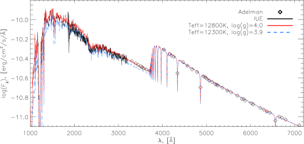
Figure 1: Comparison of the observed and computed spectral energy distributions of $56$ Ari. Theoretical models correspond to $T_{\rm eff}=12\,300$ K, $\log(g)=3.9$ and $T_{\rm eff}=12\,800$ K, $\log(g)=4.0$. The model fluxes have been convolved with an $FWHM$ = 10 Å  Gaussian kernel for a better view.

The model atmosphere parameters, $\log(g)$ and $T_{\rm eff}$, were determined using theoretical fit of the hydrogen Balmer lines and spectral energy distribution. It was constructed by combining the average of the optical spectrophotometric scans obtained by Adelman, (1983) and low dispersion UV spectrograms from the IUE INES database. For modeling the hydrogen H$\beta$ and H$\gamma$ line profiles we used the mean spectrum of $56$ Ari  averaged other all 17 observed rotational phases. The projected rotational velocity $v\sin i$ = 160 km s^-1  was taken from Hatzes, (1993). Ryabchikova, (2003) used the same value in a more recent Doppler imaging study. Individual abundances of several chemical elements, listed in Table 2, were determined as described below (Sect. 4.3).

Table 2: Abundances (in $\log N_{\rm el}/N_{\rm total}$) of $56$ Ari, used for determination of model atmosphere parameters.

	He	Mg	Al	Si	Fe
$56$ Ari	-2.10	-5.51	-6.17	-3.53	-4.09
Sun	-1.10	-4.51	-5.67	-4.53	-4.59

Synthetic Balmer line profiles were calculated using the SYNTH3  program (Kochukhov, 2007), which incorporates recent improvements in the treatment of the hydrogen line opacity (Barklem et al., 2000). The stellar energy distribution and Balmer lines are approximated best with the following parameters: $T_{\rm eff}=12\,800\pm 300$ K, $\log(g)=4.0\pm 0.05$. Note that such high accuracy of the determined parameters is just an internal accuracy obtained from our technique, which we used to fit the data. Real parameters may be slightly different from the obtained ones due to various systematic error sources, but this does not play a significant role in our study.

Comparisons of the observations and model predictions are presented in Figs. 1 and 2. We transformed Adelman’s spectrophotometric observations to the absolute units following Lipski & Stȩpień, (2008). Since the absolute calibration of IUE fluxes around their red end have substantial uncertainties (see Lipski & Stȩpień, 2008), we scaled the IUE fluxes by $\approx$ 10% to match the Adelman’s data in the near-UV region. This correction is comparable to the offset between alternative flux calibrations suggested for the IUE data (García-Gil et al., 2005). Applying the correction ensured that the IUE spectra are smooth continuation of the optical spectrophotometry. Then the theoretical fluxes can be adjusted to fit the combined set of observations. Lipski & Stȩpień, (2008) also noted the discrepancy between observations in visual and UV, but did not do any attempts to correct it. This is why their final effective temperature of $56$ Ari  was found to be $T_{\rm eff}=12\,250$ K resulting from the fact that ignoring the obviously spurious offset between the observed datasets one needs a lower $T_{\rm eff}$ to fit the IUE fluxes simultaneously with Adelman’s fluxes redward of the Balmer jump. As an example we also show in Fig. 1 theoretical flux obtained from the $T_{\rm eff}=12\,300$ K, $\log(g)=3.9$ model which fits reasonably well the hydrogen Balmer lines (see Fig. 2), but fails to reproduce either Adelman’s or IUE data.

Photometric observations in the Strömgren and UBV systems also point to the higher $T_{\rm eff}$ and $\log(g)$ of $56$ Ari. For instance, comparing theoretically computed color-indices with observations of Hauck & Mermilliod, (1998) and Nicolet, (1978) we find that observed photometric parameters ($b-y=-0.052$, $c_{\rm 1}=0.55$, $B-V=-0.12$, $U-B=-0.42$) are best fitted with $T_{\rm eff}=12\,800$ K, $\log(g)=4.0$ model ($b-y=-0.052$, $c_{\rm 1}=0.60$, $B-V=-0.12$, $U-B=-0.43$) rather than more cooler $T_{\rm eff}=12\,300$ K, $\log(g)=3.9$ model ($b-y=-0.048$, $c_{\rm 1}=0.67$, $B-V=-0.12$, $U-B=-0.38$).

Finally, recent studies by Kochukhov et al., (2005) and Khan & Shulyak, (2006) showed that the effects of Zeeman splitting and polarized radiative transfer on the model atmosphere structure and shapes of hydrogen line profiles are less than $0.1$% for magnetic field intensities around $1$ kG, so they can be safely neglected in the present investigation.

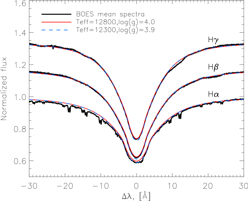
Figure 2: Comparison of the observed and computed H$\alpha$, H$\beta$, and H$\gamma$ line profiles.

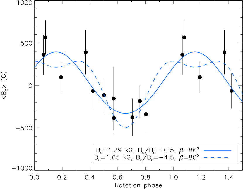
Figure 3: Comparison of the longitudinal field observations of $56$ Ari (symbols) and the model curves for $i=60\degr$ and two extreme values of the $B_{\rm q}/B_{\rm d}$ parameter (lines).

4.2 Magnetic-field geometry

To calculate the Lorentz force effects, it is essential to specify the magnetic-field geometry (see Eq. (2)). For this purpose we made use of the longitudinal magnetic field measurements obtained by Borra & Landstreet, (1980) using H$\beta$ photopolarimetric technique. The authors observed a smooth single-wave $\langle B_{\rm z}\rangle$ variation with rotation phase and concluded that it is probably caused by a dipole inclined to the rotation axis of the star.

Generalizing this work, we have approximated the magnetic-field topology of $56$ Ari by a combination of the dipole and axisymmetric quadrupole magnetic components. We also assumed that the symmetry axes of the dipole and quadrupole magnetic fields are parallel. Thus, the magnetic model parameters include the polar strength of the dipolar component $B_{\rm d}$, relative contribution of the quadrupole field $B_{\rm q}/B_{\rm d}$, magnetic obliquity $\beta$, and inclination angle $i$ of the stellar rotation axis with respect to the line of sight. The last parameter can be estimated from the usual oblique rotator relation connecting stellar radius, rotation period, and $v\sin i$. Employing the recently revised Hipparcos parallax of $56$ Ari, $\pi=6.49\pm 0.76$ mas (van Leeuwen, 2007), $T_{\rm eff}$ = 12800 K and bolometric correction $BC=-0.74$ determined by Lipski & Stȩpień, (2008), we found a stellar radius $R=2.8\pm 0.4$ $R_{\odot}$ and inclination angle $i=57\pm 13\degr$. However, the previous Doppler imaging studies of Hatzes, (1993) and Ryabchikova, (2003) favoured the value of $i=70\degr$. Consequently we decided to explore the model parameters for the entire range of $i=50$–70°.

The remaining free parameters of the magnetic field model were determined with the least-square fit of the observed $\langle B_{\rm z}\rangle$ variation (Borra & Landstreet, 1980). Compared to $\theta$ Aur investigated in Paper I, the longitudinal magnetic field curve of $56$ Ari is poorly defined due to large observational errors and a relatively small number of measurements. In this situation the acceptable solutions for the magnetic field geometry fall in a rather wide range: from $B_{\rm q}/B_{\rm d}=0.5$ to $B_{\rm q}/B_{\rm d}=-5$ for $i=50^{\circ}$, to $B_{\rm q}/B_{\rm d}=-4.5$ for $i=60^{\circ}$, and to $B_{\rm q}/B_{\rm d}=-4$ for $i=70^{\circ}$ (Fig. 3). The corresponding dipolar field strength range is $B_{\rm d}=1.3$–1.8 kG and magnetic obliquity is $\beta=70$–90°. The lowest $\chi^{2}_{\nu}\equiv\chi^{2}/\nu$ was found between $B_{\rm q}/B_{\rm d}=[-1.5,-3]$ with the average value $\chi^{2}_{\nu}\approx 0.66$ while $\chi^{2}_{\nu}\approx 0.71$ for other geometries: with such a small difference we conclude that all the considered magnetic field geometries are equally possible.

4.3 Effects of horizontal abundance distribution

We used spectrum synthesis calculations to access chemical properties of the atmosphere of $56$ Ari. Abundances of He, Al, Mg, Si, and Fe were determined by fitting SYNTH3 spectra to the average observations of the star. Results of this analysis, summarized in Table 2, indicate that He, Al and Mg are deficient in the atmosphere of $56$ Ari with respect to the solar chemical composition. Fe is moderately overabundant while Si is strongly enhanced. Abundance of Cr cannot be determined reliably, but since no prominent Cr ii lines are present in the spectrum of $56$ Ari, we concluded that its overabundance is most likely smaller than that of Fe.

In addition to the mean abundances analysis we interpreted variation of the phase-resolved spectra using the Doppler imaging (DI) technique (Kochukhov et al., 2004). Details of this work will be presented in a separate publication. In the present paper we are only concerned with the possible effect of the horizontal abundance variations on the hydrogen line profiles. Effects of the possible vertical stratitification of chemical elemets are ignored because for the purpose of our study they will not differ much from the effects of horizontal abundance inhomogeneities. By deriving surface-resolved abundances we effectively account for the line opacity variation which would be introduced by chemical stratification.

Among the elements mentioned above only Mg and Si show strong line profile variations. Therefore, we reconstructed abundance maps of Si using the red doublet Si ii 6347, 6371 Å and Mg using the 4481 Å line. The modeling of the latter region also included the He i 4471 Å line, which allowed us to estimate potential influence of the He abundance variation on the model atmosphere structure and hydrogen line profile behaviour.

Analysis of Si, He, and Mg demonstrated that horizontal abundance inhomogeneities give a negligible contribution to the hydrogen line profile variation. We have computed model atmospheres with the surface-averaged abundances for each rotational phase of the star. Figure 4 shows that the resulting standard deviation of the synthetic profiles is minute compared to the variation observed in the line wings of H$\alpha$, H$\beta$, and H$\gamma$.

Much larger abundance gradients of the iron peak elements are required to induce a noticeable modulation of the hydrogen line profiles during rotation cycle. The dashed line in Fig. 4 shows results of the numerical experiment where we have assumed that Fe has the same horizontal distribution as Si but with 10 times higher contrast. This calculation contradicts the actual observations since the Fe lines in $56$ Ari are varying weakly and differently from Si, but it represents a useful illustration of the impact of chemical inhomogeneities. One can see that the metal abundance spots lead to the variation of the depth of hydrogen line cores, while in $56$ Ari we see changes in the line wings. Thus, following Paper I and Kroll, (1989), we are led to conclude that the chemical spots can not contribute to the observed Balmer line wing variations.

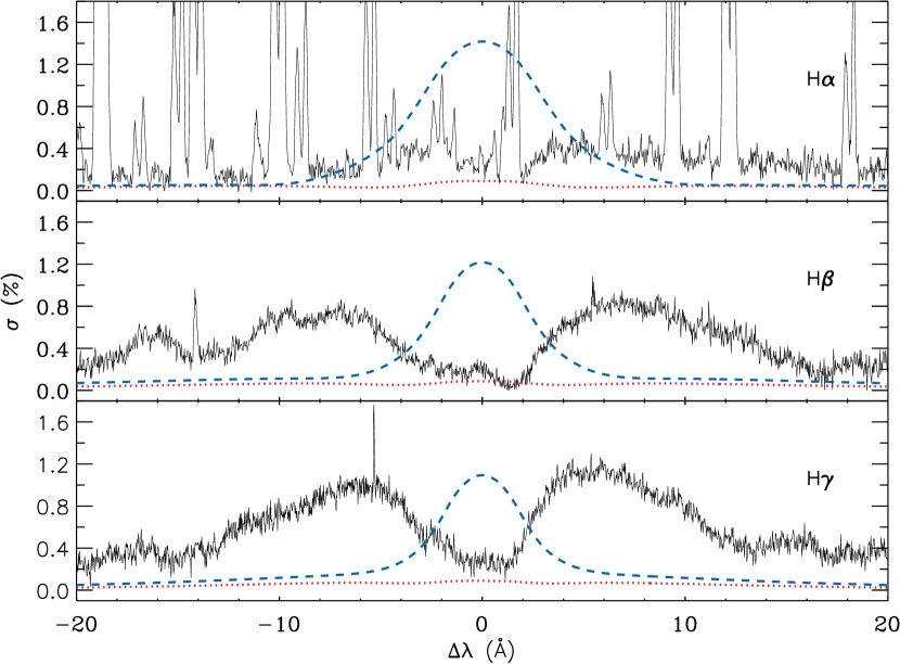
Figure 4: The standard deviation $\sigma$ at the H$\alpha$, H$\beta$, and H$\gamma$ lines. Observations are shown by solid lines. Dotted line – variability due to inhomogeneous element distributions in $56$ Ari. The additional effect of the hypothetical extreme horizontal Fe gradient is shown by the dashed line (see text for explanations).

4.4 The Lorentz force

To predict the phase-resolved variability in hydrogen line profiles both the inward- and outward-directed Lorentz forces are examined through the model atmosphere calculations. The actual magnetic input parameters of computations with the LLmodels  code include the sign of the Lorentz force, magnetic field modulus $B$, and the product of two sums $\sum c_{n}P^{1}_{n}\sum B^{(n)}_{\rm\theta}$ (see Eq. 2). We take the last two parameters to be disk-averaged at the individual rotation phases incorporating them in 1D stellar atmosphere code. The corresponding phase curves of the magnetic parameters relevant for our calculations are illustrated in Fig. 6.

Taking into account the large variety of possible solutions for the surface magnetic field geometry (see Sect. 4.2) we calculated a number of model grids with the outward- and inward-directed Lorentz force and $B_{\rm q}/B_{\rm d}$ ranging from $0.5$ to $-4.5$ with a step of $0.5$.

The calculations showed that, in order to reproduce the amplitudes of the observed standard deviations due to the profile variations, the effective electric field should be in the range $c_{1}=1\times 10^{-10}-5\times 10^{-10}$ CGS in the case of the inward-directed Lorentz force and $c_{1}=1.2\times 10^{-11}-1\times 10^{-10}$ CGS in the case of the outward-directed Lorentz force. Under the assumption of a purely dipolar configuration these values are: $c_{1}=5\times 10^{-10}$ CGS for inward-directed and $c_{1}=7.5\times 10^{-11}$ CGS for outward-directed Lorentz forces.

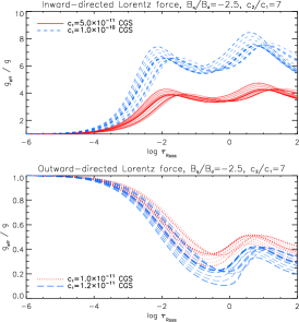
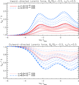
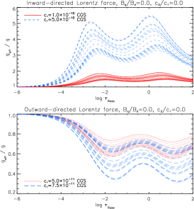
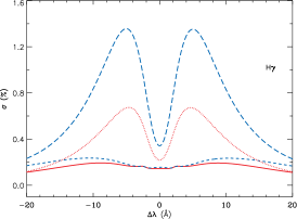
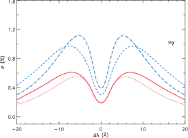
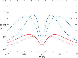
Figure 5: The effective acceleration as a function of the Rosseland optical depth for different rotation phases calculated for several magnetic field configurations and induced $e.m.f.$ The resulting standard deviations around H$\gamma$ line are shown in the bottom panel.

Not for all models considered in our study it was possible to fit the amplitude of the observed standard deviation with the inward-directed Lorentz force. This is true for models with $B_{\rm q}/B_{\rm d}>-1$, where the changes in longitudinal magnetic field and magnetic field modulus result in very narrow phase-resolved variations in magnetic force term. As an example, the left panel of Fig. 5 illustrates the run of the $g_{\rm eff}$ with the Rosseland optical depth in the atmosphere of $56$ Ari ($B_{\rm q}/B_{\rm d}=-2.5$) for inward- and outward directed Lorentz forces computed under different assumptions about induced electric field. An increase of the $e.m.f.$ value by a factor of two considerably changes the amplitude of the effective gravity, but the computed standard deviation does not change much (see lower left panel of Fig. 5). This is why even a large increase of $e.m.f.$ does not reveal itself in a standard deviation plot. Obviously, the situation may change once a more complex geometry of the magnetic field is introduced, however it is connected with the introduction of additional free parameters making the fitting procedure ambiguous. In contrast, the outward-directed magnetic force seems to have a larger impact on the model pressure structure: varying $e.m.f.$ value from $1\times 10^{-11}$ CGS to $1.2\times 10^{-11}$ CGS changes the amplitude of standard deviation by about a factor of two or more.

The amplitude of the standard deviation around hydrogen lines strongly depends on the magnitude of the inward-directed Lorentz force for different magnetic field geometries. For instance, the middle panel of Fig. 5 illustrates standard deviations for the model with $B_{\rm q}/B_{\rm d}=-0.5$: changing induced $e.m.f.$ by a factor of two considerably increases the amplitude of the standard deviation. Similarly, the right panel of Fig. 5 shows the predicted variations for the purely dipolar model.

4.5 Comparison with the observations

In the following we compare the residual theoretical and observed Balmer lines with model predictions based on different assumptions about the magnetic field geometry and the direction of the Lorentz force. The residuals are obtained by subtracting a spectrum at a reference phase ($\phi=0.114$ where the Balmer profiles have the largest widths) from all the other spectra. Figure 7 illustrates residual H$\alpha$, H$\beta$, and H$\gamma$ line profiles for each of the observed rotation phases. The positive sign of the residuals implies that the lines at the current phase are narrower than those obtained at the reference phase. It is seen that the characteristic behaviour of hydrogen lines demonstrates a single wave variation with the most noticeable effect at phases between $\phi=0.402$ and $\phi=0.855$. The effect is also seen in the red wings of lines at $\phi=0.985$, however it is smeared out in the blue wing. We emphasize that this systematic asymmetry, with the blue wing lying below the red one, is observed for all three studied Balmer lines. Inaccuracy of the spectrum processing can be one of the reasons for this effect. However, our data reduction is identical to the analysis of $\theta$ Aur (see Shulyak et al., 2007), which shows no such asymmetry. Thus, we suspect that the asymmetry may also have physical origin due to non-stationary, magnetically-channeled stellar wind from the surface of 56 Ari. Very fast rotation and a relatively high temperature of this star make it plausible that its wind produces the variable, obscured P-Cyg feature distorting blue wings of the Balmer lines. The presence of a weak feature approximately $2.5$Å  blueward the line center seen for all three hydrogen lines could also be an argument for the wind (for H$\gamma$ line the presence of this feature could alternatively be explained by absorption in Ti ii and Fe ii lines, however in case of H$\beta$ there are no spectral lines that could contribute to this feature). Nevetheless, despite these problems introduced by an unknown physical process, the characteristic shape of the Lorentz force induced variability is clearly seen in the hydrogen lines of $56$ Ari, making it possible to perform the analysis in the framework of our modeling approach.

None of the tested theoretical models appeared to fit the observed variability in all phases, but still generally describes the data more or less reasonably well for more than half of them (see, for example, Model 1 or Model 4). Varying the magnetic field geometry and the ratio of induced dipolar and quadrupolar equatorial $e.m.f.$’s ($c_{2}/c_{1}$), we could achieve a good agreement for a certain phase interval only: either it was possible to fit the observations around phase $\phi=0.5$ or for other phases only. As an example, in Fig. 7 we plot some of the theoretical predictions for models that provide a more or less reasonable fit to the observations. In particular, models with the outward-directed Lorentz force are shown for the following configurations:

• $B_{\rm q}/B_{\rm d}=-2.5$, $c_{1}=1.2\times 10^{-11}$ CGS, $c_{2}/c_{1}=7.0$ (Model 1),

• $B_{\rm q}/B_{\rm d}=-4.5$, $c_{1}=1.2\times 10^{-11}$ CGS, $c_{2}/c_{1}=7.0$ (Model 2),

• $B_{\rm q}/B_{\rm d}=+0.5$, $c_{1}=9.0\times 10^{-11}$ CGS, $c_{2}/c_{1}=0.1$ (Model 3).

Also, the model with the inward-directed Lorentz force is presented:

• $B_{\rm q}/B_{\rm d}=-1.0$, $c_{1}=5\times 10^{-10}$ CGS, $c_{2}/c_{1}=2$ (Model 4)

For all plotted models the inclination angle $i=50^{\circ}$ was assumed. Taking $i=70^{\circ}$ does not change much the disc-integrated parameters of the magnetic field and thus leads to essentially the same picture of the hydrogen lines variation (see below).

Models 1 and 2 have the same parameters except the strength of quadrupolar magnetic field component. They produce almost the same fit to the observed variations, and in the same manner are not able to fit phases at $\phi=0.636$ and above (Although Model 2 gives systematically a little bit better fit there). Note that models with $B_{\rm q}/B_{\rm d}<-1.5$ give the same kind of the fit, but we do not plot them here to avoid overcrowding the plot. At the same time, Model 3 seem to be a preferable one for these phases, however it fails to fit observations at phases $\phi=0.435,0.478,0.502$, and gives enormously high effect at phases $\phi=0.321$ and down to zero. This is true also for the Model 4 with inward-directed Lorentz force. This model fits reasonably well such phases as $\phi=0.689,0.708$, but yields the line wings that are generally too wide comparing with observed ones. Thus, of the two possible directions of the Lorentz force in our model we consider an outward-directed Lorentz force as the more reasonable choice to describe observations of $56$ Ari. Due to problems with telluric lines the continuum normalization around H$\alpha$ line is substantially inaccurate comparing to other lines and it is not possible to distinguish between different models there.

Testing models with different magnetic field parameters we tried to find those that predict a single-wave variation of the magnetic force term over the rotation cycle, as indicated by observations. Moreover, its run is likely to have a wide plato around $\phi=0.5$ and drop rapidly close to $\phi=0$ and $\phi=1$ to fit observations (see Fig. 7). By varying the parameters $B_{\rm q}/B_{\rm d}$ and $c_{2}/c_{1}$ (with the fixed $i$ and $\beta$) we succeeded to find sets of parameters that give this kind of plato, but in all cases it appears to be not as wide as it is needed to fit observations in all phases. This is illustrated in Fig. 6 where we plot magnetic parameters used for the Lorentz force calculation in some of the models mentioned above as a function of the rotation phase. The right panel in this figure illustrates predictions for the purely dipolar model. It is also seen that the inclination angle $i$ does not play critical role in the present investigation: models with different $i$ would give the same phase-resolved variation in hydrogen lines and any amplitude difference between them can be adjusted by a proper choice of a $c_{1}$ parameter.

In this investigation we focused analysis on the hydrogen lines. It appears that they are most sensitive to the pressure changes introduced by the Lorentz force. As for metal lines, none of the strong Si ii lines visible in the spectrum of $56$ Ari, $\lambda\leavevmode\nobreak\ 5055.98\leavevmode\nobreak\$Å, $5466.48\leavevmode\nobreak\$Å, $5466.89$ Å, $6347.11$ Å  or $6371.37$ Å, exhibits significant variation due to a non-zero Lorentz force. We have tested this by using the magnetic parameters of Model 1 (which has the largest amplitude of the $g_{\rm eff}$ variation, see Fig. 5) and recomputing spectrum models for every phase with the mean abundances. We find no detectable changes in the line wings and less than $1$% difference in the line cores between models with and without Lorentz force. This difference is likely to be due to the differences in the temperature distribution of these two models. No visible phase-dependent changes can be seen in the spectra corresponding to the models with Lorentz force. These results lead us to the conclusion that, due to their high pressure sensitivity in the predominantly ionized plasma of the atmosphere of such relatively hot star, only the hydrogen lines are useful indicators for the magnetic pressure effects.

Similarly, we find no evidence for the influence of phase-dependent pressure effects on the stellar spectral energy distribution. The maximum difference between models with and without Lorentz force is less than $2$% in Balmer continuum. This corresponds to $\approx$ 0.01 mag difference in $c_{\rm 1}$ color-index and even less for other Strömgren parameters. Thus, variation seen, for example, in the phase-resolved spectrophotometric scans of $56$ Ari published by Adelman, (1983) could not be attributed to the Lorentz force effects but are produced by inhomogeneous abundances and/or other mechanisms.

We note that a strong decrease of $g_{\rm eff}$ evident in Fig. 5 (up to $\approx$ 1 dex around $\log(\tau_{\rm Ross})=0$) compared to the non-magnetic case leads to a relatively small difference in the observed parameters due to a) the fact that this decrease does not affect the entire stellar atmosphere and b) non-local nature of the hydrostatic equation in the presence of depth-dependent $g_{\rm eff}$. The later implies that, for example, one order of magnitude increase of the magnetic gravity results only in three times lower gas pressure for the outward-directed Lorentz force, which is too small to significantly change the opacity coefficient and influence the model structure. The difference between magnetic models for different rotational phases is even smaller since $g_{\rm eff}$ varies maximum by a factor of $\approx$ 2 for Model 1.

Finally, we stress that it is difficult to conclude anything with certainty regarding the preferable model of the magnetic field geometry without additional accurate magnetic observations of the $56$ Ari. Furthermore, other dynamic processes, such as Hall’s currents and particle diffusion, may contribute to the observed variations of hydrogen lines. These processes can not be accounted in our modeling due to their complex nature. Nevertheless, similar to the results of the Paper I, in this study we demonstrate that the observations can be described with a simple geometrical approach under the assumption of strong surface electric currents in the atmosphere of a main-sequence mCP star.

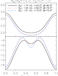
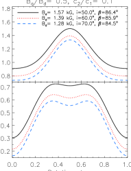
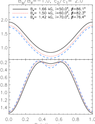
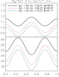
Figure 6: Magnetic field modulus and Lorentz force parameter as a function of rotation phase for several magnetic field models.

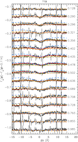
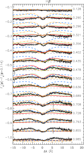
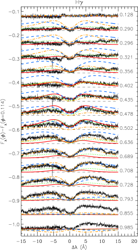
Figure 7: Residual profiles of the H$\alpha$, H$\beta$, and H$\gamma$ lines for each of the observed phase relative to the phase $0.114$. Thin solid line – observations, theoretical profiles are shown for the following models: thick solid line – $B_{\rm q}/B_{\rm d}=-2.5$, $c_{2}/c_{1}=7$ model (outward-directed Lorentz force), dotted line – $B_{\rm q}/B_{\rm d}=-4.5$, $c_{2}/c_{1}=7$ model (outward-directed Lorentz force), dash-dotted line – $B_{\rm q}/B_{\rm d}=0.5$, $c_{2}/c_{1}=0.1$ model (outward-directed Lorentz force), dashed line – $B_{\rm q}/B_{\rm d}=-1.0$, $c_{2}/c_{1}=2$ model (inward-directed Lorentz force). The residual spectra for consecutive phases are shifted in the vertical direction. The thin dashed line gives the zero level for each spectrum.

5 Conclusions

With the use of the high-resolution, phase-resolved observations of a magnetic CP star $56$ Ari and employing modern model atmosphere technique we detected and investigated variations of the Stark-broadened profiles of H$\alpha$, H$\beta$, and H$\gamma$ lines in a framework of a Lorentz force model. Several proofs of the presence of significant magnetic pressure in the atmosphere of $56$ Ari have been found:

• The characteristic shape of the variation during a full rotation cycle of the star corresponds to those described by Kroll, (1989) and other authors as a result of the impact of a substantial Lorentz force (see Paper I and references therein).

• Numerical calculations of the model atmospheres with individual abundances demonstrate that the surface chemical spots cannot produce the observed variability in the hydrogen line profiles of the star.

• Our model shows a reasonable agreement with the observations if the outward-directed magnetic force is applied assuming the dipole+quadrupole magnetic field configuration. Unfortunately, due to large uncertainties in the available observations of the longitudinal magnetic field it was not possible to conclude confidently about the strengths of the quadrupolar component.

• Taking into account a variety of possible solutions, we find that, to fit the amplitude of a phase-resolved variation in H$\alpha$, H$\beta$, and H$\gamma$ lines, the magnitude of an induced equatorial $e.m.f.$ must be in the range $10^{-11}-10^{-10}$ CGS in case of outward-directed Lorentz force and $\sim 5\times 10^{-10}$ in case of inward-directed one.

6 Discussion

$56$ Ari is the second magnetic CP star for which we detected the characteristic variation of the hydrogen Balmer line profiles and performed detailed modeling of the Lorentz force effect. Our previous target, A0p star $\theta$ Aur, also demonstrated significant variability in the hydrogen Balmer lines (see Paper I). However, in the case of $\theta$ Aur, Borra & Landstreet, (1980) provided a much more accurate measurements of the longitudinal magnetic field variations, which allowed us to determine more precisely geometry of its surface magnetic field. Nevertheless, for both stars we find that the outward-directed Lorentz force is needed to explain observations. However the induced $e.m.f.$ for $56$ Ari may differ by an order of magnitude, but this remains uncertain due to poorly known magnetic field geometry.

A single-wave variation of the residual spectra is a characteristic signature for both $\theta$ Aur and $56$ Ari. Since both stars have high inclination angles and magnetic obliquities, in the framework of our Lorentz force model this variation indicates the presence of a more complex magnetic field geometry than a simple dipole. Such a variation can be obtained in the non-dipolar theoretical models by a proper choice of induced $e.m.f.$ for each of the multipolar components (e.g. the $c_{2}/c_{1}$ ratio in the case of dipole$+$quadrupole combination). Furthermore, for both stars the amplitude of the longitudinal magnetic field variation is about $\approx 500$ G, which can be the reason for similar amplitude of the detected Balmer lines variation ($\approx 1$%) since the effective temperatures of stars are different ($T_{\rm eff}$($\theta$ Aur)$=10\,400$ K, $T_{\rm eff}$($56$ Ari)$=12\,800$ K).

Similar to the Paper I, we do not consider here any details about the physical mechanisms that could be responsible for the observed Lorentz force. The final conclusion about the nature of the significant magnetic pressure can only be obtained when more sophisticated models of the magnetic field evolution and its interaction with highly magnetized atmospheric structure will become available and/or alternative models will be tested (however, for some of the estimates see discussion in Shulyak et al., 2007).

In the present work we made use of a simple geometrical 1D model of Lorentz force: the surface averaged values of the transverse magnetic field and the magnetic field modulus are introduced in the hydrostatic equation of the stellar matter. Future investigations can benefit from taking into account 2D effects with direct surface integration of the hydrogen line profiles computed with individual models. This could probably also open a possibility to account for the Hall’s currents. Unfortunately, as it was mentioned above, this is difficult to do at present, but of no way impossible once more computational resources become available.

The dependence of the observed variability in hydrogen lines upon the magnetic field geometry and strength is one of the key element in our investigation. If such a dependence exists, it could bring a number of theoretical constrains about the interaction of the magnetic field with stellar plasma. So far, we have analyzed only two stars with occasionally similar longitudinal magnetic field intensity. Note that we are limited to stars for which the configuration of a magnetic field can be extracted from the literature and which can be observed with highly stable spectrometers like BOES in order to reduce possible errors in spectra processing. Thus, observations of other mCP stars are needed to conclude about the connection between magnetic field and variability seen in Balmer lines.