$n\bar{n}$ transitions in medium

Abstract

The models of $n\bar{n}$ transitions in the medium based on unitary $S$-matrix are considered. The time-dependence and corrections to the models are studied. The lower limits on the free-space $n\bar{n}$ oscillation time are obtained as well.

PACS: 11.30.Fs; 13.75.Cs

Keywords: diagram technique, infrared divergence, time-dependence

*E-mail: nazaruk@inr.ru

1 Introduction

In the standard calculations of $ab$ oscillations in the medium [1-3] the interaction of particles $a$ and $b$ with the matter is described by the potentials $U_{a,b}$ (potential model). ${\rm Im}U_{b}$ is responsible for loss of $b$-particle intensity. In particular, this model is used for the $n\bar{n}$ transitions in a medium [4-10] followed by annihilation:

$$n\rightarrow\bar{n}\rightarrow M,$$ (1)

here $M$ are the annihilation mesons.

In [9] it was shown that one-particle model mentioned above does not describe the total $ab$ (neutron-antineutron) transition probability as well as the channel corresponding to absorption of the $b$-particle (antineutron). The effect of final state absorption (annihilation) acts in the opposite (wrong) direction, which tends to the additional suppression of the $n\bar{n}$ transition. The $S$-matrix should be unitary.

In [11] we have proposed the model based on the diagram technique which does not contain the non-hermitian operators. Subsequently, this calculation was repeated in [12]. However, in [13] it was shown that this model is unsuitable: the neutron line entering into the $n\bar{n}$ transition vertex should be the wave function, but not the propagator, as in the model based on the diagram technique. For the problem under study this fact is crucial. It leads to the cardinal error for the process in nuclei. The $n\bar{n}$ transitions in the medium and vacuum are not reproduced at all. If the neutron binding energy goes to zero, the result diverges (see Eqs. (18) and (19) of Ref. [11] or Eqs. (15) and (17) of Ref. [12]). So we abandoned this model [13]. (In the recent manuscript [14] the previous calculations [11,12] have been repeated. The model and calculation are the same as in [11,12]. Unfortunately, several statements are erroneous [15], in particular, the conclusion based on an analogy with the nucleus form-factor at zero momentum transfer (for more details, see [15]).)

In [16] the model which is free of drawbacks given above has been proposed (model b in the notations of present paper). However, the consideration was schematic since our concern was only with the role of the final state absorption in principle. In Sect. 2 this model as well as the model with bare propagator are studied in detail. The corrections to the models (Sect. 3) and time-dependence (Sect. 4) are considered as well. In addition, we sum up the present state of the investigations of this problem (Sect. 5).

The basic material is given in Sects. 2 and 5.

2 Models

First of all we consider the antineutron annihilation in the medium. The annihilation amplitude $M_{a}$ is defined as

$$<\!f0\!\mid T\exp(-i\int dx{\cal H}(x))-1\mid\!0\bar{n}_{p}\!>=N(2\pi)^{4}\delta^{4}(p_{f}-p_{i})M_{a}.$$ (2)

Here ${\cal H}$ is the Hamiltonian of the $\bar{n}$-medium interaction, $\mid\!0\bar{n}_{p}\!>$ is the state of the medium containing the $\bar{n}$ with the 4-momentum $p=(\epsilon,{\bf p})$; $<\!f\!\mid$ denotes the annihilation products, $N$ includes the normalization factors of the wave functions. The antineutron annihilation width $\Gamma$ is expressed through $M_{a}$:

$$\Gamma\sim\int d\Phi\mid\!M_{a}\!\mid^{2}.$$ (3)

For the Hamiltonian ${\cal H}$ we consider the model

$${\cal H}={\cal H}_{a}+V\bar{\Psi}_{\bar{n}}\Psi_{\bar{n}},$$

$$H(t)=\int d^{3}x{\cal H}(x)=H_{a}(t)+V,$$ (4)

where ${\cal H}_{a}$ is the effective annihilation Hamiltonian in the second quantization representation, $V$ is the residual scalar field. The diagrams for the model (4) are shown in Fig. 1. The first diagram corresponds to the first order in ${\cal H}_{a}$ and so on.

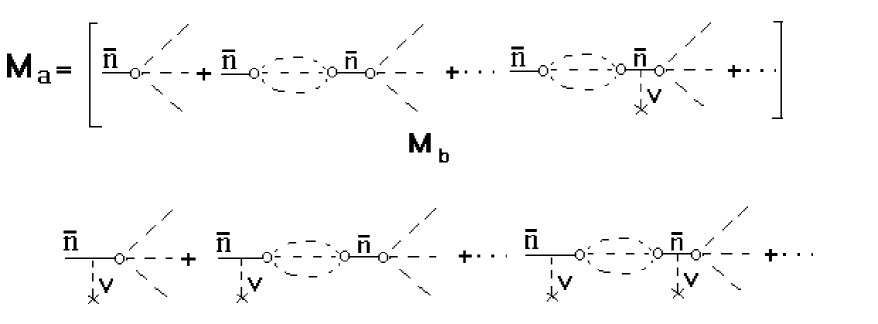
Figure 1: Antineutron annihilation in the medium. The annihilation is shown by a circle

Consider now the process (1). The neutron wave function is

$$n(x)=\Omega^{-1/2}\exp(-ipx).$$ (5)

Here $p=(\epsilon,{\bf p})$ is the neutron 4-momentum; $\epsilon={\bf p}^{2}/2m+U_{n}$, where $U_{n}$ is the neutron potential. The interaction Hamiltonian has the form

$$H_{I}=H_{n\bar{n}}+H,$$ (6)

$$H_{n\bar{n}}(t)=\int d^{3}x(\epsilon_{n\bar{n}}\bar{\Psi}_{\bar{n}}(x)\Psi_{n}(x)+H.c.)$$ (7)

Here $H_{n\bar{n}}$ is the Hamiltonian of $n\bar{n}$ conversion [6], $\epsilon_{n\bar{n}}$ is a small parameter with $\epsilon_{n\bar{n}}=1/\tau$, where $\tau$ is the free-space $n\bar{n}$ oscillation time; $m_{n}=m_{\bar{n}}=m$. In the lowest order in $H_{n\bar{n}}$ the amplitude of process (1) is uniquely determined by the Hamiltonian (6):

$$M=\epsilon_{n\bar{n}}G_{0}M_{a},$$ (8)

$$G_{0}=\frac{1}{\epsilon-{\bf p}^{2}/2m-U_{n}+i0},$$ (9)

${\bf p}_{\bar{n}}={\bf p}$, $\epsilon_{\bar{n}}=\epsilon$. Here $G_{0}$ is the antineutron propagator. The corresponding diagram is shown in Fig. 2a. The annihilation amplitude $M_{a}$ is given by (2), where ${\cal H}={\cal H}_{a}+V\bar{\Psi}_{\bar{n}}\Psi_{\bar{n}}$. Since $M_{a}$ contains all the $\bar{n}$-medium interactions followed by annihilation including antineutron rescattering in the initial state, the antineutron propagator $G_{0}$ is bare. Once the antineutron annihilation amplitude is defined by (2), the expression for the process amplitude (8) rigorously follows from (6). For the time being we do not go into the singularity $G_{0}\sim 1/0$.

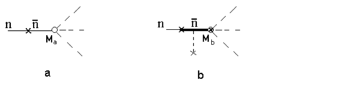
Figure 2: a $n\bar{n}$ transition in the medium followed by annihilation. The antineutron annihilation is shown by a circle. b Same as a but the antineutron propagator is dressed (see text)

One can construct the model with the dressed propagator. We include the scalar field $V$ in the antineutron Green function

$$G_{d}=G_{0}+G_{0}VG_{0}+...=\frac{1}{(1/G_{0})-V}=-\frac{1}{V}=-\frac{1}{\Sigma},$$ (10)

$\Sigma=V$, where $\Sigma$ is the antineutron self-energy. The process amplitude is

$$M=\epsilon_{n\bar{n}}G_{d}M_{b},$$ (11)

$G_{d}M_{b}=G_{0}M_{a}$ (see Fig. 2b). The block in the square braces shown in Fig.1 corresponds to the vertex function $M_{b}$. The models shown in Figs. 2a and 2b we denote as the models a and b, respectively.

In both models the interaction Hamiltonians $H_{I}$ and unperturbed Hamiltonians are the same. If $\Sigma\rightarrow 0$, the model b goes into model a. In this sense the model a is the limiting case of the model b.

We consider the model b. For the process width $\Gamma_{b}$ one obtains

$$\Gamma_{b}=N_{1}\int d\Phi\mid\!M\!\mid^{2}=\frac{\epsilon_{n\bar{n}}^{2}}{\Sigma^{2}}N_{1}\int d\Phi\mid\!M_{b}\!\mid^{2}=\frac{\epsilon_{n\bar{n}}^{2}}{\Sigma^{2}}\Gamma^{\prime},$$ (12)

$$\Gamma^{\prime}=N_{1}\int d\Phi\mid\!M_{b}\!\mid^{2},$$ (13)

where $\Gamma^{\prime}$ is the annihilation width of $\bar{n}$ calculated through the $M_{b}$ (and not $M_{a}$). The normalization multiplier $N_{1}$ is the same for $\Gamma_{b}$ and $\Gamma^{\prime}$. The vertex function $M_{b}$ is unknown. (We recall the antineutron annihilation width $\Gamma$ is expressed through the amplitude $M_{a}$.) For the estimation we put

$$M_{b}=M_{a},\quad\Gamma^{\prime}=\Gamma.$$ (14)

This is an uncontrollable approximation.

The time-dependence is determined by the exponential decay law:

$$W_{b}(t)=1-e^{-\Gamma_{b}t}\approx\Gamma_{b}t=\frac{\epsilon_{n\bar{n}}^{2}}{\Sigma^{2}}\Gamma t.$$ (15)

Equation (15) illustrates the result sensitivity to the value of parameter $\Sigma$.

On the other hand, for $n\bar{n}$ transitions in nuclear matter the standard calculation gives the inverse $\Gamma$-dependence [6-9]

$$W_{{\rm stan}}(t)=2\epsilon_{n\bar{n}}^{2}t\frac{\Gamma/2}{({\rm Re}U_{\bar{n}}-U_{n})^{2}+(\Gamma/2)^{2}}\approx\frac{4\epsilon_{n\bar{n}}^{2}t}{\Gamma},$$ (16)

where $U_{\bar{n}}$ is the antineutron optical potential. The wrong $\Gamma$-dependence is a direct consequence of the inapplicability of the model based on optical potential for the calculation of the total process probability [9]. (The above-mentioned model describes the probability of finding an antineutron only.)

Comparing with (15), one obtains

$$r=\frac{W_{b}}{W_{{\rm stan}}}=\frac{\Gamma^{2}}{4\Sigma^{2}}=25,$$ (17)

where the values $\Gamma=100$ MeV and $\Sigma={\rm Re}U_{\bar{n}}-U_{n}=10$ MeV have been used. Strictly speaking, the parameter $\Sigma$ is uncertain. We have put $\Sigma={\rm Re}U_{\bar{n}}-U_{n}=10$ MeV only for estimation.

The model b leads to an increase of the $n\bar{n}$ transition probability. The lower limit on the free-space $n\bar{n}$ oscillation time $\tau^{b}_{{\rm min}}$ increases as well:

$$\tau^{b}_{{\rm min}}=(3.5-7.5)\cdot 10^{8}\;{\rm s}.$$ (18)

This limit exceeds the previous one (see, for example, Refs. [5-8]) by a factor of five. If $\Sigma\rightarrow 0$, $W_{b}$ rises quadratically. So Eq. (18) can be considered as the estimation from below.

We return to the model shown in Fig. 2a. We use the basis $(n,\bar{n})$. The results do not depend on the basis. A main part of existing calculations have been done in $n-\bar{n}$ representation. The physics of the problem is in the Hamiltonian. The transition to the basis of stationary states is a formal step. It has a sense only in the case of the potential model $H=H_{{\rm pot}}={\rm Re}U_{\bar{n}}-U_{n}-i\Gamma/2=$const., when the Hamiltonian of $\bar{n}$-medium interaction is replaced by the effective mass $H\rightarrow H_{{\rm pot}}=m_{{\rm eff}}$ because the Hermitian Hamiltonian of interaction of the stationary states with the medium is unknown. Since we work beyond the potential model, the procedure of diagonalization of mass matrix is unrelated to our problem.

The amplitude (8) diverges

$$M=\epsilon_{n\bar{n}}G_{0}M_{a}\sim\frac{1}{0}.$$ (19)

(See also Eq. (21) of Ref. [13].) These are infrared singularities conditioned by zero momentum transfer in the $n\bar{n}$ transition vertex. (In the model b the effective momentum transfer $q_{0}=V=\Sigma$ takes place.)

For solving the problem the field-theoretical approach with finite time interval [17] is used. It is infrared free. If $H=H_{{\rm pot}}$, the approach with finite time interval reproduces all the results on the particle oscillations, in particular, the $n\bar{n}$ transition with $\bar{n}$ in the final state. (Recall that our purpose is to describe the process (1) by means of Hermitian Hamiltonian.)

For the model a the process (1) probability was found to be [10,13]

$$W_{a}(t)\approx W_{f}(t)=\epsilon_{n\bar{n}}^{2}t^{2},\quad\Gamma t\gg 1,$$ (20)

where $W_{f}$ is the free-space $n\bar{n}$ transition probability. Owing to annihilation channel, $W_{a}$ is practically equal to the free-space $n\bar{n}$ transition probability. If $t\rightarrow\infty$, Eq. (20) diverges just as the modulus (19) squared does. If $\Sigma\rightarrow 0$, Eq. (15) diverges quadratically as well.

The explanation of the $t^{2}$-dependence is simple. The process shown in Fig. 2a represents two consecutive subprocesses. The speed and probability of the whole process are defined by those of the slower subprocess. If $1/\Gamma\ll t$, the annihilation can be considered instantaneous. So, the probability of process (1) is defined by the speed of the $n\bar{n}$ transition: $W_{a}\approx W_{f}\sim t^{2}$.

Distribution (20) leads to very strong restriction on the free-space $n\bar{n}$ oscillation time [10,13]:

$$\tau^{a}_{{\rm min}}=10^{16}\;{\rm yr}.$$ (21)

3 Corrections

We show that for the $n\bar{n}$ transition in medium the corrections to the models and additional baryon-number-violating processes (see Fig. 3) cannot essentially change the results. First of all we consider the incoherent contribution of the diagrams 3. In Fig. 3a a meson is radiated before the $n\bar{n}$ transition. The interaction Hamiltonian has the form

$$H_{I}=\int d^{3}xg\Psi^{+}_{n}\Phi\Psi_{n}+H_{n\bar{n}}+H.$$ (22)

In the following the background neutron potential is omitted. The neutron wave function is given by (5), were $p=(p_{0},{\bf p})$ and $p_{0}=m+{\bf p}^{2}/2m$.

For the process amplitude $M_{3a}$ one obtains

$$M_{3a}=gG\epsilon_{n\bar{n}}GM^{(n-1)},$$ (23)

$$G=\frac{1}{p_{0}-q_{0}-m-({\bf p}-{\bf q})^{2}/2m+i0},$$ (24)

where $q$ is the 4-momentum of meson radiated, $M^{(n-1)}$ is the amplitude of antineutron annihilation in the medium in the $(n-1)$ mesons. As with model a, the antineutron propagator $G$ is bare; the $\bar{n}$ self-energy $\Sigma=0$. (The same is true for Figs. 3b-3d.)

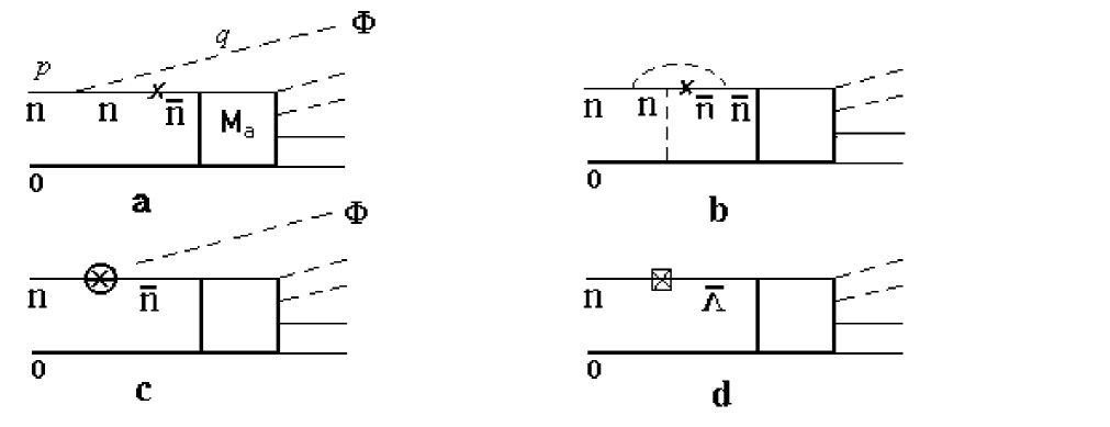
Figure 3: Corrections to the models (a and b) and additional baryon-number-violating processes (c and d)

If $q\rightarrow 0$, the amplitude $M_{3a}$ increases since $G\rightarrow G_{s}$,

$$G_{s}=\frac{1}{p_{0}-m-{\bf p}^{2}/2m}\sim\frac{1}{0}.$$ (25)

(The limiting transition $q\rightarrow 0$ for the diagram 3a is an imaginary procedure because in the vertex $n\rightarrow n\Phi$ the real meson is escaped and so $q_{0}\geq m_{\Phi}$.) The fact that the amplitude increases is essential for us because for Fig. 2a $q=0$. Due to this $G_{0}\sim 1/0$ and $W_{a}\gg W_{b}$.

Let $\Gamma_{3a}$ and $\Gamma^{(n)}$ be the widths corresponding to the Fig. 3a and annihilation width of $\bar{n}$ in the $(n)$ mesons, respectively; $\Gamma=\sum_{(n)}\Gamma^{(n)}$. Taking into account that $\Gamma^{(n)}$ is a smooth function of $\sqrt{s}$ and summing over $(n)$, it is easy to get the estimation:

$$\Gamma_{3a}\approx 5\cdot 10^{-3}g^{2}\frac{\epsilon_{n\bar{n}}^{2}}{m^{2}_{\Phi}}\Gamma\approx\frac{\epsilon_{n\bar{n}}^{2}}{m^{2}_{\Phi}}\Gamma.$$ (26)

The time-dependence is determined by the exponential decay law:

$$W_{3a}(t)\approx\Gamma_{3a}t=\frac{\epsilon_{n\bar{n}}^{2}}{m^{2}_{\Phi}}\Gamma t.$$ (27)

Comparing with (15) we have: $W_{3a}/W_{b}=V^{2}/m^{2}_{\Phi}\ll 1$. So for the model b the contribution of diagram 3a is negligible.

For the model a the contribution of diagram 3a is inessential as well. Indeed, using Eqs. (27) and (20) we get

$$\frac{W_{3a}(t)}{W_{a}(t)}=\frac{\Gamma}{m^{2}_{\pi}t},$$ (28)

where we have put $m_{\Phi}=m_{\pi}$. Consequently, if

$$m^{2}_{\pi}t/\Gamma\gg 1,$$ (29)

and

$$\Gamma t\gg 1$$ (30)

(see (20)) then the contribution of diagram 3a is negligible. For the $n\bar{n}$ transition in nuclei these conditions are fulfilled since in this case $\Gamma\sim 100$ MeV and $t=T_{0}=1.3$ yr, where $T_{0}$ is the observation time in proton-decay type experiment [18].) In fact, it is suffice to hold condition (30) only because it is more strong.

In the calculations made above the free-space $n\bar{n}$ transition operator has been used. This is impulse approximation which is employed for nuclear $\beta$ decay, for instance. The simplest medium correction to the vertex (or off-diagonal mass, or transition mass) is shown in Fig. 3b. In this event the replacement should be made:

$$\epsilon_{n\bar{n}}\rightarrow\epsilon_{m}=\epsilon_{n\bar{n}}(1+\Delta\epsilon),$$ (31)

$\Delta\epsilon=\epsilon_{3b}/\epsilon_{n\bar{n}}$, where $\epsilon_{3b}$ is the correction to $\epsilon_{n\bar{n}}$ produced by the diagram 3b. For the model a the limit becomes

$$\tau^{a}_{{\rm min}}=(1+\Delta\epsilon)10^{16}\;{\rm yr}.$$ (32)

Obviously, the $\Delta\epsilon$ cannot change the order of magnitude of $\tau_{{\rm min}}$ since the $n\rightarrow\bar{n}$ operator is essentially zero-range one. The free-space $n\bar{n}$ transition comes from the exchange of Higgs bosons with the mass $m_{H}>10^{5}$ GeV [5]. Since $m_{H}\gg m_{W}$ ($m_{W}$ is the mass of $W$-boson), the renormalization effects should not exceed those characteristic of nuclear $\beta$ decay which is less than 0.25 [19]. So the medium corrections to the vertex are inessential for us. The same is true for the model b.

Consider now the baryon-number-violating decay $n\rightarrow\bar{n}\Phi$ [20] shown in Fig. 3c. It leads to the same final state, as the processes depicted in Figs. 2, 3a and 3b. Denoting $\mid{\bf q}\mid=q$, for the decay width $\Gamma_{3c}$ one obtains

$$\Gamma_{3c}=\frac{\epsilon_{\Phi}^{2}}{(2\pi)^{2}}\int dq\frac{q^{2}}{q_{0}}G^{2}\Gamma(q),$$ (33)

$q_{0}^{2}=q^{2}+m_{\Phi}^{2}$. The parameter $\epsilon_{\Phi}$ corresponding to the vertex $n\rightarrow\bar{n}\Phi$ is unknown and so no detailed calculation is possible.

The baryon-number-violating conversion $n\rightarrow\bar{\Lambda}$ in the medium [20] shown in Fig. 3d cannot produce interference, since it contains $K$-meson in the final state. For the rest of the diagrams the significant interferences are unlikely because the final states in $\bar{n}N$ annihilation are very complicated configurations and persistent phase relations between different amplitudes cannot be expected. This qualitative picture is confirmed by our calculations [21] for $\bar{p}$-nuclear annihilation. It is easy to verify the following statement: if the incoherent contribution of the diagrams 3a-3c to the total nuclear annihilation width is taken into account, the lower limit on the free-space $n\bar{n}$ oscillation time $\tau_{{\rm min}}$ becomes even better.

To summarise, the contribution of diagrams 3 is inessential for us.

4 Time-dependence

The non-trivial circumstance is the quadratic time-dependence in the model a: $W_{a}\sim t^{2}$. The heart of the problem is as follows. The processes depicted by the diagrams 2b and 3 are described by the exponential decay law. In the first vertex of these diagrams the momentum transfer (Figs. 3a-3c), or effective momentum transfer (Figs. 2b, 3d) takes place. The diagram 2a contains the infrared divergence conditioned by zero momentum transfer in the $n\bar{n}$ transition vertex. This is unremovable perculiarity. This means that the standard $S$-matrix approach is inapplicable [10,13,17]. In such an event, the other surprises can be expected as well. From this standpoint a non-exponential behaviour comes as no surprise to us. It seems natural that for non-singular and singular diagrams the functional structure of the results is different, including the time-dependence. The opposite situation would be strange.

The fact that for the processes with $q=0$ the $S$-matrix problem formulation $(\infty,-\infty)$ is physically incorrect can be seen even from the limiting case $H=0$: if $H_{I}=H_{n\bar{n}}$ (see (6)), the solution is periodic. It is obtained by means of non-stationary equations of motion and not $S$-matrix theory. To reproduce the limiting case $H\rightarrow 0$, i.e. the periodic solution, we have to use the approach with finite time interval.

If the problem is formulated on the interval $(t,0)$, the decay width $\Gamma$ cannot be introduced since $\Gamma=\sum_{f\neq i}\mid S_{fi}(\infty,-\infty)\mid^{2}/T_{0}$, $T_{0}\rightarrow\infty$. This means that the standard calculation scheme should be completely revised. (We would like to emphasise this fact.) The direct calculation by means of evolution operator gives the distribution (20).

Formally, the different time-dependence is due to $q$-dependence of amplitudes. We consider Eq. (23), for instance. If $q$ decreases, the amplitude $M_{3a}$ increase; in the limit $q\rightarrow 0$ it is singular (see (25)). The point $q=0$ corresponds to realistic process shown in Fig. 2a. The $t^{2}$-dependence of this process is the consequence of the zero momentum transfer.

The more physical explanation of the $t^{2}$-dependence is as follows. In the Hamiltonian (22) corresponding to Fig. 3a we put $H=H_{n\bar{n}}=0$. Then the virtual decay $n\rightarrow n\Phi$ takes place. The first vertex of the diagram 3a dictates the exponential decay law of the overall process shown in Fig. 3a. Similarly, in the Hamiltonian (6) corresponding to Fig. 2a, we put $H=0$. Then the free-space $n\bar{n}$ transition takes place which is quadratic in time: $W_{f}(t)=\epsilon_{n\bar{n}}^{2}t^{2}$. The first vertex determines the time-dependence of the whole process at least for small $\Gamma$. We also recall that even for proton decay the possibility of non-exponential behaviour is realistic [22-24].

5 Discussian and summary

The sole physical distinction between models a and b is the zero antineutron self-energy in the model a; or, similarly, the definition of antineutron annihilation amplitude. However, it leads to the fundamentally different results.

If $\Sigma\rightarrow 0$, $W_{b}(t)$ diverges quadratically. This circumstance should be clarified; otherwise the model b can be rejected. The calculation in the framework of the model a gives the finite result, which justifies our approach from a conceptual point of view and consideration of the model a at least as the limiting case. In reality the model a seems quite realistic in itself. Indeed, we list the main drawbacks of the model b.

1) The approximation $M_{b}=M_{a}$ is an uncontrollable one. The value of $\Sigma$ is uncertain. These points are closely related.

2) The diagram 2b means that the annihilation is turned on upon forming of the self-energy part $\Sigma=V$ (after multiple rescattering of $\bar{n}$). This is counter-intuitive since at low energies [25,26]

$$\sigma_{a}>2.5\sigma_{s},$$ (34)

where $\sigma_{a}$ and $\sigma_{s}$ are the cross sections of free-space $\bar{n}N$ annihilation and $\bar{n}N$ scattering, respectively. The inverse picture is in order: in the first stage of the $\bar{n}$-medium interaction the annihilation occurs. This is obvious for the $n\bar{n}$ transitions in the gas. The model a reproduces the competition between scattering and annihilation in the intermediate state [27].

3) The time-dependence is a more important characteristic of any process. It is common knowledge that the $t$-dependence of the process probability in the vacuum and medium is identical (for example, exponential decay law (15)). In the model a the $t$-dependencies in the vacuum and medium coincide: $W_{a}\sim t^{2}$ and $W_{f}\sim t^{2}$. The model b gives $W_{b}\sim t$, whereas $W_{f}\sim t^{2}$. There is no reason known why we have such a fundamental change.

4) If $H=U_{\bar{n}}$, the model a reproduces all the well-known results on particle oscillations [10] in contrast to the model b.

The model a is free of drawbacks given above. The physics of the model is absolutely standard. For instance, for the processes shown in Fig. 3 the antineutron propagators are bare as well.

However, there is fundamental problem in the model a: the singularity of the amplitude (19). The approach with finite time interval gives the finite result, which justifies the models a and b at least in principle. Nevertheless, the time-dependence $W_{a}\sim t^{2}$ and limit (21) seem very unusual. The corresponding calculation contains too many new elements. Due to this we view the results of the model a with certain caution. Besides, due to the zero momentum transfer in the $n\bar{n}$-transition vertex, the model is extremely sensitive to the $\Sigma$. The process under study is unstable. The small change of antineutron self-energy $\Sigma=0\rightarrow\Sigma=V\neq 0$, or, similarly, effctive momentum transfer in the $n\bar{n}$ transition vertex converts the model a to the model b: $W_{a}\rightarrow W_{b}$ with $W_{b}\ll W_{a}$. (For the processes with non-zero momentum transfer the result is little affected by small change of $q$.) Although we don’t see the specific reasons for similar scenario, it must not be ruled out. This is a point of great nicety.

Finally, the values $\tau^{b}_{{\rm min}}=(3.5-7.5)\cdot 10^{8}$ s and $\tau^{a}_{{\rm min}}=10^{16}$ yr are interpreted as the estimations from below (conservative limit) and from above, respectively. Further investigations are desirable.

References

- [1] M.L. Good, Phys. Rev. 106, 591 (1957).
- [2] M.L. Good, Phys. Rev. 110, 550 (1958).
- [3] E. D. Commins and P. H. Bucksbaum, Weak Interactions of Leptons and Quarks (Cambridge University Press, 1983).
- [4] V. A. Kuzmin, JETF Lett. 12, 228 (1970).
- [5] R. N. Mohapatra and R. E. Marshak, Phys. Rev. Lett. 44, 1316 (1980).
- [6] K. G. Chetyrkin, M. V. Kazarnovsky, V. A. Kuzmin and M. E. Shaposhnikov, Phys. Lett. B 99, 358 (1981).
- [7] J. Arafune and O. Miyamura, Prog. Theor. Phys. 66, 661 (1981).
- [8] W. M. Alberico et al., Nucl. Phys. A 523, 488 (1991).
- [9] V. I. Nazaruk, Eur. Phys. J. A 31, 177 (2007).
- [10] V. I. Nazaruk, Eur. Phys. J. C 53, 573 (2008).
- [11] V. I. Nazaruk, Yad. Fiz. 56, 153 (1993).
- [12] L. A. Kondratyuk, Pis’ma Zh. Exsp. Theor. Fiz. 64, 456 (1996).
- [13] V. I. Nazaruk, Phys. Rev. C 58, R1884 (1998)
- [14] V. B. Kopeliovich, arXiv: 0912.5065.
- [15] V. I. Nazaruk, arXiv: 1003.4360.
- [16] V. I. Nazaruk, Mod. Phys. Lett. A 21, 2189 (2006).
- [17] V. I. Nazaruk, Phys. Lett. B 337, 328 (1994).
- [18] H. Takita et al., Phys. Rev. D 34, 902 (1986).
- [19] B. Buch and S. M. Perez, Phys. Rev. Lett. 50, 1975 (1983).
- [20] J. Basecq and L. Wolfenstein, Nucl. Phys. B 224, 21 (1983).
- [21] V. I. Nazaruk, Phys. Lett. B 229, 348 (1989).
- [22] G. N. Fleming, Phys. Lett. B 125, 187 (1983).
- [23] K. Grotz and H. V. Klapdor, Phys. Rev. C 30, 2098 (1984).
- [24] P. M. Gopich and I. I. Zaljubovsky, Part. Nuclei 19, 785 (1988).
- [25] T. Kalogeropouls and G. S. Tzanakos, Phys. Rev. D 22, 2585 (1980).
- [26] G. S. Mutchlev et al., Phys. Rev. D 38, 742 (1988).
- [27] V. I. Nazaruk, Eur. Phys. J. A 39, 249 (2009).