Heat flow and thermoelectricity in atomic and molecular junctions

Abstract

Advances in the fabrication and characterization of nanoscale systems now allow for a deeper understanding of one of the most basic issues in science and technology: the flow of heat at the microscopic level. In this Colloquium we survey recent advances and present understanding of physical mechanisms of energy transport in nanostructures, focusing mainly on molecular junctions and atomic wires. We examine basic issues such as thermal conductivity, thermoelectricity, local temperature and heating, and the relation between heat current density and temperature gradient - known as Fourier’s law. We critically report on both theoretical and experimental progress in each of these issues, and discuss future research opportunities in the field.

I Introduction

Understanding how heat is carried, distributed, stored and converted in various systems has occupied the minds of many scholars for centuries. Recently, the problem has garnered even more attention and has grown considerably in importance. This is not due only to purely academic reasons: its practical impact in society has been recognized as one of the most critical programs for the development of the necessary resources to sustain the future welfare of mankind USDOE (2009).

In conjunction with these motivations, research seems to suggest that nanoscale systems (such as carbon-based nanostructures, organic molecules, etc.) may be good candidates for such technological advances. For instance, the flow of heat in nanoscale systems may be harnessed via thermoelectric effects Majumdar (2004); Bell (2008); Rodgers (2008) to generate heat-voltage converters, which (if their efficiency can be improved) may have real impact on global energy consumption. Other interesting applications, such as nanoscale local refrigerators Shakouri (2006), thermal transistors Saira et al. (2007); Franceschi and Mingo (2007); Giazotto et al. (2006); Lo et al. (2008); Li et al. (2006), thermal rectifiers Li et al. (2004b); Terraneo et al. (2002); Segal and Nitzan (2005); Li et al. (2004a); Yang et al. (2009); Wu and Li (2007) and nanoscale radiation detectors Giazotto et al. (2006) and even thermal memory and logic gates Wang and Li (2008, 2007) add to the importance and interest of this research field.

In spite of the recent advances, this research program still presents quite a few challenges related to the intrinsic non-equilibrium nature of the problem. In the presence of a heat current, quite generally, both electrons and ions may be very far from their equilibrium state. In addition, they are in interaction with each other and, at the same time, in dynamical interaction with one or more environments.

To complicate matters, heat flow is in many ways (as we will discuss in detail in the following sections) fundamentally different from charge flow. Therefore, many of the theoretical tools which are used to describe charge transport cannot be straightforwardly and uncritically extended to the study of heat transport. From an experimental perspective, studying energy flow at the nanoscale is in several ways more challenging than studying charge transport, one reason being that no simple device analogous to an “ammeter” is at hand to measure energy currents. Furthermore, the scale of achievable thermal conductivities is generally much smaller than that of electrical conductivities Majumdar (2004). Consequently, one has to necessarily introduce models by which the thermal conductance can be deduced from measurable quantities such as charge current, voltage and temperature. In addition, measurement schemes with macroscopic probes are necessarily used so that the channeling of heat only across the junction is difficult to achieve.

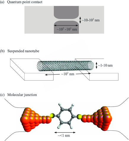
Figure 1: (Color online) Schematic representation of the different systems we consider in this Colloquium, ranging from metallic point contacts to molecular junctions.

In this Colloquium we will discuss all these issues at the microscopic level. The basic systems we will consider consist of a nanoscale junction, namely two leads connected by a nanoscale element, with possibly a third lead controlling some state variable of the system, e.g., its local temperature. Typical examples are point contacts or quantum dots placed between a two-dimensional electron gas van Houten et al. (1992a); Staring et al. (1993); Molenkamp et al. (1994); Godijn et al. (1999); Scheibner et al. (2007), a molecule trapped between a substrate and a scanning tunneling microscope (STM) tip Reddy et al. (2007); Baheti et al. (2008), metallic wires Ludoph and Ruitenbeek (1999), carbon nanotubes Kim et al. (2001); Yu et al. (2005) or silicon nanowires Hochbaum et al. (2007); Boukai et al. (2007) between two metal contacts, etc. Fig. 1 shows a schematic representation of the different systems we consider. The leads are held at different temperatures, which allow for the flow of energy (and possibly charge) through the junction. Here, we point out that, due to space limitations, we will not be able to discuss the entire class of systems collectively known as “nanomaterials” - composite layers of various materials fabricated on nanometer scales, which show unique electronic properties, often engineered by adding scattering mechanisms (for instance boundary scattering), that may be beneficial for energy applications Majumdar (2004); S. Volz (2009). The interested reader may refer to Chen Chen (2005) for systems other than those presented here.

To make the review easier to follow for the reader, we have divided it into three main (yet closely related) sub-topics. The first one is the transport of heat through the system by phonons (lattice vibrations) and electrons, which (in linear response) is mainly characterized by the thermal conductivity $\kappa$. This issue has already been reviewed elsewhere Galperin et al. (2007a); Wang et al. (2008), emphasizing the effects of vibrations and focusing primarily on the method of non-equilibrium Green’s functions. To make the present review complete, and in order to highlight the various theoretical methods and the open questions that still pertain to this subject, we give it some space here too. In particular, we will discuss the different processes that contribute to $\kappa$ and their importance in nanoscale junctions.

The second subject is that of the local temperature and heating inside the nanoscale system. This issue is particularly subtle, precisely because we are dealing with a non-equilibrium process where a temperature difference is set at the two sides of the nanojunction. We will address several experimental and theoretical issues and fundamental open questions, such as: How does one define a local temperature at the nanoscale in a non-equilibrium situation? What determines the local temperature and the temperature profile along the system?

As a corollary of the above studies we are finally led to analyze a nearly two-century old and important physical law, which so far has eluded a satisfactory theoretical understanding, namely Fourier’s law (FL). This law, as originally formulated, states that in the presence of a temperature difference between the two leads, (i) a temperature gradient develops, (ii) the energy current density is proportional to it, and (iii) the constant of proportionality is independent of system size. While FL was empirically postulated for bulk systems almost two centuries ago Fourier (1822) and has been derived phenomenologically for phonons more than eighty years ago Peierls (1929), no simple proof of its validity (or invalidity) has ever been derived from first principles, nor do we have a well-defined set of conditions to determine its validity for a given system Bonetto et al. (2000). As we will emphasize later, the issue has everything to do with the difficulty in defining the basic quantities that enter its formulation – namely the local temperature and heat current – from a microscopic, quantum mechanical point of view.

The final issue is that of the inter-relation between the heat flow and the electron transport through the junction, which can be collected under the general name of “thermoelectricity”. The central quantity here is the thermopower (or Seebeck coefficient) $S$, which describes the voltage drop generated by a temperature difference. A sample of important open questions for this topic are: What are the different mechanisms contributing to thermoelectricity? Are they properly taken into account in the present theories? What are the state-of-the-art experiments, and are their results interpreted satisfactorily?

All these issues and open questions will accompany us for the full length of this Colloquium. We will stress their importance for both their fundamental character as well as their impact in possible technological applications. We will finally point out possible future research directions that could explore them in more depth.

The Colloquium is organized as follows. In Sec. II we discuss heat flow in nanoscale systems due to phonons, electrons and their mutual interaction, and describe the different processes which contribute to it. We review both theoretical tools and state-of-the art experiments for measuring heat flow in nanostructures. We devote Sec. III to local temperature effects, and proceed to discussing Fourier’s law. In Sec. IV we discuss thermoelectric effects in nanoscale junctions. We give a detailed account of present theoretical tools, and discuss recent experiments, with emphasis on open issues in the field. Finally, we conclude in Sec. V with some prospects on the future of the field.

II Heat current and thermal conductivity

Let us start by reviewing the topic of heat current and thermal conductivity of nanoscale junctions. We will not present full derivations of the methods and results. Rather, we will outline only the main theoretical tools. The interested reader may find extensive accounts in recent reviews Galperin et al. (2007b); Wang et al. (2008); Dhar (2008) or books Akkermans and Montambaux (2007); Di Ventra (2008) where these methods are discussed in detail. In addition, we will review recent experimental advances in measurements of the thermal conductivity in nanoscale systems, with emphasis on the measurement process itself and open questions.

II.1 Definitions

When a nanoscale junction is placed in contact with leads held at different temperatures, energy flows through it. The original qualitative description for this phenomenon in bulk materials is attributed to Fourier Fourier (1822), and amounts to Fourier’s law which states that a temperature gradient $\nabla T$ induces a thermal current density linearly proportional to it, namely

$$j_{th}=-\kappa\nabla T~{}~{},$$ (1)

where $j_{th}$ is the heat current density (which may contain both phonon and electron contributions, see below) and $\kappa$ is the thermal conductivity (such an equation is usually valid only in the linear regime).

In Secs. III.2 and III.4 we will expand more on the significance of the term “temperature” for a system out of equilibrium, and its different definitions. Here, we anticipate that whenever we do not discuss its meaning explicitly we call temperature that which is measured by a local thermal probe weakly coupled to the system and whose temperature has been adjusted so that the system dynamics is minimally perturbed Di Ventra (2008). This defines what we will later call a temperature floating probe Dubi and Di Ventra (2009d); Dubi and Di Ventra (2009c). Note that we do not define it in terms of a probe adjusted so that the thermal current between the system and probe is zero, precisely because we do not have means to measure directly the thermal current (although these two definitions may give the same quantitative results). In addition, the reader needs to keep in mind that while this is an operational definition of temperature out of equilibrium, its actual experimental determination is far from trivial at present.

The validity of Eq. (1) in nanoscale junctions is discussed in detail in Sec. III.4. Here, we are mainly interested in the theoretical understanding and measurement of $j_{th}$ and $\kappa$, assuming that Fourier’s law is indeed valid. A relation between the formalism described below (Landauer’s formula (6)) and Fourier’s law can be determined, which requires calculation of thermal conductances at larger and larger length scales. Such derivation, discussed in other reviews Dhar (2008) implies going beyond the realm of nanoscale junctions and will thus not be discussed in detail here.

It is also convenient to introduce the thermal conductance, which is the ratio between the total heat current $J_{th}$ and temperature difference $\Delta T=T_{R}-T_{L}$,

$$\sigma_{th}=-\lim_{\Delta T\to 0}\frac{J_{th}}{\Delta T}~{}~{}.$$ (2)

If the sample is uniform with a constant cross section $A$ and length $L$, the thermal conductance is related to thermal conductivity $\kappa$ via $\sigma_{th}=\frac{A}{L}\kappa$. If the sample is not uniform, then the relation between thermal conductance and conductivity depends on the microscopic details of the system. In addition, in analogy with electric circuit theory, it is convenient to define the thermal resistance, being the reciprocal of the thermal conductance: $\rho_{th}=\sigma_{th}^{-1}$.

Energy can be carried through a nanoscale junction (or through a solid) either by lattice vibrations (phonons) or by electrons, or both . In insulating bulk materials the electronic contribution is negligible, while it is sizeable in bulk metals. This simple distinction is less obvious in nanoscale junctions, where, due to the large current densities they can carry, the two contributions may be equally important and need to be discussed on equal footing. For bulk insulating materials, the theory of phonon thermal conductivity based on the Boltzmann equation was derived by Peierls Peierls (1955) (see also the detailed review Carruthers (1961)). The main idea is that $\kappa$ is governed by phonon scattering, especially the so-called Umklapp scattering (processes that do not conserve crystal momentum), whereby phonons scatter between states which are separated (in reciprocal space) by a reciprocal lattice vector.  Considering a phonon mean-free path $l$ (mainly due to scattering by impurities), simple arguments lead to the following relation at high temperatures (in three dimensions) Ashcroft and Mermin (1976)

$$\kappa\approx\frac{1}{3}lvc_{v}~{}~{},$$ (3)

where $v$ is the velocity of sound and $c_{v}$ is the phonon heat capacity at constant volume (in the above equation optical and acoustic phonons are considered on equal footing, although only the latter ones participate in heat transport). In a bulk metal a similar relation can be derived Ashcroft and Mermin (1976), where now $l$ stands for the electronic mean-free path, $c_{v}$ is the electronic heat capacity at constant volume, and $v$ is the electron drift velocity. Here, a comment is in order. In the case of electrons the heat (or thermal) current contains also a contribution from the variation of number of particles. In fact, let us consider the thermodynamic relation (at constant volume) $\delta Q=d{\cal E}-\mu dn$, where $Q$ and ${\cal E}$ are the heat and energy per unit volume, respectively, $n$ is the particle number density, and $\mu$ the chemical potential. From this relation, dividing by the infinitesimal time interval $dt$, we obtain ($e$ is the electron charge)

$$J_{th}=J_{E}-\frac{\mu}{e}J_{e},$$ (4)

namely, for electrons the heat current has both a contribution from the energy current, $J_{E}$, and from the charge current $J_{e}$ (there is no such term for phonons, since their number is not conserved). In this review, we will use the terms “energy current” and “heat (thermal) current” interchangeably, but with the understanding that, in the case of electrons, one must generally include a contribution from the variation of the number of particles (see also discussion after Eq. (6)).

It is now natural to ask whether these arguments can be extended to the regime in which strong material inhomogeneities are the norm, like in nanoscale systems. Before we embark in this quest, however, it is worth asking why $\kappa$ is such an important quantity in the first place, especially since measuring the thermal conductivity at the nanoscale is all but trivial. The answer is that $\kappa$ contains information regarding two main processes relevant to the future applicability of nanoscale systems. The first is the rate at which energy is dissipated in and removed from the junction. This has an effect on the heating of the system, which may affect its structural stability. The second is that $\kappa$ is an important (and limiting) factor in the efficiency of nanoscale systems as heat-voltage converters (as it will be discussed more at length in Sec. IV). Therefore, according to the desired use, an ideal nanosystem should have opposite thermal properties: for current-carrying wires one wishes a high thermal conductance that would allow heat to pass through the wire and prevent over-heating, and for thermoelectric conversion one requires a thermal conductance as small as possible. These requirements make the understanding, predictability, and control of $\kappa$ highly desirable.

II.2 Experiment

In this section we focus on the experimental measurements of the thermal conductivity in nanoscale systems. As already pointed out, a major difficulty in measuring $\kappa$ (other than the usual ones related to any measurements at the nanoscale) stems from the simple fact that there is no direct way to measure a heat current. Indeed, the only directly measurable quantities are electrical currents, voltages and temperatures (the latter also typically measured via resistance measurements), and from these one deduces $\kappa$. The main limitation is that the value of $\kappa$ as extracted from the experiment may then depend on the model used to describe the whole experimental setup or device, which may generate some ambiguity. Here, we will describe some recent experiments, discuss the methods employed in deducing $\kappa$, and review some of the main results.

A conceptually simple way to measure the thermal conductance of a suspended nanojunction is the following. Consider the schematic system of Fig. 2. The “heater” coil is heated by passing a current through it. By measuring the current and the voltage through the heater coil, the power transferred through it is given by the well-known relation, $P=IV$. This power increases the temperature of the coil to $T_{h}$. At the same time, the temperature of the “sensor” coil, $T_{s}$, is evaluated (by measuring its resistance, which is pre-calibrated to correspond to a given temperature). If the wire is suspended, then the entire heat current should be equal to the power supplied by the heater coil, $\dot{Q}=P$, which is related, in linear response, to the temperature difference by

$$\dot{Q}=-\sigma_{th}(T_{h}-T_{s})\;,$$ (5)

from which the thermal conductance $\sigma_{th}$ can be evaluated, under the assumption that all the power supplied by the electric circuit flows through the junction without loss, and the thermal conductivity $\kappa$ can then be extracted from a microscopic model that relates thermal conductivity to thermal conductance (see Sec. II.3). If, as indeed is the case in many experiment, some of the power is lost due to heat diffusion away from the contacts (e.g. into the substrate) then the Joule heating is the sum of the heat flowing away through the contacts and that flowing through the wire.

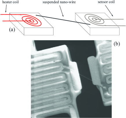
Figure 2: (Color online) (a) A schematic representation for a simple setup to measure the thermal conductance. (b) An actual device to measure the thermal conductance of boron nitrade nanotubes (from Chang et al. (2006)).

This method seems very simple, and was indeed employed to measure the quantum of thermal conductance Schwab et al. (2000). However, it needs to be acknowledged that it has obvious limitations. For one, dissipative effects at surfaces or local thermal gradients in the heating and cooling parts of the coils  may reduce the heat flow in the suspended wire. In addition, recent theoretical studies indicate that the contact thermal resistance between nanowires and substrate plays an important role in determining the overall thermal resistance Zhong and Lukes (2006); Chalopin et al. (2008).

More difficult is the determination of the thermal conductivity $\kappa$ from a model that includes all the effects of device geometry and dissipation through the contacts and substrates. Such models vary for different devices and geometries Shi et al. (2003); Chang et al. (2006, 2008), but share the common feature that thermal conductances are treated on the same footing as classical (charge) conductances, with the same Kirchhoff-like laws for the addition of resistances in series ($\rho_{th}=\sum_{i}\rho_{th,i}$, with $\rho_{th,i}$ the thermal resistance of a single element of the circuit) and parallel ($\rho_{th}^{-1}=\sum_{i}\rho_{th,i}^{-1}$). Thus, the measured thermal conductivity may depend on the circuit model used, which makes it hard to compare between different experiments. This means that when performing a measurement, one is in fact measuring the thermal conductance of the system of interest embedded in that specific device. Nevertheless, this method was used to study the thermal conductivity of many nanoscale structures, mainly carbon nanotubes Brown et al. (2005); Chang et al. (2006, 2008); Shi et al. (2003); Chiu et al. (2005); Fujii et al. (2005); Kim et al. (2001); Yu et al. (2005) but also nanotubes of other materials Chen et al. (2008); Chang et al. (2008); Li et al. (2003). Some experimental features are universal, like ballistic thermal conductance Brown et al. (2005); Chiu et al. (2005), a value of $\kappa$ which is orders of magnitude larger than the bulk value for carbon nanotubes ($\sim 3000W/K$ at room temperature), an increase of thermal conductance with nanowire diameter, or a peak of the thermal conductance at $\sim 320K$ Fujii et al. (2005); Kim et al. (2001), attributed to the onset of Umklapp phonon scattering processes. However, other features, such as the detailed power-law dependence of $\kappa$ on temperature vary between experiments, indicating that this is not a universal feature, and depends on the details of the experimental setup.

Other experimental approaches to measure $\kappa$ have been introduced in the literature. For instance, Pop et al. Pop et al. (2006) have used high currents to induce heating in a single-walled carbon nanotube, with a model to relate the current-voltage (I-V) characteristics to the high-temperature thermal conductance. In another example, the so-called $3\omega$ method Cahill (1990); Lu et al. (2001), was used to study nanotubes Bourgeois et al. (2007); Choi et al. (2005, 2006). In this method, an a.c. current is applied to the sample which also acts as a heater. From a simple derivation one finds that the third harmonic of the voltage drop across the sample is related to the thermal conductivity of the sample (at small frequencies of the current). Using this method, the authors found a deviation of the thermal conductance from a cubic dependence on temperature for Si nanowires, indicating a dimensional crossover at low temperatures. Both these methods rely on current-induced self-heating of the sample (rather than direct heating by an external source). In a third example, laser-induced heating and Raman spectroscopy (already used in various nanoscale systems such as graphene ribbons Balandin et al. (2008); Calizo et al. (2007)) have been used to determine the local temperatures Hsu et al. (2009); Deshpande et al. (2009) and extract the thermal conductance of carbon nanotube bundles. The main disadvantage of this method is that to obtain the thermal conductance one needs to assume a value for the optical absorbtion of the sample, which is usually unknown.

II.3 Theoretical Methods

We now provide a brief description of the theoretical methods most commonly employed to describe energy flow, with an eye on their strengths and limitations.

II.3.1 Single-particle scattering approach

Many theoretical calculations of thermal conductance are based on an approach pioneered by Landauer Landauer (1970, 1957) in the context of charge transport in mesoscopic and nanoscopic systems Imry (1997); Di Ventra (2008); Datta (1997). The same ideas have been generalized to phonon transport through a nanoscale junction Dhar and Roy (2006); Angelescu et al. (1998); Rego and Kirczenow (1998); Rego (2001); Blencowe (1999, 2004); Segal et al. (2003).

The basic tenet of this approach is that one assumes the leads non-interacting (otherwise no closed form for the current can be obtained Di Ventra (2008)), so that a convenient basis, such as plane-waves, can be chosen to develop state vectors for both types of particles, either phonons or electrons. As a further conceptual simplification, the leads are thought to be adiabatically “connected” to reservoirs whose only role is to define the occupation of the scattering states according to a local equilibrium Bose-Einstein (BE) distribution for phonons or a Fermi-Dirac (FD) distribution for electrons. Once this occupation is set, the particles are free to propagate in the leads before scattering at the lead-system interface. Charge and/or energy current is then determined by an electrochemical potential difference and/or a temperature difference between the reservoirs.

Most of the calculations also assume that the particles in the sample are either truly non-interacting or interacting at a mean-field level (which is the same from a formal point of view). In this case the current is simply proportional to the probability for the particles to cross the sample from one electrode to the other. For instance, in the case of phonon transport, phonon states at a given energy $\hbar\omega$, scatter off the junction and may be either transmitted through it or reflected back. The probability to be transmitted through the junction is characterized by the transmission coefficient ${\cal T}(\omega)$. The expression for the heat current is then simply

$$J_{th}=\int^{\infty}_{0}\frac{d\omega}{2\pi}\hbar\omega{\cal T}(\omega)(g_{L}-g_{R})~{}~{},$$ (6)

where $g_{L(R)}=1/\left(\exp\left(\frac{\hbar\omega}{k_{B}T_{L(R)}}\right)-1\right)$ are the distribution functions of phonons in the left (right) lead. From $J_{th}$ one can then evaluate the thermal conductance according to Eq. (2).

Within this approach the electronic contribution to the heat current is calculated similarly, where in Eq. (6) one makes two changes, namely (i) the BE distribution functions are replaced by FD distributions, and (ii) the energy in each reservoir is measured from the respective electrochemical potential, $\mu_{L}$ and $\mu_{R}$ for the left and right reservoir, respectively, i.e., $\hbar\omega\rightarrow\hbar\omega-\mu_{L,R}$ (see Eq. (4)). In linear response this leads to the substitution $\hbar\omega\rightarrow\hbar\omega-(\mu_{L}+\mu_{R})/2$ in the energy term that multiplies ${\cal T}(\omega)$ in Eq. (6).

To actually evaluate $\sigma_{th}$, one has to compute the transmission coefficient ${\cal T}(\omega)$. To this aim several methods have been employed, such as the use of continuum models Angelescu et al. (1998), boundary condition method Wang and Wang (2006), mode-matching method Khomyakov and Brocks (2004); Ando (1991); Ting et al. (1992) and scattering or transfer matrices Tong et al. (1999); Di Ventra and Lang (2002). All these methods are fundamentally equivalent, and in fact have their origin in the single-particle elastic scattering theory of conduction (see, e.g., Di Ventra (2008)), whereby one can write the transmission coefficient as a sum of all the partial probabilities of transmission $T_{if}(\omega)$ from one of the momentum states of the incoming ($i$) particle (whether electron or phonon) at energy $\hbar\omega$ to one of the momentum states of the outgoing ($f$) particle at the same energy, namely Büttiker et al. (1985)

$${\cal T}(\omega)=\sum_{i}\sum_{f}T_{if}(\omega)=\mathrm{Tr}\{\tau\tau^{\dagger}\},$$ (7)

where $\tau$ is a sub-matrix of the scattering matrix with dimensions $N_{R}\times N_{L}$, with $N_{R}$ and $N_{L}$ the number of channels in the right and left leads, respectively, at energy $\hbar\omega$. This result can be cast in another equivalent form in terms of single-particle Green’s functions via Meir and Wingreen (1992)

$${\cal T}(\omega)=\mathrm{Tr}\left\{G^{r}\Gamma_{L}G^{a}\Gamma_{R}\right\},$$ (8)

where $G^{r(a)}$ is the retarded (advanced) single-particle Green’s function corresponding to the interaction of a “central” part of the junction with the electrodes and $\Gamma_{L(R)}$ describe the “rate” at which particles scatter between the leads and the central part of the junction. It has been re-derived for thermal transport by many authors Ozpineci and Ciraci (2001); Segal et al. (2003); Wang et al. (2006); Mingo and Yang (2003); Mingo (2006); Yamamoto and Watanabe (2006); Galperin et al. (2007a); Wang et al. (2007); Dhar (2008).

Arguably the most universal result obtained from the Landauer formula (6) is that of thermal conductance quantization. Similarly to the quantization of electrical conductance in ideally one-dimensional (1D) electronic systems van Wees et al. (1988), at low temperatures the thermal conductance (per phonon mode) was predicted to acquire a quantized value

$$\sigma_{0}=\frac{\pi^{2}k^{2}_{B}T}{3h}~{}~{},$$ (9)

where $h$ is Planck’s constant Pendry (1983); Maynard and Akkermans (1985); Greiner et al. (1997); Rego and Kirczenow (1998). This result is readily derived from Eq. 6 in linear response by setting the number of modes to unity, and letting the transmission coefficient to be one, i.e., ${\cal T}(\omega)=1$.

The fact that this conductance is material-independent relies on the fact that, like in the electronic case, in 1D the phonon density of states is exactly proportional to the inverse of the group velocity. Remarkably, thermal conductance quantization does not depend on the statistics of the carriers Rego (2001). Indeed, $\sigma_{0}$ was experimentally measured for phonons Schwab et al. (2000), electrons Nicholls and Chiatti (2008); Chiatti et al. (2006) and even photons Meschke et al. (2006).

Another application of the Landauer formula (6) has been in the study of geometrical and temperature effects on thermal transport. To give a few examples, this approach has been used to understand the role of defects on the thermal conductance of a nanowire Chen et al. (2005a), the effects of different geometries such as stubs, T-junctions and concavities Peng et al. (2007); Tang et al. (2006); Xie et al. (2008), periodic modulations Tang et al. (2007), and surface roughness Kambili et al. (1999); Santamore and Cross (2001). As a general rule, disorder and temperature are found to have competing roles: disorder tends to reduce the thermal conductance (by decreasing the transmission coefficients of the different transport modes), and a temperature increase usually results in a larger thermal conductance, due to an increased number of modes which participate in the thermal transport.

The interplay between the two processes can result in interesting phenomena. For instance, Santamore et al. Santamore and Cross (2001) showed that disorder in the form of surface roughness may generate a non-monotonicity in $\sigma_{th}$ with increasing temperature, with a slight decrease (below the quantum of thermal conductance) followed by a rise of $\sigma_{th}$ with increasing temperature, in similarity to the experimental results of Schwab et al. Schwab et al. (2000). Their results (shown in Fig. 3) are explained as follows: at very low temperatures, there is only one mode which contributes to the thermal conductance. As temperature increases, scattering of that mode off the surface roughness increases, generating a decrease in the thermal conductance. As the temperature is raised even higher, higher modes start to participate in the thermal transport, giving rise to an increase in the thermal conductance.

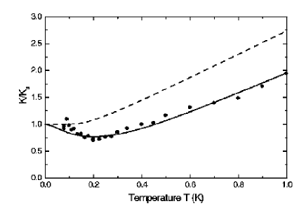
Figure 3: Thermal conductance of a quasi-1D wire with surface roughness, exhibiting inhomogeneous thermal conductance. Points correspond to experimental data of Schwab et al.Schwab et al. (2000), and the solid line is the theoretical curve. From Santamore and Cross (2001).

This ties with the use of the scattering approach to thermal conduction in real materials, which comes about from using realistic phonon spectra (e.g., as obtained from experiment or first-principles approaches) in combination with ground-state density-functional theory (DFT) calculations to obtain the scattering coefficient ${\cal T}(\omega)$. To give several examples, Tanaka et al. have combined geometrical structure (i.e., realistic shape of the wire) with real material parameters to study the onset of the thermal conductance quantization in GaAs and silicon nitride wires Tanaka et al. (2005). The thermal conductance of nanowires made of, e.g., Si, Ge and GaAs was studied by several authors Tanaka et al. (2005); Mingo and Yang (2003); Mingo et al. (2003); Wang and Wang (2007). Much attention has been given to carbon-based structures, such as carbon nanotubes, graphene and graphite Zhang and Li (2005); Mingo and Broido (2005a, b); Yamamoto et al. (2004); Yamamoto and Watanabe (2006); Zimmermann et al. (2008); Lan et al. (2009); Lü and Wang (2008). Another example is the recent study of isotope and disorder effects Murphy and Moore (2007), specifically in carbon and boron-nitride nanotubes Stewart et al. (2009); Savić et al. (2008a, b).

Some universal conclusions arise from these calculations. For instance, a dimensional crossover from three- to one-dimensional transport (manifested by, e.g. a change in the temperature dependence of the thermal conductance) occurs in many systems as the diameter of the nanotube decreases, the length scales determined by the wavelengths of the typical phonon modes Wang and Wang (2007). Also, disorder in various forms (local defects, surface roughness, etc.) has a dramatic effect on the thermal conductance, as it influences the scattering of the different modes Roy and Dhar (2008). Due to the translational invariance of the lattice, long wavelength (or zero-frequency) modes are always conducting, while short wavelength modes are scattered by disorder. Since the short wavelength modes participate in the thermal transport only at high temperatures, it is found that the low-temperature thermal conductance is less affected by disorder and defects. Finally, the thermal conductance of molecular junctions has also been widely studied Segal et al. (2003); Galperin et al. (2007a); Mingo (2006). It is found to be strongly dependent on a multitude of factors, among which the phonon spectrum of the molecules, the degree of localization of the molecular modes, the molecule-lead coupling, non-harmonicity (i.e. phonon interactions), etc.

It is important to stress once more that Eqs. (6), (7),  (8), and indeed the whole Landauer approach, are based on some strong assumptions, which may breakdown in nanoscale junctions and under certain experimental conditions. The first assumption is that the system is “closed”, in the sense that it does not dynamically interact with its environment. The latter only provides the boundary conditions and the relevant parameters (like the temperatures, chemical potentials, etc.). The second assumption is that the leads are ideal, i.e., are unaffected by the proximity to the junction (either in their structure or in the distribution of particles) and support well-defined single-particle states. In addition, it is assumed that “dissipation” takes place at the (infinitely far) edges of the leads and that the temperature (and chemical potential for electrons) is uniform in them. Most critically, the approach does not provide information on the dynamics of the system. Therefore, transient, memory and non-linear dynamical phenomena are beyond its reach. A further issue arises when one uses ground-state DFT in combination with the Landauer approach: one is effectively using a ground-state theory for a non-equilibrium problem. This issue cannot be solved by knowledge of the exact ground-state exchange-correlation functional, and as such, the use of ground-state DFT in this context can only be viewed as a mean-field approximation. This has been explicitly demonstrated in Vignale and Di Ventra (2009), where for the case of electrical conductance it was shown that the exact resistivity tensor $\stackrel{{\scriptstyle\leftrightarrow}}{{\rho}}$ can be written as

$$\stackrel{{\scriptstyle\leftrightarrow}}{{\rho}}=\stackrel{{\scriptstyle\leftrightarrow}}{{\rho}}_{s}+\stackrel{{\scriptstyle\leftrightarrow}}{{\rho}}_{xc}$$ (10)

where $\stackrel{{\scriptstyle\leftrightarrow}}{{\rho}}_{s}$ is is the resistivity tensor of a noninteracting system in the presence of a static potential $V_{s}$ that reproduces the exact ground-state density, and $\stackrel{{\scriptstyle\leftrightarrow}}{{\rho}}_{xc}$ is a dynamical contribution related to dynamical exchange-correlation effects, and which does not vanish even in the zero-frequency (d.c.) limit. A possible way out would be to use a fully dynamical approach (e.g., the microcanonical picture of transport as suggested in Di Ventra and Todorov (2004)) combined with time-dependent DFT Runge and Gross (1984). This approach (recently implemented to study charge transport Cheng et al. (2006)) would provide, in principle, the exact thermal total current, if the exact dynamical exchange-correlation potential is known. However, we are not aware of any calculation of thermal current along these lines.

II.3.2 The role of interactions

Up to this point the system Hamiltonian has been assumed to describe single particles with interactions included at most at the mean-field level. As briefly mentioned above, many-body correlations can be accounted for within a time-dependent DFT approach, namely within an effective single-particle picture. Alternatively, the effect of interactions beyond mean-field, could be explicitly included via the so-called non-equilibrium Green’s functions formalism (NEGF) (see, e.g., N. Mingo, chapter $3$ in S. Volz (2009)). In this approach one solves equations of motion for appropriate single-particle Green’s functions that can be conveniently defined on the Keldysh contour Kadanoff and Baym (1962); Keldysh (1964). In its exact formulation, the NEGF has however limited practical utility, since if one assumes particles interacting - beyond mean-field - in the whole system (leads plus nanostructure) no closed equation of motion for the single-particle Green’s functions can be obtained Di Ventra (2008). Instead, it is common to assume (as in the Landauer approach) that the leads contain non-interacting particles and interactions are confined within a “central” region containing the nanostructure. This is a strong assumption and may not always correspond to the physical problem at hand and/or its experimental realization.

If one makes the assumption of non-interacting particles in the leads, and assumes that a steady-state has been reached in the long-time limit (not an obvious statement either), the equation of motion for the different single-particle Green’s functions can be closed and the NEGF provides a compact expression for the total current similar to that derived for electron transport Meir and Wingreen (1992), given by

$$J = \frac{1}{4\pi}\int^{\infty}_{0}\hbar\omega d\omega\left[(G^{r}-G^{a})(\Sigma^{<}_{R}-\Sigma^{<}_{L})+\right.$$ (11)

$$~{}~{}~{}~{}~{}~{}~{}~{}\left.+iG^{<}(\Gamma_{R}-\Gamma_{L})\right]~{}~{},$$

where $G^{r,a,<}$ are the retarded, advanced and “lesser” single-particle Green’s functions, respectively; $\Sigma^{<}_{\alpha}$ are the “lesser” self energies of the $\alpha=L,R$ leads and $\Gamma_{\alpha}=i(\Sigma^{r}_{\alpha}-\Sigma^{a}_{\alpha})$ namely the difference between “retarded” and “advanced” self energies (the explicit $\omega$-dependence of all these quantities has been omitted). The first term on the right hand side of Eq. (11) may be interpreted as describing the current from the bias-induced difference in the coupling to the leads, while the second is related to the non-equilibrium distribution function in the interacting region. The single-particle Green’s functions can represent either phonons or electrons, and should be calculated in the presence of interactions. In the mean-field approximation, Eq. (11) reduces to Eq. (6) (or its equivalent form for fermions). Many-body perturbation expansions to compute these Green’s functions have been performed for simple model Hamiltonians Galperin et al. (2007a); Lü and Wang (2007) but it is no easy task to introduce interactions (beyond mean field) in realistic systems.

The NEGF could also be used to study the effects of electron-phonon interactions. In that case as well, however, quite strong approximations need to be made in order to have an analytically tractable theory. For instance, if one assumes electrons interacting with each other at a mean-field level, but interacting in a “central” region with non-interacting phonons, the heat current can be approximated as a sum of contributions from both electrons and phonons, $J=J_{el}+J_{ph}$ , each component calculated with the help of Eq.  (11). The key ingredient here is that, due to the electron-phonon interaction, the self-energy of phonons includes an electronic contribution and vice versa. These contributions can be calculated in a perturbative way. However, this is clearly an idealization, since it neglects correlated electron-ion motion, which, in principle, does not even allow the total thermal current $J$ to be separated into two distinct contributions from the two particle species. Along the same lines of reasoning, the effects of phonon-phonon interaction have been studied Xu et al. (2008); Liu and Yi (2006); Mingo (2006). According to these results both electron-phonon and phonon-phonon interactions decrease the thermal conductivity. However, we need to stress once more that due to the large current densities nanoscale systems carry - and hence the large number of scattering events per unit time and unit volume - it is not a simple task to include all the relevant physical scattering mechanisms in the present non-equilibrium case. An example of this is the possibility of phonon modes in the junction which are weakly coupled to the bulk modes of the electrodes. In this case, these “localized” modes may be energetically “pumped” by scattering with electrons or other phonons before energy could efficiently be dissipated away. This physical situation is beyond second-order perturbation theory and more work in this direction is thus highly desirable.

II.3.3 Molecular dynamics

Another method to evaluate the thermal conductivity which is gaining increasing popularity is that of molecular dynamics (MD). Basically, molecular dynamics comes down to solving the classical equations of motion of the system numerically. The origin of the method in the present context can be traced back to the seminal work of Fermi, Pasta and Ulam Fermi et al. (1955), where the energy transfer in non-harmonic lattices has been studied numerically. Since then it has been widely used to study heat transport in classical 1D systems Dhar (2008); Lepri et al. (2003). It has also been generalized to study quantum effects, by providing appropriate boundary conditions Wang et al. (2008). These approximations, however, should be thought of as quasi-classical, since the microscopic dynamics of the system is described by classical Newtonian equations of motion, and the quantum nature is only introduced via indirect conditions (such as the noise in a Langevin term). A big advantage of molecular dynamics is the ability to model realistic systems and geometries in a rather straightforward way. The forces between atoms are evaluated from realistic parameters, so that different geometries, impurities, structures, etc. are easily taken into account.

In order to calculate the heat transport directly from MD, one needs to account for a finite temperature in the system. This is usually done in linear response by adding to the Newtonian equations of motion a Langevin fluctuating term which satisfies the fluctuation-dissipation relation, i.e., the two-time correlation function of the current is proportional to the temperature (see, e.g., Van Kampen (2001)). Alternatively, a Nosé-Hoover thermostat is introduced, in which a fictitious coordinate is added to the real coordinate to maintain a finite temperature Nosé (1984); Hoover (1985).

Once a finite temperature is set, there are two main methods to calculate the thermal conductivity. The first (sometimes called equilibrium MD) is via the linear-response Green-Kubo formula Luttinger (1964); Dhar (2008); Lepri et al. (2003)

$$\kappa=\frac{1}{3Vk_{B}T^{2}}\int^{\infty}_{0}\langle J_{th}(t)J_{th}(0)\rangle dt~{}~{},$$ (12)

where $V$ is the volume, $k_{B}$ the Boltzmann constant, $T$ is the system temperature, $J_{th}(t)=\int d{\bf r}j_{th}({\bf r},t)$ is the integral of the heat current density, $j_{th}({\bf r},t)$, over the entire system, and the brackets denote equilibrium ensemble averaging in the absence of a thermal gradient. However, the Green-Kubo equation has two main weaknesses. The first is that it is derived in the thermodynamic limit and therefore its use in finite systems is not well justified Kundu et al. (2009). Secondly, one needs to assume that a small temperature gradient (the external perturbation) ensues in the system, which may not be the case in every experiment. However, its relative simplicity makes it a good starting point in many cases.

An alternative method (also known as nonequilibrium MD), still based on molecular dynamics, is the one in which the system is held in contact between two heat baths of different temperatures. Once the dynamics reaches a steady state, the temperature profile and the local heat currents can be calculated, from which the thermal conductivity is extracted. Here lies one of the disadvantages of the model, since the definition of the local heat current requires defining a local energy operator, which is not always a unique quantity Lepri et al. (2003); Wu and Segal (2009). Likewise, a local temperature needs to be defined and evaluated; a somewhat tricky issue to which we will come back in Sec. III. At high temperatures (where the distribution function is practically classical and quantum effects are negligible; say at temperatures higher than the typical vibrational mode temperature) one may define the local temperature as the kinetic energy of the atoms (via the equipartition function), but this assumption breaks down at low temperatures, and one needs to use a definition of temperature which rests on the equilibrium distribution of phonons Wang et al. (2008). This yields a quasi-classical treatment (which is somewhat better than a fully classical treatment at low temperatures), but leans on the assumption that the phonon distribution resembles its equilibrium form, which may not be the case in this non-equilibrium problem. On the other hand, the obvious advantage of this method is that it does not rely on any thermodynamic-limit assumptions and is thus applicable for any system size, which is important for the study of realistic nanoscale systems. For instance, Yang et al. Yang et al. (2010) recently used the method to study Fourier’s law and thermal conductance of realistic Si nanowires, and showed that Fourier’s law breaks down in these systems (see Sec. III.4). Studies along similar lines have been recently performed to investigate the thermal conductance of carbon nanotubes Berber et al. (2000); Hu et al. (2008); Padgett and Brenner (2004), Si wires Ponomareva et al. (2007); Yang et al. (2008); Henry and Chen (2008b), diamond nano-rods Padgett et al. (2006) and polyethylene chains Henry and Chen (2008a), to name only a few recent studies.

An additional method, related to MD, is that of lattice dynamics models. In this method the phonon dispersion relations are obtained by calculating the direct change in energy due to atom displacements, using force fields obtained from DFT calculations Ren et al. (2006); Feldman et al. (2000); Turney et al. (2009).

The abundance of literature makes it hard to describe universal features of the thermal conductance, which seems to strongly depend on the details of the model and/or material. Specifically, $\sigma_{th}$ is very sensitive to the phonon spectra and to phonon localization Dhar and Lebowitz (2008); Zhernov and Chulkin (2000), which are in turn sensitive to material, geometry and disorder, surface roughness, and more. The rationale behind these studies is that by uncovering the detailed influence of these parameters on $\sigma_{th}$, theory may provide guidance to experiments and even suggest new materials with optimized thermal properties.

III Local temperature and heating

III.1 General remarks

When a current passes through a classical resistor, the latter heats up. This phenomenon is known as “Joule heating”. It is a consequence of the inelastic relaxation of electrons in the resistor which transfer energy to the surrounding lattice Ashcroft and Mermin (1976). In a nanoscale system, such as a molecular junction or an atomic wire, electrons can analogously scatter inelastically off the phonons (i.e., the vibrational modes of the structure). However, since electrons typically spend very little time in the junction region, one might naively think that their inelastic scattering rate is negligible with consequent little heating of the junction itself. This conclusion, which is, for instance, at the heart of the Landauer scattering approach where all dissipation is assumed to occur only in the “reservoirs”, does not take into account the fact that due to the small cross-section of nanoscale systems, the current density at the junction can be very large (typically much larger than in mesoscopic and macroscopic systems, see footnote 3). This implies that the power per atom in the junction can be very large, possibly leading to large local heating Todorov (1998); Chen et al. (2003); Chen et al. (2005b). The rate at which this power is then dissipated back to the electrodes determines the effective local (and out of equilibrium) temperature of the junction.

In addition, current-carrying electrons can transfer energy, via inelastic electron-electron interactions, to other electrons in the Fermi gas D’Agosta et al. (2006). This effect is generally small in macroscopic systems. However, similarly to the increased rate of electron-phonon scattering in nanoscale junctions due to the large current densities, the inelastic scattering rate of electron-electron interactions may increase in nanoscale systems leading to a local heating of the electron liquid D’Agosta et al. (2006). This effective higher temperature of the electrons may influence the local ionic heating due to electron-phonon interactions and thus can be indirectly measured, by measuring the local temperature of the ions or the broadening of inelastic conductance features D’Agosta and Di Ventra (2008a).

An obvious reason why local temperatures and heating are such important phenomena lies in the fact that substantial heating of a nanoscale system leads to the system instability and eventually to the breaking of atomic bonds Teramae et al. (2008); Tsutsui et al. (2008b); Ward et al. (2008). A different and even more fundamental interest in these phenomena arises in the context of Fourier’s law, Eq. (1), that we will discuss in Sec. III.4. Of course, at the nanoscale, it seems inappropriate to discuss the scaling of the thermal conductance with length, since this is an asymptotic (in terms of system size) property Lepri et al. (2003). Thus, one is left with the simple question: under which physical conditions does a uniform temperature gradient develops in a nanoscale system held in contact between two heat baths of different temperatures?

In this section we discuss all these issues. We review the various mechanisms which give rise to heating in current-carrying junctions, using simple arguments and models, followed by some basic results obtained from more elaborate models. We then turn to discuss the onset of a temperature gradient, analyzing a molecular wire junction in terms of the theory of open quantum systems, discussed in some detail in Sec. IV.3.2.

III.2 Heating in current-carrying nanostructures: theory

III.2.1 Various definitions of out-of-equilibrium temperature

In order to discuss local heating, the first question one should ask is: how is a local temperature defined and calculated? Since temperature is a thermodynamic quantity, some caution is needed Hartmann et al. (2004a); Hartmann and Mahler (2005); Hartmann et al. (2004b). Apart from the definition of temperature that we have given in Sec. II.1, and which we will use also in Sec. III.4, we here report several other notions of local temperature (not necessarily leading to the same quantitative results) and their microscopic origin, which were used to study local ionic heating in atomic junctions, each with its own pros and cons.

Kinetic definition - An intuitive definition of local temperature is to relate it to the local kinetic energy of the ions, i.e. $\langle{\scriptstyle 1\over 2}mv^{2}\rangle\sim 3k_{B}T/2$. However, this definition, mainly used in molecular dynamics simulations (see Sec. II.3.3), has several drawbacks: (i) it relies on the equipartition theorem which is strictly proven in the thermodynamic limit only for systems whose energy is quadratic in the particle momenta (as for non-interacting systems), and does not encompass any quantum effects. (ii) One needs to define an average kinetic energy over some length scale, while the quantum nature of particles may preclude such definition.

Local phonon mode - Consider a phonon mode somehow coupled to the system and vary its temperature in such a way that no heat flows between that mode and the system. This idea is somewhat similar to the idea of connecting an external bath to a system and imposing that no heat current flows between the system and bath, which was suggested to study the onset of Fourier’s law in one-dimensional systems, both classical and quantum Bonetto et al. (2004); Dhar (2008); Dhar and Roy (2006); Roy (2008). This idea was recently used to study the local temperature of a model molecular junction using the NEGF formalism Galperin et al. (2007a, b). The main result is the existence of two voltage thresholds. The first is at the voltage which corresponds to the vibrational energy of the phonon, $eV\sim\hbar\omega_{0}$, at which local heating starts to occur and the temperature increases abruptly. The local temperature then remains roughly constant, until it rises again when the bias is so large as to encompass the molecular conduction window (i.e., both the HOMO and LUMO states). The disadvantage of this method is that the temperature of the mode depends on the microscopic details, i.e., the phonon excitation energy $\hbar\omega_{0}$ and/or the electron-phonon coupling.

Distribution function definition - A slightly different model of local temperature is to connect a phonon mode to the nanoscale system, but instead of determining its temperature self-consistently, its distribution function is compared to an equilibrium distribution function with a given temperature, which is tuned to give the best comparison. Clearly, the disadvantage of this method is that the non-equilibrium distribution function may be very different from the equilibrium one Pekola et al. (2004); Koch et al. (2006). The last two methods were compared, and were found to give similar local temperatures at large bias (compared to the typical vibrational modes, implying strong non-equilibrium and population of higher modes), but deviated from each other substantially at low biases. In fact, the second method turned out to give erroneous results in the zero-bias limit, when one expects the temperature to be the same as that of the leads. This is precisely because an equilibrium form for the phonon mode was assumed, although even with no current the distribution function of the mode may have contributions arising from the coupling to the electronic (and other phononic) degrees of freedom in the junction Galperin et al. (2007a).

Definition from dissipated power - A microscopic theory which relies on first-principles was suggested by Chen and coauthors Chen et al. (2003); Chen et al. (2005b). The method is as follows. As a starting point, the electronic scattering states are calculated using ground-state DFT. The electron-phonon coupling for the different modes is also calculated using first-principles approaches. Using perturbation theory then one can calculate the power dissipated into the junction from current-carrying states. This power is then compared to the rate at which heat escapes the junction, typically assumed as $\sigma_{th}T^{4}$ with $\sigma_{th}$ the thermal coefficient that can be estimated from a microscopic model, and $T$ the effective temperature of the junction Chen et al. (2003); Chen et al. (2005b). A result of these calculations is presented in Fig. 4, where the local temperature as a function of bias was calculated for a benzene-dithiol (BDT) junction and a gold-atom point contact. The results indicate that, for a given bias, the BDT junction heats up less than the gold-atom junction, due to better thermal coupling with the electrodes and larger resistance to electrical currents (see Eq. 13). This result is also confirmed by experiments on similar systems Tsutsui et al. (2007); Teramae et al. (2008); Huang et al. (2006). While not visible from Fig. 4, theoretical results of the threshold voltage for heating - see Eq. 13 - are also in good agreement with experiments Chen et al. (2003); Chen et al. (2005b). The same method was used to study local heating in alkane chains of different lengths Chen et al. (2005b). It was predicted that, at fixed voltage, heating decreases with increasing chain length, which is due to increased resistance to electron flow; a result also confirmed experimentally Huang et al. (2007). More recently, the same approach was used to study the effect of different isotope substitutions on the heating in hydrogen molecular junctions Chen (2008). It was found that local heating is very sensitive to isotope effects since the electron-phonon coupling constant is inversely proportional to the ionic mass.

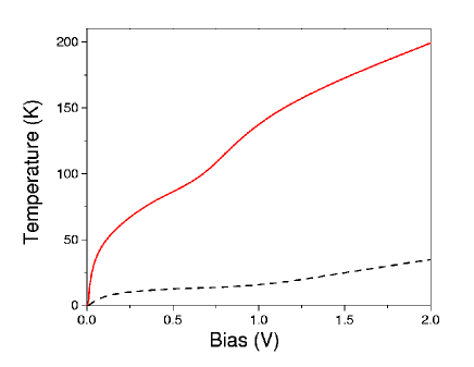
Figure 4: (Color online) Local temperature as a function of bias, calculated from a scattering theory approach, for a benzene-dithiol molecular junction (dashed line) and a gold-atom point contact (solid line). From Chen et al. (2003).

The method described above has the advantage that it can treat realistic systems. However, its main drawback is that it relies on the assumptions of the Landauer approach - see Sec. IV.3.1 - and its practical implementation employs ground-state DFT, which, as we have discussed at length in this review, does not take into account properly all dynamical effects.

III.2.2 Ionic heating

After discussing various definitions of local temperature, we are now in a position to discuss local heating. As described previously, we consider here a junction, composed of leads (which are assumed to be held at local equilibrium), and a nanoscale system which has both electronic and vibrational degrees of freedom. Even in the presence of current, we can assume that in the leads, far away from the nanojunction, electrons and phonons reach the same temperature $T_{0}$ . In the junction, however, the electrons and phonons may have different temperatures, $T_{e}$ and $T_{ph}$, respectively. These temperatures depend on bias, strength of electron-phonon and electron-electron interactions, the coupling of phonons with the bulk phonons in the leads, as well as the transmission properties of the electrons.

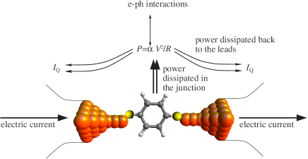
Figure 5: (Color online) A schematic representation of the mechanism of ionic heating in nanoscale junctions. The electric current dissipates a fraction $\alpha V^{2}/R$ of its power in the junction, depending on the strength of the electron-phonon interaction. This power is then dissipated to the phonons in the electrodes in the form of a heat current. The balance between the power flowing into the junction and the heat current $I_{Q}$ flowing out of the junction determines the ionic temperature of the junction.

Let us start by discussing the temperature of the ions in the junction, or the phenomenon of local ionic heating (see schematic in Fig. 5). We start from some simple considerations assuming first no inelastic electron-electron scattering occurs Todorov (1998); Di Ventra (2008). The power of the entire circuit (nanojunction plus power source) is given by $V^{2}/R$, where $V$ is the source bias and $R$ is the junction resistance (assuming zero impedance of the external circuit). Only a small fraction $\alpha$ of this power, i.e., $\alpha V^{2}/R$, is dissipated into the ionic degrees of freedom in the junction due to the electron-phonon coupling. The value of $\alpha$ needs to be determined from a microscopic theory Todorov (1998). Since the spectrum of modes of the junction is typically discrete, one expects a minimal bias (we call $V_{c}$) necessary to excite the lowest-energy phonon mode of the structure, and hence $\alpha(V<V_{c})=0$ . Therefore we write $P=\Theta(V-V_{c})\alpha V^{2}/R$, where $\Theta$ is the step-function. Now, if the power $P$ were not dissipated away from the junction, the latter would heat up substantially and eventually break down. Therefore, there must be a heat current $I_{Q}$ which dissipates this power into the electrodes. Since the leads are much bigger than the junction and are three-dimensional in nature, one can assume that this energy is carried away at a bulk rate $I_{Q}=\sigma_{th}T_{\text{eff}}^{4}$ Ashcroft and Mermin (1976), with $T_{\text{eff}}$ an average effective temperature of the junction ions and $\sigma_{th}$ the lattice thermal conductance. At steady state the condition $P=I_{Q}$ then yields for the effective temperature

$$T_{\text{eff}}=\Theta(V-V_{c})\left(\frac{\alpha}{\sigma_{th}R}\right)^{1/4}\sqrt{V}~{}~{}.$$ (13)

Here, we have considered the bulk electrode temperature $T_{0}=0$. If both electrodes are at finite temperature, then there is also a heat current $\sim\sigma_{th}T_{0}^{4}$ flowing into the junction, and hence the balance equation $P=I^{\text{out}}_{Q}-I^{\text{in}}_{Q}$ gives $T_{\text{eff}}=(T_{0}^{4}+T^{4}_{V})^{1/4}$, where $T_{V}=\Theta(V-V_{c})\left(\frac{\alpha}{\sigma_{th}R}\right)^{1/4}\sqrt{V}$ is the contribution to the temperature from the finite voltage bias.

In the above considerations we have assumed that heat can be dissipated away from the junction rather easily. The results may change depending on the heat-transport properties of the leads and the coupling between the leads and the junction. For instance, if the leads are strongly disordered heat is carried away with a different exponent of the temperature difference Yudson and Kravtsov (2003). If the nanojunction has poor thermal coupling to the leads, or in the presence of localized phonon modes Lepri et al. (2003), namely modes that have a very weak coupling with the bulk modes, then the local ionic temperature can reach very large values, even at relatively small biases. The reason is simple: in the above cases, due to the bias $V$, the current-carrying electrons are away from their ground state, and they are thus “seen” by the local modes of the nanostructure at an effective finite temperature. Thus, this situation provides the possibility for inelastic electron-ion scattering in an energy window $\sim eV$, with consequent ion temperatures of the same order of magnitude Todorov (1998); Di Ventra (2008); Yang et al. (2005). We note that similar results were recently obtained from microscopic considerations Mozyrsky et al. (2006). That being the case, a voltage bias of $0.1V$ would generate an effective temperature of $\sim 1000K$. This seems to have been observed in atomic quantum point contacts at the breaking point Ward et al. (2008). Thus, good thermal coupling to the electrodes is essential for maintaining junction stability.

III.2.3 Electron heating

Up to now we have discussed the heating of the phonons in the junction due to their interaction with the current-carrying electrons. But what about the temperature of the electrons themselves? To be precise, we refer here to the temperature $T_{e}$ of the Fermi sea of electrons of the nanojunction and those in its proximity. This temperature is affected by both inelastic electron-electron interactions and electron-phonon coupling D’Agosta et al. (2006). Clearly, the local electron temperature influences the local ionic temperature of the junction. However, accounting for both electron-electron and electron-phonon interactions is a challenging task. While attempts have been made to account for both in calculating charge transport Galperin et al. (2007b) and recently even heat currents Liu et al. (2009a), we are unaware of any calculation of the local temperature where these interactions are considered on equal footing.

In a recent work, D’Agosta et al. D’Agosta et al. (2006) have predicted the bias dependence of the local electron temperature in quasi-ballistic nanoscale junctions and its effect on ionic heating, treating the electron liquid as a viscous fluid. The general argument, which was accompanied by a microscopic theory based on the quantum hydrodynamic equations for the interacting electron liquid D’Agosta and Di Ventra (2006), is as follows. Assuming no electron-phonon interaction is present, to first approximation, the thermal electronic conductance of the electron liquid can be taken to be proportional to the temperature, $\sigma_{th}=\gamma T_{e}$. Therefore, the heat current, given by $I_{Q}=\sigma_{th}T$ is quadratic in temperature, $I_{Q}=\gamma T^{2}_{e}$. As in the case of local ionic heating, at steady state this thermal current has to balance the power dissipated in the junction, which is a small fraction of the total power of the circuit, $P=\alpha V^{2}/R$. One thus obtains

$$T_{e}=\gamma_{e-e}V~{}~{},$$ (14)

where $\gamma_{e-e}$ is to be determined from a microscopic calculation. Assuming the coefficient $\gamma_{e-e}$ weakly dependent on bias, this simple argument shows that the local electron temperature grows linearly with bias. This result clearly hinges on the assumption that electronic heat is dissipated away from the junction at a bulk rate, which may not hold for all systems and under all experimental conditions.

From a microscopic hydrodynamic theory D’Agosta et al. D’Agosta et al. (2006) have also calculated the local temperature profile, $T_{e}(x)$, along the junction. From the maximal value of $T_{e}$, an estimate of $\gamma_{e-e}$ was supplied for various junctions. For instance, for a 3D gold quantum point contact (QPC) with effective cross section of 7 $\buildrel{}_{\circ}\over{\mathrm{A}}$², these authors evaluated $\gamma_{e-e}(QPC)=65$ K/V. For a 2DEG, assuming a cross section of $20$ nm they found $\gamma_{e-e}(2DEG)=1.2\times 10^{2}$ K/V, suggesting that heating from inelastic electron-electron interactions is generally smaller than the corresponding heating due to electron-ion interaction.

III.2.4 Ionic cooling

A direct measurement of local electron temperatures, however, seems a very difficult task, and in fact we are not aware of such a direct method. On the other hand, local ionic temperatures are relatively easier to obtain (see Sec. III.3). It is then relevant to ask what is the effect of the local electronic temperature on the ionic heating. Since part of the total power dissipated in the junction goes into heating electrons via electron-electron interactions, that power is no longer available to induce ionic heating. Since the initial energy is always that of the current-carrying electrons, the ionic temperature must be smaller if electron heating takes place. The power of this electron-phonon scattering process can be assumed to have a form $P_{e-ph}=\Sigma(T^{n}_{ph}-T^{n}_{e})$ with $\Sigma$ a system-specific constant, and $n>0$ Schmidt et al. (2004). This ionic energy is then dissipated away from the junction. If we assume again a bulk dissipation law, $I_{Q}=\sigma_{th}T_{\text{eff}}^{4}$, for electronic temperatures much smaller than the ionic ones, the steady state condition $P_{e-ph}=I_{Q}$ is satisfied by $\Sigma\sim\sigma_{th}$ and $n=4$. By taking into account a background temperature $T_{0}$ we then get the relation D’Agosta et al. (2006)

$$T_{\text{eff}}=\left(T^{4}_{0}+\gamma^{4}_{e-ph}V^{2}-\gamma^{4}_{e-e}V^{4}\right)^{1/4},$$ (15)

which is valid for $V<(\gamma_{e-ph}/\gamma_{e-e})^{2}$. The meaning of Eq. 15 is that at sufficiently large biases, the effective phonon temperature is reduced, i.e., the phonons “cool down”. As we will discuss in the following Sec. III.3, this result has been recently confirmed experimentally (see Figs. 7 and 8). It is important to point out, however, that the exact power-law dependence in Eq. (15) and the value of the various coefficients may depend strongly on the details of the nanostructure and its contact with the leads.

Another interesting idea to obtain reduced ionic heating is to use a nanostructure with an appreciable Peltier coefficient. In this situation passing current through the junction would result in the cooling of one side of the junction, which may induce cooling of the molecule. The idea of local cooling of a junction has received renewed attention in recent years in the context of mesoscopic systems Saira et al. (2007); Giazotto et al. (2006) and molecular junctions Zippilli et al. (2009); Pistolesi (2009); Galperin et al. (2009b); McEniry et al. (2002). While the details vary, the main concept is the same: the system is tuned in such a way that hot electrons (i.e., those with large kinetic energy) find it easier to tunnel through the junction, thus depleting the lead up-stream in voltage from hot electrons, thus cooling it. The cooling of the molecule is achieved either by its proximity to a cooler lead, or in more subtle cases, by the fact that electrons ”borrow” energy from the localized phonon modes to assist transport, thus cooling them in the process Galperin et al. (2009b).

III.3 Heating in current-carrying nanostructures: experiment

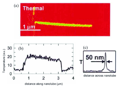
Figure 6: (Color online) Scanning thermal microscopy (SThM) of a 10nm diameter multiwall carbon nanotube. (a) Full thermal image. (b) A cut along the nanotube. (c) A cut across the nanotube. Taken from Cahill et al. (2003).

Despite the difficulty in measuring directly local temperatures of nanoscale systems, we have witnessed much progress in this direction over the last years. The first concepts of local temperature measurements are reviewed by Cahill et al. Cahill et al. (2003). Especially noteworthy are experiments where a thermocouple (serving as a thermostat) is mounted on top of an STM tip, thus creating a “scanning thermal microscope” (SThM). This device was then used to study the local temperature of a carbon nanotube placed on a substrate (see Fig. 6). The authors of this work discuss several possible shortcomings and limitations of SThM studies: the dependence of the measured temperature on topography of the sample and surface chemistry, the fact that the tip itself might perturb the sample (e.g., via near-field radiation, or by effectively cooling it), only surfaces can be measured, some of the heat is delivered through the air between the sample and tip, etc. These issues render this method hard for quantitative analysis, although some progress has been achieved Grover et al. (2006); Kim et al. (2008). We are unaware of any theoretical work (other than the one presented in this review) which has been directly related to SThM measurements.

In mesoscopic systems (e.g., quantum dots etched in 2D electron systems) which are of typical sizes of microns, tremendous advance in local thermometry has been achieved, as summarized in the thorough review by Giazotto et al. Giazotto et al. (2006). In these systems, thermometry is achieved by analyzing some temperature-dependent function (current, conductance, etc.) from which, by using known properties of the electronic surroundings, the temperature can be extracted. To give a specific recent example, by analyzing the derivatives of the current as a function of temperature and voltage, Hoffmann et al. Hoffmann et al. (2009) were able to measure the temperature gradient across a current-carrying quantum dot of $15$nm length, with the conclusion that the heat flow is mediated by phonons in the quantum dot.

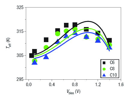
Figure 7: (Color online) Effective temperature of a molecular junction, for three different types of molecules $n$-alkanedithiol, with $n=6$ (squares), $n=8$ (circles) and $n=10$ (triangles). The solid lines are theoretical estimates from Eq. 15. From Huang et al. Huang et al. (2007).

Other options for measuring the local temperature are available. One method is to study the force at which a molecular junction breaks as a function of current. The idea behind this method is that the higher the temperature of the structure, the less external force is needed to break it Huang et al. (2007); Tsutsui et al. (2008a, b). From this force one can then extract an effective temperature. For example, Schulze et al. Schulze et al. (2008) have studied the breakdown of a molecular junction composed of a C₆₀ molecule, and showed directly that better cooling of the junction is achieved when the coupling between the molecule and the leads is improved.

Using the above method, in a recent series of experiments, Huang et al. Huang et al. (2007, 2006) have studied the local temperature of single-molecule (alkanethiols) junctions as a function of voltage bias. Their results, shown in Fig. 7 (points) indicate that with increasing voltage, the local temperature first increases, saturates, and then slightly decreases. This is in agreement with the prediction of Eq. 15 (solid lines), and suggests that electron-electron interactions indeed occur in these junctions. The same experiment also confirms that longer alkanethiol molecules heat up less due to increased electronic resistance, at fixed voltage Chen et al. (2005b).

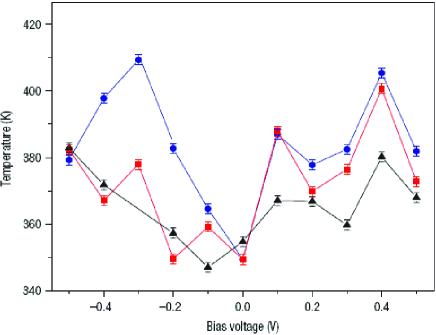
Figure 8: (Color online) Effective temperature of a molecular junction measured using Raman scattering; from Ioffe et al. Ioffe et al. (2008). The different points correspond to different modes, and while the temperature is slightly different, the overall voltage dependence shows roughly similar features. Note also the apparent decrease in the local temperature with bias, which is in line with the results of Huang et al. Huang et al. (2007).

An alternative method to study the local temperature has been suggested recently. It makes use of Raman spectroscopy and it was first applied to the study of a suspended nanotube Bushmaker et al. (2007); Deshpande et al. (2009). In these measurements, the local temperature was deduced from the shifts in the local Raman $G_{+}$ and $G_{-}$ bands of the nanotubes. The authors compared two nanotubes of lengths $2\mu$m and $5\mu$m, and found that the longer nanotube was less heated, an effect which was attributed to the thermalization of hot phonons at the center of the nanotube.

Along the same lines, the local temperature of a molecular junction has been investigated via Raman spectroscopy Ioffe et al. (2008). The idea is that the ratio between the Stokes and anti-Stokes intensities is directly related to their non-equilibrium populations in the presence of electronic current. The method has been discussed theoretically in detail Ioffe et al. (2008); Galperin et al. (2009a). In Fig. 8 the effective temperature is plotted as a function of voltage bias, for different Raman modes. From the figure one can see that although the temperature is slightly different between different modes (due to the different electron-phonon coupling strengths and symmetries), the overall voltage dependence shows roughly similar features. Note also the apparent decrease in the local temperature, which is in line with the results of Huang et al. Huang et al. (2007). This study, along with the one described before, indicate that local Raman spectroscopy may serve as a valuable tool for the study of local temperatures at the nanoscale.

III.4 Fourier’s law at the nanoscale

Let us now end this section with a somewhat different issue, that of the onset of Fourier’s law, Eq. (1), in nanostructures. As previously noted, in the context of nanoscale junctions, there is not much point in discussing the scaling of the thermal conductivity $\kappa$, which pertains to an asymptotic relation, strictly valid in the limit of large system lengths. Therefore, here we limit our discussion to the simple question of what is the temperature profile along the junction.

In the context of Fourier’s law, this question has been widely studied for both classical Lepri et al. (2003) and quantum systems Michel et al. (2006). The main focus has been on either spin-chains (i.e., Ising-like models) Michel et al. (2006); Wu and Segal (2008) or harmonic oscillator chains. The local temperatures are usually evaluated by calculating the averages of some local energy operators Saito (2003); Mejia-Monasterio and Wichterich (2007); Michel et al. (2006, 2003), or by using self-consistent thermal baths Dhar and Roy (2006); Dhar (2008); Roy (2008); Jacquet (2009). In the first case, one assumes that the local energy is related to the temperature via a local Boltzmann relation Dubi and Di Ventra (2009b), or directly proportional to the temperature via a local equipartition law Michel et al. (2003). The disadvantage of this method is two-fold: (i) there is some arbitrariness in choosing the local energy operator, since one can represent the same Hamiltonian in different ways Wu and Segal (2009), and (ii) this method assumes from the outset that the system is in a local thermodynamic equilibrium, which may not always be the case.

In the second approach, the system is attached to local heat baths. The heat current between the junction (or quantum wire) and the local baths is calculated, and the temperatures of the heat baths are determined in such a way that the heat current between the wire and the baths vanishes. This method was recently described in detail and applied to a quantum chain of non-interacting harmonic oscillators Roy (2008) and a chain of quantum dots Jacquet (2009). For instance, in Roy (2008), using quantum Langevin equations, the local temperature as a function of position was calculated for different chain lengths and for different coupling between the wire and the local baths. The conclusion of this work is that the coupling between the wire and the baths determines a length scale (mean-free path), and the heat transport crosses over from a diffusive regime (uniform temperature gradient) to a ballistic regime (uniform temperature, vanishing gradient) depending on the system length being longer or shorter than the mean free path, respectively. Since the dynamics of the system is calculated in the presence of the local baths, this shows that the properties calculated (i.e., local temperature) pertain to the combined system of quantum chain and thermal baths, and thus naturally depends on, e.g., the coupling strength between them.

Recently, a method has been suggested to calculate the local temperature of electrons in a nanoscale junction Dubi and Di Ventra (2009d); Dubi and Di Ventra (2009c). Its starting point is the stochastic Schrödinger equation (see Eq. (26)), which for non-interacting electrons reduces to a quantum master equation Pershin et al. (2008). In this approach the finite electronic system is coupled to two local heat baths at the edges of the system, in similarity to the study presented above for a chain of harmonic oscillators. In order to evaluate the local temperature, the definition we introduced in Sec. II.1 has been used. Namely, a third environment is coupled locally to the system at the position where the temperature needs to be evaluated. The properties of the system are then evaluated twice: once with the additional environment (so-called “tip”, as it mimics, e.g., the operation of a thermostat mounted on an STM tip) and once without the probe. The temperature of the probe is then varied (floated) such that a minimal change in some local (or global) properties of the system, such as its local electron density, occurs. A scan of the local temperature of the whole system can then be obtained with this method. The advantage of this approach is that it can, in principle, be implemented experimentally, and it provides the local temperature of the electrons without further scattering from other sources. In addition, it can be shown analytically that the above definition reduces to the standard thermodynamic temperature in limiting cases, for instance, in local equilibrium (see also Di Ventra and Dubi (2009)) or for two-level systems.

For the case of a wire coupled to two electrodes at different temperatures, it was found that the local temperature of the wire may exhibit quantum oscillations for intermediate lead-wire couplings Dubi and Di Ventra (2009d). Similar oscillations were later observed for a driven quantum wire Caso et al. (2010) and reflect the quantum coherent nature of the system. When the lead-wire coupling is large enough a uniform temperature ensues. In this limiting (ballistic) case, one also finds that the non-equilibrium distribution function of the system is an average of the distribution functions of the left and right baths. The fact that the temperature is uniform in the wire demonstrates the known result that for a clean system, Fourier’s law is invalid.

In order to reconstruct Fourier’s law (with an associated temperature gradient), diagonal disorder was introduced in the wire (which localizes the electronic wave-functions), and the local temperature was averaged over disorder realizations Dubi and Di Ventra (2009c). It was found that for large enough disorder, a local uniform temperature gradient ensues, giving rise to Fourier’s law. This result was interpreted in terms of an effective thermal length which controls the scale of the temperature gradient Dubi and Di Ventra (2009b). By adding the effect of dephasing the model was also able to explain the results by Roy Roy (2008) described above. We finally conclude that for the above model the onset of Fourier’s law coincides with the onset of chaos Dubi and Di Ventra (2009c). This has also been found in other model systems Michel et al. (2006); Gaul and Büttner (2007), but not in all cases Lepri et al. (1997); Li et al. (2002). Thus, this result does not appear to be universal.

IV Thermopower

IV.1 Introduction and basic definitions

In this section we discuss the concept of thermopower in nanoscale junctions. As prototypical examples that show all main features of the problem we will be focusing mainly on experiments in molecular junctions Reddy et al. (2007) and briefly mention experiments in mesoscopic systems and nanowires. The thermopower phenomenon corresponds to the case in which a temperature difference at two sides of a given junction induces a voltage drop across it. From a technological point of view, this effect is of great importance, since it may be used to recover part of the heat wasted in physical processes and generate electrical power with no moving mechanical parts. It is also of basic scientific interest, since, by combining energy and charge flow, it may encode information about the system dynamics which is unavailable in charge transport experiments Segal (2005).

The configuration we have in mind is again a junction composed of two leads separated by a nanoscale element - a quantum dot, a molecule, nanotube, etc. Consider such a junction, where the two leads are held at different temperatures, $T_{\mathrm{L}}$ and $T_{\mathrm{R}}$. The corresponding temperature difference $\Delta T=T_{\mathrm{R}}-T_{\mathrm{L}}$ gives rise to both a heat current (discussed in Sec. II) and a charge current. If the circuit is closed, after a transient time charges accumulate on one side of the junction and deplete on the other, so that a zero charge current is achieved and a voltage drop across the junction is formed. If the circuit is open (namely it is connected to an electron source), and a voltage difference $\Delta V$ is applied between the two leads with appropriate sign, a bias-induced electric current can cancel out the thermally-induced current. Note, however, that given a temperature difference the two procedures may not yield the same voltage difference. In fact, the voltage difference may also depend on the location along the system where it is probed.

The thermopower $S$ is defined as (minus) the amount of voltage $\Delta V$ at the state of vanishing current,

$$S=-\left.\frac{\Delta V}{\Delta T}\right|_{I=0}~{}~{},$$ (16)

in the limit of $\Delta T\to 0$.

This definition can also be understood from the current expressed in linear response. This is defined as

$$I=G\Delta V+L_{T}\Delta T,$$ (17)

where $G$ is the electrical conductance and $L_{T}$ is a response coefficient related to the energy flow. From this expression one readily sees that $S=L_{T}/G$. Therefore, in order to determine $S$, one has to determine the conductance $G$ and the thermal response $L_{T}$.

Before we proceed to discuss different theoretical and experimental aspects of the thermopower, it is important to ask the following question: is knowledge of the thermopower $S$ sufficient to design devices that operate as efficient heat-voltage converters? In fact, in a real device, it is not at all clear that the system is, under the given experimental conditions, in the linear response regime. Nor it is obvious that the best conversion should be achieved in that regime Esposito et al. (2009); Dubi and Di Ventra (2009d).

To this end, it is useful to define the unit-less “figure of merit”,

$$ZT=\frac{GS^{2}}{\sigma_{th}/T}~{}~{},$$ (18)

where $T$ is the temperature of the system Mahan and Sofo (1996). The quantity $ZT$ describes the efficiency of a real device or material as a thermo-electric converter. While an exact relation between $ZT$ and thermodynamic efficiency is available Müller (2008), this choice can be intuitively understood: $S$ measures how large a voltage drop can develop for a given temperature gradient, $G$ measures how easy charges can cross the junction to generate that voltage drop, and $\sigma_{th}$ measures how hard it is to maintain a temperature gradient.

It is commonly stated that for applications, one must achieve $ZT>>1$ (in fact $ZT>4$ would already be a great advance Majumdar (2004)). However, such a situation is hard to obtain: in most cases the electrical conductivity $\sigma$ and thermal conductivity $\kappa$ are related via the Wiedemann-Franz law Ashcroft and Mermin (1976), which states that

$$\frac{\kappa}{\sigma}=\left(\frac{\pi^{2}k_{B}^{2}}{3e^{2}}\right)T,$$ (19)

with the quantity in parenthesis commonly referred to as the “Lorenz number”. This means that it is difficult to increase $\sigma$ and $S$ without also increasing $\kappa$, and vice versa. However, deviations from the Wiedemann-Franz law have been observed Appleyard et al. (2000) and discussed theoretically in various systems, including Luttinger liquids Rejec et al. (2002); Kubala et al. (2008); Murphy et al. (2008); Garg et al. (2009); Kane and Fisher (1996); Li and Orignac (2002). These deviations are attributed to interactions, where the simple single-particle theory fails (see Sec. IV.3 on theoretical methods), and are exactly what is required in order to increase the efficiency of thermoelectric devices.

IV.2 Experiments on thermopower at the nanoscale

Measurements of thermopower are conceptually easier than those of thermal conductance: one applies a temperature gradient across the junction, and measures the ensuing voltage in a closed circuit when the transient current vanishes. Or, in an open circuit, one supplies a voltage to compensate for the thermally-induced current. The slope of the resulting voltage-temperature gradient curve gives the thermopower. However, in an actual experiment, particular care needs to be taken to extract this quantity. The reason is because the voltage probe that is connected to the system in order to measure the thermopower is necessarily invasive, since the applied thermal gradient would induce, locally at the voltage probe contact, an extra voltage difference. This extra effect needs to be subtracted to get the actual thermopower of the nanojunction. In addition, the ensuing voltage (including its sign) is very sensitive to the junction geometry and thus may fluctuate considerably in an actual experiment, providing non-trivial distributions of the voltage as a function of thermal gradient, from which a single voltage value may not always be easy to extract.

Before reviewing some recent experiments on nanoscale junctions, it is of interest to briefly survey some of the older experiments on mesoscopic systems as well. We point out that while most of these experimental results may be understood in terms of a linear response scattering theory (see next Sec. IV.3), some recent results, such as the appearance of additional peaks in the distribution of induced voltages versus temperature gradient (Scheibner et al., 2005), are yet to be completely accounted for. The discovery of pronounced mesoscopic effects such as Coulomb blockade and conductance quantization prompted the study of thermopower in quantum point contacts Molenkamp et al. (1990); van Houten et al. (1992b); Molenkamp et al. (1994) and quantum dots Staring et al. (1993); Godijn et al. (1999); Scheibner et al. (2005). These devices are defined by depositing gates on top of a two-dimensional electron gas formed in a semiconductor interface (typically GaAs/AlGaAs). Heating of one side of the device is achieved by passing current through it with consequent Joule heating and temperature rise. Most of the results of these experiments are well understood within the simple, single-particle picture of thermopower van Houten et al. (1992b), which will be described below.

Another, more recent batch of thermopower experiments are those conducted on nanowires, namely wires with nanoscale diameter, but extending in the longitudinal direction as long as a few microns. Various experiments were performed on wires of different materials Boukai et al. (2006, 2007); Hochbaum et al. (2007); Duarte et al. (2009); Seol et al. (2007); Lee et al. (2009), as well as carbon nanotubes Kong et al. (2005); Small et al. (2003); Sumanasekera et al. (2002). These experiments suggest that in these systems it is possible to either increase $S$ (by designing the system to have an increased electronic density of states) or reduce the thermal conductance independently by, e.g., designing a system which is smaller than the phonon mean-free-path but still larger than the corresponding mean-free-path of the electrons or holes, thus increasing the figure of merit. Specifically, in Si nanowires these are obtained by the combined effect of the change in phonon spectra and enhanced scattering off the boundary, both having little effect on the electronic part (see recent review by Rurali, Rurali (2010)). Along similar lines, boundary effects seem to highly reduce the thermal conductance but leave the charge conductance roughly unchanged Majumdar (2004).

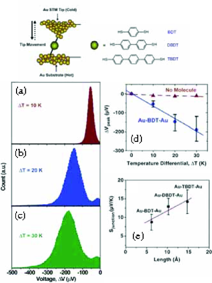
Figure 9: (Color online) Upper panel: schematic representation of thermopower experiments on molecular junctions. (a-c) Distribution of thermo-voltages obtained at different temperature gradients. Note the widening of the distributions and their non-trivial structure. (d) The most-probable thermo-voltage obtained from (a-c) as a function of the temperature gradient. The derivative of the linear fit of this curve yields the thermopower $S$. (e) $S$ of various molecules, in terms of the molecule’s length (adapted from Reddy et al.Reddy et al. (2007)).

A set of experiments which is of great interest both from an academic and technological point of view, are those performed on junctions of nanometer length, such as metallic contacts Ludoph and Ruitenbeek (1999) or molecular junctions Reddy et al. (2007); Baheti et al. (2008); Malen et al. (2009b, a); Tan et al. (2010). The latter ones are of interest since, as we will discuss in Sec. IV.3, theoretical arguments suggest that molecular junctions may exhibit large thermopower. In these latter experiments, a gold STM tip is placed on top of a gold substrate which is covered with various molecules. As the STM tip touches (and is attached to) a molecule, a thermal gradient is applied and the thermopower is measured by applying a voltage so that no current passes through the junction (see upper panel of Fig. 9). This procedure is repeated many times and a histogram of the voltage required to achieve vanishing current is obtained (for different temperature gradients, $\Delta T=10K,20K,30K$, Fig. 9(a-c)). The authors of this work then plot the voltage with maximum probability (i.e., the position of the peak in the voltage histograms) as a function of $\Delta T$, and by fitting the resulting curve with a linear fit the thermopower is obtained (Fig. 9(d)). These experiments were performed with various kinds of molecules, and interesting phenomena such as a length dependence of the thermopower (Fig. 9(e)) or strong dependence of the molecular end-groups were observed. The experiments indicate that indeed molecular junctions have favorable thermoelectric properties, suggesting that devices incorporating molecular junctions or arrays (for instance metallic plates separated by a molecular layer) may be good candidates for thermoelectric applications.

Let us, however, point out some features of the experiments which at present do not have a satisfactory theoretical explanation. For instance, as seen in Fig. 9(c), the voltage histograms have a well-defined structure, with a not so negligible secondary peak near $\Delta V=0$. Note also that the distributions cross the $\Delta V$=0 line into negative values, not shown in the figure. An additional feature of the histograms is their apparent widening with increasing temperature gradient. These fluctuations effects have been recently studied experimentally Malen et al. (2009a) and are attributed to variations in contact geometry and orbital hybridization, as well as intermolecular interactions, in accord with theoretical studies Dubi and Di Ventra (2009d).

The analysis of the above results has been done based on the single-particle (non-interacting) Landauer approach to thermopower. As it will be discussed in Sec. IV.3, in the linear response single-particle theory of thermopower, $S$ can be simply related to the electronic properties of the junction, and specifically in molecular junctions, to the position of the electrochemical potentials of the leads with respect to the gap between the highest occupied molecular orbital (HOMO) and the lowest unoccupied molecular orbital (LUMO). Since the position of the HOMO-LUMO gap affects charge transport in molecular junctions Nitzan and Ratner (2003), measurements of $S$ were suggested as a way to probe the energy position of these levels Paulsson and Datta (2003); Baheti et al. (2008). In the experiments Reddy et al. (2007); Baheti et al. (2008), a comparison of the thermopower and conductance with numerical simulations using ground-state DFT within the Landauer approach has been performed. From this comparison it was then concluded that the position of the HOMO-LUMO gap can be thus determined. This analysis, however, raises several questions. The applicability of a linear-response single-particle theory was questioned by the authors themselves Reddy et al. (2007), following the fact that the temperature differences can be tens of degrees Kelvin. In fact, one could ask if this is the smallest energy scale in the experiment. Specifically, is this energy smaller than, say, the coupling energy between the molecule and the substrate? The answer to this question is unclear, especially in light of the large error bars shown in Fig. 9(d). In addition, the non-trivial structure of the fluctuations in the voltage histogram implies that non-equilibrium effects may come into play, which are not taken into account in the linear response theory. Finally, electron-electron and electron-phonon interactions may play a crucial role in this problem.

Despite these open questions, the experiments described above are very impressive and important for the field and there are many interesting future directions to which they could be taken. For example, it would be interesting to study the change in the width of the distributions and their structures as the overall temperature is reduced. This would determine, e.g., if these distributions are due to static or dynamic effects. Another interesting direction would be to study, for several molecular structures, not just the most-probable voltage, but the real (statistical) average of the distributions, and infer from this whether the resulting thermopower displays the same features as reported above (e.g., length dependence, etc.), and whether this quantity matches calculations based on single-particle theories.

IV.3 Theoretical methods

In this subsection we describe the present theoretical methods available to describe the phenomenon of thermopower. The most common one is based on the Landauer approach with its most common implementation within ground-state DFT. As we will discuss, this approach has several advantages, being rather computationally straightforward, and having a rather simple physical interpretation. However, we will argue that in many cases of actual experimental interest, it may be inadequate, since it is based on the usual assumptions of scattering theory of non-interacting electrons. In addition, as we have emphasized also in Sec. II.3.1, the use of ground-state DFT is questionable in an intrinsically non-equilibrium problem as that discussed here. We will then introduce an approach based on the theory of open quantum systems, which is ideally suited for the present problem and can, in principle, account for interactions (beyond mean-field). The latter point has its most practical implementation in an extension of time-dependent DFT to open quantum systems Di Ventra and D’Agosta (2007); D’Agosta and Di Ventra (2008b).

IV.3.1 Single-particle theory of thermopower

The starting point for calculating the thermopower within a single-particle picture is the Landauer expression for the electrical current Butcher (1990),

$$I=\frac{e}{\pi\hbar}\int^{\infty}_{-\infty}\mathrm{d}\epsilon{\mathcal{T}}(\epsilon)\left[f_{\mathrm{L}}(\epsilon)-f_{\mathrm{R}}(\epsilon)\right]~{}~{},$$ (20)

where ${\mathcal{T}}(\epsilon)$ is the transmission coefficient at energy $\epsilon$ and $f_{\mathrm{L},\mathrm{R}}$ are the Fermi distributions of the left and right leads. In the limit of small bias and temperature gradient (i.e., $|\Delta T|<<T$ and $|e\Delta V|<<\mu$, where $T$ is the background temperature and $\mu$ is the equilibrium chemical potential) the distribution functions are approximately given by Butcher (1990) ($i=L,R$)

$$f(\epsilon,\mu_{i},T_{i})\simeq f(\epsilon,\mu,T)\pm\frac{\mathrm{d}f}{\mathrm{d}\epsilon}(\mu-\mu_{i})\mp\frac{\mathrm{d}f}{\mathrm{d}\epsilon}(\epsilon-\mu)\frac{(T_{i}-T)}{T}~{},$$ (21)

where now $f(\epsilon)$ is the equilibrium distribution, and the $+$ and $-$ sign correspond to which electrochemical potential is higher or lower in energy with respect to the equilibrium chemical potential. Inserting this into Eq. (20) and equating the current to zero, one obtains

$$S(T)=\frac{1}{eT}\frac{\int^{\infty}_{-\infty}\mathrm{d}\epsilon{\mathcal{T}}(\epsilon)(\epsilon-\mu)(-f^{\prime}(\epsilon))}{\int^{\infty}_{-\infty}\mathrm{d}\epsilon{\mathcal{T}}(\epsilon)(-f^{\prime}(\epsilon))}~{}~{}.$$ (22)

Already from this result several features may be seen. First, since at $T=0$ we have $-f^{\prime}(\epsilon)=\delta(\epsilon-\mu)$, the numerator of $S$ vanishes and $S(T=0)=0$. Second, even at finite temperatures $f^{\prime}(\epsilon)$ is symmetric around $\mu$, and therefore $S=0$ unless ${\mathcal{T}}(\epsilon)$ is not symmetric around $\mu$. This is similar to the condition in bulk materials that requires the particle-hole symmetry be broken to have a finite thermopower Ashcroft and Mermin (1976).

One can further simplify $S(T)$ by taking the low-temperature limit and by assuming that there are no electronic resonances close to the equilibrium chemical potential. Using the Sommerfeld expansion to first order around $\mu(T=0)=\epsilon_{F}$ Ashcroft and Mermin (1976) one has

$$\int^{\infty}_{-\infty}{\mathcal{T}}(\epsilon)(\epsilon-\mu)f^{\prime}(\epsilon) \approx \left.\frac{\pi^{2}}{6}k_{B}^{2}T^{2}\frac{\mathrm{d}^{2}[{\mathcal{T}}(\epsilon)(\epsilon-\mu)]}{\mathrm{d}\epsilon^{2}}\right|_{\epsilon_{F}}$$ (23)

$$= \frac{\pi^{2}}{3}k_{B}^{2}T^{2}{\mathcal{T}}^{\prime}(\epsilon)$$

(where the second derivative comes from integration by parts) and one arrives at the expression for the thermopower,

$$S=\frac{\pi^{2}}{3}\frac{k_{B}}{e}k_{B}T\left.\frac{\mathrm{d}\ln({\mathcal{T}}(\epsilon))}{\mathrm{d}\epsilon}\right|_{\epsilon_{F}}~{}~{},$$ (24)

which is similar to Mott’s semiclassical formula for bulk metals Ashcroft and Mermin (1976); Lunde and Flensberg (2005). We stress once more that this approximation is only valid at low temperatures and away from transmission resonances, so that the variation in ${\mathcal{T}}(\epsilon)$ is small.

The advantages of using the Landauer formalism are evident: it provides both a simple interpretation of the thermopower in terms of single-particle properties such as the transmission coefficient ${\mathcal{T}}(\epsilon)$, and a rather straightforward computational procedure. In fact, one only needs to determine the transmission coefficient ${\mathcal{T}}(\epsilon)$, which can be done as discussed in Sec. II.3.1. These reasons have made this approach extremely popular and widely used. An early use of Eq. (24) is in the study of thermopower in quantum point contacts Molenkamp et al. (1990); van Houten et al. (1992b); Molenkamp et al. (1994) and quantum dots Staring et al. (1993). In these mesoscopic systems, a gate voltage is used to tune either the width of the quantum point contacts or the energy levels in the quantum dots, giving rise to quantized conductance and Coulomb blockade. It turns out that in the cases above, the Landauer approach yields reasonably good agreement between theory and experiment Molenkamp et al. (1990), and knowledge of ${\mathcal{T}}(\epsilon)$ reasonably describes both the conductance and the thermopower. This would naively suggest that for these types of systems, the above single-particle picture accounts for most of the thermopower. However, more recent investigations which include effects of interactions, show that in both types of systems interactions may induce deviations from the Wiedmann-Franz law, thus reducing the agreement with experiments Kubala et al. (2008); Lunde et al. (2006); Turek et al. (2005); Turek and Matveev (2002); Zhang (2007), suggesting that the agreement in the single-particle case may be the result of cancelation of errors.

In fact, despite its simplicity, the above approach suffers several shortcomings of particular relevance in nanoscale systems. The most prominent is the fact that it is formulated for non-interacting electrons. This means that any inclusion of interaction effects directly into ${\mathcal{T}}(\epsilon)$ can only be done at the mean-field level Vignale and Di Ventra (2009). To correct this, one should abandon the Landauer formula for the current, and, alternatively, use expressions for the currents obtained by using, e.g., the NEGF Meir and Wingreen (1992) or rate equations Koch et al. (2004). To our knowledge, in its fully interacting form NEGF was never employed to study the effects of electron interactions on the thermopower of molecular junctions.

Another limitation of the Landauer approach is the erroneous result it supplies in the zero-coupling limit. To demonstrate this, consider the simplest model for a nanoscale junction: a single resonant level symmetrically coupled to leads with spinless electrons (adding spin simply introduces a factor of two). The transmission is given by a Breit-Wigner formula, ${\mathcal{T}}(\epsilon)=\Gamma^{2}/(\Gamma^{2}+(\epsilon-\epsilon_{F})^{2})$, where $\Gamma$ is the lead-induced level broadening. Substituting into the expression for $S$ (Eq. (24)) and taking the limit of $\Gamma\to 0$ gives a finite value, $S=-\frac{2\pi^{2}}{3}\frac{k_{B}^{2}}{e}\frac{T}{\epsilon-\epsilon_{F}}$. However, if one would consider a real device, it is clear that by detaching the leads would result in no temperature-induced voltage drop. The reason for this discrepancy is simple: in the linear response calculation one assumes that the temperature difference is the smallest energy scale, yet in the limit $\Gamma\to 0$, $\Gamma$ becomes comparable to such a scale, and the approximation breaks down. One should thus be careful both in using perturbation theory in the coupling between the leads and, say, a molecule in the junction and in comparing such calculations to experiments (see Sec. IV.3.2).

Much of the recent theoretical work on thermopower has been devoted to molecular junctions. Before we review some recent results, it is important to understand the origin of the specific interest in such systems, which may be understood from analyzing the Landauer formula (24). In a molecular junction, the Fermi energy of the leads is placed somewhere between the HOMO and the LUMO (i.e., in the HOMO-LUMO gap) Nitzan and Ratner (2003). The question is where exactly? The answer to this question cannot be answered by studying the conductance (or transmission) alone, which can be demonstrated through a simple example Paulsson and Datta (2003). Consider such a molecular junction, with HOMO and LUMO energies $\epsilon_{\text{HOMO}}$ and $\epsilon_{\text{LUMO}}$, respectively. The transmission function can be modeled by a double Lorenzian, corresponding to tunneling via each of these levels independently, and assumes the following form,

$${\mathcal{T}}(\epsilon)=\frac{\Gamma_{\mathrm{L}}\Gamma_{\mathrm{R}}}{\tilde{\Gamma}^{2}+\left(\epsilon_{F}-\epsilon_{\text{HOMO}}\right){}^{2}}+\frac{\Gamma_{\mathrm{L}}\Gamma_{\mathrm{R}}}{\tilde{\Gamma}^{2}+\left(\epsilon_{F}-\epsilon_{\text{LUMO}}\right){}^{2}}~{}~{},$$ (25)

where $\Gamma_{\mathrm{L},\mathrm{R}}$ is the level broadening due to the left (right) lead and $\tilde{\Gamma}=(\Gamma_{\mathrm{L}}+\Gamma_{\mathrm{R}})/2$. (For simplicity, we assume it to be the same for the two levels.) The resulting thermopower (in units of $\frac{\pi^{2}}{3}\frac{k_{B}^{2}}{e}T$), along with the transmission coefficient, is plotted in Fig. 10 (taking $\tilde{\Gamma}/(\epsilon_{\text{LUMO}}-\epsilon_{\text{HOMO}})=0.1$). As seen, according to this simple model, for a given value of transmission between $\epsilon_{\text{LUMO}}$ and $\epsilon_{\text{HOMO}}$, there are two values of the Fermi energy which provide a solution to Eq. (25), and hence conductance alone does not suffice to determine the position of the Fermi energy. From the same model, however, one would infer that the sign of the thermopower is determined by the position of the Fermi energy from the center of the HOMO-LUMO gap, similarly to the fact that the sign of the thermopower in bulk materials is determined by whether the conductance is dominated by electrons or holes Ashcroft and Mermin (1976), and therefore the sign of thermopower distinguishes between the two Fermi energies which solve Eq. (25).

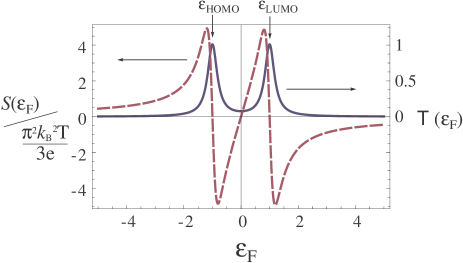
Figure 10: (Color online) Transmission (solid line) and normalized thermopower (dashed line) as a function of the position of the Fermi energy with respect to the HOMO-LUMO gap, based on the Landauer formula, Eq. (24), with approximation Eq. (25).

This idea, along with the prospect of using molecular junctions as efficient thermoelectric devices, has generated much theoretical interest. To give a few examples, Segal Segal (2005) showed that by measuring the thermopower one can distinguish between different electron transport mechanisms. Thermal and vibrational effects were studied in detail Koch et al. (2004) using rate equations, and it was shown that at low temperatures the signature of the vibrational modes on the thermopower can be measured. Murphy et al. Murphy and Moore (2007) used rate equations to study the optimization of the figure of merit of a molecular junction, in similarity to the optimization of the figure of merit in bulk thermoelectrics Mahan and Sofo (1996).

Much recent attention has been devoted to studying thermopower of molecular junctions using ground-state DFT to calculate ${\mathcal{T}}(\epsilon)$ combined with the Landauer formula (22) (or its even more simplified version Eq. (24)) Finch et al. (2009); Paulsson and Datta (2003); Zheng et al. (2004); Pauly et al. (2008); Ke et al. (2009); Müller (2008); Wang et al. (2005); Liu and Chen (2009); Liu et al. (2009b). In some cases, it has also been reported an impressive agreement between the theoretical results and experiments Ke et al. (2009).

However, caution has to be applied in making such claims. In fact, if the system is away from linear response - and many experiments so far likely correspond to such case - given a temperature difference, setting $I=0$ in Eq. 20 does not necessarily provide a unique solution for the potential difference. In other words, there may be more than one potential difference $\Delta V$ that gives rise to the same $\Delta T$ (and hence several values of thermopower for the same temperature difference), when $I=0$, as it is permitted by the non-linearity of Eq. 20. In addition, as already emphasized previously, even if the single-particle equations (22) and (24) were good starting points to describe the problem at hand, ground-state DFT is fundamentally flawed in the present context (even if one knew the exact ground-state functional) due to the fundamental non-equilibrium nature of the problem Vignale and Di Ventra (2009); Bushong et al. (2005); Di Ventra and Todorov (2004); Di Ventra (2008). In this respect, even the interpretation of ground-state Kohn-Sham orbitals is questionable, since the latter ones are auxiliary quantities whose only role is to provide the correct density of the corresponding many-body system in its ground-state.

To these limitations we must also add few more physical issues. When a thermal gradient is applied to a junction, the transient dynamics is fundamental in establishing the voltage difference that enters the definition of thermopower. Since the dynamical formation of local resistivity dipoles creates strong local fields at the junction (especially at the nanoscale), these fields influence the electron motion in a non-trivial way, and thus influence the long-time behavior of the carrier dynamics, even in the dc limit. This is particularly important away from linear response Di Ventra (2008), which may be the experimental case.

It is the self-consistent formation of these fields that makes the thermopower very sensitive (both in magnitude and sign) to atomic details, and thus to the contact geometry between the nanostructure and bulk electrodes, as demonstrated also experimentally Ludoph and Ruitenbeek (1999). This precludes an easy interpretation in terms of “electron” or “hole” excitations as in bulk metals, and thus an easy relation with single-particle states (such as the HOMO and LUMO) as the Landauer equation (22) would imply. All this points to the fact that, since the system is in dynamical interaction with two different baths, one needs to go beyond the approximations underlying Eq. (22), and consider an open quantum system approach.

IV.3.2 An open quantum system approach

The present authors have precisely explored the problem of thermopower within the theory of open quantum systems Dubi and Di Ventra (2009d). In analogy with the idea that electrical currents may be studied using finite systems Di Ventra and Todorov (2004); Bushong et al. (2005), one can study a finite system in contact with two heat baths held at different temperatures (i.e., finite leads connected by a nanoscale constriction, either a molecule, wire, etc.). If the system has a finite thermoelectric response then charges would flow between the leads until the ensuing electric potential “balances” the thermal gradient, and a charge imbalance is created between the two leads (which is related to the thermo-voltage via the Poisson equation). Note that in this approach the system is allowed to find its own charge distribution via the transient dynamics (unlike a static approach where a static distribution is imposed a priori via boundary conditions), and even when the charge current is zero an energy current is still present, as in the actual experiments. Then, by calculating the thermally-induced charge imbalance one obtains information on the thermoelectric response of the junction via the usual definitions. This approach is also not limited to linear response thus providing information on the thermo-voltage even when the temperature gradient is not the smallest energy scale.

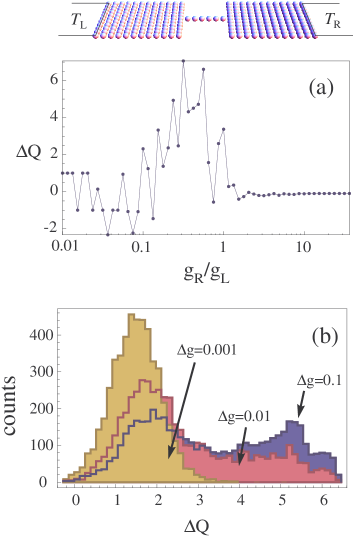
Figure 11: (Color online) Upper panel: schematic representation of the model molecular junction composed of two quasi-two-dimensional leads connected with a molecular wire. The leads are coupled to external heat baths, each at its own temperature. (a) Electron charge imbalance as a function of the ratio between the couplings $g_{R(L)}$ between the wire and the right (left) lead. A strong dependence can be observed and even a change of sign (from Dubi and Di Ventra (2009d)). (b) Distribution of charge imbalance, when the couplings between the wire and the leads are drawn from a Gaussian distribution, with an average $g=0.1$ and width $\Delta g=0.001,0.01$ and $0.1$ in units of the hopping parameter (see text).

An implementation of such an open system approach can also be formulated within time-dependent DFT, thus allowing to include, in principle, all possible dynamical many-body effects in the thermopower (recall in fact that given the baths that set the temperature differences, the ensuing electrostatic voltage is a well-defined functional of the density). Indeed, Di Ventra and D’Agosta have recently proved that if the bath-electron interactions are treated within a memory-less approximation (the thermal baths being Ohmic) Van Kampen (2001), then there is a one-to-one correspondence between the exact ensemble-averaged current density and the external vector potential, therefore extending the theorem (and Kohn-Sham scheme) of time-dependent current-DFT (TDCDFT) to open quantum systems Di Ventra and D’Agosta (2007); D’Agosta and Di Ventra (2008b). The framework for this theory (named Stochastic TDCDFT) is the stochastic Schrödinger equation, which describes a Hamiltonian quantum system in the presence of a bath (the extension to several baths is trivial) Breuer and Petruccione (2002) ($\hbar=1$),

$$\dot{\Psi}(t)=-i{\mathcal{H}}\Psi(t)-{\scriptstyle 1\over 2}\hat{V}^{\dagger}\hat{V}\Psi(t)+l(t)\hat{V}\Psi(t)~{}~{}.$$ (26)

Here $\Psi(t)$ is the many-body state vector, ${\mathcal{H}}$ is the Hamiltonian of the system (describing both the molecule, the leads and the coupling between them), $\hat{V}$ are the so-called bath operators (which could in principle be position and/or time-dependent) Van Kampen (2001), which describe transitions between the different many-body states induced by the bath(s), and $l(t)$ is a stochastic field which is taken to have zero mean and a $\delta$-function autocorrelation, $\langle l(t)\rangle=0,~{}~{}\langle l(t)l(t^{\prime})\rangle=\delta(t-t^{\prime})$.

As a first demonstration, the method was recently used by the present authors to study the thermopower of a simple model system of spinless non-interacting electrons, for which the calculations can be equivalently carried out with the density-matrix rather than the state vector, by averaging over the stochastic realizations Pershin et al. (2008). In that model two planar leads, each in contact with a thermal bath at a given temperature, are connected via a nanoscale wire (see upper panel of Fig. 11). The bath-electron interactions are described by the operators

$$\hat{V}^{L,R}_{kk^{\prime}}=\sqrt{\gamma^{L,R}_{kk^{\prime}}f^{L,R}(\epsilon_{k})}|k\rangle\langle k^{\prime}|~{}~{},$$ (27)

where $|k\rangle$ are the single-particle states of the Hamiltonian, $f^{L,R}$ is the Fermi function containing information on the left (right) bath temperature, and $\gamma^{L,R}_{kk^{\prime}}$, which are the (inelastic) transition rates between states $k$ and $k^{\prime}$, depend on the bath location (i.e., left or right) Dubi and Di Ventra (2009d). The corresponding equations of motion are then solved to obtain the wave-function, and hence the electron density, potential, and also the heat currents (see also Sec. III) at steady state.

Several interesting features are revealed by this model. For instance, the obtained thermo-voltage shows non-linear characteristics, which imply that the linear regime may not be the best regime to operate a thermo-electric device Dubi and Di Ventra (2009d). Another interesting feature is the strong dependence of the charge imbalance in the leads (and hence the thermopower) on the coupling between the wire (or molecule) and the leads. This confirms the experimental findings in metallic quantum point contacts Ludoph and Ruitenbeek (1999). In Fig. 11(a) Dubi and Di Ventra (2009d) the charge imbalance between the leads is plotted as a function of the ratio between the coupling between the wire and the left and right leads. From the figure it is obvious that the charge imbalance strongly fluctuates, and can even change sign as a function of the wire-lead coupling. To demonstrate the importance of these fluctuations and to tie with the experimental results presented in Sec. IV.2, we have performed a calculation for the same system as discussed in Dubi and Di Ventra (2009d), where the coupling constants were drawn from a normal distribution around typical values of $g=0.1t$, where $g$ is the lead-wire coupling and $t$ is the tight-binding hopping parameter, which describes the bandwidth of the leads. Other numerical parameters are the filling fraction of electrons, $n=1/3$, and the temperatures of the left and right heat baths, $T_{L}=0.1$ and $T_{R}=1$ (in units of $t$). A histogram of the resulting charge imbalance is plotted in Fig. 11(b), for three values of the width of the normal distribution, $\Delta g=0.001,0.01$ and $0.1$ (in units of the hopping parameter). While more work needs to be done to explain the experimental data presented in Fig. 9(c), these theoretical results clearly bear some resemblance to experiments by showing a double structure in the charge imbalance as a function of the coupling asymmetry.

Using Stochastic TDCDFT one can extend the above system model to interacting systems, as well as to a multi-component formulation Appel and Di Ventra (2009), whereby the Hamiltonian now contains the correlated motion of electrons and (possibly quantum) ions, with both components interacting with an external environment. Such studies would shed new light on the role of interactions and ion dynamics on thermopower, and enable a study of local heating effects in nanoscale systems (see also Sec. III). No results are, however, yet available for these cases.

V Summary and future prospects

In this review we have discussed energy transport in nanoscale systems, such as molecular junctions, suspended nanotubes, quantum point contacts, etc. Our aim was to put under a unified theme the three major issues of thermal transport, namely thermal conductance, local temperature and heating, and thermo-electricity. We have critically examined both theoretical and experimental aspects of these topics. We have presented many theoretical methods based on the single-particle scattering approach, non-equilibrium Green’s functions formalism, molecular dynamics, etc. From the experimental side we have reviewed state-of-the-art experiments, and stressed the difficulty and open questions in analyzing such experiments.

V.1 Future Prospects

We wish to conclude this review by presenting three novel ideas related to energy transport in nanoscale systems. These ideas, which deviate somewhat from the usual path of thermoelectricity and heat transport, reflect to our opinion the richness and usefulness of studying energy flow in nanoscale systems, and we hope they will stimulate both the experimental and theoretical communities.

Thermo-spintronics –   Thermo-spintronics (sometimes also called spin calorimetrics) refers to the manipulation of electron spins with thermal effects. Generating spin currents, that is the flow of electron spins, plays an eminent role in the field of spintronics, which is the spin analogue of electronics (see, e.g., Ẑutić et al. (2004)). However, manipulating spins in order to generate spin currents is quite difficult, and it is equally hard to generate a spin current without generating an accompanying charge current. In recent experiments Uchida et al. (2008, 2009) a spin-analog to the Seebeck effect was used to generate a spin-voltage, induced by a temperature difference along a ferromagnetic slab. Although this effect is rather small (compared to its charge counterpart, but larger than expected in view of spin-flip scattering) and inherently induces an electric voltage as well, it has been suggested that these shortcomings may be overcome by applying a temperature gradient to a molecular junction placed between ferromagnetic leads Dubi and Di Ventra (2009e), a setup which was further studied recently Lü et al. (2010); Wang et al. (2010); Ying and Jin (2010). In another interesting work, a variety of thermoelectric effects in magnetic junctions have been studied Hatami et al. (2007, 2009); Heikkilä et al. (2010), with unusual features such as thermal spin-transfer torque, spin-polarized cooling and spin-heat coupling effects.

Enhanced thermopower in DNA –   DNA, the basic building block of our genetic code, shows also large potential in nanotechnology applications Dekker and Ratner (2001); Di Ventra et al. (2004); Zwolak and Di Ventra (2008). In a recent study it was shown Maciá (2007, 2005), using a model Hamiltonian for different DNA-like chains, that under certain conditions, the Seebeck coefficient and figure of merit of a lead-DNA-lead junction can be quite high, and can rise to hundreds of $\mu V/$K, to be compared with a few $\mu V/$K of other single-molecule junctions studied so far. These high values of the thermopower seem to stem from transport resonance effects, which can be tuned rather easily in DNA. This, with the fact that there is a lot of know-how regarding DNA manipulation and preparation, makes DNA-based systems interesting candidates for future thermoelectric and cooling devices at the nanoscale.

Thermoelectricity in superconducting wires –   Raising the critical temperature, $T_{c}$, of superconducting materials is clearly a technologically important goal. However, most superconducting materials have a $T_{c}$ well below room temperature, even in the well-known high-$T_{c}$ materials (with $T_{c}\sim 80$K for wires and $T_{c}\sim 200$K for bulk). Recently, the present authors have suggested Dubi and Di Ventra (2009a) to study a superconducting wire held at two different temperatures at its edges. Using the method introduced in Sec. IV.3.2 combined with a self-consistent mean-field theory, it was shown that for an (ideally) clean superconducting wire, if one of the sides (the cold side) is held at low enough temperatures, the temperature of the hot side can be much larger than the equilibrium $T_{c}$, with the wire still in its superconducting state. Although this study neglects some effects (such as phase fluctuations), the basic idea is simple: in order to have a superconducting wire, instead of cooling down the entire apparatus, one can locally cool the wire by attaching to it a local refrigerator, for example one made from a Peltier cooling device Shakouri (2006). This may pave the road for hybrid superconducting circuits which operate at relatively high temperatures.

V.2 Final thoughts

These last few examples - and what we have discussed in this Colloquium - clearly show that the quest to understand energy transport in nanostructures is far from over. In fact, it seems to us that we have barely scratched the surface of this problem and more discoveries await us. Regarding thermal conductance, finding systems that show either very good (for nano-electronic applications) or very poor (for thermo-electric applications) thermal conductance is needed. As for thermoelectricity, there is a need to advance our theoretical tools quite substantially. For instance, theories that account for the statistical nature of the experiments should be developed that include also electron-electron and electron-phonon interactions on equal footing. In addition, since the problem is intrinsically out of equilibrium (even at steady-state) these theories need to include dynamical effects. As for local heating and local temperatures, the handful of experiments that have appeared recently are certainly a great start, but more are needed in order to truly determine the processes leading to heating (and cooling) in nanoscale junctions. Similarly, more experiments that could determine directly the validity (or invalidity) of Fourier’s law are highly desirable.

Due to the rapid developments in science and technology it is difficult to predict where the field will go from here. However, there is no doubt that novel and ingenious ideas will be put forward that will help us profit from energy flow, storage and conversion. Embarking in such a quest could not be more timely.

References

- Akkermans and Montambaux (2007) Akkermans, E., and G. Montambaux, 2007, Mesoscopic Physics of Electrons and Photons (Cambridge University Press).
- Ando (1991) Ando, T., 1991, Phys. Rev. B 44(15), 8017.
- Angelescu et al. (1998) Angelescu, D. E., M. C. Cross, and M. L. Roukes, 1998, Superlattices and Microstructures 23(3-4), 673 .
- Appel and Di Ventra (2009) Appel, H., and M. Di Ventra, 2009, Phys. Rev. B 80(21), 212303.
- Appleyard et al. (2000) Appleyard, N. J., J. T. Nicholls, M. Pepper, W. R. Tribe, M. Y. Simmons, and D. A. Ritchie, 2000, Phys. Rev. B 62(24), R16275.
- Ashcroft and Mermin (1976) Ashcroft, N. W., and N. D. Mermin, 1976, Solid State Physics (Brooks Cole).
- Baheti et al. (2008) Baheti, K., J. A. Malen, P. Doak, P. Reddy, S.-Y. Jang, T. D. Tilley, A. Majumdar, and R. A. Segalman, 2008, Nano Lett. 8(2), 715.
- Balandin et al. (2008) Balandin, A. A., S. Ghosh, W. Bao, I. Calizo, D. Teweldebrhan, F. Miao, and C. N. Lau, 2008, Nano Letters 8(3), 902.
- Bell (2008) Bell, L. E., 2008, Science 321(5895), 1457.
- Berber et al. (2000) Berber, S., Y.-K. Kwon, and D. Tománek, 2000, Phys. Rev. Lett. 84(20), 4613.
- Blencowe (1999) Blencowe, M., 1999, Phys. Rev. B 59(7), 4992.
- Blencowe (2004) Blencowe, M., 2004, Physics Reports 395(3), 159 .
- Bonetto et al. (2004) Bonetto, F., J. Lebowitz, and J. Lukkarinen, 2004, Journal of Statistical Physics 116(1-4), 783.
- Bonetto et al. (2000) Bonetto, F., J. L. Lebowitz, and L. Rey-Bellet, 2000, in Mathematical Physics 2000, edited by A. Fokas, A. Grigoryan, T. Kibble, and B. Zegarlinski (Imperial College Press), p. 128.
- Boukai et al. (2006) Boukai, A., K. Xu, and J. Heath, 2006, Advanced Materials 18(7), 864.
- Boukai et al. (2007) Boukai, A. I., Y. Bunimovich, J. Tahir-Kheli, J.-K. Yu, W. A. G. III, and J. R. Heath, 2007, Nature 451, 168.
- Bourgeois et al. (2007) Bourgeois, O., T. Fournier, and J. Chaussy, 2007, Journal of Applied Physics 101(1), 016104.
- Breuer and Petruccione (2002) Breuer, H. P., and F. Petruccione, 2002, Theory of Open Quantum Systems (Oxford University Press).
- Brown et al. (2005) Brown, E., L. Hao, J. C. Gallop, and J. C. Macfarlane, 2005, Appl. Phys. Lett. 87(2), 023107.
- Bushmaker et al. (2007) Bushmaker, A. W., V. V. Deshpande, M. W. Bockrath, and S. B. Cronin, 2007, Nano Lett. 7(12), 3618.
- Bushong et al. (2005) Bushong, N., N. Sai, and M. Di Ventra, 2005, Nano Lett. 5(12), 2569.
- Butcher (1990) Butcher, P., 1990, Journal of Physics: Condensed Matter 2(45), 4869.
- Büttiker et al. (1985) Büttiker, M., Y. Imry, R. Landauer, and S. Pinhas, 1985, Phys. Rev. B 31(10), 6207.
- Cahill (1990) Cahill, D. G., 1990, Review of Scientific Instruments 61(2), 802.
- Cahill et al. (2003) Cahill, D. G., W. K. Ford, K. E. Goodson, G. D. Mahan, A. Majumdar, H. J. Maris, R. Merlin, and S. R. Phillpot, 2003, Journal of Applied Physics 93(2), 793.
- Calizo et al. (2007) Calizo, I., A. A. Balandin, W. Bao, F. Miao, and C. N. Lau, 2007, Nano Letters 7(9), 2645.
- Carruthers (1961) Carruthers, P., 1961, Rev. Mod. Phys. 33(1), 92.
- Caso et al. (2010) Caso, A., L. Arrachea, and G. S. Lozano, 2010, Phys. Rev. B 81(4), 041301.
- Chalopin et al. (2008) Chalopin, Y., J.-N. Gillet, and S. Volz, 2008, Phys. Rev. B 77(23), 233309.
- Chang et al. (2006) Chang, C. W., A. M. Fennimore, A. Afanasiev, D. Okawa, T. Ikuno, H. Garcia, D. Li, A. Majumdar, and A. Zettl, 2006, Phys. Rev. Lett. 97(8), 085901.
- Chang et al. (2008) Chang, C. W., D. Okawa, H. Garcia, A. Majumdar, and A. Zettl, 2008, Phys. Rev. Lett. 101(7), 075903.
- Chen (2005) Chen, G., 2005, Nanoscale Energy Transport and Conversion (Oxford University Press, USA).
- Chen et al. (2005a) Chen, K.-Q., W.-X. Li, W. Duan, Z. Shuai, and B.-L. Gu, 2005a, Phys. Rev. B 72(4), 045422.
- Chen et al. (2008) Chen, R., A. I. Hochbaum, P. Murphy, J. Moore, P. Yang, and A. Majumdar, 2008, Phys. Rev. Lett. 101(10), 105501.
- Chen (2008) Chen, Y.-C., 2008, Phys. Rev. B 78(23), 233310.
- Chen et al. (2003) Chen, Y.-C., M. Zwolak, and M. Di Ventra, 2003, Nano Lett. 3(12), 1691.
- Chen et al. (2005b) Chen, Y.-C., M. Zwolak, and M. Di Ventra, 2005b, Nano Lett. 5(4), 621.
- Cheng et al. (2006) Cheng, C.-L., J. S. Evans, and T. Van Voorhis, 2006, Phys. Rev. B 74(15), 155112.
- Chiatti et al. (2006) Chiatti, O., J. T. Nicholls, Y. Y. Proskuryakov, N. Lumpkin, I. Farrer, and D. A. Ritchie, 2006, Phys. Rev. Lett. 97(5), 056601.
- Chiu et al. (2005) Chiu, H.-Y., V. V. Deshpande, H. W. C. Postma, C. N. Lau, C. Mikó, L. Forró, and M. Bockrath, 2005, Phys. Rev. Lett. 95(22), 226101.
- Choi et al. (2005) Choi, T. Y., D. Poulikakos, J. Tharian, and U. Sennhauser, 2005, Appl. Phys. Lett. 87(1), 013108.
- Choi et al. (2006) Choi, T.-Y., D. Poulikakos, J. Tharian, and U. Sennhauser, 2006, Nano Lett. 6(8), 1589.
- D’Agosta and Di Ventra (2006) D’Agosta, R., and M. Di Ventra, 2006, Journal of Physics: Condensed Matter 18(49), 11059.
- D’Agosta and Di Ventra (2008a) D’Agosta, R., and M. Di Ventra, 2008a, Journal of Physics: Condensed Matter 20(49), 374102.
- D’Agosta and Di Ventra (2008b) D’Agosta, R., and M. Di Ventra, 2008b, Phys. Rev. B 78(16), 165105.
- D’Agosta et al. (2006) D’Agosta, R., N. Sai, and M. Di Ventra, 2006, Nano Lett. 6(12), 2935.
- Datta (1997) Datta, S., 1997, Electronic transport in mesoscopic systems (Cambridge University Press).
- Dekker and Ratner (2001) Dekker, C., and M. A. Ratner, 2001, Physics World 14, 29.
- Deshpande et al. (2009) Deshpande, V. V., S. Hsieh, A. W. Bushmaker, M. Bockrath, and S. B. Cronin, 2009, Phys. Rev. Lett. 102(10), 105501.
- Dhar (2008) Dhar, A., 2008, Advances in Physics 57(5), 457.
- Dhar and Lebowitz (2008) Dhar, A., and J. L. Lebowitz, 2008, Phys. Rev. Lett. 100(13), 134301.
- Dhar and Roy (2006) Dhar, A., and D. Roy, 2006, Journal of Statistical Physics 125(4), 805.
- Di Ventra (2008) Di Ventra, M., 2008, Electrical Transport in Nanoscale Systems (Cambridge University Press).
- Di Ventra and D’Agosta (2007) Di Ventra, M., and R. D’Agosta, 2007, Phys. Rev. Lett. 98(22), 226403.
- Di Ventra and Dubi (2009) Di Ventra, M., and Y. Dubi, 2009, Europhys. Lett. 85(4), 40004.
- Di Ventra et al. (2004) Di Ventra, M., S. Evoy, and J. E. James R. Heflin, 2004, Introduction to Nanoscale Science and Technology (Kluwer Academic Publishers).
- Di Ventra and Lang (2002) Di Ventra, M., and N. Lang, 2002, Phys. Rev. B 65(4), 045402.
- Di Ventra and Todorov (2004) Di Ventra, M., and T. N. Todorov, 2004, Journal of Physics: Condensed Matter 16(45), 8025.
- Duarte et al. (2009) Duarte, N. B., G. D. Mahan, and S. Tadigadapa, 2009, Nano Lett. 9(2), 617.
- Dubi and Di Ventra (2009a) Dubi, Y., and M. Di Ventra, 2009a, unpublished .
- Dubi and Di Ventra (2009b) Dubi, Y., and M. Di Ventra, 2009b, Phys. Rev. E 79(4), 042101.
- Dubi and Di Ventra (2009c) Dubi, Y., and M. Di Ventra, 2009c, Phys. Rev. B 79(11), 115415.
- Dubi and Di Ventra (2009d) Dubi, Y., and M. Di Ventra, 2009d, Nano Lett. 9(1), 97.
- Dubi and Di Ventra (2009e) Dubi, Y., and M. Di Ventra, 2009e, Phys. Rev. B 79(8), 081302.
- Esposito et al. (2009) Esposito, M., K. Lindenberg, and C. V. den Broeck, 2009, Europhys. Lett. 85(6), 60010.
- Feldman et al. (2000) Feldman, J. L., D. J. Singh, I. I. Mazin, D. Mandrus, and B. C. Sales, 2000, Phys. Rev. B 61(14), R9209.
- Fermi et al. (1955) Fermi, E., J. Pasta, and S. Ulam, 1955, Los Alamos report LA-1940 .
- Finch et al. (2009) Finch, C. M., V. M. García-Suárez, and C. J. Lambert, 2009, Phys. Rev. B 79(3), 033405.
- Fourier (1822) Fourier, J., 1822, Theorie analytique de la chaleur (Didot, Paris).
- Franceschi and Mingo (2007) Franceschi, S. D., and N. Mingo, 2007, Nature Nanotechnology 2, 537.
- Fujii et al. (2005) Fujii, M., X. Zhang, H. Xie, H. Ago, K. Takahashi, T. Ikuta, H. Abe, and T. Shimizu, 2005, Phys. Rev. Lett. 95(6), 065502.
- Galperin et al. (2007a) Galperin, M., A. Nitzan, and M. A. Ratner, 2007a, Phys. Rev. B 75(15), 155312.
- Galperin et al. (2007b) Galperin, M., M. A. Ratner, and A. Nitzan, 2007b, Journal of Physics: Condensed Matter (10), 103201.
- Galperin et al. (2009a) Galperin, M., M. A. Ratner, and A. Nitzan, 2009a, Nano Lett. 9(2), 758.
- Galperin et al. (2009b) Galperin, M., K. Saito, A. V. Balatsky, and A. Nitzan, 2009b, Phys. Rev. B 80(11), 115427.
- Garg et al. (2009) Garg, A., D. Rasch, E. Shimshoni, and A. Rosch, 2009, Phys. Rev. Lett. 103(9), 096402.
- Gaul and Büttner (2007) Gaul, C., and H. Büttner, 2007, Phys. Rev. E 76(1), 011111.
- Giazotto et al. (2006) Giazotto, F., T. T. Heikkilä, A. Luukanen, A. M. Savin, and J. P. Pekola, 2006, Reviews of Modern Physics 78(1), 217.
- Godijn et al. (1999) Godijn, S. F., S. Möller, H. Buhmann, L. W. Molenkamp, and S. A. van Langen, 1999, Phys. Rev. Lett. 82(14), 2927.
- Greiner et al. (1997) Greiner, A., L. Reggiani, T. Kuhn, and L. Varani, 1997, Phys. Rev. Lett. 78(6), 1114.
- Grover et al. (2006) Grover, R., B. McCarthy, D. Sarid, and I. Guven, 2006, Appl. Phys. Lett. 88(23), 233501.
- Hartmann and Mahler (2005) Hartmann, M., and G. Mahler, 2005, Europhys. Lett. 70(5), 579.
- Hartmann et al. (2004a) Hartmann, M., G. Mahler, and O. Hess, 2004a, Phys. Rev. Lett. 93(8), 080402.
- Hartmann et al. (2004b) Hartmann, M., G. Mahler, and O. Hess, 2004b, Phys. Rev. E 70(6), 066148.
- Hatami et al. (2007) Hatami, M., G. E. W. Bauer, Q. Zhang, and P. J. Kelly, 2007, Phys. Rev. Lett. 99(6), 066603.
- Hatami et al. (2009) Hatami, M., G. E. W. Bauer, Q. Zhang, and P. J. Kelly, 2009, Phys. Rev. B 79(17), 174426.
- Heikkilä et al. (2010) Heikkilä, T. T., M. Hatami, and G. E. W. Bauer, 2010, Phys. Rev. B 81(10), 100408.
- Henry and Chen (2008a) Henry, A., and G. Chen, 2008a, Phys. Rev. Lett. 101(23), 235502.
- Henry and Chen (2008b) Henry, A. S., and G. Chen, 2008b, Journal of Computational and Theoretical Nanoscience 5(2), 141.
- Hochbaum et al. (2007) Hochbaum, A. I., R. Chen, R. D. Delgado, W. Liang, E. C. Garnett, M. Najarian, A. Majumdar, and P. Yang, 2007, Nature 451, 163.
- Hoffmann et al. (2009) Hoffmann, E. A., H. A. Nilsson, J. E. Matthews, N. Nakpathomkun, A. I. Persson, L. Samuelson, and H. Linke, 2009, Nano Lett. 9(2), 779.
- Hoover (1985) Hoover, W. G., 1985, Phys. Rev. A 31(3), 1695.
- van Houten et al. (1992a) van Houten, H., L. W. Molenkamp, C. W. J. Beenakker, and C. T. Foxon, 1992a, Semiconductor Science and Technology 7(3B), B215.
- van Houten et al. (1992b) van Houten, H., L. W. Molenkamp, C. W. J. Beenakker, and C. T. Foxon, 1992b, Semiconductor Science and Technology 7(3B), B215.
- Hsu et al. (2009) Hsu, I.-K., M. T. Pettes, A. Bushmaker, M. Aykol, L. Shi, and S. B. Cronin, 2009, Nano Lett. 9(2), 590.
- Hu et al. (2008) Hu, M., P. Keblinski, J.-S. Wang, and N. Raravikar, 2008, Journal of Applied Physics 104(8), 083503.
- Huang et al. (2007) Huang, Z., F. Chen, R. D’Agosta, P. A. Bennett, M. Di Ventra, and N. Tao, 2007, Nature Nanotechnology 2(11), 698.
- Huang et al. (2006) Huang, Z., B. Xu, Y. Chen, M. Di Ventra, and N. Tao, 2006, Nano Lett. 6(6), 1240.
- Imry (1997) Imry, Y., 1997, Introduction to Mesoscopic Physics (Oxford University Press).
- Ioffe et al. (2008) Ioffe, Z., T. Shamai, A. Ophir, G. Noy, I. Yutsis, K. Kfir, O. Cheshnovsky, and Y. Selzer, 2008, Nature Nanotechnology 3(12), 727.
- Jacquet (2009) Jacquet, P., 2009, J. Stat. Phys. 134(4), 709.
- Kadanoff and Baym (1962) Kadanoff, L. P., and G. Baym, 1962, Quantum Statistical Mechanics (Benjamin, New York).
- Kambili et al. (1999) Kambili, A., G. Fagas, V. I. Fal’ko, and C. J. Lambert, 1999, Phys. Rev. B 60(23), 15593.
- Kane and Fisher (1996) Kane, C. L., and M. P. A. Fisher, 1996, Phys. Rev. Lett. 76(17), 3192.
- Ke et al. (2009) Ke, S.-H., W. Yang, S. Curtarolo, and H. U. Baranger, 2009, Nano Lett. 9(3), 1011.
- Keldysh (1964) Keldysh, L. V., 1964, Zh. Eksp. Teor. Fiz 47, 1515.
- Khomyakov and Brocks (2004) Khomyakov, P. A., and G. Brocks, 2004, Phys. Rev. B 70(19), 195402.
- Kim et al. (2008) Kim, K., J. Chung, J. Won, O. Kwon, J. S. Lee, S. H. Park, and Y. K. Choi, 2008, Appl. Phys. Lett. 93(20), 203115.
- Kim et al. (2001) Kim, P., L. Shi, A. Majumdar, and P. L. McEuen, 2001, Phys. Rev. Lett. 87(21), 215502.
- Koch et al. (2004) Koch, J., F. von Oppen, Y. Oreg, and E. Sela, 2004, Phys. Rev. B 70(19), 195107.
- Koch et al. (2006) Koch, J., M. Semmelhack, F. von Oppen, and A. Nitzan, 2006, Phys. Rev. B 73(15), 155306.
- Kong et al. (2005) Kong, W. J., L. Lu, H. W. Zhu, B. Q. Wei, and D. H. Wu, 2005, Journal of Physics: Condensed Matter 17(12), 1923.
- Kubala et al. (2008) Kubala, B., J. König, and J. Pekola, 2008, Phys. Rev. Lett. 100(6), 066801.
- Kundu et al. (2009) Kundu, A., A. Dhar, and O. Narayan, 2009, Journal of Statistical Mechanics: Theory and Experiment 3(45), L03001.
- Lan et al. (2009) Lan, J., J.-S. Wang, C. K. Gan, and S. K. Chin, 2009, Phys. Rev. B 79(11), 115401.
- Landauer (1957) Landauer, R., 1957, IBM journal of research and development 1(3), 223.
- Landauer (1970) Landauer, R., 1970, Philosophical Magazine 21(172), 863.
- Lee et al. (2009) Lee, C.-H., G.-C. Yi, Y. M. Zuev, and P. Kim, 2009, Appl. Phys. Lett. 94(2), 022106.
- Lepri et al. (1997) Lepri, S., R. Livi, and A. Politi, 1997, Phys. Rev. Lett. 78(10), 1896.
- Lepri et al. (2003) Lepri, S., R. Livi, and A. Politi, 2003, Physics Reports 377(1), 1 .
- Li et al. (2004a) Li, B., L. Wang, and G. Casati, 2004a, Phys. Rev. Lett. 93(18), 184301.
- Li et al. (2006) Li, B., L. Wang, and G. Casati, 2006, Applied Physics Letters 88(14), 143501, URL http://link.aip.org/link/?APL/88/143501/1.
- Li et al. (2002) Li, B., L. Wang, and B. Hu, 2002, Phys. Rev. Lett. 88(22), 223901.
- Li et al. (2004b) Li, B. W., L. Wang, and G. Casati, 2004b, Phys. Rev. Lett. 93(18), 184301.
- Li et al. (2003) Li, D., Y. Wu, P. Kim, L. Shi, P. Yang, and A. Majumdar, 2003, Appl. Phys. Lett. 83(14), 2934.
- Li and Orignac (2002) Li, M.-R., and E. Orignac, 2002, EPL (Europhys. Lett.) 60(3), 432.
- Liu and Yi (2006) Liu, H.-P., and L. Yi, 2006, Chin. Phys. Lett 23(12), 3194.
- Liu et al. (2009a) Liu, J., J. Song, Q.-F. Sun, and X. C. Xie, 2009a, Phys. Rev. B 79(16), 161309.
- Liu and Chen (2009) Liu, Y.-S., and Y.-C. Chen, 2009, Phys. Rev. B 79(19), 193101.
- Liu et al. (2009b) Liu, Y.-S., Y.-R. Chen, and Y.-C. Chen, 2009b, ACS NANO 3(11), 3497.
- Lo et al. (2008) Lo, W. C., L. Wang, and B. Li, 2008, J. Phys. Soc. Jpn. 77, 054402.
- Lü et al. (2010) Lü, H.-F., L.-C. Zhu, X.-T. Zu, and H.-W. Zhang, 2010, Applied Physics Letters 96(12), 123111.
- Lü and Wang (2007) Lü, J. T., and J.-S. Wang, 2007, Phys. Rev. B 76(16), 165418.
- Lü and Wang (2008) Lü, J. T., and J.-S. Wang, 2008, Phys. Rev. B 78(23), 235436.
- Lu et al. (2001) Lu, L., W. Yi, and D. L. Zhang, 2001, Review of Scientific Instruments 72(7), 2996.
- Ludoph and Ruitenbeek (1999) Ludoph, B., and J. M. v. Ruitenbeek, 1999, Phys. Rev. B 59(19), 12290.
- Lunde and Flensberg (2005) Lunde, A. M., and K. Flensberg, 2005, Journal of Physics: Condensed Matter 17(25), 3879.
- Lunde et al. (2006) Lunde, A. M., K. Flensberg, and L. I. Glazman, 2006, Phys. Rev. Lett. 97(25), 256802.
- Luttinger (1964) Luttinger, J. M., 1964, Phys. Rev. 135(6A), A1505.
- Maciá (2005) Maciá, E., 2005, Nanotechnology 16(5), S254.
- Maciá (2007) Maciá, E., 2007, Phys. Rev. B 75(3), 035130.
- Mahan and Sofo (1996) Mahan, G. D., and J. O. Sofo, 1996, Proceedings of the National Academy of Sciences of the United States of America 93(15), 7436.
- Majumdar (2004) Majumdar, A., 2004, Science 303(5659), 777.
- Malen et al. (2009a) Malen, J. A., P. Doak, K. Baheti, T. D. Tilley, A. Majumdar, and R. A. Segalman, 2009a, Nano Letters 9(10), 3406.
- Malen et al. (2009b) Malen, J. A., P. Doak, K. Baheti, T. D. Tilley, R. A. Segalman, and A. Majumdar, 2009b, Nano Lett. 9(3), 1164.
- Maynard and Akkermans (1985) Maynard, R., and E. Akkermans, 1985, Phys. Rev. B 32(8), 5440.
- McEniry et al. (2002) McEniry, E. J., T. N. Todorov, and D. Dundas, 2002, Journal of Physics: Condensed Matter 21(19), 195304.
- Meir and Wingreen (1992) Meir, Y., and N. S. Wingreen, 1992, Phys. Rev. Lett. 68(16), 2512.
- Mejia-Monasterio and Wichterich (2007) Mejia-Monasterio, C., and H. Wichterich, 2007, European Physical Journal-Special Topics 151, 113.
- Meschke et al. (2006) Meschke, M., W. Guichard, and J. P. Pekola, 2006, Nature 444(7116), 187.
- Michel et al. (2006) Michel, M., J. Gemmer, and G. Mahler, 2006, International Journal of Modern Physics B 20(29), 4855.
- Michel et al. (2003) Michel, M., M. Hartmann, J. Gemmer, and G. Mahler, 2003, European Physical Journal B 34(3), 325.
- Mingo (2006) Mingo, N., 2006, Phys. Rev. B 74(12), 125402.
- Mingo and Broido (2005a) Mingo, N., and D. A. Broido, 2005a, Phys. Rev. Lett. 95(9), 096105.
- Mingo and Broido (2005b) Mingo, N., and D. A. Broido, 2005b, Nano Lett. 5(7), 1221.
- Mingo and Yang (2003) Mingo, N., and L. Yang, 2003, Phys. Rev. B 68(24), 245406.
- Mingo et al. (2003) Mingo, N., L. Yang, D. Li, and A. Majumdar, 2003, Nano Lett. 3(12), 1713.
- Molenkamp et al. (1994) Molenkamp, L., A. A. M. Staring, B. W. Alphenaar, H. van Houten, and C. W. J. Beenakker, 1994, Semiconductor Science and Technology 9(5S), 903.
- Molenkamp et al. (1990) Molenkamp, L. W., H. van Houten, C. W. J. Beenakker, R. Eppenga, and C. T. Foxon, 1990, Phys. Rev. Lett. 65(8), 1052.
- Mozyrsky et al. (2006) Mozyrsky, D., M. B. Hastings, and I. Martin, 2006, Phys. Rev. B 73(3), 035104.
- Müller (2008) Müller, K.-H., 2008, The Journal of Chemical Physics 129(4), 044708.
- Murphy et al. (2008) Murphy, P., S. Mukerjee, and J. Moore, 2008, Phys. Rev. B 78(16), 161406.
- Murphy and Moore (2007) Murphy, P. G., and J. E. Moore, 2007, Phys. Rev. B 76(15), 155313.
- Nicholls and Chiatti (2008) Nicholls, J. T., and O. Chiatti, 2008, Journal of Physics: Condensed Matter 20(16), 164210.
- Nitzan and Ratner (2003) Nitzan, A., and M. A. Ratner, 2003, Science 300(5624), 1384.
- Nosé (1984) Nosé, S., 1984, The Journal of Chemical Physics 81(1), 511.
- Ozpineci and Ciraci (2001) Ozpineci, A., and S. Ciraci, 2001, Phys. Rev. B 63(12), 125415.
- Padgett and Brenner (2004) Padgett, C. W., and D. W. Brenner, 2004, Nano Lett. 4(6), 1051.
- Padgett et al. (2006) Padgett, C. W., O. Shenderova, and D. W. Brenner, 2006, Nano Lett. 6(8), 1827.
- Paulsson and Datta (2003) Paulsson, M., and S. Datta, 2003, Phys. Rev. B 67(24), 241403.
- Pauly et al. (2008) Pauly, F., J. K. Viljas, and J. C. Cuevas, 2008, Phys. Rev. B 78(3), 035315.
- Peierls (1929) Peierls, R., 1929, Ann. Phys. (Berlin) 395, 1055.
- Peierls (1955) Peierls, R. E., 1955, Quantum Theory of Solids (Oxford University Press).
- Pekola et al. (2004) Pekola, J. P., T. T. Heikkilä, A. M. Savin, J. T. Flyktman, F. Giazotto, and F. W. J. Hekking, 2004, Phys. Rev. Lett. 92(5), 056804.
- Pendry (1983) Pendry, J. B., 1983, Journal of Physics A: Mathematical and General 16(10), 2161.
- Peng et al. (2007) Peng, X.-F., K.-Q. Chen, B. S. Zou, and Y. Zhang, 2007, Appl. Phys. Lett. 90(19), 193502.
- Pershin et al. (2008) Pershin, Y. V., Y. Dubi, and M. Di Ventra, 2008, Phys. Rev. B 78(5), 054302.
- Pistolesi (2009) Pistolesi, F., 2009, Journal of Low Temperature Physics 154(5-6), 199.
- Ponomareva et al. (2007) Ponomareva, I., D. Srivastava, and M. Menon, 2007, Nano Lett. 7(5), 1155.
- Pop et al. (2006) Pop, E., D. Mann, Q. Wang, K. Goodson, and H. Dai, 2006, Nano Lett. 6(1), 96.
- Reddy et al. (2007) Reddy, P., S.-Y. Jang, R. A. Segalman, and A. Majumdar, 2007, Science 315(5818), 1568.
- Rego (2001) Rego, L. G. C., 2001, Physica Status Solidi A-applied research 187(1), 239.
- Rego and Kirczenow (1998) Rego, L. G. C., and G. Kirczenow, 1998, Phys. Rev. Lett. 81(1), 232.
- Rejec et al. (2002) Rejec, T., A. Ramšak, and J. H. Jefferson, 2002, Phys. Rev. B 65(23), 235301.
- Ren et al. (2006) Ren, S.-F., W. Cheng, and G. Chen, 2006, Journal of Applied Physics 100(10), 103505.
- Rodgers (2008) Rodgers, P., 2008, Nature Nanotechnology 3(2), 76.
- Roy (2008) Roy, D., 2008, Phys. Rev. E 77(6), 062102.
- Roy and Dhar (2008) Roy, D., and A. Dhar, 2008, Phys. Rev. E 78(4), 051112.
- Runge and Gross (1984) Runge, E., and E. K. U. Gross, 1984, Phys. Rev. Lett. 52(12), 997.
- Rurali (2010) Rurali, R., 2010, Rev. Mod. Phys. 82(1), 427.
- S. Volz (2009) S. Volz, e., 2009, Thermal Nanosystems and Nanomaterials (topics in applied physics) (Springer).
- Saira et al. (2007) Saira, O.-P., M. Meschke, F. Giazotto, A. M. Savin, M. Möttönen, and J. P. Pekola, 2007, Phys. Rev. Lett. 99(2), 027203.
- Saito (2003) Saito, K., 2003, Europhys. Lett. 61(1), 34.
- Santamore and Cross (2001) Santamore, D. H., and M. C. Cross, 2001, Phys. Rev. B 63(18), 184306.
- Savić et al. (2008a) Savić, I., N. Mingo, and D. A. Stewart, 2008a, Phys. Rev. Lett. 101(16), 165502.
- Savić et al. (2008b) Savić, I., D. A. Stewart, and N. Mingo, 2008b, Phys. Rev. B 78(23), 235434.
- Scheibner et al. (2005) Scheibner, R., H. Buhmann, D. Reuter, M. N. Kiselev, and L. W. Molenkamp, 2005, Phys. Rev. Lett. 95(17), 176602.
- Scheibner et al. (2007) Scheibner, R., E. G. Novik, T. Borzenko, M. König, D. Reuter, A. D. Wieck, H. Buhmann, and L. W. Molenkamp, 2007, Phys. Rev. B 75(4), 041301.
- Schmidt et al. (2004) Schmidt, D. R., R. J. Schoelkopf, and A. N. Cleland, 2004, Phys. Rev. Lett. 93(4), 045901.
- Schulze et al. (2008) Schulze, G., K. J. Franke, A. Gagliardi, G. Romano, C. S. Lin, A. L. Rosa, T. A. Niehaus, T. Frauenheim, A. Di Carlo, A. Pecchia, and J. I. Pascual, 2008, Phys. Rev. Lett. 100(13), 136801.
- Schwab et al. (2000) Schwab, K., E. Henriksen, J. Worlock, and M. Roukes, 2000, Nature 404(6781), 974.
- Segal (2005) Segal, D., 2005, Phys. Rev. B 72(16), 165426.
- Segal and Nitzan (2005) Segal, D., and A. Nitzan, 2005, Phys. Rev. Lett. 94(3), 034301.
- Segal et al. (2003) Segal, D., A. Nitzan, and P. Hänggi, 2003, The Journal of Chemical Physics 119(13), 6840.
- Seol et al. (2007) Seol, J. H., A. L. Moore, S. K. Saha, F. Zhou, L. Shi, Q. L. Ye, R. Scheffler, N. Mingo, and T. Yamada, 2007, Journal of Applied Physics 101(2), 023706.
- Shakouri (2006) Shakouri, A., 2006, Proceedings of the IEEE 94(8), 1613.
- Shi et al. (2003) Shi, L., D. Li, C. Yu, W. Jang, D. Kim, Z. Yao, P. Kim, and A. Majumdar, 2003, Journal of Heat Transfer 125(5), 881.
- Small et al. (2003) Small, J. P., K. M. Perez, and P. Kim, 2003, Phys. Rev. Lett. 91(25), 256801.
- Staring et al. (1993) Staring, A. A. M., L. W. Molenkamp, B. W. Alphenaar, H. van Houten, O. J. A. Buyk, M. A. A. Mabesoone, C. W. J. Beenakker, and C. T. Foxon, 1993, Europhys. Lett. 22(1), 57.
- Stewart et al. (2009) Stewart, D. A., I. Savić, and N. Mingo, 2009, Nano Lett. 9(1), 81.
- Sumanasekera et al. (2002) Sumanasekera, G. U., B. K. Pradhan, H. E. Romero, K. W. Adu, and P. C. Eklund, 2002, Phys. Rev. Lett. 89(16), 166801.
- Tan et al. (2010) Tan, A., S. Sadat, and P. Reddy, 2010, Applied Physics Letters 96(1), 013110.
- Tanaka et al. (2005) Tanaka, Y., F. Yoshida, and S. Tamura, 2005, Phys. Rev. B 71(20), 205308.
- Tang et al. (2007) Tang, L.-M., L. Wang, W.-Q. Huang, B. S. Zou, and K.-Q. Chen, 2007, Journal of Physics D: Applied Physics 40(5), 1497.
- Tang et al. (2006) Tang, L.-M., L.-L. Wang, K.-Q. Chen, W.-Q. Huang, and B. S. Zou, 2006, Appl. Phys. Lett. 88(16), 163505.
- Teramae et al. (2008) Teramae, Y., K. Horiguchi, S. Hashimoto, M. Tsutsui, S. Kurokawa, and A. Sakai, 2008, Appl. Phys. Lett. 93(8), 083121.
- Terraneo et al. (2002) Terraneo, M., M. Peyrard, and G. Casati, 2002, Phys. Rev. Lett. 88(9), 094302.
- Ting et al. (1992) Ting, D. Z. Y., E. T. Yu, and T. C. McGill, 1992, Phys. Rev. B 45(7), 3583.
- Todorov (1998) Todorov, T., 1998, Philosophical Magazine B 77(4), 965.
- Tong et al. (1999) Tong, P., B. Li, and B. Hu, 1999, Phys. Rev. B 59(13), 8639.
- Tsutsui et al. (2007) Tsutsui, M., S. Kurokawa, and A. Sakai, 2007, Appl. Phys. Lett. 90(8), 133121.
- Tsutsui et al. (2008a) Tsutsui, M., K. Shoji, K. Morimoto, M. Taniguchi, and T. Kawai, 2008a, Appl. Phys. Lett. 92(22), 223110.
- Tsutsui et al. (2008b) Tsutsui, M., M. Taniguchi, and T. Kawai, 2008b, Nano Lett. 8(10), 3293.
- Turek and Matveev (2002) Turek, M., and K. A. Matveev, 2002, Phys. Rev. B 65(11), 115332.
- Turek et al. (2005) Turek, M., J. Siewert, and K. Richter, 2005, Phys. Rev. B 71(22), 220503.
- Turney et al. (2009) Turney, J. E., E. S. Landry, A. J. H. McGaughey, and C. H. Amon, 2009, Phys. Rev. B 79(6), 064301.
- Uchida et al. (2008) Uchida, K., S. Takahashi, K. Harii, J. Ieda, W. Koshibae, K. Ando, S. Maekawa, and E. Saitoh, 2008, Nature 455(7214), 778.
- Uchida et al. (2009) Uchida, K., S. Takahashi, J. Ieda, K. Harii, K. Ikeda, W. Koshibae, S. Maekawa, and E. Saitoh, 2009 (AIP), volume 105, p. 07C908.
- USDOE (2009) USDOE, 2009, Advanced thermoelectric materials for efficient waste heat recovery in process industries, URL http://www1.eere.energy.gov/.
- Van Kampen (2001) Van Kampen, N. G., 2001, Stochastic Processes in Physics and Chemistry (North Holland).
- Vignale and Di Ventra (2009) Vignale, G., and M. Di Ventra, 2009, Phys. Rev. B 79(1), 014201.
- Wang et al. (2005) Wang, B., Y. Xing, L. Wan, Y. Wei, and J. Wang, 2005, Phys. Rev. B 71(23), 233406.
- Wang and Wang (2006) Wang, J., and J.-S. Wang, 2006, Phys. Rev. B 74(5), 054303.
- Wang and Wang (2007) Wang, J., and J.-S. Wang, 2007, Appl. Phys. Lett. 90(24), 241908.
- Wang et al. (2008) Wang, J.-S., J. Wang, and J. T. L , 2008, The European Physical Journal B - Condensed Matter and Complex Systems 62(4), 381.
- Wang et al. (2006) Wang, J.-S., J. Wang, and N. Zeng, 2006, Phys. Rev. B 74(3), 033408.
- Wang et al. (2007) Wang, J.-S., N. Zeng, J. Wang, and C. K. Gan, 2007, Phys. Rev. E 75(6), 061128.
- Wang and Li (2007) Wang, L., and B. Li, 2007, Phys. Rev. Lett. 99(17), 177208.
- Wang and Li (2008) Wang, L., and B. Li, 2008, Phys. Rev. Lett. 101(26), 267203.
- Wang et al. (2010) Wang, R.-Q., L. Sheng, R. Shen, B. Wang, and D. Y. Xing, 2010, Phys. Rev. Lett. 105(5), 057202.
- Ward et al. (2008) Ward, D. R., N. J. Halas, and D. Natelson, 2008, Applied Physics Letters 93(21), 213108.
- van Wees et al. (1988) van Wees, B. J., H. van Houten, C. W. J. Beenakker, J. G. Williamson, L. P. Kouwenhoven, D. van der Marel, and C. T. Foxon, 1988, Phys. Rev. Lett. 60(9), 848.
- Wu and Li (2007) Wu, G., and B. Li, 2007, Phys. Rev. B 76(8), 085424.
- Wu and Segal (2008) Wu, L.-A., and D. Segal, 2008, Physical Review E (Statistical, Nonlinear, and Soft Matter Physics) 77(6), 060101.
- Wu and Segal (2009) Wu, L.-A., and D. Segal, 2009, J. Phys. A: Math. Theor. 42(2), 025302.
- Xie et al. (2008) Xie, F., K.-Q. Chen, Y. G. Wang, and Y. Zhang, 2008, Journal of Applied Physics 103(8), 084501.
- Xu et al. (2008) Xu, Y., J.-S. Wang, W. Duan, B.-L. Gu, and B. Li, 2008, Phys. Rev. B 78(22), 224303.
- Yamamoto and Watanabe (2006) Yamamoto, T., and K. Watanabe, 2006, Phys. Rev. Lett. 96(25), 255503.
- Yamamoto et al. (2004) Yamamoto, T., S. Watanabe, and K. Watanabe, 2004, Phys. Rev. Lett. 92(7), 075502.
- Yang et al. (2008) Yang, N., G. Zhang, and B. Li, 2008, Nano Lett. 8(1), 276.
- Yang et al. (2009) Yang, N., G. Zhang, and B. Li, 2009, Applied Physics Letters 95(3), 033107.
- Yang et al. (2010) Yang, N., G. Zhang, and B. Li, 2010, Nano Today 5(2), 85 .
- Yang et al. (2005) Yang, Z., M. Chshiev, M. Zwolak, Y.-C. Chen, and M. Di Ventra, 2005, Phys. Rev. B 71(12), 041402.
- Ying and Jin (2010) Ying, Y., and G. Jin, 2010, Applied Physics Letters 96(9), 093104.
- Yu et al. (2005) Yu, C., L. Shi, Z. Yao, D. Li, and A. Majumdar, 2005, Nano Lett. 5(9), 1842.
- Yudson and Kravtsov (2003) Yudson, V. I., and V. E. Kravtsov, 2003, Phys. Rev. B 67(15), 155310.
- Zhang and Li (2005) Zhang, G., and B. Li, 2005, The Journal of Chemical Physics 123(11), 114714.
- Zhang (2007) Zhang, Z.-Y., 2007, Journal of Physics: Condensed Matter 19(8), 086214.
- Zheng et al. (2004) Zheng, X., W. Zheng, Y. Wei, Z. Zeng, and J. Wang, 2004, The Journal of Chemical Physics 121(17), 8537.
- Zhernov and Chulkin (2000) Zhernov, A., and E. Chulkin, 2000, Journal of Experimental and Theoretical Physics 90, 308.
- Zhong and Lukes (2006) Zhong, H., and J. R. Lukes, 2006, Phys. Rev. B 74(12), 125403.
- Zimmermann et al. (2008) Zimmermann, J., P. Pavone, and G. Cuniberti, 2008, Phys. Rev. B 78(4), 045410.
- Zippilli et al. (2009) Zippilli, S., G. Morigi, and A. Bachtold, 2009, Phys. Rev. Lett. 102(9), 096804.
- Ẑutić et al. (2004) Ẑutić, I., J. Fabian, and S. Das Sarma, 2004, Rev. Mod. Phys. 76(1), 323.
- Zwolak and Di Ventra (2008) Zwolak, M., and M. Di Ventra, 2008, Rev. Mod. Phys. 80(1), 141.