Stationary models for the extra-planar gas in disc galaxies

Abstract

The kinematics of the extra-planar neutral and ionised gas in disc galaxies shows a systematic decline of the rotational velocity with height from the plane (vertical gradient). This feature is not expected for a barotropic gas, whilst it is well reproduced by baroclinic fluid homogeneous models. The problem with the latter is that they require gas temperatures (above $10^{5}$ K) much higher than the temperatures of the cold and warm components of the extra-planar gas layer. In this paper, we attempt to overcome this problem by describing the extra-planar gas as a system of gas clouds obeying the Jeans equations. In particular, we consider models having the observed extra-planar gas distribution and gravitational potential of the disc galaxy NGC 891: for each model we construct pseudo-data cubes and we compare them with the HI data cube of NGC 891. In all cases the rotational velocity gradients are in qualitative agreement with the observations, but the synthetic and the observed data cubes of NGC 891 show systematic differences that cannot be accommodated by any of the explored models. We conclude that the extra-planar gas in disc galaxies cannot be satisfactorily described by a stationary Jeans-like system of gas clouds.

1 Introduction

Observations of several spiral galaxies at various wavelengths have revealed massive gaseous haloes surrounding the galactic discs. This extra-planar gas is multiphase: it is detected in H i (e.g. Swaters, Sancisi & van der Hulst 1997), in H$\alpha$ (Rand 2000; Rossa et al. 2004) and in X-ray observations (Wang et al. 2001; Strickland et al. 2004). Thanks to high-sensitivity H i observations of some edge-on galaxies, like NGC 891 (Oosterloo, Fraternali & Sancisi 2007), we can trace these haloes up to $10$ - $20$ kpc from the plane and we can study their kinematics in detail. A remarkable feature of the extra-planar gas is its regularly decreasing rotational velocity $u_{\varphi}$ at increasing distances from the galactic plane (vertical gradient). Fraternali et al. (2005) found that in NGC 891 the vertical gradient is $\sim\,-15{\rm km\,s}^{-1}{\rm kpc}^{-1}$ (see also Heald, Rand & Benjamin et al. 2007). For other galaxies (e.g. NGC 2403) gradients of the same order have been estimated (see Fraternali 2008).

The dynamical state of the extra-planar gas can provide useful insights to understand its origin. Two main frameworks have been proposed: the galactic fountain (Shapiro & Field 1976; Bregman 1980) and the cosmological accretion (Oort 1970; Binney 2005). In the galactic fountain model, partially ionized gas is ejected from the disc by supernova explosions and stellar winds, it travels through the halo and eventually falls back to the disc. Due to difficulties in running high-resolution hydrodynamical simulations of the whole galactic disc (see e.g. Melioli et al. 2008), the gas in the galactic fountain model is often treated ballistically, i.e. as a collection of non-interacting clouds subject to the gravitational field of the galaxy (Collins, Benjamin & Rand 2002). The ballistic galactic fountain is able to reproduce the gas distribution observed in spiral galaxies, but in general the predicted vertical gradient of $u_{\varphi}$ is significantly lower than observed (Fraternali & Binney 2006). In the accretion models, the extra-planar gas is the result of the infall of cool intergalactic gas. The two scenarios are not mutually exclusive: in fact it has been argued that the contribution of accretion is limited to only $10-20\%$ of the total mass of extra-planar gas (Fraternali & Binney 2008).

In a complementary approach, some authors (Benjamin 2002; Barnabè et al. 2006), have focused on the construction of models for the extra-planar gas under the assumption of stationarity. In this approach the problem of the origin of the extra-planar gas is not addressed, and the main effort is to clarify the global dynamical state of the gas. Usually, in the stationary approach, the extra-planar gas is described as an homogeneous fluid in permanent rotation. In the simplest of fluid homogeneous models, vertical and radial motions of the gas are neglected and therefore the vertical gravitational field of the galaxy is balanced only by the pressure gradient of the gas. In other studies, turbulence has also been added as an extra-pressure term (e.g., Koyama & Ostriker 2008). According to the Poincaré-Wavre theorem (Lebovitz 1967; Tassoul 1978), a vertical gradient in the rotational velocity can be present only if the pressure of the medium is not stratified on the density, therefore in fluid homogeneous models the gas distribution is necessarily baroclinic (Barnabè et al. 2006; see also Waxman 1978). Remarkably, in their study of NGC 891, Barnabè et al. (2006) found that if the baroclinic configuration is built from general physical arguments, the model rotational velocity well reproduces the observed rotation curves at different heights over the galactic disc and for a large radial range. However, the temperature predicted for the system is $>10^{5}$ K, well above that of the neutral gas.

Here we investigate if and how this “temperature problem” can be solved. We make use of the fact that stationary fluid equations for a gaseous system in permanent rotation are, from a formal point of view, identical to the stationary Jeans equations for an axisymmetric system with isotropic velocity dispersion. Thus, also in this case, a decrease of rotational velocities with increasing distances from the mid-plane is obtained when the density field is built using the approach described by Barnabè et al. (2006). In this paper we analyse this alternative interpretation of the baroclinic fluid homogeneous models. In practice we consider a “gas” of cold H i clouds described by the stationary Jeans equations, where the thermal pressure, needed for the vertical balance of the galaxy gravitational field, is replaced by the velocity dispersion of the clouds.

In the present approach, some preliminary consideration on the physical state of the clouds is important. In fact, H i halo clouds are often assumed to be embedded in, and in pressure equilibrium with, a hot medium (corona) that is about a thousand times less dense and provides the pressure required to confine them (Spitzer 1956; Wolfire et al. 1995). In the Milky Way, there is plenty of evidence for the existence of this medium, such as emission from highly ionised metals (e.g. Sembach et al. 2003) and the head-tail morphology of individual High Velocity Clouds (HVCs, e.g. Brüns et al. 2000). Due to the high density contrast, the pressure-confined clouds cannot be supported by the pressure of the external medium and must be moving more or less ballistically in a way akin to water drops in the air (Bregman 1980). This assumption is commonly employed in galactic fountain models (e.g. Collins et al. 2002). On the time-scale taken for a cloud to move about 1000 times its length, the trajectory may deviate significantly from the ballistic one due to the interactions with the external medium. This time-scale depends on the cloud mass but it is longer than a dynamical time for the larger clouds (Fraternali & Binney 2008). The typical mass of an halo cloud is difficult to estimate. In the Milky Way the new determinations of distances for the HVCs give masses from a few $\times 10^{4}\,{M}_{\odot}$ to $10^{6}\,{M}_{\odot}$ (e.g. Wakker et al. 2008), for external galaxies the mass resolution is often above $10^{6}\,{M}_{\odot}$ but in M31 several clouds with masses down to $\sim 1\times 10^{5}\,{M}_{\odot}$ have been observed (Thilker et al. 2004). We estimate that for a cloud of $10^{5}\,{M}_{\odot}$, the drag time scale is more than 10 times the dynamical time and it is therefore fair to treat the system as purely dynamical. Moreover, if the H i halo of a galaxy like NGC 891 is made up of clouds with this mass and radii of $100$ pc, the collision time between clouds turns out to be about 5 times the dynamical time and the system can be considered collision-less.

The substitution of a fluid system with a gas of clouds is also not trivial from the point of view of the comparison with the observations, as several delicate issues arise when considering H i observations (see Sect. 3.3). To overcome these problems we follow Fraternali & Binney (2006, 2008) and construct, as an output for each of the models investigated, a pseudo-data cube with the same resolution and total flux as the data cube of the H i observations. This procedure assures a full control of projection and resolution effects. Moreover, the comparison with the raw data removes all the intermediate stages of data analysis and the associated uncertainties. For completeness, we also investigate some phenomenological anisotropic models.

The paper is organized as follows: in Section 2 we illustrate the Jeans-based interpretation of the baroclinic solutions, introducing the anisotropic case which has no analogous fluid counterpart, and we discuss the conditions required for these solutions to have a negative vertical velocity gradient. In Section 3 we present the method adopted to construct isotropic and anisotropic models for the edge-on galaxy NGC 891, whilst in Section 4 we compare their predictions with the H i observations. Section 5 is devoted to the discussion of the results, and Section 6 concludes.

2 Jeans-based description of fluid baroclinic solutions

2.1 Isotropic Jeans solutions

Consider an axisymmetric density distribution of gas clouds moving under the influence of an axisymmetric galactic gravitational potential $\Phi(R,z)$, so that all the physical quantities are independent of the azimuthal angle $\varphi$ of cylindrical coordinates. The galactic gravitational potential $\Phi$ is the sum of the dark-matter halo, the bulge and the stellar and gaseous disc potentials. We neglect the contribution to the gravitational field of the extra-planar gas, which represents a very small fraction of the total mass (for instance, less than $1\%$ in NGC 891). If the velocity dispersion tensor of the cloud distribution is isotropic the associated stationary Jeans equations are

$$\left\{\begin{array}[]{l}\displaystyle\frac{1}{\rho}\frac{\partial\rho\sigma_{z}^{2}}{\partial z}=-\displaystyle\frac{\partial\Phi}{\partial z}\,,\\ \\ \displaystyle\frac{1}{\rho}\frac{\partial\rho\sigma_{R}^{2}}{\partial R}=-\displaystyle\frac{\partial\Phi}{\partial R}+\frac{\overline{{\rm v}_{\varphi}^{2}}-\sigma_{R}^{2}}{R}\,,\end{array}\right.$$ (1)

where $\rho$ is the cloud density distribution, $\sigma_{R}=\sigma_{z}=\sigma$ is the one-dimensional velocity dispersion, and ${\rm v}_{\varphi}$ is the velocity of each cloud around the $z-$axis (e.g., Binney & Tremaine 2008). The phase-space average is indicated by a bar over the quantity of interest so $u_{\varphi}=\overline{{\rm v}}_{\varphi}$, and we are assuming that $u_{R}=u_{z}=0$, i.e. no net motion in the radial and the vertical directions is considered. Under these assumptions the streaming velocity of the clouds is given by

$$u_{\varphi}^{2}=\overline{{\rm v}_{\varphi}^{2}}-\sigma^{2}\,,$$ (2)

and eqs. (1) are formally identical to the equations describing a stationary fluid in permanent rotation, where the thermodynamic pressure of the fluid is replaced by the quantity $\rho\sigma^{2}$.

To solve eqs. (1) we fix the galactic gravitational potential $\Phi(R,z)$ and we assume a cloud density distribution $\rho(R,z)$ consistent with the observations and vanishing at infinity (see Section 3). With this procedure, the obtained configuration is in general baroclinic. Therefore, from the first of eqs. (1) with boundary condition $\rho\sigma_{z}^{2}\to 0$ for $z\to\infty$, one obtains

$$\rho\sigma_{z}^{2}=\displaystyle\int_{z}^{\infty}\rho\frac{\partial\Phi}{\partial z}\,{\rm d}z\,,$$ (3)

and $u_{\varphi}$ is calculated from the second of the eqs. (1) and eq. (2). Note that the rotational velocity field $u_{\varphi}$ can be obtained in general by the “commutator-like” relation

$$\begin{array}[]{ll}\displaystyle\frac{\rho u_{\varphi}^{2}}{R}=\displaystyle\int_{z}^{\infty}\left(\frac{\partial\rho}{\partial R}\frac{\partial\Phi}{\partial z}-\frac{\partial\rho}{\partial z}\frac{\partial\Phi}{\partial R}\right)\,{\rm d}z\,,\end{array}$$ (4)

(e.g., see Barnabè et al. 2006; and references therein).

The expression above reveals that the existence of physically acceptable solutions with $u_{\varphi}^{2}\geq 0$ everywhere is not guaranteed for independent choices of $\rho$ and $\Phi$. In Barnabè et al. (2006) general rules for constructing physically acceptable baroclinic solutions are illustrated. For example, in the usual case in which $\partial\Phi/\partial R\geq 0$ and $\partial\Phi/\partial z\geq 0$, a sufficient condition to ensure the positivity of $u_{\varphi}^{2}$ is that $\partial\rho/\partial z\leq 0$ and $\partial\rho/\partial R\geq 0$. The same rules apply also here suggesting the use of centrally depressed density distributions. This implies that in the central regions the density is radially increasing moving outwards, which is consistent with the radial H i distribution observed in spiral galaxies such as NGC 891 (Oosterloo et al. 2007).

2.2 Anisotropic Jeans solutions

In Section 3 we will show that Jeans isotropic models, the natural kinetic counterpart of homogeneous fluid models, fail to reproduce some features of the extra-planar gas in NGC 891. For this reason we also explore a phenomenological model including velocity dispersion anisotropy. Given the gravitational potential $\Phi$ and the cloud density distribution $\rho$, the solution of the stationary axisymmetric Jeans equations with an anisotropic velocity dispersion tensor is unique if one assigns the orientation and the shape of the intersection of the velocity dispersion ellipsoid everywhere in the meridional plane. For our problem, this is done by maintaining $u_{R}=u_{z}=0$ and assuming a suitable parametrization for the anisotropy, which specifies the ratio $\sigma_{R}/\sigma_{z}$. The simplest choice is that of a constant anisotropy which, following Cappellari (2008), we express as $\sigma_{R}^{2}=b\sigma_{z}^{2}$ with $b\geq 0$ . Thus, eqs. (1) become

$$\left\{\begin{array}[]{ll}\displaystyle\frac{1}{\rho}\frac{\partial\rho\sigma_{z}^{2}}{\partial z}&=-\displaystyle\frac{\partial\Phi}{\partial z}\,,\\ \\ \displaystyle\frac{b}{\rho}\frac{\partial\rho\sigma_{z}^{2}}{\partial R}&=-\displaystyle\frac{\partial\Phi}{\partial R}+\frac{\overline{{\rm v}_{\varphi}^{2}}-b\sigma_{z}^{2}}{R}\,.\end{array}\right.$$ (5)

Thus $\sigma_{z}^{2}$ is given by eq. (3) as in the isotropic case, whilst it can be shown that

$$\begin{array}[]{lll}\displaystyle\frac{\rho(\overline{{\rm v}_{\varphi}^{2}}-b\sigma_{z}^{2})}{R}=\\ \\ \qquad\qquad\displaystyle b\int_{z}^{\infty}\left(\frac{\partial\rho}{\partial R}\frac{\partial\Phi}{\partial z}-\frac{\partial\rho}{\partial z}\frac{\partial\Phi}{\partial R}\right)\,{\rm d}z\,+(1-b)\,\rho\displaystyle\frac{\partial\Phi}{\partial R}\,.\end{array}$$ (6)

Note that equation above can be rewritten in a more compact form as

$$\overline{{\rm v}_{\varphi}^{2}}-b\sigma_{z}^{2}=\displaystyle bu_{\rm iso}^{2}+(1-b)\,u_{\rm c}^{2}\,,$$ (7)

where $u_{\rm iso}$ is the rotational velocity field of the corresponding isotropic model (defined as the model with the same potential and the same density distribution, but with $k=b=1$) and

$$u_{\rm c}^{2}\equiv R\,\frac{\partial\Phi}{\partial R}$$ (8)

is the circular velocity at position $(R,z)$. The streaming velocity field is obtained by splitting $\overline{{\rm v}_{\varphi}^{2}}$ into the streaming motion $u_{\varphi}^{2}$ and the azimuthal velocity dispersion $\sigma_{\varphi}^{2}$. Following the widely used Satoh (1980) $k$-decomposition we have

$$u_{\varphi}^{2}=k^{2}(\overline{{\rm v}_{\varphi}^{2}}-b\sigma_{z}^{2})\,,\\$$ (9)

so that

$$\sigma_{\varphi}^{2}=b\sigma_{z}^{2}+(1-k^{2})\,(\overline{{\rm v}_{\varphi}^{2}}-b\sigma_{z}^{2})\,,$$ (10)

with $0\leq k\leq 1$; in general $k$ can be function of the position, i.e. $k=k(R,z)$ (e.g., see Ciotti & Pellegrini 1996). For $k=0$ no ordered motions are present, whilst $\sigma_{\varphi}^{2}=\sigma_{R}^{2}$ in the case $k=1$; the isotropic case is recovered for $k=b=1$. From eq. (9) it follows that the Satoh decomposition procedure can be applied only when $\overline{{\rm v}_{\varphi}^{2}}-b\sigma_{z}^{2}\geq 0$, so $k$ and $b$ are not fully independent. Note that if the corresponding isotropic model leads to a physically acceptable solution, then a sufficient condition to ensure the positivity of $u^{2}_{\varphi}$ is $b\leq 1$: if $u^{2}_{\rm iso}\geq 0$, the l.h.s. of eq. (7) can be negative only if $b>1$, so the use of the Satoh decomposition is consistent with the assumption $\sigma_{R}\leq\sigma_{z}$. This requirement is in agreement with the observations that show large vertical motions of the order of $50-100\,{\rm km\,s}^{-1}$ and velocity dispersion along $R$ and $\varphi$ of the extra-planar gas of approximately $20\,{\rm km\,s^{-1}}$ (Boomsma et al. 2008; Oosterloo et al. 2007). Summarizing, this simple parametrization of the velocity dispersion anisotropy is consistent with physically acceptable solutions provided that: (i) $b\leq 1$ and (ii) the corresponding isotropic model has $u_{\varphi}^{2}\geq 0$ everywhere.

2.3 Conditions to have negative vertical gradient

An important property of the extra-planar gas is the decrease of its rotational velocity with the distance from the galactic plane. To study the kinematics of the extra-planar gas in the models it is helpful to have general expressions (such as eq. [2] of Waxman 1978) relating the vertical gradient of the rotational velocity to other physical quantities in stationary configurations.

For example, in the isotropic case we differentiate eq. (4) with respect to $z$ and obtain

$$\displaystyle\frac{\partial u_{\rm iso}^{2}}{\partial z}=\displaystyle\frac{\partial\ln\rho}{\partial z}\displaystyle\left(u_{\rm c}^{2}-u_{\rm iso}^{2}\right)-\frac{\partial\ln\rho}{\partial\ln R}\frac{\partial\Phi}{\partial z}\,.$$ (11)

Thus, the necessary and sufficient condition to have a decrease in the rotational velocity in the isotropic model is the negativity of the right hand side of eq. (11). In particular, consider a typical potential such that $\partial\Phi/\partial z\geq 0$ and a centrally depressed density distribution vanishing for $R\to\infty$ with $\partial\rho/\partial z\leq 0$. For each value of $z$ there is a radius $R_{\rm max}$ such that $\rho$ increases with $R$ for $R<R_{\rm max}$ and then decreases with $R$ for $R\geq R_{\rm max}$. From eq. (11) it follows that for $R\geq R_{\rm max}$ a necessary condition for a solution to exhibit a negative vertical gradient in the rotational velocity is $u_{\rm iso}^{2}\leq u_{\rm c}^{2}$.

For systems with anisotropic velocity dispersion tensor of the class here considered, there is not a simple expression for the vertical gradient of the rotational velocity, unless we assume that $k$ is independent of $z$. In this case, a useful expression for the vertical gradient of the rotational velocity can be obtained by substituting eq. (9) into eq. (7) and by differentiating the result with respect to $z$. This leads to

$$\frac{\partial\,u_{\varphi}^{2}}{\partial z}=k^{2}\left[\displaystyle b\frac{\partial\,u_{\rm iso}^{2}}{\partial z}+(1-b)\frac{\partial\,u_{\rm c}^{2}}{\partial z}\right]\,,$$ (12)

where $u_{\rm iso}$ is the rotational velocity of the corresponding isotropic model. It follows that in the usual cases, in which $\partial u_{\rm c}^{2}/\partial z\leq 0$ and $b<1$ (see Section 2.2), a negative vertical velocity gradient in the corresponding isotropic model is a sufficient condition to have $\partial u_{\varphi}/\partial z\leq 0$ also in the anisotropic models of the family here considered.

3 Application to NGC 891

The general rules of Section 2 are now applied to the specific case of the extra-planar gas of NGC 891, to explore whether the proposed models reproduce the observed decrease of the rotational velocity for increasing $z$. We note that the resulting models can directly describe the extra-planar H i gas seen in the observations because the vertical “pressure” support, needed against the galaxy gravitational field, is now provided by the velocity dispersion of the clouds, rather than by the thermodynamic temperature as in the homogeneous baroclinic models of Barnabè et al. (2006). The present investigation differs from that of Barnabè et al. (2006) also because we adopt an observationally justified density distribution for the extra-planar gas and we perform the comparison of the models with the observational data by constructing a pseudo-data cube for each model with the same resolution and total flux as the observations.

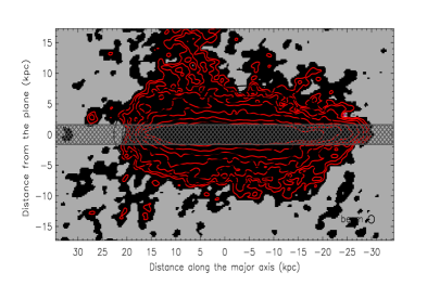
Figure 1: Total H i emission map of NGC 891 as obtained by the observations (red contours and colour scale) and by the cloud density distribution of Section 3.2 (black contours). The map has a spatial resolution of 25″($\sim 1.2$ kpc) with contour levels, starting from the outermost, of 0.15, 0.3, 0.6, 1.2, 2.4, 4.8, 9.6 $\times 10^{20}\,\rm{cm}^{-2}$. The shaded area delimits the emission expected from the disc.

3.1 The galaxy model

For the determination of the gravitational potential of NGC 891 we consider the maximum-light mass model of Fraternali & Binney (2006). This mass model consists of four distinct components: two exponential discs (stellar and gaseous), a bulge and a dark-matter halo. The volume density of the two disc components is given by

$$\rho(R,z)=\displaystyle\rho_{0}{\rm e}^{-R/R_{\rm d}}\,{\rm sech}^{2}\left(\frac{z}{h_{\rm d}}\right)\,,$$ (13)

where $\rho_{0}$ is the central density, and the dimensional constant $R_{d}$ and $h_{d}$ are, respectively, the scale-length and the scale-height of the disc. The bulge and the dark halo components are modelled using the double power-law spheroidal density profile (Dehnen & Binney 1998)

$$\rho(m)=\displaystyle\frac{\rho_{0}}{(m/a)^{\alpha}\,(1+m/a)^{\beta-\alpha}}\,,$$ (14)

where

$$m^{2}=\displaystyle R^{2}+\frac{z^{2}}{1-e^{2}}\,,$$ (15)

$e$ is the eccentricity of the spheroid, $\alpha$ and $\beta$ are the inner and outer slopes, and $a$ is the scale-length. The adopted values of the parameters to reproduce the rotation curve in the plane of NGC 891 are reported in Table 1 of Fraternali & Binney (2006), where the derivation of this potential and other mass models compatible with this rotation curve are also discussed.

3.2 The cloud distribution

A proper Jeans-based analysis of baroclinic fluid solutions requires the choice of a cloud density distribution similar to that observed. For the cloud density distribution we adopt the function

$$\rho(R,z)=\displaystyle\rho_{0}\left(1+\frac{R}{R_{{\rm g}}}\right)^{\gamma}{\rm e}^{-R/R_{{\rm g}}}\,{\rm sech}^{2}\left(\frac{z}{h_{\rm g}}\right)\,,$$ (16)

which is similar to that adopted by Oosterloo et al. (2007). In the equation above $\rho_{0}$ is the central density, $\gamma\geq 0$, $R_{{\rm g}}$ is the scale-length and the scale-height $h_{g}$ depends upon $R$ as

$$h_{\rm g}(R)=h_{0}+\displaystyle\left(\frac{R}{h_{R}}\right)^{\delta},\;\,\delta\geq 0.$$ (17)

The parameters of the distribution, excluded the central density $\rho_{0}$, are chosen is such a way that the function reproduces the H i total map shown in Fig. 1 and their values are: $R_{{\rm g}}=1.61$ kpc, $\gamma=4.87$, $h_{0}=2.3$ kpc, $\delta=2.25$ and $h_{R}=18.03$ kpc. The central density $\rho_{0}=6.63\times 10^{-4}{\rm cm}^{-3}$ is such that the total mass of the cloud system is that derived by the total H i emission; the corresponding halo mass (i.e. the mass computed for $|z|\geq 1$ kpc) of $1.13\times 10^{9}{\rm M}\odot$ is consistent with the value given in Oosterloo et al. (2007).

We now verify that the density distribution guarantees the existence of physically acceptable solutions (i.e. $u_{\varphi}^{2}\geq 0$ everywhere). It can be easily shown that $\partial\rho/\partial z\leq 0$ for the density distribution (16), whilst the radial density profile presents, for each $z$, a maximum at some value $R_{\rm max}(z)$: the positivity of $u_{\varphi}^{2}$ is then guaranteed in the region $R\leq R_{\rm max}$, where $\partial\rho/\partial R>0$, whilst it has to be investigated in the external region, where $\partial\rho/\partial R<0$ (see Section 2.1), by numerical inspection. We found that, with the adopted parameters, the density distribution (16) produces physically acceptable solutions for all the models investigated. For what concerns the vertical velocity gradient, the considerations made in Section 2.3 are valid: in particular, we expect that the rotational velocities of the models are lower than the circular velocity (8) for $R\geq R_{\rm max}$, if the vertical velocity gradient is negative.

In our models, we are only aiming to reproduce the extra-planar gas and we therefore neglect the region where emission from the disc is expected. Such a region is covered by shaded areas in all the figures where the comparison with the data is shown (Figs. 1, 3, 5, and 6). The size of this region ($|z|<1.64$ kpc), is calculated as $\pm 3\sigma\,\times$ (spatial resolution of the data) assuming that the galactic disc i̧s perfectly co-planar. In fact the resolution of the observations (HPBW$=0.64$ kpc) is much larger than the expected intrinsic scale height of the H i disc ($100-200$ pc), i.e. the disc is not resolved. The exclusion of the disc is necessary to avoid the complication of a region where the gas is almost certainly not described by the considered Jeans equations. The implicit assumption is that, in a real galaxy, at the lower halo boundaries the velocity dispersion, induced by some (unspecified) physical process in the disc, is the same as the one provided by our density distribution (see Figs. 2 and 4). This requirement is necessary for the system to be stationary.

3.3 Construction of the model

Having fixed the galaxy gravitational field and the cloud density distribution, for each model we first compute $\sigma_{z}$ by integrating numerically eq. (3) with a finite-difference scheme. In the isotropic case we then compute the rotational field from eq. (4) using the same numerical scheme. In the anisotropic cases we can integrate eq. (6) or just use (7). The rotation velocity and the azimuthal component of the velocity dispersion are then evaluated on the numerical grid by means of eqs. (9) and (10). We verified that eqs. (6) and (7) give the same results in all explored anisotropic models.

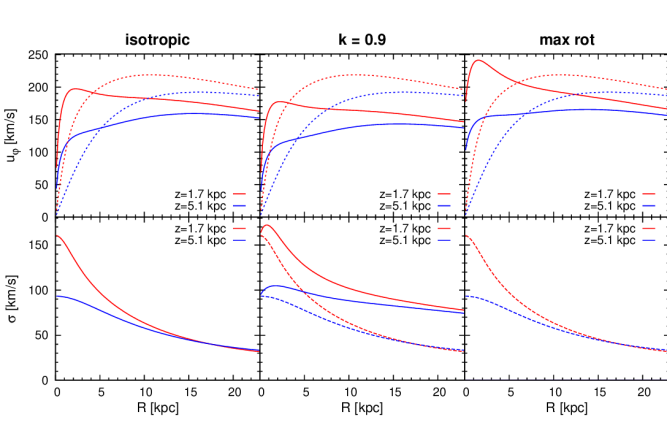
Figure 2: Intrinsic rotational velocities and velocity dispersion for system of clouds that can be described by a classical two-integral phase-space distribution function, at $z=1.7$ kpc and $z=5.1$ kpc. From left to right: isotropic model, $k=0.9$ model and maximally rotating model ($\sigma_{\varphi}=0$). Velocity panels: the dotted lines represent the circular velocity $u_{\rm c}$ whilst the solid lines are the model rotational velocities $u_{\varphi}$. Dispersion panels: the dashed lines indicate $\sigma_{z}$ and the solid lines $\sigma_{\varphi}$. In the isotropic case all the components of the dispersion are the same, whilst in the other two models $\sigma_{z}=\sigma_{R}$.

As an output for the models a pseudo-data cube, with the same spectral and spatial resolutions and total flux as the data cube of H i observations, is generated as follows. In each grid point the cloud density, the rotational velocity and the velocity dispersion are projected numerically along the line-of-sight for the inclination of the galaxy, which is assumed to be seen exactly edge-on. From the projected velocity we construct a first data cube and, to account for the effect of the velocity dispersion, we convolve the projected density in each cell of this cube with a normalised Gaussian profile with a dispersion equal to the projected velocity dispersion. Finally, for a more realistic comparison, the cube is smoothed to the same spatial resolution as the data ($FPBW=28^{{}^{\prime\prime}}\approx 1.3$ kpc). We remind that the construction of a pseudo-data cube is crucial because it bypasses all the intermediate stages of data analysis, and the assumptions made in these stages. A critical case is the comparison of the data rotation curves with the rotational velocities predicted by the models. The rotation curves of the extra-planar gas (and of edge-on galaxies in general), are usually derived by fixing a certain amount of line-of-sight velocity dispersion and using the so-called “envelope tracing” method (see Sancisi & Allen 1979; Fraternali et al. 2005). Clearly, if a model has velocity dispersions inconsistent with that adopted to derive the rotation curves from the data (as it happens here, see Section 4), a direct comparison between the two cannot be done (see Section 5).

4 Results

We now present the most important features of some of the considered stationary models for the extra-planar gas of NGC 891, and we compare them with the observations.

4.1 Isotropic model

We start by describing the main intrinsic features of the isotropic model, i.e. the analog of a stationary baroclinic fluid model where the thermal pressure of the gas is replaced by a globally isotropic velocity dispersion tensor. It is then expected that the behaviour of the isotropic model is similar to the baroclinic solutions of Barnabè et al. (2006). However, there is an important difference between these two models in the choice of the density distribution. In our model the density is chosen to match the observed H i emission (see Fig. 1), whilst the density distribution of Barnabè et al. (2006) was just chosen to satisfy the general rules that guarantee a physically acceptable rotational velocity field. In other words, our density distribution is fixed by the H i observations, and not by the requirement $u_{\varphi}^{2}\geq 0$. Using this cloud distribution the resulting $\sigma_{z}=\sigma_{R}=\sigma_{\varphi}$ has values ranging from 160 (in the centre) to $35\,{\rm km\,s^{-1}}$ (at $R\sim 20$ kpc) with mean values between 50 and $100\,{\rm km\,s^{-1}}$ (Fig. 2, bottom left panel).

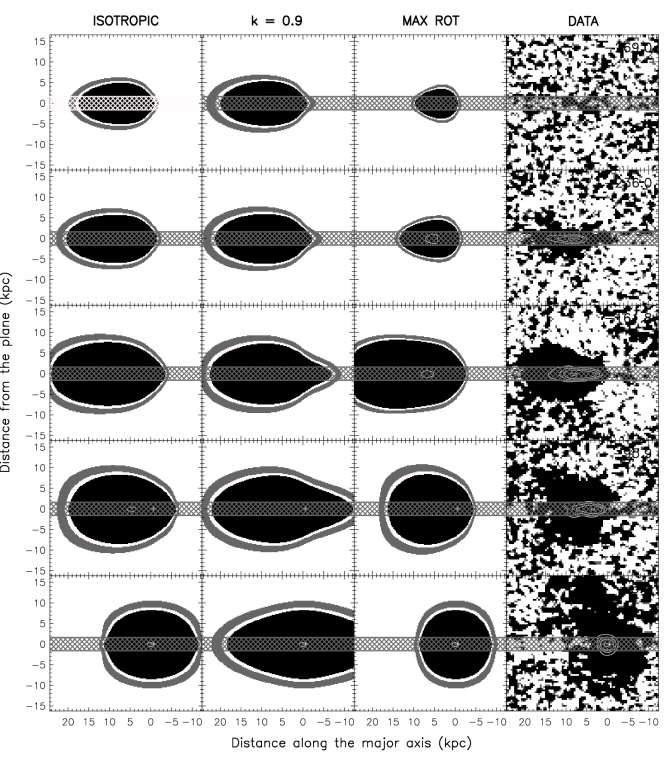
Figure 3: Comparison of representative velocity channels of the H i data cube of NGC 891 and the predictions of 3 stationary models: the isotropic (first column), the $k=0.9$ and $b=1$ (second column), and the $b=1$ maximally rotating (third column) models. The shaded area in each channel delimits the emission expected from the disc. The contour levels, starting from the outer, are 0.25, 0.5, 1, 2, 5, 10, 20, 50 mJy/beam; the beam size is 28″= 1.3 kpc.

In the left panels of Fig. 2 we present the rotation curves (top) and the radial velocity dispersion profiles (bottom) at distances from the plane $z=1.7$ kpc (lower halo boundary) and $z=5.1$ kpc; the dashed lines show the circular velocities $u_{\rm c}$. As expected from the considerations of Section 2.3, in the external regions of the galaxy the rotational velocity is below the circular velocity because of the negative vertical gradient in $u_{\varphi}$. The radial profile of the velocity dispersion shows a monotonic decrease with $R$ but the values of the dispersion are everywhere greater than the mean observed value of $\sim 20\,\rm{km\,s^{-1}}$. This latter is also the value adopted to derive the rotation curves above the plane from the H i observations of NGC 891 (Fraternali et al. 2005, here shown in Fig. 7). As a consequence, a direct comparison between these curves and the circular velocities of our models is not possible. We stress again that these problems are overcome by comparing directly the models with the raw data cubes, where all the kinematical and density effects are fully taken into account.

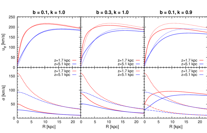
Figure 4: Intrinsic rotational velocities and velocity dispersion for the anisotropic model $b=0.1$ and $k=1$ (left column), the model $b=0.3$ and $k=1$ (central column), and the model $b=0.1$ and $k=0.9$ (right column) at $z=1.7$ kpc and $z=5.1$ kpc. Rotational velocity panels: the dotted lines represent the circular velocity $u_{\rm c}$ whilst the solid lines are the rotational velocities $u_{\varphi}$. Dispersion panels: the dashed lines indicate $\sigma_{z}$, the solid lines $\sigma_{\varphi}$ and the dashed-dotted lines $\sigma_{R}$; in the first two cases $\sigma_{\varphi}=\sigma_{R}$.

Figure 3 (first column from the left) shows the pseudo-data cube constructed from this Jeans model, while each panel in the rightmost column represents the observed emission of H i gas in a particular velocity channel. The numbers on the top right corners of the data column represent the deviations of the line-of-sight velocities from the systemic one ($528\,{\rm km}\,{\rm s^{-1}}$), whilst the shaded area on each map delimits the emission expected from the disc ($\pm 3\sigma$ spatial resolution), which we are not attempting to reproduce with this model. We can see that the observed H i emission at higher rotational velocity (corresponding to the channel at $v_{\rm los}=-236.0\,{\rm km\,s}^{-1}$) is fully due to the mid-plane, i.e. the halo is not visible. This is not surprising because the halo gas rotates more slowly than the gas in the disc and in fact, as we move towards the bottom panels, the halo emission becomes important. Due to its high velocity dispersion, in the isotropic Jeans model some emission in the halo region is present also in the upper two velocity channels; only in the middle channel the agreement is good whilst in the bottom channels the emission is too horizontally elongated.

Summarizing, it is possible to construct an isotropic Jeans model with a realistic halo density distribution, in which a negative vertical gradient in the rotational velocity is present. However, the predicted velocity dispersions along the line-of-sight are much higher than those observed, so that a number of features of the data cube are not reproduced. In order to solve these problems, in the next Section we consider different models with anisotropic velocity dispersion tensors.

4.2 Anisotropic models

The assumption of anisotropy in the velocity dispersion can overcome, at least in principle, the problems originated by the high values of $\sigma$ obtained in the isotropic models. In Section 4.2.1 we focus on the classical Satoh decomposition in a two-integral distribution function (i.e., $\sigma_{R}=\sigma_{z}$ everywhere), and in Section 4.2.2 we discuss the case of a three-integral phase-space distribution function for the cloud system. In the following, we indicate with $\sigma_{\rm los}$ the component of the velocity dispersion along the line-of-sight on each place in the galaxy.

4.2.1 Two-integral anisotropic systems

We examine here cloud systems described by a two-integral phase-space distribution function, for which $\sigma_{z}=\sigma_{R}$. The relevant equations are obtained by taking $b=1$ in eqs. (5), and adopting a Satoh decomposition in the azimuthal direction. When $k=0$ $\sigma_{\varphi}^{2}$ is maximal, while when $k=1$ the system is isotropic. Allowing for $k=k(R,z)$, more rotationally supported models can be constructed, up to the maximally rotating one where $\sigma_{\varphi}^{2}=0$ (Ciotti & Pellegrini 1996). First of all, we investigate a model with constant $k$ and we assume $k=0.9$; for lower values the disagreement with the data increases. We expect that the model is not better than the isotropic ($k=1$) case in reproducing the observations, because $\sigma_{\rm los}$ is increased by the adopted anisotropy; in particular, as can be inferred from eq. (10), $\sigma_{\varphi}\geq\sigma_{z}=\sigma_{R}$. The central column of Fig. 2 (bottom panel) clearly illustrates this fact, showing a difference among $\sigma_{\varphi}$ and the other two components of approximately $30\,{\rm km\,s^{-1}}$, on average. For what concerns the properties of the rotation curves, the considerations carried out in the isotropic case are still valid, because from eqs. (7) and (9) it follows that $u_{\varphi}=k\,u_{\rm iso}$ so that in the external regions of the galaxy $u_{\varphi}<u_{\rm c}$. The pseudo-data cube of the model presented in Fig. 3 (second column) shows that in the channels close to the systemic velocity (bottom) the emission of this model is even more elongated than in the isotropic case, in complete disagreement with the data.

Figure 5: Comparison of five representative velocity channels of the H i data cube of NGC 891 and the predictions of 3 three-integral anisotropic models: $b=0.1$ and $k=1$ (first column), $b=0.3$ and $k=1$ (second column), $b=0.1$ and $k=0.9$ (third column). The shaded area in each channel delimits the emission expected from the disc and the contour levels are the same as in Fig. 3.

In two-integral systems, the line-of-sight velocity dispersion can be reduced only if $k>1$. As a limit case, we present the results for the maximally rotating model in which $k=k_{\rm max}(R,z)\geq 1$ such that the rotational velocity has its maximum value everywhere and $\sigma_{\varphi}=0$. The corresponding intrinsic rotation curves are presented in Fig. 2 (top right panel) and their peculiarity is the steep rise in the central regions. The reduced value of $\sigma_{\rm los}$ improves the agreement with the data, as it can be seen from the pseudo-data cube of the model in Fig. 3, especially in the channels near the systemic velocity. This agreement is not so good in the channel at $v_{\rm los}=-236.0\,{\rm km\,s}^{-1}$ and in general in all the channels between $-236.0\,{\rm km\,s}^{-1}$ and $-161.8\,{\rm km\,s}^{-1}$ (not shown here) where, due to the steep rise in the rotational velocity at small $R$, there is emission in the central halo regions not seen in the data.

4.2.2 Three-integral anisotropic systems

We now turn the attention to the models with $b\leq 1$ (therefore supported by a three-integral phase-space distribution function) and we first discuss the case $\sigma_{R}=\sigma_{\varphi}$ (i.e. $k=1$). The best fit to the data is obtained by an anisotropic model with $b\sim 0.1$, which limits the line-of-sight velocity dispersion to about $20\,{\rm km\,s}^{-1}$ for a large interval of $R$ (Fig. 4, bottom left panel). The rotation curves for this model (top left panel) are very similar to the circular velocity curves, in accordance with eq. (7) which states that, in the limiting case $b=0$, the curves coincide. The pseudo-data cube of the model is presented in Fig. 5 (leftmost column). In the high velocity channels (top panels) the halo emission is still present but, at variance with the isotropic case, this is due to the fact that the rotational velocities of the model are slightly higher than those observed. In the low velocity channels (bottom panels) the halo emission is narrower than the data along the horizontal axis, due to a rapid decrease of the velocity dispersion in the outer parts. We discuss these discrepancies more in detail in Section 5.

An important issue regarding the anisotropic models is the effect that the choice of the parameters $b$ and $k$ may have on the properties of the solutions. We analyse this aspect by fixing the value of one of the two parameters and by varying the other. The results of this comparison, for representative values of $b$ and $k$, are shown in Fig. 4, where the model with $b=0.1$ and $k=1$ (which, hereafter, we will also refer to as the “high-$\sigma_{z}$ model”) has been taken as a reference case. In particular, increasing the value of $b$ at fixed $k$ has the net result of increasing the line-of-sight velocity dispersion (i.e. $\sigma_{R}$ and $\sigma_{\varphi}$) whilst the rotational velocity is decreased; the decrease in rotational velocity is also obtained when the value of $k$ is decreased at fixed $b$, but in this case only the value of $\sigma_{\varphi}$ is affected. In Fig. 5 we present the pseudo-data cubes of the models just described. The emission of the reference model ($b=0.1$, $k=1$) in all the velocity channels is less horizontally extended than that of the model with $b=0.3$, due to the smaller values of $\sigma_{\rm los}$. Although the $b=0.3$ model seems to agree better with the data in the channel maps close to systemic velocity the top panels of Fig. 5 show substantial halo emission, due to the now increased line-of-sight velocity dispersion. The interpretation of the differences between the reference model and the model with $k\neq 1$ is complicated by the fact that $\sigma_{\varphi}\neq\sigma_{R}$ so that the extension of the emission strongly depends on their relative contribution to the velocity dispersion along the line-of-sight. In particular, the importance of $\sigma_{\varphi}$ is maximum in the high velocity channels (top panels), and then it progressively diminishes in the channels near the systemic velocity in favour of $\sigma_{R}$.

In short, three-integral models with $b<1$ and $k=1$ perform better than the isotropic and the two-integral models because $\sigma_{\rm los}$ can be reduced to values comparable to the the observed one. However, a number of features of the data cubes are still not reproduced revealing intrinsic problems with all these stationary models that we discuss more in detail in the next Sections.

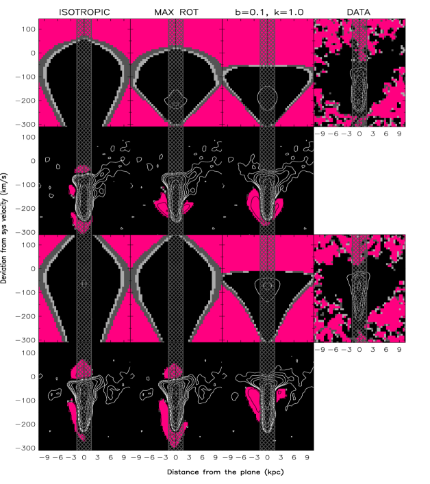
Figure 6: Comparison between two position-velocity cuts perpendicular to the plane of NGC 891 and some representative models. In the first row the cut is made at $R=7.5$ kpc on side of the galaxy where the gas is moving towards the observer, and the corresponding residuals, are presented in the second row. In the third row the cut is on the same side of the galaxy but at $R=2.8$ kpc and the residuals are shown in the fourth row. The shaded area in each plot delimits the emission expected from the disc and the contour levels are the same as in Fig. 3. For the residuals, computed subtracting the model to the data, the black contours represents positive values whilst the white contours are the negative ones; also in this case the contour levels (absolute value) are the same as in Fig. 3.

4.3 Position-velocity plots

Among the models presented above we select the three most representative and compare them further with the H i data. Figure 6 shows two cuts of data cube of NGC 891 (rightmost column) taken perpendicularly to the plane of the galaxy at $R=7.5$ kpc (first row) and $R=2.8$ kpc (third row) from the centre, towards North-East. These plots are analogous to those shown in Fig. 16 of Oosterloo et al. (2007). The position-velocity diagrams are compared with the prediction of three models: the isotropic model, the maximum rotation model and the three-integral high-$\sigma_{z}$ model. Also the corresponding residuals are shown (second and fourth rows) computed as the difference between the data and the models; the shaded area in each position-velocity plot delimits the emission expected from the disc.

The characteristic triangular shape of the data diagrams (rightmost column) is due to the negative vertical gradient in the rotational velocity of the halo and is the key feature that the models should reproduce. Clearly, this is not the case for the isotropic model as the high velocity dispersion makes the emission very elongated, although a negative vertical gradient in the rotational velocity is visible. In the $2.8$ kpc cut (third row), the emission is so elongated that a substantial amount of gas is apparently “counter-rotating” (upper part of the plot). The maximally rotating model (second column) also does not reproduce the shape of the emission especially at $R=2.8$ kpc from the centre of the galaxy (third row). Also in this case the predicted line-of sight velocity dispersion is too high. The position-velocity diagrams for the high-$\sigma_{z}$ model (third column) show a qualitative agreement with the data as the triangular shape is reproduced. However the velocity dispersion in the upper halo $|z|>5$ kpc is clearly not matched and there is a downward shift of the emission especially visible in the $7.5$ kpc cut. These features are also apparent in the residual maps and in particular the high-$\sigma_{z}$ model, despite reproducing well the shape of the data, shows substantial residuals. In addition, the residuals also reveal the intrinsic asymmetric distribution of the extra-planar gas with respect to the mid-plane of NGC 891.

Figure 6 gives a different view of the discrepancies already noted in Figs. 3 and 5. The advantage of a cut perpendicular to the plane of the galaxy is that it captures in one diagram the kinematics of the extra-planar gas at different heights and, as mentioned, its characteristic triangular shape is the evidence of the gradient in rotational velocity with height. The only model that reproduces at least qualitatively this shape is the anisotropic $b=0.1,k=1$ model.

5 Discussion

In this paper we have explored an alternative interpretation of the baroclinic fluid homogeneous models for extra-planar gas, i.e. that of a “gas” of H i clouds described by the stationary Jeans equations. Due to the formal equivalence of the equations describing the two systems, a similarity in the behaviour of the isotropic Jeans model and that of the baroclinic solutions of Barnabè et al. (2006) is expected. The present investigation is not just a re-interpretation of the results of Barnabè et al. (2006): even in the isotropic case our models differ from theirs in the choice of galaxy mass and cloud density distributions. We find that the choice of the mass model has a little impact on the properties of the solutions, but the form of the density distribution is critical. Barnabè et al. (2006) adopted a very flat density distribution, in order to reproduce the off-plane rotation curves. A flat density distribution requires less pressure support against the vertical gravitational field of the galaxy which results in a low temperature of the gas, typically $10^{5}$ K. For such a temperature the expected velocity dispersion in a Jeans isotropic model would have been of the order of $30\,\rm{km\,s^{-1}}$, close to the mean observed value (Oosterloo et al. 2007). Instead, in the present model the parameters of the density distribution are tuned to reproduce the observed H i distribution which has a greater scale-height than that used by Barnabè et al. (2006, see eq. [17]). Thus, the typical values of the velocity dispersion necessary to sustain the halo are of a factor $\sim\,$3 higher than the above. As we have seen, this high velocity dispersion has a large impact on the observable kinematics of the extra-planar gas and it is the main reason why the isotropic model fails to reproduce the data. The higher values of the velocity dispersion also influence the rotational velocities: indeed the rotation curves of our Jeans model are about $20\,\rm{km\,s^{-1}}$ lower than those obtained by Barnabè et al. (2006).

The high values of the velocity dispersion of the H i halo clouds may appear, at first sight, unphysical. However we notice that these velocities are unavoidable in any model attempting to reproduce gaseous halos with such large scale-heights (e.g. Fraternali & Binney 2006). The source of kinetic energy for these clouds must come from supernovae, indeed hydrodynamical simulations of superbubble expansion in galactic discs predict these kinds of blowout velocities (e.g. Mac Low & McCray 1988). Finally, we also notice that velocities of the order of $100\,{\rm km\,s}^{-1}$ are in fact typical for halo clouds in the Milky Way (Wakker & van Woerden 1997) and have been observed in external galaxies whenever the inclination of the disc along the line-of-sight is favorable (e.g. van der Hulst & Sancisi 1988; Boomsma et al. 2008).

As already mentioned in Sect. 4.3, the most satisfactory model is the anisotropic $b=0.1$, $k=1$ model (or high-$\sigma_{z}$ model), which has been constructed in order to have $\sigma_{R}=\sigma_{\varphi}<\sigma_{z}$. These requirements are roughly in agreement with the prescriptions for a galactic fountain where the material is ejected mostly vertically from the disc and falls back also vertically. Fraternali & Binney (2006, 2008) have build galactic fountain models for NGC 891 and compared them with the data cube in the same way we did here. They found that the halo gas distribution is well reproduced by fountain clouds that are kicked out of the disc with a Gaussian distribution of initial velocities and dispersion of about $80\,{\rm km\,s}^{-1}$, which is a value very similar to the average $\sigma_{z}$ predicted by our stationary models (Fig. 4). Moreover, Fraternali & Binney (2006) investigated the opening angles about the normal to the plane of the ejected clouds finding that it has to be lower than 15 degrees, in other words the clouds are ejected almost vertically. Therefore, the $b=0.1,k=1$ model is quantitatively similar to the fountain models. What makes the difference between the two is the lack of non-circular (inflow and outflow) ordered motions in our stationary model that, instead, in fountain models are always present.

The most problematic discrepancy between the high-$\sigma_{z}$ model and the data is visible in the channel map close to the systemic velocity (see channel at $-5.2\,{\rm km\,s}^{-1}$ in Fig. 5). This map shows the gas that has a null velocity component along the line-of-sight (once the systemic velocity has been removed). Much of this gas is located in the outer parts (in $R$) of the galaxy both in the disc and in the halo. The width of the channel (along the horizontal axis) is mostly due to the velocity dispersion of this gas. The high-$\sigma_{z}$ model fails to reproduce the data in two ways: 1) the channel map is too narrow, 2) the width (in the $x$-axis) of the emission decreases with height contrary to what seen in the data. These differences are caused by the fact that the velocity dispersion in the model decreases both with $R$ and with $z$, whilst in the data the two behaviours seem reverse. The fact that the velocity dispersion increases with height has been clearly shown by Oosterloo et al. (2007) who built artificial cubes with different parameters and compared them with the NGC 891 data cubes. These authors also kept the dispersion constant with $R$ and reproduced much better the shape of the channel maps close to the systemic velocity (see their Fig. 14). The decrease of the velocity dispersion with $R$ and $z$ is a common problem of all our stationary models and may be related to the lack of (ordered) non-circular motions mentioned above.

In the high-$\sigma_{z}$ model the rotational velocities can be directly compared with those obtained from the data because the line-of-sight velocity dispersion has values comparable with the observed one. In Fig. 7 we show the rotation curves of NGC 891 at distances from the plane of 3.9 kpc (top panel) and 5.2 kpc (from Fraternali et al. 2005). The rotational velocities predicted by the $b=0.1,k=1$ model are shown as solid lines, the dashed line shows the rotation curve in the plane. In the derivation of these rotation curves from the data, it has been assumed a constant value of the velocity dispersion ($20\,\rm{km\,s^{-1}}$). The curves have been derived using the envelope tracing method, which is such that the larger is the velocity dispersion one assumes the lower is the obtained rotational velocity. In our high-$\sigma_{z}$ model the velocity dispersion is not constant along $R$ and it is exactly $20\,{\rm km\,s}^{-1}$ only at $\sim 10$ kpc (Fig. 4). Ideally one should correct the data points for this effect obtaining slightly lower velocities for $R<10$ kpc and higher for $R>10$ kpc but the effect is minimal. Overall, for what concerns the rotation curves of NGC 891 we can say that the high-$\sigma_{z}$ stationary model predicts a gradient that is quite close to (although slightly lower than) the observed one.

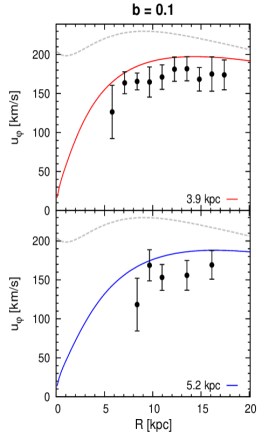
Figure 7: Rotational velocities of the model $b=0.1$ and $k=1$ (solid line) and rotation curves in the H i by Fraternali et al. (2005) (points with error bars) at $z=3.9$ kpc (top) and $z=5.2$ kpc (bottom). For each plot the long-dashed line represents the rotational velocity on the mid-plane.

The stationary models presented here do not aim to explain the origin of the extra-planar gas. Instead their goal is to find a stationary description for the extra-planar gas phenomenon whatever physical mechanism is producing it, assuming that it can be considered roughly stationary. This assumption should be reasonably valid if the extra-planar gas is produced for instance by a galactic fountain and the star formation rate of the galaxy does not vary considerably with time as it seems to be the case for galaxies like the Milky Way (e.g. Twarog 1980). The investigation presented by Fraternali & Binney (2006) shows that the rotational velocities predicted by a galactic fountain model are systematically higher than the one derived from the data and also higher than those predicted by the stationary high-$\sigma_{z}$ model shown in Fig. 7. This latter result is not surprising given that in the fountain model the gas clouds move outwards for a large fraction of their trajectories and thus tend to be at ${\rm v}_{\varphi}>u_{\rm c}$ for most of their time ($u_{\rm c}$ is the circular speed at that position). On the contrary, in the high-$\sigma_{z}$ model the gas has basically ${u}_{\varphi}\simeq u_{\rm c}$ (Fig. 4). Fraternali & Binney (2008) revised the fountain model by including interactions of the fountain clouds with the surrounding ambient medium (see also Barnabè et al. 2006 for a similar suggestion). These interactions cause the fountain clouds to lose part of their angular momentum and to decrease their rotation velocities. Such a model is to date the best description for the dynamics of the extra-planar gas. In addition to the rotational velocities, this latter model reproduces the data cube in detail including the channel maps close to the systemic velocity (see Fig. 2 of Fraternali & Binney 2008). Kaufmann et al. (2006) also reproduced the rotation curves of NGC 891 fairly well with a model in which the extraplanar gas forms by condensation of the extended warm-hot corona, but they did not attempt to build pseudo-data cubes to compare directly with the observations. However, the thermal instability on which such a model is based is unlikely to occur in galactic coronae, because of the combined effect of buoyancy and thermal conduction (Binney, Nipoti & Fraternali 2009).

Whatever the origin of the extra-planar gas, it is important to investigate whether or not it is in a stationary state. If so, it should be possible to find stationary models that reproduce these data in detail. This paper has been the second attempt of this sort after Barnabé et al. (2006). In both these attempts non-circular motions of the gas clouds have been neglected for simplicity, but in the kinematics of the extra-planar gas this kind of motions are clearly present (e.g. Boomsma et al. 2008; Fraternali et al. 2001) and they could affect substantially the observed kinematics of the halo. More likely, the cause of the discrepancy between our treatment and the observations lies on the assumptions of a Jeans-based model and in particular on the ballistic nature of the cloud motion. Not only the drag between the H i halo clouds and the corona may have an important dynamical effect but also at the turbulent cloud/corona interface there may be a considerable exchange of mass. Modelling this interface is a very challenging numerical problem (e.g. Vieser & Hensler 2007 a,b) and a secure estimate of the rate of mass exchange is not yet available. This issue will be studied in a forthcoming paper (Marinacci et al., in prep.).

6 Summary and conclusions

In this paper, motivated by the results of Barnabè et al. (2006), we investigated the possibility that the extra-planar gas in spiral galaxies can be modelled as a “gas” composed by cold H i clouds that follows the stationary Jeans equations. In doing this we are assuming that the pressure-bound clouds are moving almost ballistically in the halo. This assumption is valid in the limit of massive clouds having negligible rates of mass exchange with the corona.

In this alternative interpretation of fluid baroclinic models the thermal pressure is replaced by an isotropic velocity dispersion tensor, so that the problem of high temperature of gaseous homogeneous models is eliminated. We have also extended the discussion to simple phenomenological models with anisotropic velocity dispersion tensors. We constructed both isotropic and anisotropic models in the well-constrained gravitational field of the spiral galaxy NGC 891, and compared their predictions to the observed kinematics of the extra-planar gas in that galaxy. For each model we built a pseudo-data cube with the same resolution and total flux as the observations. The main results of our analysis can be summarized as follows:

1. The adopted functional form of the cloud density distribution, taken by the observations, leads to physically acceptable solutions in all the models investigated. The cloud density distribution is centrally depressed, and, in order to match the vertical extension of the H i halo of NGC 891, it has higher scale-height than that used by Barnabè et al. (2006).

2. All the models computed show a negative vertical gradient in the rotational velocity, the distinctive feature of the kinematics of the extra-planar gas.

3. The support against the vertical gravitational field of the galaxy requires a $\sigma_{z}\simeq 50-100\,\rm{km\,s^{-1}}$ and therefore the line-of-sight velocity dispersion of the isotropic model is a factor $\sim\,3-4$ higher than that observed.

4. With the introduction of the anisotropy it is possible to restrict the line-of-sight velocity dispersion to the observed values, but the predicted vertical gradient in the rotational velocity is somewhat too shallow and other features of the data cube are not fully reproduced.

We conclude that the dynamics of extra-planar gas in a galaxy like NGC 891 is not fully described by any of the stationary models considered here. However a model with an anisotropic velocity dispersion tensor, which mimics a galactic fountain is the preferable among all. The fact that none of the stationary Jeans models analysed here can reproduce all the features of the observed (extra-planar) gas kinematics might suggest that the cloud motion is not purely ballistic, and that the interaction between the clouds and the coronal gas, perhaps in the form of mass exchange, plays an important dynamical role.

References

- [2005] Barnabè M., Ciotti L., Fraternali F., Sancisi R., 2006, A&A, 446, 61
- [2002] Benjamin R. A., 2002, in Seeing Through the Dust: the Detection of \textH i and the Exploration of the ISM in Galaxies, ed. A. R. Taylor, T. L. Landecker & A. G. Willis (San Francisco: ASP), ASP Conf. Ser., 276, 201
- [2005] Binney J., 2005, in Extra-planar Gas Conference, ed. R. Braun, ASP Conf. Ser., 331, 131
- [2009] Binney J., Nipoti C., Fraternali F., 2009, MNRAS, 397, 1804
- [2008] Binney J., Tremaine S., 2008, Galactic Dynamics 2nd Edition (Princeton University Press, Princeton)
- [2008] Boomsma R., Oosterloo T., Fraternali F., van der Hulst J. M., Sancisi R., 2008, A&A, 490, 555
- [1980] Bregman J. N., 1980, ApJ, 236, 577
- [2000] Brüns C., Kerp J., Kalberla P. M. W., Mebold U., 2000, A&A, 357, 120
- [2008] Cappellari M., 2008, MNRAS, 390, 71
- [1996] Ciotti L., Pellegrini S., 1996, MNRAS, 279, 240
- [2002] Collins J. A., Benjamin R. A., Rand R. J., 2002, ApJ, 578, 98
- [1998] Dehnen W., Binney J., 1998, MNRAS, 294, 429
- [2008] Fraternali F., 2008, ArXiv e-prints, 0807.3365
- [2006] Fraternali F., Binney J., 2006, MNRAS, 366, 449
- [2008] Fraternali F., Binney J., 2008, MNRAS, 386, 935
- [2001] Fraternali F., Oosterloo T., Sancisi R., van Moorsel G., 2001, ApJ, 562, 47
- [2005] Fraternali F., Oosterloo T., Sancisi R., Swaters R., 2005, in Extra-planar Gas Conference, ed. R. Braun, ASP Conf. Ser., 331, 239
- [2007] Heald G. H., Rand R. J., Benjamin R. A., Bershady M. A., 2007, ApJ, 663, 933
- [2006] Kaufmann T., Mayer L., Wadsley J., Stadel J., Moore B., 2006, MNRAS, 370, 1612
- [2008] Koyama H., Ostriker E. C., 2008, ApJ, 693, 1346
- [1967] Lebovitz N. R., 1967, ARA&A, 5, 465
- [maclow] ac Low M.-M., McCray R., 1988, ApJ, 324, 776
- [1977] McKee C. F., Ostriker J. P., 1977, ApJ, 218, 148
- [2008] Melioli C., Brighenti F., D’Ercole A., de Gouveia Dal Pino E. M., 2008, MNRAS, 388, 573
- [1970] Oort J. H., 1970, A&A, 7, 381
- [2007] Oosterloo T., Fraternali F., Sancisi R., 2007, AJ, 134, 1019
- [2000] Rand R. J., 2000, ApJ, 537, L13
- [2004] Rossa J., Dettmar R.-J., Walterbros R. A. M., Norman C. A., 2004, AJ, 128, 674
- [1980] Satoh C., 1980, PASJ, 32, 41
- [2003] Sembach K. R., Wakker B. P., Savage B. D., Richter P., Meade M., Shull J. M., Jenkins E. B., Sonneborn G., Moos H. W., 2003, ApJS, 146, 165
- [1976] Shapiro P. R., Field G. B., 1976, ApJ, 205, 762
- [1975] Spitzer L. Jr., 1956, ApJ, 124, 20
- [2004] Strickland D. K., Heckman T. M., Colbert E. J. M., Hoopes C. G., Weaver K. A., 2004, ApJS, 151, 193
- [1997] Swaters R. A., Sancisi R., van der Hulst J. M., 1997, ApJ, 491, 140
- [1980] Tassoul J.-L., 1978, Theory of Rotating Stars (Princeton: Princeton University Press)
- [2004] Thilker D. A., Braun R., Walterbos R. A. M., Corbelli E., Lockman F. J., Murphy E., Maddalena R., 2004, ApJ, 601, L39
- [1980] Twarog B. A., 1980, ApJ, 242, 242
- [1988] van der Hulst T., Sancisi R., 1988, AJ, 95, 1354
- [2007a] Vieser W., Hensler G., 2007a, A&A, 472, 141
- [2007b] Vieser W., Hensler G., 2007b, A&A, 475, 251
- [wakker97] Wakker B. P., van Woerden H., 1997, ARA&A, 35, 217
- [2008] Wakker B. P., York D. G., Wilhelm R., Barentine J. C., Richter P., Beers T. C., Ivezić Ž., Howk J. C., 2008, ApJ, 672, 298
- [2001] Wang Q. D., Immler S., Walterbros R., Lauroesch J. T., Breitschwerdt D., 2001, ApJ, 555, L99
- [1978] Waxman A. M., 1978, ApJ, 222, 61
- [1995] Wolfire M. G., McKee C. F., Hollenbach D., Tielens A. G. G. M., 1995, ApJ, 453, 673