Saturation in nuclei

Abstract

This talk discusses some recent studies of gluon saturation in nuclei. We stress the connection between the initial condition in heavy ion collisions and observables in deep inelastic scattering (DIS). The dominant degree of freedom in the small $x$ nuclear wavefunction is a nonperturbatively strong classical gluon field, which determines the initial condition for the glasma fields in the initial stages of a heavy ion collision. A correlator of Wilson lines from the same classical fields, known as the dipole cross section, can be used to compute many inclusive and exclusive observables in DIS.

1 Connection between small $x$ DIS and HIC: Wilson line

The initial condition in a heavy ion collision (HIC) is determined by the wavefunctions of the two colliding nuclei, parametrized by $Q^{2}$ and $x$. As in any hadronic collision, the typical magnitudes of these parameters can be estimated as $Q^{2}\sim\langle p_{\perp}\rangle^{2}$ and $x\sim\langle p_{\perp}\rangle/\sqrt{s}$, where $\langle p_{\perp}\rangle$ is the typical transverse momentum of the particles being produced, and $\sqrt{s}$ is the collision energy. At relativistic energies, such as at RHIC and LHC, this means that the relevant domain for bulk particle production is at very small $x$. Gluon brehmsstrahlung processes lead to an exponentially (in rapidity $y=\ln 1/x$) growing cascade of gluons in the wavefunction. The number of gluons in the wavefunction grows as $\,\mathrm{d}N/\,\mathrm{d}y\sim x^{-\lambda}$, where the phenomenologically observed value is $\lambda\sim 0.2\dots 0.3$. When the number of gluons grows large enough, eventually their phase space density becomes large, with occupation numbers $\sim 1/\alpha_{\mathrm{s}}$; in terms of the field strength this meas $A_{\mu}\sim 1/g$. At this point the nonlinear terms in the QCD Lagrangian (think of the two terms in the covariant derivative $\partial_{\mu}+igA_{\mu}$) become of the same order as the linear ones, and the dynamics becomes nonperturbative. Due to the nonlinear interactions the gluon number cannot grow indefinitely, but it must saturate at some $1/\alpha_{\mathrm{s}}$ for gluons with $p_{\perp}\lesssim Q_{\mathrm{s}}$, where $Q_{\mathrm{s}}$ is the saturation scale. When $Q_{\mathrm{s}}^{2}\sim x^{-\lambda}$ becomes large enough, $\alpha_{\mathrm{s}}(Q_{\mathrm{s}})\ll 1$ and the dynamics of these fields is classical. This situation is most conveniently described using the effective theory known as the Color Glass Condensate (CGC, [1, *Weigert:2005us]), where the large $x$ degrees of freedom are described as a classical color current $J^{\mu}$ and the small $x$ gluons as classical fields that this current radiates: $[D_{\mu},F^{\mu\nu}]=J^{\nu}$.

Let us consider a hadron or a nucleus moving in the $+z$-direction. Its color current in the CGC formalism has only one large component, the one in the $+$-direction (recall that $x^{\pm}=(t\pm z)/\sqrt{2}$). For a nucleus moving at high energy we can take the current to be independent of the light cone time $x^{-}$ as $J^{+}=\rho(\mathbf{x}_{T},x^{-})$ with a very narrow, $\delta$-functionlike support in $x^{-}$: $\rho(\mathbf{x}_{T},x^{-})\sim\delta(x^{-})\rho(\mathbf{x}_{T})$. A simple solution for the equations of motion can be found as $A^{+}=\rho(\mathbf{x}_{T},x^{-})/\boldsymbol{\nabla}_{T}^{2}$; this is known as the covariant gauge solution. In order to have a physical partonic picture of the gluonic degrees of freedom it is necessary to gauge transform this solution to the light cone gauge $A^{+}=0$. The gauge transformation that achieves this is done with the Wilson line constructed from this gauge field:

$$U(\mathbf{x}_{T})=\mathbb{P}\exp\left[i\int\,\mathrm{d}x^{-}A^{+}\right].$$ (1)

This results in a field with only transverse components:

$$A^{i}_{\textnormal{(1,2)}}=\frac{i}{g}U_{\textnormal{(1,2)}}(\mathbf{x}_{T})\partial_{i}U_{\textnormal{(1,2)}}^{\dagger}(\mathbf{x}_{T})$$ (2)

for both of the colliding nuclei $(1,2)$ separately. The intial condition for the “glasma” [3] fields at $\tau>0$ is given in terms of these pure gauges [4, *Kovner:1995ja].

$$\left.A^{i}\right|_{\tau=0} = A^{i}_{\textnormal{(1)}}+A^{i}_{\textnormal{(2)}}$$ (3)

$$\left.A^{\eta}\right|_{\tau=0} = \frac{ig}{2}[A^{i}_{\textnormal{(1)}},A^{i}_{\textnormal{(2)}}]$$

Inside the future light cone $\tau>0$ the field equations must be solved either numerically or in some approximation scheme. The spacetime structure described here is illustrated in Fig. 1 (left). In the rest of this talk we shall be referring to the numerical “CYM” (Classical Yang-Mills) computations [6, *Lappi:2003bi, *Krasnitz:2003jw].

 

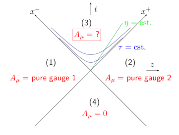
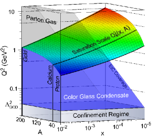
Figure 1: Left: Spacetime structure of the field. In regions (1) and (2) there is a transverse pure gauge field (2) with no energy density. In region (3) after the collision there is the glasma field. Right:

To see the connection to DIS it is convenient to consider the process in a Lorentz frame where the virtual photon has a large longitudinal momentum. In the target rest frame (or more properly the “dipole frame” [9] that does not leave all the high energy evolution in the probe) the timescales of the quantum fluctuations of the virtual photon are extremely slow. In order to interact with a hadronic target it must therefore split into a quark-antiquark pair already long before the scattering. This $q\bar{q}$-dipole then interacts with the hadronic target with a scattering amplitude whose imagimary part is known as the “dipole cross section”. As typical hadronic scattering amplitudes at high energy, that of the dipole is almost purely imaginary, and we shall here neglect the real part. The dipole cross section can be obtained from the quark propagator in the gluonic background field of the target, which is quite naturally given by the same Wilson line (1) [10]. The dipole cross section (which, in general, is a function of the size of the dipole $\mathbf{r}_{T}$, the impact parameter $\mathbf{b}_{T}$ and $x$) is the correlator of two Wilson lines

$$\hat{\sigma}(\mathbf{r}_{T})=\int\,\mathrm{d}^{2}\mathbf{b}_{T}\frac{1}{{N_{\mathrm{c}}}}\left\langle 1-U^{\dagger}\left(\mathbf{b}_{T}+\frac{\mathbf{r}_{T}}{2}\right)U\left(\mathbf{b}_{T}-\frac{\mathbf{r}_{T}}{2}\right)\right\rangle.$$ (4)

For example, the total virtual photon cross section can be obtained by convoluting the dipole cross section with the virtual photon wavefunction which relates the $Q^{2}$ of the photon to the size of the dipole $r\sim 1/Q$:

$$\sigma^{\gamma^{*}p}_{L,T}=\int\,\mathrm{d}^{2}\mathbf{b}_{T}\int\,\mathrm{d}^{2}\mathbf{r}_{T}\int\,\mathrm{d}z\left|\Psi^{\gamma}_{L,T}(Q^{2},\mathbf{r}_{T},z)\right|^{2}\sigma_{\mathrm{dip}}(x,\mathbf{r}_{T},\mathbf{b}_{T}).$$ (5)

Fourier-transforming instead of simply integrating over the impact parameter dependence gives access to the momentum transfer to the target in diffractive scattering. The inclusive diffractive virtual photon cross section (really the elastic dipole-photon cross section) is proportional to the square of the dipole cross section

$$\frac{\sigma^{D,tot}_{L,T}}{\,\mathrm{d}t}=\frac{1}{16\pi}\int\,\mathrm{d}^{2}\mathbf{r}_{T}\int\,\mathrm{d}z\left|\Psi^{\gamma}_{L,T}(Q^{2},\mathbf{r}_{T},z)\right|^{2}\sigma^{2}_{\mathrm{dip}}(x,\mathbf{r}_{T},\boldsymbol{\Delta})$$ (6)

and diffractive vector meson production can be obtained by projecting on the virtual photon wavefunction

$$\frac{\sigma^{D,V}_{L,T}}{\,\mathrm{d}t}=\frac{1}{16\pi}\left|\int\,\mathrm{d}^{2}\mathbf{r}_{T}\int\,\mathrm{d}z\left(\Psi^{\gamma}{\Psi^{*}}^{V}\right)_{L,T}(Q^{2},\mathbf{r}_{T},z)\sigma_{\mathrm{dip}}(x,\mathbf{r}_{T},\boldsymbol{\Delta})\right|^{2}.$$ (7)

The exclusive cross sections are proportional to the dipole cross section (the scattering amplitude) squared, whereas the inclusive one depends on it linearly; this is due to the optical theorem and our approximation that the scattering amplitude is purely imaginary. We shall now go on to discuss some recent applications of saturation ideas to heavy ion collisions and DIS phenomenology, trying to stress the unity of the approach between the two.

 

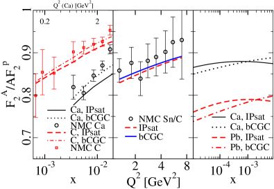
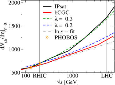
Figure 2: Left: Comparison of the fit [11] to existing nuclear DIS data from NMC. Right: Extrapolation of the gluon multiplicity to LHC energies, from [12]

2 Gluon multiplicity at RHIC and LHC AA collisions

Ideally one would like to measure the value of $Q_{\mathrm{s}}$ in DIS experiments and use the resulting value as an independent input in calculations of the initial state of heavy ion collisions. In practice most of the exiting CYM computations of the glasma fields have been performed in the MV model [13, *McLerran:1994ka, *McLerran:1994vd] in terms of the color charge density parameter $g^{2}\mu$ that parametrizes the fluctuations of the classical color currents $J^{\pm}$. One must therefore relate the values of $g^{2}\mu$ and $Q_{\mathrm{s}}$ in a consistent way. In practive this can be done by computing the Wilson line correlator in the MV model, using exactly the same numerical implementation of the model as in the CYM calculations, and extracting the correlation length $1/Q_{\mathrm{s}}$ [16].

The other ingredient necessary in using the existing DIS data to calculate initial conditions for heavy ion collisions is the correct implementation of the nuclear geometry in extending the parametrization from protons to nuclei. In a “Glauber”-like formulation of essentially independent scatterings of the dipole on each of the nucleons this is a straightforward estimate, see e.g. Refs. [11, 17]. A simple geometrical argument would give the estimate $Q_{\mathrm{sA}}^{2}\approx 0.5Q_{\mathrm{s}p}^{2}A^{1/3}$, where the coefficient in front follows from the internucleon distance in a nucleus being smaller than the nucleon radius. The actual values in the estimate of Ref. [11] are shown in Fig. 1 (right). For other estimates of $Q_{\mathrm{s}}$ based on DIS data see Ref. [18, *Armesto:2004ud]. Being really consistent with high energy evolution would require some further theoretical advances, since the approximation of independent dipole-nucleon scatterings will break down during the evolution. In the infinite momentum frame this can be thought of as gluons from different nucleons starting to interact with each other.

Combining these ingredients the CYM calculations [6, *Lappi:2003bi, *Krasnitz:2003jw] of gluon production paint a fairly consistent picture of gluon production at RHIC energies. The estimated value $Q_{\mathrm{s}}\approx 1.2\ \textrm{GeV}$ from HERA data [11, 17] (corresponding to the MV model parameter $g^{2}\mu\approx 2.1\ \textrm{GeV}$ [16]) gives a good description of existing nuclear DIS data from the NMC collaboration, see Fig. 2 (left). The same value leads to $\frac{\,\mathrm{d}N}{\,\mathrm{d}y}\approx 1100$ gluons in the initial stage. Assuming a rapid thermalization and nearly ideal hydrodynamical evolution this is consistent with the observed $\sim 700$ charged ($\sim 1100$ total) particles produced in a unit of rapidity in central collisions.

The gluon multiplicity is, across different parametrizations, to a very good approximation proportional to $\pi R_{A}^{2}Q_{\mathrm{s}}^{2}/\alpha_{\mathrm{s}}$. Thus the predictions for LHC collisions depend mostly on the energy dependence of $Q_{\mathrm{s}}$. On this front there is perhaps more uncertainty than is generally acknowledged, the estimates for $\lambda=\,\mathrm{d}\ln Q_{\mathrm{s}}^{2}/\,\mathrm{d}\ln 1/x$ varying between $\lambda=0.29$ [20] and $\lambda=0.18$ [21] in fixed coupling fits to HERA data, with a running coupling solution of the BK equation giving something in between these values [22]. This dominates the uncertainty in predictions for the LHC multiplicity, see Fig. 2 (right).

3 Multiplicity distributions

One very recent application of the CGC framework has been computing the probability distribution of the number of gluons in the glasma [23]. The dominant contributions to multiparticle correlations come from diagrams that are disconnected for fixed sources and become connected only after averaging over the color charge configurations. In other words, the dominant correlations are those arising from resummed large logarithms of the collision energy and are present already in the initial wavefunctions of the colliding nuclei.

Working with the MV model Gaussian probability distribution

$$W[\rho]=\exp\left[-\int\,\mathrm{d}^{2}\mathbf{x}_{T}\frac{\rho^{a}(\mathbf{x}_{T})\rho^{a}(\mathbf{x}_{T})}{g^{4}\mu^{2}}\right]$$ (8)

computing the correlations in the linearized approximation is a simple combinatorial problem. The result can be expressed in terms of two parameters, the mean multiplicity $\bar{n}$, and a parameter $k$ describing the width of the distribution. The $q$’th factorial moment of the multiplicity ditribution is, to leading order in $\alpha_{\mathrm{s}}$, proportional to $2^{q}(q-1)!$. Explicitly, the connected parts of the moments $m_{q}\equiv\langle N^{q}\rangle$ are

$$m_{q} = (q-1)!\,k\left(\frac{\bar{n}}{k}\right)^{q}\textrm{ with }$$ (9)

$$k \approx \frac{({N_{\mathrm{c}}}^{2}-1)Q_{\mathrm{s}}^{2}S_{\perp}}{2\pi}$$ (10)

$$\bar{n} = f_{N}\frac{1}{\alpha_{\mathrm{s}}}Q_{\mathrm{s}}^{2}S_{\perp}.$$ (11)

These moments define a negative binomial distribution with parameters $k$ and $\bar{n}$, which has been used as a phenomenological observation in high energy hadron and nuclear collisions already for a long time [24, *Alner:1985zc, *Alner:1985rj, *Ansorge:1988fg, *Adler:2007fj, *Adare:2008ns]. In terms of the glasma flux tube picture this result has a natural interpretation. The transverse area of a typical flux tube is $1/Q_{\mathrm{s}}^{2}$, and thus there are $Q_{\mathrm{s}}^{2}S_{\perp}=N_{\textnormal{FT}}$ independent ones. Each of these radiates particles independently into ${N_{\mathrm{c}}}^{2}-1$ color states in a Bose-Einstein distribution (see e.g. [30]). A sum of $k\approx N_{\textnormal{FT}}({N_{\mathrm{c}}}^{2}-1)$ independent Bose-Einstein-distributions is precisely equivalent to a negative binomial distribution with parameter $k$.

4 Inclusive nuclear diffraction at eRHIC and LHeC

The large fraction of diffractive events observed at HERA shows that modern colliders are approaching the nonlinear regime of QCD, where gluon saturation and unitarization effects become important. It should be possible to perform the same measurements in DIS off nuclei. There are plans for several facilities capable of high energy nuclear DIS experiments, as the EIC [31] and LHeC [32] colliders. Due to the difficulty in measuring an intact recoil nucleus deflected by a small angle, diffractive eA collisions present an experimental challenge. But if they are successful, nuclear diffractive DIS (DDIS) would provide a good test of our understanding of high energy QCD. Measuring the momentum transfer $t$ in both coherent (nucleus stays intact) and incoherent (nucleus breaks up into nucleons) would enable one to go measure directly the transverse structure of the gluonic degrees of freedom [33] instead of the electric charge distribution that is measured in low energy experiments. Figure 3 (left) demonstrates some expected results from such a measurement. The diffractive structure function can be divided into different components according to the polarization state of the virtual photon and the inclusion of higner Fock states (e.g. $q\bar{q}g$ in addition to $q\bar{q}$) in the dipole wavefunction. All of these have different dependences on the impact parameter of the dipole-target collision (see Fig. 3 right), which stresses the importance of having a detailed picture of the transverse geometry of both the proton and the nucleus.

 

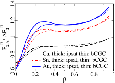
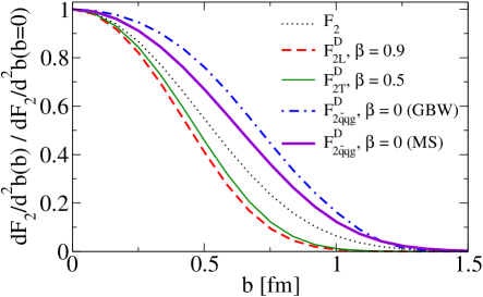
Figure 3: Left: nuclear modification of the diffractive structure function, showing characteristic suppression at small $\beta$ (large mass of the diffractive system) and enhancement at large $\beta$. From Ref. [34]. Right: dominant impact parameters for the different contributions to the proton diffractive structure function.

References

- [1] E. Iancu and R. Venugopalan, The color glass condensate and high energy scattering in QCD, in Quark gluon plasma, edited by R. Hwa and X. N. Wang, World Scientific, 2003, arXiv:hep-ph/0303204
- [2] H. Weigert, Prog. Part. Nucl. Phys. 55, 461 (2005), [arXiv:hep-ph/0501087]
- [3] T. Lappi and L. McLerran, Nucl. Phys. A772, 200 (2006), [arXiv:hep-ph/0602189]
- [4] A. Kovner, L. D. McLerran and H. Weigert, Phys. Rev. D52, 3809 (1995), [arXiv:hep-ph/9505320]
- [5] A. Kovner, L. D. McLerran and H. Weigert, Phys. Rev. D52, 6231 (1995), [arXiv:hep-ph/9502289]
- [6] A. Krasnitz, Y. Nara and R. Venugopalan, Phys. Rev. Lett. 87, 192302 (2001), [arXiv:hep-ph/0108092]
- [7] T. Lappi, Phys. Rev. C67, 054903 (2003), [arXiv:hep-ph/0303076]
- [8] A. Krasnitz, Y. Nara and R. Venugopalan, Nucl. Phys. A727, 427 (2003), [arXiv:hep-ph/0305112]
- [9] A. H. Mueller, arXiv:hep-ph/0111244
- [10] W. Buchmuller, M. F. McDermott and A. Hebecker, Nucl. Phys. B487, 283 (1997), [arXiv:hep-ph/9607290]
- [11] H. Kowalski, T. Lappi and R. Venugopalan, Phys. Rev. Lett. 100, 022303 (2008), [arXiv:0705.3047 [hep-ph]]
- [12] T. Lappi, J. Phys. G35, 104052 (2008), [arXiv:0804.2338 [hep-ph]]
- [13] L. D. McLerran and R. Venugopalan, Phys. Rev. D49, 2233 (1994), [arXiv:hep-ph/9309289]
- [14] L. D. McLerran and R. Venugopalan, Phys. Rev. D49, 3352 (1994), [arXiv:hep-ph/9311205]
- [15] L. D. McLerran and R. Venugopalan, Phys. Rev. D50, 2225 (1994), [arXiv:hep-ph/9402335]
- [16] T. Lappi, Eur. Phys. J. C55, 285 (2008), [arXiv:0711.3039 [hep-ph]]
- [17] H. Kowalski and D. Teaney, Phys. Rev. D68, 114005 (2003), [arXiv:hep-ph/0304189]
- [18] A. Freund, K. Rummukainen, H. Weigert and A. Schafer, Phys. Rev. Lett. 90, 222002 (2003), [arXiv:hep-ph/0210139]
- [19] N. Armesto, C. A. Salgado and U. A. Wiedemann, Phys. Rev. Lett. 94, 022002 (2005), [arXiv:hep-ph/0407018]
- [20] K. J. Golec-Biernat and M. Wusthoff, Phys. Rev. D59, 014017 (1999), [arXiv:hep-ph/9807513]
- [21] H. Kowalski, L. Motyka and G. Watt, Phys. Rev. D74, 074016 (2006), [arXiv:hep-ph/0606272]
- [22] J. L. Albacete, N. Armesto, J. G. Milhano, C. A. Salgado and U. A. Wiedemann, Phys. Rev. D71, 014003 (2005), [arXiv:hep-ph/0408216]
- [23] F. Gelis, T. Lappi and L. McLerran, Nucl. Phys. A828, 149 (2009), [arXiv:0905.3234 [hep-ph]]
- [24] UA1, G. Arnison et al., Phys. Lett. B123, 108 (1983)
- [25] UA5, G. J. Alner et al., Phys. Lett. B160, 193 (1985)
- [26] UA5, G. J. Alner et al., Phys. Lett. B160, 199 (1985)
- [27] UA5, R. E. Ansorge et al., Z. Phys. C37, 191 (1988)
- [28] PHENIX, S. S. Adler et al., Phys. Rev. C76, 034903 (2007), [arXiv:0704.2894 [nucl-ex]]
- [29] PHENIX, A. Adare et al., Phys. Rev. C78, 044902 (2008), [arXiv:0805.1521 [nucl-ex]]
- [30] K. Fukushima, F. Gelis and T. Lappi, arXiv:0907.4793 [hep-ph]
- [31] A. Deshpande, R. Milner, R. Venugopalan and W. Vogelsang, Ann. Rev. Nucl. Part. Sci. 55, 165 (2005), [arXiv:hep-ph/0506148]
- [32] J. B. Dainton, M. Klein, P. Newman, E. Perez and F. Willeke, JINST 1, P10001 (2006), [arXiv:hep-ex/0603016]
- [33] A. Caldwell and H. Kowalski, arXiv:0909.1254 [hep-ph]
- [34] H. Kowalski, T. Lappi, C. Marquet and R. Venugopalan, Phys. Rev. C78, 045201 (2008), [arXiv:0805.4071 [hep-ph]]