Abstract

Using dispersion relation technique and experimental data, a coupled channel analysis on $\gamma\gamma\to\pi\pi$ process is made. Di-photon coupling of $f_{0}(600)$ and $f_{0}(980)$ resonances are extracted and their dynamical properties are discussed. Especially we study the physical meaning of the coupling constant $g^{2}_{\sigma\pi\pi}$, which maintains a negative real part as determined through dispersive analyses.

1 A dispersive analysis on $\gamma\gamma\to\pi^{+}\pi^{-},\pi^{0}\pi^{0}$ processes

In recent few years there have been renewed interests on the study of the $\gamma\gamma\to\pi\pi$ process, partly due to the new experimental data provided by Belle Collaboration. [1] The investigation on such a process enables us to extract the di-photon coupling of resonances appearing in this reaction, which, as emphasized by Pennington, [2] affords a unique opportunity in exploring the underlying structure of these states. Along with previous work found in the literature, [3, 4, 5] we performed a dispersive analysis on $\gamma\gamma\to\pi^{+}\pi^{-},\pi^{0}\pi^{0}$ processes. [6] The major differences between Ref. [6] and much of previous work is that in the former we try to perform a coupled channel analysis in the strongly interacting I=0 $s$-wave – hence information from $\bar{K}K$ channel is also taken into account, at least in principle. We also fit Belle data up to 1.4GeV, which is certainly useful in fixing the $d$-waves. A better determination to the $d$-waves turns out to be very important in studying the low energy $s$-waves as well, where $d$-waves serve as a background contribution.

The dispersion representation of $\gamma\gamma\to\pi\pi,\bar{K}K$ amplitudes, $F(s)$, takes the following form: [7]

$$F(s)=F_{B}+D(s)[Ps-\frac{s^{2}}{\pi}\int_{4m_{\pi}^{2}}\frac{\mathrm{Im}D^{-1}(s^{\prime})F_{B}(s^{\prime})}{s^{\prime 2}(s^{\prime}-s-i\epsilon)}ds^{\prime}]\ ,$$ (1)

where $F_{B}$ denotes the Born term, $P$ is a two dimensional (subtraction) constant array. The $2\times 2$ matrix function $D(s)$ obeys the following equation:

$$D(s) =D(0)+\frac{s}{\pi}\int_{4m_{\pi}^{2}}\frac{D(s^{\prime})\rho(s^{\prime})T^{*}(s^{\prime})}{s^{\prime}(s^{\prime}-s-i\epsilon)}ds^{\prime}\ ,$$ (2)

where $\rho=\mathrm{diag}(\rho_{1},\rho_{2})$ and $\rho_{1}=\sqrt{1-4m_{\pi}^{2}/s}$, $\rho_{2}=\sqrt{1-4m_{K}^{2}/s}$, respectively; $T(s)$ denotes the $2\times 2$ partial wave $\pi\pi,\bar{K}K$ scattering amplitudes. Numerical solution of Eq. (2) can be searched for. In the degenerate case of single channel problem, function $D$ in Eq. (2) has a well-known analytic representation – the Omnés solution:

$$D(s)=\exp\left(\frac{s}{\pi}\int_{4m_{\pi}^{2}}^{\infty}\frac{\delta(s^{\prime})ds^{\prime}}{(s^{\prime}-s)s^{\prime}}\right)\ .$$ (3)

The $s$-wave $T$ matrix in Eq. (2) is obtained by fitting a coupled channel $K$ matrix [8] to data. [9, 10] The relevant poles are listed in table 1.

pole	sheet–II	sheet–III
$\sigma$	$0.549-0.230i$	-
$f_{0}(980)$	$0.999-0.021i$	$0.977-0.060i$ i

Table 1: The pole locations on the $\sqrt{s}$–plane, in units of GeV.

We notice from table 1 that the $f_{0}(980)$ resonance may consist of two poles – one locates on sheet II, while the other on sheet III, though the latter is found not quite stable in the numerical fit. Though the twin-pole phenomenon with respect to $f_{0}(980)$ was mentioned long time ago, [11] in $\gamma\gamma\to\pi\pi$ process one discovers further evidence in support of the idea that the $f_{0}(980)$ resonance could be a coupled channel Breit–Wigner resonance. [6] Similar phenomenon may occur in the situation of $X(3872)$ particle. [13]

The two I=0 $d$-wave and the I=2 $s$-wave amplitudes are attained through single channel approximation and the corresponding $\pi\pi$ scattering $T$ matrices are borrowed from Refs. [12, 14]. With these $T$ matrices the Omneś solution is used to determine the corresponding $D$ functions. Other partial waves are tiny and have been approximated by their Born terms. Then the $\gamma\gamma\to\pi^{+}\pi^{-},\pi^{0}\pi^{0}$ cross-sections can be fitted and the di-photon coupling of $f_{0}(600)$, $f_{0}(980)$, $f_{2}(1270)$ resonances can be extracted. We refer to Ref. [6] for the numerical results and related discussions.

By re-analyzing the whole process, the above estimates can be advanced, especially $at$ $lower$ $energies$. An improved I=0 $s$-wave single channel $\pi\pi$ scattering $T$ matrix [14] provides a better analyticity property than that of a usual $K$ matrix formalism, and gives a $\sigma$ pole location in nice agreement with the Roy equation analysis. [15] The extracted di-photon width $\Gamma(\sigma\to 2\gamma)\simeq 2.1$keV – a number significantly smaller than the value one expects for a naive $\bar{q}q$ meson. Therefore the result indicates the non-$\bar{q}q$ nature of the $f_{0}(600)$ resonance.

In the calculation as described by the last paragraph, as a byproduct when extracting the di-photon coupling one also gets the $\sigma\pi\pi$ coupling:

$$g^{2}_{\sigma\pi\pi}=(-0.20-0.13i)\mathrm{GeV}^{2}\ .$$ (4)

It could be surprising to notice that the real part of the coupling strength, $\mathrm{Re}[g^{2}_{\sigma\pi\pi}]$, is negative. A narrow resonance with such a property is not allowed, since it would be a ghost rather than a particle. In the next section we devote to the discussion on physics behind this (once again) odd property of the $f_{0}(600)$ or $\sigma$ meson.

2 What does a negative $\mathrm{Re}[g^{2}_{\sigma\pi\pi}]$ tell us?

The negative value of $\mathrm{Re}[g^{2}_{\sigma\pi\pi}]$ is related to the large width of $f_{0}(600)$ meson. To initiate the investigation let us recall the PKU dispersive representation for a partial wave elastic scattering $S$ matrix element: [14, 16]

$$S^{phy.}=\prod_{i}S^{R_{i}}\cdot S^{cut}\ ,$$ (5)

where $S^{R_{i}}$ denotes the $i$-th resonances on sheet II and $S^{cut}$ stands for the cut contribution. In each $S^{R_{i}}$ pole residue is a function of the pole location, and hence if we neglect every pole and cut contribution other than the $f_{0}(600)$ pole, we can obtain its coupling strength to two pions, $g^{2}_{\sigma\pi\pi}=({-0.18}-0.20i)\mathrm{GeV}^{2}$, which is found not much different from the value given by Eq. (4). This implies that the $\sigma\pi\pi$ coupling is mainly of a kinematical effect, $i.$ $e.$, largely affected by the $\sigma$ pole location. In Fig. 1 we draw the region where the residue contains a negative real part based on the above approximation, $i.$ $e.$, considering only single pole contribution. In the following, however, by studying the solvable $O(N)$ $\sigma$ model, we will be able to learn more lessons on physics of negative coupling strength.

The bare IJ=00 channel $\pi\pi$ scattering amplitude takes the following form: [17]

$$T^{00}\left(s\right)=\frac{1}{32\pi}\frac{s-m_{\pi}^{2}}{f_{\pi}^{2}-\left(s-m_{\pi}^{2}\right)\left({\frac{1}{\lambda}_{0}+\widetilde{B}_{0}\left(s\right)}\right)}$$

where

$$\widetilde{B}_{0}\left(p^{2}\right)=\frac{-i}{2}\int\frac{\mathrm{d}^{4}q}{\left(2\pi\right)^{4}}\frac{1}{q^{2}-m_{\pi}^{2}}\frac{1}{\left(p+q\right)^{2}-m_{\pi}^{2}}$$

is a divergent integral and can be made finite by redefining the renormalized coupling constant as, [18]

$$\frac{1}{\lambda(M)}=\frac{1}{\lambda_{0}}-\frac{i}{2}\int\frac{d^{4}q}{(2\pi)^{4}}\,\frac{1}{(q^{2}+i\epsilon)(q^{2}-M^{2}+i\epsilon)}\ ,$$ (6)

$${\frac{1}{\lambda(M)}+\tilde{B}(p^{2};M)}=\frac{1}{\lambda_{0}}+\tilde{B}_{0}(p^{2})\ ,$$

where

$$\tilde{B}(s;M)=\frac{1}{32\pi^{2}}\left[1+\rho(s)\log\frac{\rho(s)-1}{\rho(s)+1}-\log\frac{m_{\pi}^{2}}{M^{2}}\right]\ .$$

To define the theory one can set

$${1\over\lambda(M)}=0\ ,$$

where $M$ denotes the scale when perturbation expansion fails, though above the scale $M$ the theory can still be fine. The RGE of coupling constant $\lambda$ becomes exact,

$$\mu^{2}\frac{d\lambda}{d\mu^{2}}=\frac{\lambda^{2}(\mu^{2})}{32\pi^{2}}\ .$$ (7)

The true problem of such a theory (herewith called as $O(N)$ v1) is that a tachyon appears at $m_{t}^{2}$, and hence the theory only works when $|s|<<|m_{t}^{2}|$. [18]

If one does not like the tachyon a sharp momentum cutoff at $\Lambda$ can be used to make the theory finite. In this way one avoids the tachyon, but a spurious cut (at $4\Lambda^{2}$) and a spurious physical sheet pole near the spurious cut occur, instead. By this mean we define a cutoff version of the effective theory. Setting for example

$${1\over\lambda(\Lambda)}=0\ ,$$

defines another version of $O(N)$ model (called as $O(N)$ v2 hereafter).

The region where $\mathrm{Re}[g^{2}_{\sigma\pi\pi}]<0$ is plotted in Fig. 1 both for $O(N)$ model v1 and v2, which are, however, almost identical. The $\sigma$ pole trajectories with respect to varying the defining scale of two models are also plotted. Clearly, seen from Fig. 1, it is actually very difficult for $O(N)$ models to reach the ‘realistic’ $\sigma$ pole location. In model v1, one has to decrease the scale $M$ to face a situation that the tachyon pole mass and the $\sigma$ pole mass are comparable in magnitude, and hence breaks down the validity of the effective theory. In model v2 similar things happen; in order to get the $\sigma$ pole deep inside the region where $\mathrm{Re}[g^{2}_{\sigma\pi\pi}]<0$, one has to decrease the cutoff parameter $\Lambda$ facing the situation that the $\sigma$ mass is comparable in magnitude with $\Lambda$, and thus also results in breaking the validity of the effective theory. The conclusion is that QCD interaction in the scalar sector becomes so strong that, the $O(N)$ toy model even fails to handel the situation when the $\sigma$ pole gets as light and broad as it is determined from reality. A more ‘realistic’ calculation also leads to a similar conclusion. [19]

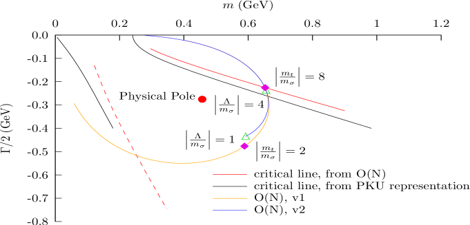
Figure 1: Region on the $\sqrt{s}$-plane with $\mathrm{Re}[g^{2}_{\sigma\pi\pi}]<0$.

Another way to look at the non-perturbative nature of the $\sigma$ meson is through examining the renormalization group equation, Eq. (7). To get the ‘realistic’ $\sigma$ pole location, one finds $\lambda(\mu)$ blows up at $\mu\simeq 0.55$MeV.

It is certainly an extremely hard and non-perturbative task to predict a pole from an effective lagrangian inside which the pole does not have a corresponding field. Such kind of poles are sometimes called as ‘dynamically generated’ resonances. Once the existence of the $\sigma$ pole was firmly established, it is wondered whether one should add the $\sigma$ field explicitly into the low energy effective lagrangian. However the blow up of the the coupling constant $\lambda$ at very low energy indicates that, even if the explicit $\sigma$ degrees of freedom is added into the effective lagrangian, one still face a strongly non-perturbative problem.

To summarize, the $\sigma$ pole manifests the maximal ‘non-perturbativity’ that QCD could offer.

This work is supported in part by National Nature Science Foundation of China under Contract Nos. 10875001, 10721063, 10647113 and 10705009.

References

- [1] T. Mori et al. (Belle Collaboration), Phys. Rev. D75(2007)051101.
- [2] M. R. Pennington, invited talk at YKIS Seminar on New Frontiers in QCD: Exotic Hadrons and Hadronic Matter, Kyoto, Japan, 20 Nov - 8 Dec 2006. Prog. Theor. Phys. Suppl. 168(2007)143.
- [3] Here we are only able to provide an incomplete list of references: D. Morgan, M. R. Pennington, Z. Phys. C48(1990)623; G. Mennessier, Z. Phys. C16 (1983) 241; A. V. Anisovich, V. V. Anisovich, Phys. Lett. B467 (1999) 289; L. V. Fil’kov, V. L. Kashevarov, Phys. Rev. C72 (2005) 035211; N. N. Achasov, G. N. Shestakov, arXive: 0712.0885 [hep-ph]; J. A. Oller, L. Roca, C. Schat, Phys. Lett. B659 (2008) 201.
- [4] J. Bernabeu, J. Prades, Phys. Rev. Lett. 100 (2008) 241804.
- [5] G. Mennessier, S. Narison, W. Ochs, Phys. Lett. B665 (2008) 205.
- [6] Y. Mao et al., Phys. Rev. D79 (2009) 116008.
- [7] O. Babelon et al., Nucl. Phys. B113(1976)445; O. Babelon et al., Nucl. Phys. B114(1976)252.
- [8] K. L. Au, D. Morgan and M. R. Pennington, Phys. Rev. D35(1987)1633.
- [9] W. Ochs, Ph.D. thesis, Munich Univ., 1974; D. H. Cohen et al., Phys. Rev. D22(1980)2595; A. Etkin et al., Phys. Rev. D25(1982)1786; A. D. Martin, E. N. Ozmutlu, Nucl. Phys. B158(1979)520; G. Costa et al., Nucl. Phys. B175(1980)402; V. A. Polychronakos et al., Phys. Rev. D19(1979)1317.
- [10] S. Pislak et al., Phys. Rev. D67(2003)072004.
- [11] Y. Fujii, M. Kato, Nuovo Cimento 13A(1973)311; D. Morgan, Nucl. Phys. A543(1992)632.
- [12] J. J. Wang, Z. Y. Zhou, H. Q. Zheng, JHEP 0512(2005)019.
- [13] O. Zhang et al., arXiv: 0901.1553 [hep-ph], to appear in PLB.
- [14] Z. Y. Zhou et al., JHEP 0502(2005)043.
- [15] I. Caprini, G. Colangelo, H. Leutwyler, Phys. Rev. Lett. 96, 132001 (2006).
- [16] Z. Y. Zhou, H. Q. Zheng, Nucl. Phys.A775(2006)212; H. Q. Zheng et al., Nucl. Phys. A733(2004)235;
- [17] S. Coleman, R. Jackiw and H. D. Politzer, Phys. Rev. D10(1974)2491.
- [18] R. Sekhar Chivkula and M. Golden, Nucl. Phys. B372(1992)44 and references therein.
- [19] M. X. Su, L. Y. Xiao, H. Q. Zheng, Nucl. Phys. A792(2007)288.