Fine-tuning favors mixed axion/axino cold dark matter
over neutralinos in the minimal supergravity model

Abstract:

Over almost all of minimal supergravity (mSUGRA or CMSSM) model parameter space, there is a large overabundance of neutralino cold dark matter (CDM). We find that the allowed regions of mSUGRA parameter space which match the measured abundance of CDM in the universe are highly fine-tuned. If instead we invoke the Peccei-Quinn-Weinberg-Wilczek solution to the strong $CP$ problem, then the SUSY CDM may consist of an axion/axino admixture with an axino mass of order the MeV scale, and where mixed axion/axino or mainly axion CDM seems preferred. In this case, fine-tuning of the relic density is typically much lower, showing that axion/axino CDM ($a\tilde{a}$CDM) is to be preferred in the paradigm model for SUSY phenomenology. For mSUGRA with $a\tilde{a}$CDM, quite different regions of parameter space are now DM-favored as compared to the case of neutralino DM. Thus, rather different SUSY signatures are expected at the LHC in the case of mSUGRA with $a\tilde{a}$CDM, as compared to mSUGRA with neutralino CDM.

1 Introduction

A wide array of astrophysical data point to us living in a universe comprised of $4\%$ baryons, $\sim 25\%$ cold dark matter (CDM) and $\sim 70\%$ dark energy. In fact, the cosmic abundance of CDM has been recently measured to high precision by the WMAP collaboration[1], which finds

$$\Omega_{CDM}h^{2}=0.110\pm 0.006,$$ (1)

where $\Omega=\rho/\rho_{c}$ is the dark matter density relative to the closure density, and $h$ is the scaled Hubble constant. No particle present in the Standard Model (SM) of particle physics has the correct properties to constitue the CDM, so some form of new physics is needed. It is compelling, however, that candidate CDM particles do emerge naturally from two theories which provide solutions to longstanding problems in particle physics.

The first problem– known as the gauge hierarchy problem– arises due to quadratic divergences in the scalar sector of the SM. These divergences lead to scalar masses blowing up to the highest scale in the theory (e.g. in grand unified theories (GUTS), the GUT scale $M_{GUT}\simeq 2\times 10^{16}$ GeV), unless an enormous fine-tuning of parameters is invoked. One solution to the gauge hierarchy problem occurs by introducing supersymmetry (SUSY) into the theory. The inclusion of softly broken SUSY leads to a cancellation of quadratic divergences between fermion and boson loops, so that only log divergences remain. The log divergence is soft enough that vastly different scales remain stable within a single effective theory. In SUSY theories, the lightest neutralino emerges as an excellent WIMP CDM candidate. Gravity-mediated SUSY breaking models (supergravity, or SUGRA) contain gravitinos with weak-scale masses. SUGRA models experience tension due to possible overproduction of gravitinos in the early universe, leading to an overabundance of CDM. In addition, gravitinos usually decay during or after Big Bang nucleosynthesis (BBN), and their energetic decay products may disrupt the successful calculations of light element abundances, which otherwise maintain good agreement with observation. This tension in SUGRA models is known as the gravitino problem.

The second problem is the strong $CP$ problem[2]. An elegant solution to the strong $CP$ problem was proposed by Peccei and Quinn (PQ) many years ago[3]. The PQ solution automatically predicts the existence of a new particle (WW)[4]: the axion $a$. While the original PQWW axion was soon ruled out, models of a nearly “invisible axion” were developed in which the PQ symmetry breaking scale was moved up to energies of order $f_{a}\sim 10^{9}-10^{12}$ GeV[5, 6]. The axion also turns out to be an excellent candidate particle for CDM in the universe[7].

Of course, it is highly desirable to simultaneously account for both the strong $CP$ problem and the gauge hierarchy problem. In this case, it is useful to invoke supersymmetric models which include the PQWW solution to the strong $CP$ problem[8]. In a SUSY context, the axion field is just one element of an axion supermultiplet. The axion supermultiplet contains a complex scalar field, whose real part is the $R$-parity even saxion field $s(x)$, and whose imaginary part is the axion field $a(x)$. The supermultiplet also contains an $R$-parity odd spin-$\frac{1}{2}$ Majorana field, the axino $\tilde{a}$[9]. The saxion, while being an $R$-parity even field, nonethless receives a SUSY breaking mass likely of order the weak scale. The axion mass is constrained by cosmology and astrophysics to lie in a favored range $10^{-2}$ eV$\stackrel{{\scriptstyle>}}{{\sim}}m_{a}\stackrel{{\scriptstyle>}}{{\sim}}10^{-5}$ eV. The axino mass is very model dependent[10, 11, 12, 13], depending heavily on the exact form of the superpotential and the mechanism for SUSY breaking. In supergravity models, it may be of order the gravitino mass $m_{3/2}\sim$ TeV, or as low as $m_{3/2}^{2}/f_{a}\sim$keV. Conditions for realizing these extremes are addressed in [12]. Here, we will try to avoid explicit model-dependence, and adopt $m_{\tilde{a}}$ as lying within the general range of keV-GeV, as in numerous previous works[11, 13, 14, 15, 16]. An axino in this mass range would likely serve as the lightest SUSY particle (LSP), and is also a good candidate particle for cold dark matter[11, 13].

In a previous paper[16], we investigated supersymmetric models wherein the PQ solution to the strong $CP$ problem is assumed. For definiteness, we restricted the analysis to examining the paradigm minimal supergravity (mSUGRA or CMSSM) model[17]. We were guided in our analysis by considering the possibility of including a viable mechanism for baryogenesis in the early universe. In order to do so, we needed to allow for re-heat temperatures after the inflationary epoch to reach values $T_{R}\stackrel{{\scriptstyle>}}{{\sim}}10^{6}$ GeV. We found that in order to sustain such high re-heat temperatures, as well as generating predominantly cold dark matter, we were pushed into mSUGRA parameter space regions that are very different from those allowed by the case of thermally produced neutralino dark matter. In addition, we found that very high values of the PQ breaking scale $f_{a}/N$ of order $10^{11}-10^{12}$ GeV were needed, leading to the mSUGRA model with mainly axion cold dark matter, but also with a small admixture of thermally produced axinos, and an even smaller component of warm axino dark matter arising from neutralino decays. The favored axino mass value is of order 100 keV. We note here recent work on models with dominant axion CDM explore the possibility that axions form a cosmic Bose-Einstein condensate, which can allow for the solution of several problems associated with large scale structure and the cosmic background radiation[18].

In this paper, we will examine the mSUGRA model under the assumption 1. of neutralino CDM and 2. that mixed axion/axino DM ($a\tilde{a}$DM) saturates the WMAP measured abundance. To compare the two DM scenarios, we will evaluate a measure of fine-tuning in the relic abundance

$$\Delta_{a_{i}}\equiv\frac{\partial\log\Omega_{DM}h^{2}}{\partial\log a_{i}}$$ (2)

with respect to variations in fundamental parameters $a_{i}$ of the model. Such a measure of relic abundance fine-tuning was previously calculated in Ref. [20] in the context of just neutralino dark matter. Here, we will expand upon this and also consider fine-tuning of the relic density in the case of mixed $a\tilde{a}$DM. Our main conclusion is that the relic abundance of DM is much less fine-tuned in the case of mixed $a\tilde{a}$CDM, as compared to neutralino CDM. Thus, we find that mixed $a\tilde{a}$CDM is theoretically preferable to neutralino CDM, at least in the case of the mSUGRA model, and probably also in many cases of SUGRA models with non-universal soft SUSY breaking terms.

We will restrict our work to cases where the lightest neutralino $\widetilde{Z}_{1}$ is either the LSP or the next-to-lightest SUSY particle (NLSP) with an axino LSP; the case with a stau NLSP and an axino LSP has recently been examined in Ref. [14]. Related previous work on axino DM in mSUGRA can be found in Ref. [15].

The remainder of this paper is organized as follows. In Sec. 2, we calculate the neutralino relic abundance fine-tuning parameter $\Delta_{\widetilde{Z}_{1}}$ in the mSUGRA model due to variation in parameters $m_{0}$ and $m_{1/2}$. We find, in good agreement with Ref. [20], that the WMAP allowed regions are all finely-tuned for low values of $\tan\beta$. For much higher $\tan\beta\sim 50$, the fine-tuning is much less with respect to $m_{0}$ and $m_{1/2}$, but nevertheless high with respect to $\tan\beta$. In Sec. 3, we review the gravitino problem, leptogenesis and the cosmological production of axion and axino dark matter. In Sec. 4, we calculate the fine-tuning parameter $\Delta_{a\tilde{a}}$ for mixed $a\tilde{a}$CDM under the assumption of a very light axino with $m_{\tilde{a}}\sim 0.1-1$ MeV. The fine-tuning is always quite low, for both cases of mixed axino/axion CDM and mainly axion CDM. In the case of mainly axino CDM, we find the scenario less well-motivated since for high values of $T_{R}\stackrel{{\scriptstyle>}}{{\sim}}10^{6}$ GeV, the value of $m_{\tilde{a}}\ll 0.1$ MeV, making the axino mainly warm DM instead of cold DM. In Sec. 5, we present a summary and conclusions.

2 Fine-tuning in mSUGRA with neutralino cold dark matter

2.1 Overview

We adopt the mSUGRA model[17] as a template model for examining the issue of fine-tuning in cases of neutralino CDM vs. $a\tilde{a}$CDM. The mSUGRA parameter space is given by

$$m_{0},\ m_{1/2},\ A_{0},\ \tan\beta,\ sign(\mu),$$ (3)

where $m_{0}$ is the unified soft SUSY breaking (SSB) scalar mass at the GUT scale, $m_{1/2}$ is the unified gaugino mass at $M_{GUT}$, $A_{0}$ is the unified trilinear SSB term at $M_{GUT}$ and $\tan\beta\equiv v_{u}/v_{d}$ is the ratio of Higgs field vevs at the weak scale. The GUT scale gauge and Yukawa couplings, and the SSB terms are evolved using renormalization group equations (RGEs) from $M_{GUT}$ to $m_{weak}$, at which point electroweak symmetry is broken radiatively, owing to the large top quark Yukawa coupling. At $m_{weak}$, the various sparticle and Higgs boson mass matrices are diagonalized to find the physical sparticle and Higgs boson masses. The magnitude, but not the sign, of the superpotential $\mu$ parameter is determined by the EWSB minimization conditions.

We adopt the Isasugra subprogram of Isajet to generate sparticle mass spectra[21]. Isasugra performs an iterative solution of the MSSM two-loop RGEs, and includes an RG-improved one-loop effective potential evaluation at an optimized scale, which accounts for leading two-loop effects[22]. Complete one-loop mass corrections for all sparticles and Higgs boson masses are included[23]. For the neutralino relic density, we use the IsaReD subprogram of Isajet[24].

Our measure of fine-tuning in the neutralino relic density, $\Delta_{\widetilde{Z}_{1}}$, is calculated by constructing a grid of points in $m_{0}-m_{1/2}$ space. At each point, the change in $\Omega_{\widetilde{Z}_{1}}h^{2}$ corresponding to a change in either $m_{0}$ or $m_{1/2}$ is calculated for both a positive and negative parameter change, using

$$\Delta_{a_{i}}=\frac{a_{i}}{\Omega_{\tilde{Z}_{1}}h^{2}}\frac{\partial\Omega_{\tilde{Z}_{1}}h^{2}}{\partial a_{i}}=\frac{a_{i}}{\Omega_{\tilde{Z}_{1}}h^{2}}\frac{\left[\Omega_{\tilde{Z}_{1}}h^{2}(a_{i}\pm\Delta a_{i})-\Omega_{\tilde{Z}_{1}}h^{2}(a_{i})\right]}{\Delta a_{i}}\;,$$ (4)

where $a_{i}=m_{0}$ or $m_{1/2}$. For each $a_{i}$, the largest $\Delta_{a_{i}}$ is selected from the results for both the positive and negative change. To construct the overall total $\Delta_{\widetilde{Z}_{1}}$, the individual values are added in quadrature:

$$\Delta_{\widetilde{Z}_{1}}=\sqrt{\Delta_{m_{0}}^{2}+\Delta_{m_{1/2}}^{2}}\;.$$ (5)

We may also consider fine-tuning due to variation in $A_{0}$ and $\tan\beta$. Variation in $A_{0}$ yields tiny variations in $\Omega_{\widetilde{Z}_{1}}h^{2}$ unless one moves close to the stop co-annihilation region (see Fig. 8 in Sec. 2.3). Variation in $\tan\beta$ gives a slight effect on the relic density unless $\tan\beta$ becomes very large. In this case, $m_{A}$ decreases[25] to the extent that $m_{A}\sim 2m_{\widetilde{Z}_{1}}$, and neutralino annihilation rates are greatly increased due to the $A$-resonance. Then, variation in $\tan\beta$ mainly shifts the location of the $A$-resonance in the $m_{0}\ vs.\ m_{1/2}$ plane. Moving on and off the resonance is already accounted for by varying $m_{0}$ and $m_{1/2}$. Nevertheless, in Sec. 2.3 we present results due to including $A_{0}$ and $\tan\beta$ in the fine-tuning calculation.

2.2 Results from variation of $m_{0}$ and $m_{1/2}$

Our first results are shown in Fig. 1, where we show in frame a). contours of $\Omega_{\widetilde{Z}_{1}}h^{2}$ in the $m_{0}\ vs.\ m_{1/2}$ mSUGRA plane for $A_{0}=0$, $\tan\beta=10$ and $\mu>0$. We also take $m_{t}=172.6$ GeV. The well-known red regions are excluded either due to a stau LSP (left-side) or lack of appropriate EWSB (lower and right side). The gray-shaded region is excluded by LEP2 chargino searches ($m_{\widetilde{W}_{1}}>103.5$ GeV), and the green shaded region denotes allowable points with $\Omega_{\widetilde{Z}_{1}}h^{2}\leq 0.11$. The region below the orange dashed contour is excluded by LEP2 Higgs searches, which require $m_{h}>114.4$ GeV; here, we actually require $m_{h}>111$ GeV to reflect a roughly 3 GeV error on the RGE-improved one-loop effective potential calculation of $m_{h}$.

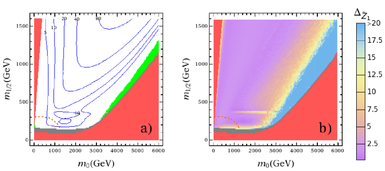
Figure 1: In the $m_{0}\ vs.\ m_{1/2}$ plane of the mSUGRA model for $A_{0}=0$, $\tan\beta=10$ and $\mu>0$, we plot a). contours of $\Omega_{\widetilde{Z}_{1}}h^{2}$ and b). regions of fine-tuning parameter $\Delta_{\widetilde{Z}_{1}}$.

The well-known (green-shaded) hyperbolic branch/focus point (HB/FP) region[26] stands out on the right side, where $\mu$ becomes small and the $\widetilde{Z}_{1}$ becomes a mixed bino-higgsino state. On the left edge, the very slight stau co-annihilation region[27] is barely visible. We also plot contours of $\Omega_{\widetilde{Z}_{1}}h^{2}$ ranging from 5 to 80. In most of the mSUGRA parameter space, the relic abundance is 1-3 orders of magnitude higher than the WMAP measured value. The valley in $\Omega_{\widetilde{Z}_{1}}h^{2}$ around $m_{1/2}\sim 400$ GeV is due to the turn-on of the $\widetilde{Z}_{1}\widetilde{Z}_{1}\rightarrow t\bar{t}$ annihilation mode.

In Fig. 2, we show the neutralino relic density as a 3-d plot in the $m_{0}\ vs.\ m_{1/2}$ plane, to gain extra perspective. The level of fine-tuning corresponds to the slope of the surface. We see that in most of parameter space, the slope is relatively small, i.e. the plateau is nearly flat. However, in this region, the relic density is far too high. In the regions where $\Omega_{\widetilde{Z}_{1}}h^{2}\sim 0.1$, then the slope is extremely steep, corresponding to large fine-tuning: a small variation in fundamental parameters leads to a large change in relic density.

Figure 2: A 3-d plot of neutralino relic density in the $m_{0}\ vs.\ m_{1/2}$ plane of the mSUGRA model for $A_{0}=0$, $\tan\beta=10$ and $\mu>0$.

In Fig. 1 b)., we show regions of fine-tuning parameter $\Delta_{\widetilde{Z}_{1}}$. A value of $\Delta_{\widetilde{Z}_{1}}\sim 0$ corresponds to no fine-tuning (a flat slope in $\Omega_{\widetilde{Z}_{1}}h^{2}$ versus variation in all parameters), while higher values of $\Delta_{\widetilde{Z}_{1}}$ give increased fine-tuning in the relic density. We see immediately from the figure that the vast majority of parameter space, where $\Omega_{\widetilde{Z}_{1}}h^{2}$ is much too large, is also not very fine-tuned. However, the HB/FP region, where $\mu\rightarrow 0$, has a very high fine-tuning, with $\Delta_{\widetilde{Z}_{1}}$ ranging from 20-100! There are also regions of substantial fine-tuning adjacent to the LEP2 chargino mass excluded region, due to rapid changes in $\Omega_{\widetilde{Z}_{1}}h^{2}$ as one approaches the $\widetilde{Z}_{1}\widetilde{Z}_{1}\rightarrow h$ annihilation resonance[28], and also some fine-tuning at the turn on of $\widetilde{Z}_{1}\widetilde{Z}_{1}\rightarrow t\bar{t}$. Finally, we see a very narrow region of fine-tuning extending along the stau co-annihilation region.

To get a better grasp, we plot in Fig. 3 a slice out of parameter space at $m_{1/2}=250$ and 500 GeV, showing in a). $\Omega_{\widetilde{Z}_{1}}h^{2}$ and in b). $\Delta_{\widetilde{Z}_{1}}$ versus $m_{0}$. We see the slope in $\Omega_{\widetilde{Z}_{1}}h^{2}$ is very steep in the HB/FP region, leading to $\Delta_{\widetilde{Z}_{1}}\sim 30$ (50) for lower (higher) $m_{1/2}$ values. In contrast, in the stau co-annihilation region, where $\Omega_{\widetilde{Z}_{1}}h^{2}\sim 0.11$, the value of $\Delta_{\widetilde{Z}_{1}}\sim 3$ (12) for low (high) $m_{1/2}$. The lower $m_{1/2}$ value has only moderate fine-tuning since it is getting close to the “bulk” annihilation region[29], where $\widetilde{Z}_{1}\widetilde{Z}_{1}$ annihilation is enhanced via light $t$-channel slepton exhange diagrams.

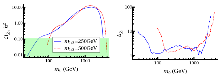
Figure 3: A plot of a). $\Omega_{\widetilde{Z}_{1}}h^{2}$ and b). $\Delta_{\widetilde{Z}_{1}}$ versus $m_{0}$ for fixed values of $m_{1/2}=250$ GeV (blue) and $m_{1/2}=500$ GeV (red), in mSUGRA with $A_{0}=0$, $\tan\beta=10$ and $\mu>0$.

To gain a better perspective on the stau co-annihilation region, in Fig. 4 we show a blown-up portrait of the low $m_{0}$ region of parameter space. The “turn-around” in the green-shaded WMAP allowed region in frame a). is due to the impact of the bulk annihilation region. Most of this area lies below the $m_{h}=111$ GeV contour, and thus gives rise to Higgs bosons that are too light. In frame b). is a blow-up of the fine-tuning parameter $\Delta_{\widetilde{Z}_{1}}$. We see that the major portion of the stau co-annihilation region is fine-tuned, with the possible exception of the region lying just below the LEP2 $m_{h}$ bound, where mixed bulk/co-annihilation occurs.

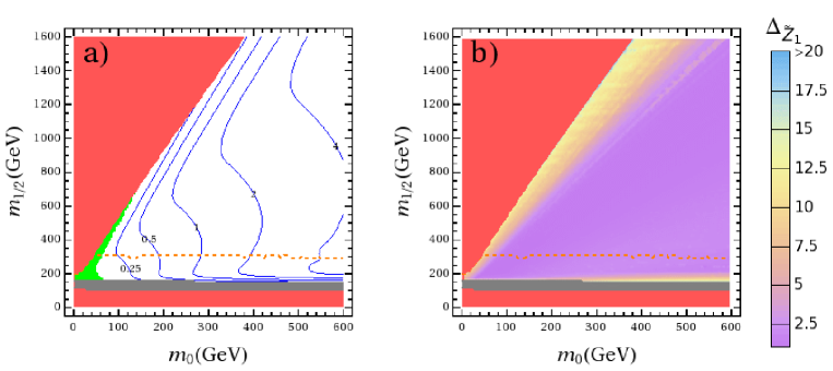
Figure 4: A plot of a). contours of $\Omega_{\widetilde{Z}_{1}}h^{2}$ and b). $\Delta_{\widetilde{Z}_{1}}$ in mSUGRA with $A_{0}=0$, $\tan\beta=10$ and $\mu>0$. This plot zooms in on the stau co-annihilation region.

In Fig. 5, we show contours of relic density and $\Delta_{\widetilde{Z}_{1}}$ for $\tan\beta=30$. At higher values of $\tan\beta$, the $b$ and $\tau$ Yukawa couplings increase in magnitude, and enhance neutralino annihilation into $b\bar{b}$ and $\tau\bar{\tau}$ final states. Overall, we see a similar picture to that shown in Fig. 1 in that the HB/FP region has extreme fine-tuning of the relic density, while the stau co-annihilation region is also fine-tuned, but somewhat less so. The bulk annihilation region is again excluded by the LEP2 $m_{h}$ bound.

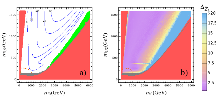
Figure 5: In the $m_{0}\ vs.\ m_{1/2}$ plane of the mSUGRA model for $A_{0}=0$, $\tan\beta=30$ and $\mu>0$, we plot a). contours of $\Omega_{\widetilde{Z}_{1}}h^{2}$ and b). regions of fine-tuning parameter $\Delta_{\widetilde{Z}_{1}}$.

We plot in Fig. 6 the mSUGRA plane for $\tan\beta=53$. In this case, a large new green-shaded region is opening up along the low $m_{0}$ edge of parameter space. This is due to three effects occuring at large $\tan\beta$. 1. The $\tilde{\tau}_{1}$ mass decreases with $\tan\beta$, leading to increased annihilation into $\tau\bar{\tau}$ final states; this increases the area of the bulk annihilation region. 2. The tau and $b$ Yukawa couplings $f_{\tau}$ and $f_{b}$ increase, thus enhancing annihilation into $\tau\bar{\tau}$ and $b\bar{b}$ final states. 3. The value of $m_{A}$ is decreasing while the width $\Gamma_{A}$ is increasing (due to increasing Yukawa couplings that enter the $A$ decay modes), so that $\widetilde{Z}_{1}\widetilde{Z}_{1}\rightarrow A^{(*)}\rightarrow b\bar{b},\ \tau\bar{\tau}$ increases: i.e. we are entering the $A$ resonance annihilation region[30], which enhances the neutralino annihilation cross section in the early universe, thus lowering the relic density. In the case of $\tan\beta=53$, we see that the HB/FP region is still highly fine-tuned. However, broad portions of the low $m_{0}$ mSUGRA parameter space around $m_{1/2}\sim 300-600$ have $\Delta_{\widetilde{Z}_{1}}\stackrel{{\scriptstyle<}}{{\sim}}3$ due to an overlap of bulk annihilation through staus, stau co-annihilation and $A$-resonance annihilation. Another low fine-tuning and relic density consistent region occurs at $m_{1/2}\sim 1200$ GeV, where one sits atop the $A$-resonance.

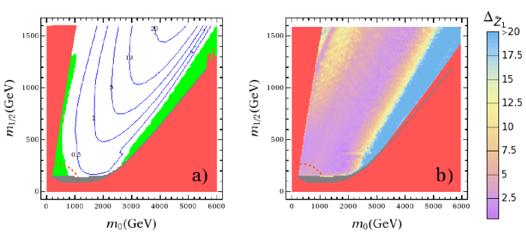
Figure 6: In the $m_{0}\ vs.\ m_{1/2}$ plane of the mSUGRA model for $A_{0}=0$, $\tan\beta=53$ and $\mu>0$, we plot a). contours of $\Omega_{\widetilde{Z}_{1}}h^{2}$ and b). regions of fine-tuning parameter $\Delta_{\widetilde{Z}_{1}}$.

In Fig. 7, we show the mSUGRA plane for $\tan\beta=55$. Here, the $A$-resonance annihilation region is fully displayed, and the $A$ width is even larger. While much of the HB/FP region is still very fine-tuned, the regions of annihilation though the broad $A$ resonance yield relatively low fine-tuning, especially if one sits right on the resonance, or sits in the resonance/bulk/co-annihilation overlap region at low $m_{0}$ and low $m_{1/2}$.

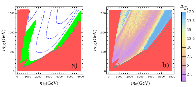
Figure 7: In the $m_{0}\ vs.\ m_{1/2}$ plane of the mSUGRA model for $A_{0}=0$, $\tan\beta=55$ and $\mu>0$, we plot a). contours of $\Omega_{\widetilde{Z}_{1}}h^{2}$ and b). regions of fine-tuning parameter $\Delta_{\widetilde{Z}_{1}}$.

2.3 Results from variation in $A_{0}$ and $\tan\beta$

As mentioned earlier, including $A_{0}$ into the measure of fine-tuning typically yields only a small effect, unless one is near the top-squark co-annihilation region. This is because variation in $A_{0}$ mainly leads to different mixing in the third generation scalar system, and for most of mSUGRA parameter space, affects mainly the top squark mass eigenstates. To show this explicitly, we plot in Fig. 8a). the value of $\Omega_{\widetilde{Z}_{1}}h^{2}$ and in frame b). the value of $|\Delta_{A_{0}}|$ versus variation in $A_{0}$ for two cases: 1. $m_{0}=1.5$ TeV and $m_{1/2}=250$ GeV (blue curves) and 2. $m_{0}=2$ TeV and $m_{1/2}=750$ GeV (red dashed curve), for $\tan\beta=10$ and $\mu>0$. In these two cases, the slope of $\Omega_{\widetilde{Z}_{1}}h^{2}$ is rather mild, leading to a contribution to $|\Delta_{A_{0}}|$ of typically 1 or less. The exception comes for the $m_{1/2}=750$ GeV curve around $A_{0}\sim-4$ TeV, where indeed the value of $m_{\tilde{t}_{1}}$ is rapidly becoming lighter, and feeding into the relic density calculation.

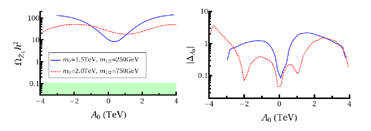
Figure 8: Plot of a). $\Omega_{\widetilde{Z}_{1}}h^{2}$ and b). $|\Delta_{A_{0}}|$ versus $A_{0}$ for two slices out of mSUGRA parameter space: 1. $m_{0}=1.5$ TeV and $m_{1/2}=250$ GeV (blue curves) and 2. $m_{0}=2$ TeV and $m_{1/2}=750$ GeV (red dashed curve), for $\tan\beta=10$ and $\mu>0$.

In Fig. 9, we show a). the relic density and b). $|\Delta_{\tan\beta}|$ versus variation in $\tan\beta$ for 1. $m_{0}=1.5$ TeV and $m_{1/2}=250$ GeV (blue curves) and 2. $m_{0}=2$ TeV and $m_{1/2}=750$ GeV (red dashed curve), for $A_{0}=0$ and $\mu>0$. For most of the $\tan\beta$ values, the relic density varies only slowly with $\tan\beta$, leading to only small contributions to $\Delta$. When $\tan\beta$ becomes of order 50, then $m_{A}$ is rapidly decreasing, and $\Gamma_{A}$ is rapidly increasing, leading to a high rate of neutralino annihilation through the $A^{0}$ resonance. In this case, while fine-tuning with respect to $m_{0}$ and $m_{1/2}$ is low, fine-tuning with respect to $\tan\beta$ is high.

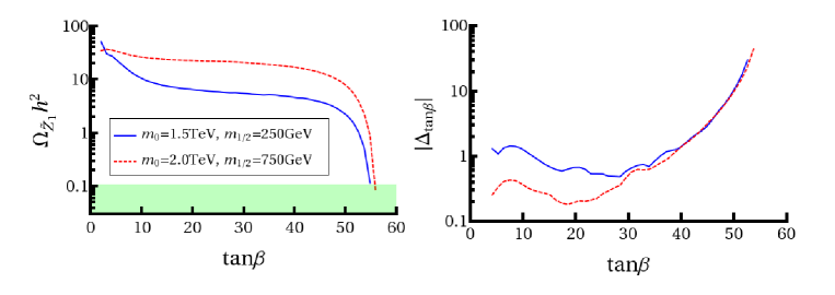
Figure 9: Plot of a). $\Omega_{\widetilde{Z}_{1}}h^{2}$ and b). $|\Delta_{\tan\beta}|$ versus $\tan\beta$ for two slices out of mSUGRA parameter space: 1. $m_{0}=1.5$ TeV and $m_{1/2}=250$ GeV (blue curves) and 2. $m_{0}=2$ TeV and $m_{1/2}=750$ GeV (red dashed curve), for $A_{0}=0$ and $\mu>0$.

In Fig. 10, we show the value of $\Delta$ including contributions from variation in $m_{0}$, $m_{1/2}$ and $\tan\beta$, for the large values of a). $\tan\beta=53$ and b). $\tan\beta=55$. Here, over essentially all of parameter space, the value of $\Delta$ has increased to much larger values than those for $\Delta_{\widetilde{Z}_{1}}$ as shown in Fig’s 6 and 7. Thus, inclusion of $\tan\beta$ in the fine-tuning calculation shows that large values of $\tan\beta\stackrel{{\scriptstyle>}}{{\sim}}50$ result in large fine-tuning of the relic density.

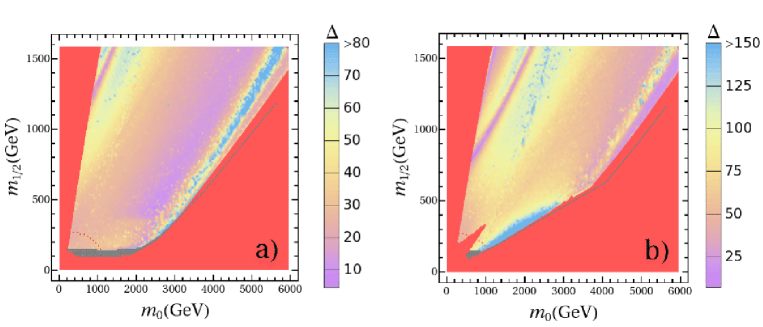
Figure 10: Plot of $\Delta$ in the $m_{0}\ vs.\ m_{1/2}$ plane including variation of $m_{0}$, $m_{1/2}$ and $\tan\beta$ for $A_{0}=0$, $\mu>0$ and a). $\tan\beta=53$ and b). $\tan\beta=55$.

3 The gravitino problem, leptogenesis, and the re-heat temperature

In this section, we review the gravitino problem, baryogenesis via leptogenesis, and production of mixed axion/axino dark matter in the early universe. The reader who is familiar with these issues may proceed directly to Sec. 4; others may wish to follow the brief treatment given here and in Ref. [16].

3.1 The gravitino problem

In supergravity models, supersymmetry is broken via the superHiggs mechanism. The common scenario is to postulate the existence of a hidden sector which is uncoupled to the MSSM sector except via gravity. The superpotential of the hidden sector is chosen such that supergravity is broken, which causes the gravitino (which serves as the gauge particle for the superHiggs mechanism) to develop a mass $m_{3/2}\sim m^{2}/M_{Pl}\sim m_{weak}$. Here, $m$ is a hidden sector parameter assumed to be of order $10^{11}$ GeV. In addition to a mass for the gravitino, SSB masses of order $m_{weak}$ are generated for all scalar, gaugino, trilinear and bilinear SSB terms. Here, we will assume that $m_{3/2}$ is larger than the lightest MSSM mass eigenstate, so that the gravitino essentially decouples from all collider phenomenology.

In all SUGRA scenarios, a potential problem arises for weak-scale gravitinos: the gravitino problem. In this case, gravitinos $\tilde{G}$ can be produced thermally in the early universe (even though the gravitinos are too weakly coupled to be in thermal equilibrium) at a rate which depends on the re-heat temperature $T_{R}$ of the universe. The produced $\tilde{G}$ can then decay to various sparticle-particle combinations, with a long lifetime of order $1-10^{5}$ sec (due to the Planck suppressed gravitino coupling constant). The late gravitino decays occur during or after BBN, and their energy injection into the cosmic soup threatens to destroy the successful BBN predictions of the light element abundances. The precise constraints of BBN on the gravitino mass and $T_{R}$ are presented recently in Ref. [32]. One way to avoid the gravitino problem in the case where $m_{3/2}\stackrel{{\scriptstyle<}}{{\sim}}5$ TeV is to maintain a value of $T_{R}\stackrel{{\scriptstyle<}}{{\sim}}10^{5}$ GeV. Such a low value of $T_{R}$ rules out many attractive baryogenesis mechanisms, and so here instead we assume that $m_{3/2}\stackrel{{\scriptstyle>}}{{\sim}}5$ TeV. In this case, the $\tilde{G}$ is so heavy that its lifetime is of order 1 sec or less, and the $\tilde{G}$ decays near the onset of BBN. In this case, values of $T_{R}$ as large as $10^{9}$ GeV are allowed.

In the simplest SUGRA models, one typically finds $m_{0}=m_{3/2}$. For more general SUGRA models, the scalar masses are in general non-degenerate and only of order $m_{3/2}$[33]. Here for simplicity, we will assume degeneracy of scalar masses, but with $m_{0}\ll m_{3/2}$.

3.1.1 Leptogenesis

One possible baryogenesis mechanism that requires relatively low $T_{R}\sim m_{weak}$ is electroweak baryogenesis. However, calculations of successful electroweak baryogenesis within the MSSM context seem to require sparticle mass spectra with $m_{h}\stackrel{{\scriptstyle<}}{{\sim}}120$ GeV, and $m_{\tilde{t}_{1}}\stackrel{{\scriptstyle<}}{{\sim}}125$ GeV[34]. The latter requirement is difficult (though not impossible) to achieve in the MSSM, and is also partially excluded by collider searches for light top squarks[35]. We will not consider this possibility further.

An alternative attractive mechanism– especially in light of recent evidence for neutrino mass– is thermal leptogenesis[36]. In this scenario, heavy right-handed neutrino states $N_{i}$ ($i=1-3$) decay asymmetrically to leptons versus anti-leptons in the early universe. The lepton-antilepton asymmetry is converted to a baryon-antibaryon asymmetry via sphaleron effects. The measured baryon abundance can be achieved provided the re-heat temperature $T_{R}$ exceeds $\sim 10^{9}$ GeV[37]. The high $T_{R}$ value needed here apparently puts this mechanism into conflict with the gravitino problem in SUGRA theories.

A related leptogenesis mechanism called non-thermal leptogenesis invokes an alternative to thermal production of heavy neutrinos in the early universe. In non-thermal leptogenesis[38], it is possible to have lower re-heat temperatures, since the $N_{i}$ may be generated via inflaton decay. The Boltzmann equations for the $B-L$ asymmetry have been solved numerically in Ref. [39]. The $B-L$ asymmetry is then converted to a baryon asymmetry via sphaleron effects as usual. The baryon-to-entropy ratio is calculated in [39], where it is found

$$\frac{n_{B}}{s}\simeq 8.2\times 10^{-11}\times\left(\frac{T_{R}}{10^{6}\ {\rm GeV}}\right)\left(\frac{2M_{N_{1}}}{m_{\phi}}\right)\left(\frac{m_{\nu_{3}}}{0.05\ {\rm eV}}\right)\delta_{eff},$$ (6)

where $m_{\phi}$ is the inflaton mass and $\delta_{eff}$ is an effective $CP$ violating phase which may be of order 1. Comparing calculation with data (the measured value of $n_{B}/s\simeq 0.9\times 10^{-10}$), a lower bound $T_{R}\stackrel{{\scriptstyle>}}{{\sim}}10^{6}$ GeV may be inferred for viable non-thermal leptogenesis via inflaton decay.

A fourth mechanism for baryogenesis is Affleck-Dine[40] leptogenesis[41]. In this approach, a flat direction $\phi_{i}=(2H\ell_{i})^{1/2}$ is identified in the scalar potential, which may have a large field value in the early universe. When the expansion rate becomes comparable to the SSB terms, the field oscillates, and since the field carries lepton number, coherent oscillations about the potential minimum will develop a lepton number asymmetry. The lepton number asymmetry is then converted to a baryon number asymmetry by sphalerons as usual. Detailed calculations[41] find that the baryon-to-entropy ratio is given by

$$\frac{n_{B}}{s}\simeq\frac{1}{23}\frac{|\langle H\rangle|^{2}T_{R}}{m_{\nu}M_{Pl}^{2}}$$ (7)

where $\langle H\rangle$ is the Higgs field vev, $m_{\nu}$ is the mass of the lightest neutrino and $M_{Pl}$ is the Planck scale. To obtain the observed value of $n_{B}/s$, values of $T_{R}\sim 10^{6}-10^{8}$ are allowed for $m_{\nu}\sim 10^{-9}-10^{-7}$ eV.

Thus, to maintain accord with either non-thermal or Affleck-Dine leptogenesis, along with constraints from the gravitino problem, we will aim for $a\tilde{a}$DM scenarios with $T_{R}\sim 10^{6}-10^{8}$ GeV.

3.2 Mixed axion/axino dark matter

3.2.1 Relic axions

Axions can be produced via various mechanisms in the early universe. Since their lifetime (they decay via $a\rightarrow\gamma\gamma$) turns out to be longer than the age of the universe, they can be a good candidate for dark matter. As we will be concerned here with re-heat temperatures $T_{R}\stackrel{{\scriptstyle<}}{{\sim}}10^{9}\ {\rm GeV}<f_{a}/N$ (to avoid overproducing gravitinos in the early universe), the axion production mechanism relevant for us here is just one: production via vacuum mis-alignment[7]. In this mechanism, the axion field $a(x)$ can have any value $\sim f_{a}$ at temperatures $T\gg\Lambda_{QCD}$. As the temperature of the universe drops, the potential turns on, and the axion field oscillates and settles to its minimum at $-\bar{\theta}f_{a}/N$ (where $\bar{\theta}=\theta+arg(det\ m_{q})$, $\theta$ is the fundamental strong $CP$ violating Lagrangian parameter and $m_{q}$ is the quark mass matrix). The difference in axion field before and after potential turn-on corresponds to the vacuum mis-alignment: it produces an axion number density

$$n_{a}(t)\sim{\frac{1}{2}}m_{a}(t)\langle a^{2}(t)\rangle,$$ (8)

where $t$ is the time near the QCD phase transition. Relating the number density to the entropy density allows one to determine the axion relic density today[7]:

$$\Omega_{a}h^{2}\simeq{\frac{1}{4}}\left(\frac{6\times 10^{-6}\ {\rm eV}}{m_{a}}\right)^{7/6}\theta_{i}^{2}\simeq\frac{1}{4}\left(\frac{f_{a}/N}{10^{12}\ \mathrm{GeV}}\right)^{7/6}\theta_{i}^{2},$$ (9)

where $\theta_{i}$ is the initial vacuum mis-alignment angle, with $-\pi\stackrel{{\scriptstyle<}}{{\sim}}\theta_{i}\stackrel{{\scriptstyle<}}{{\sim}}\pi$. An error estimate of the axion relic density from vacuum mis-alignment is plus-or-minus a factor of three. Axions produced via vacuum mis-alignment would constititute cold dark matter. However, in the event that $\langle a^{2}(t)\rangle$ is inadvertently small, then much lower values of axion relic density could be allowed. Additional entropy production at $t>t_{QCD}$ can also lower the axion relic abundance. Taking the value of Eq. (9) literally, along with $\theta_{i}\simeq 1$, and comparing to the WMAP5 measured abundance of CDM in the universe, one gets an upper bound $f_{a}/N\stackrel{{\scriptstyle<}}{{\sim}}5\times 10^{11}$ GeV, or a lower bound $m_{a}\stackrel{{\scriptstyle>}}{{\sim}}10^{-5}$ eV. If we take the axion relic density a factor of three lower, then the bounds change to $f_{a}/N\stackrel{{\scriptstyle<}}{{\sim}}1.2\times 10^{12}$ GeV, and $m_{a}\stackrel{{\scriptstyle>}}{{\sim}}4\times 10^{-6}$ eV.

3.2.2 Axinos from neutralino decay

If the $\tilde{a}$ is the lightest SUSY particle, then the $\widetilde{Z}_{1}$ will no longer be stable, and can decay via $\widetilde{Z}_{1}\rightarrow\tilde{a}\gamma$. The relic abundance of axinos from neutralino decay (non-thermal production, or $NTP$) is given simply by

$$\Omega_{\tilde{a}}^{NTP}h^{2}=\frac{m_{\tilde{a}}}{m_{\widetilde{Z}_{1}}}\Omega_{\widetilde{Z}_{1}}h^{2},$$ (10)

since in this case the axinos inherit the thermally produced neutralino number density. The neutralino-to-axino decay offers a mechanism to shed large factors of relic density. For a case where $m_{\widetilde{Z}_{1}}\sim 100$ GeV and $\Omega_{\widetilde{Z}_{1}}h^{2}\sim 10$ (as can occur in the mSUGRA model at large $m_{0}$ values) an axino mass of less than 1 GeV reduces the DM abundance to below WMAP-measured levels.

The lifetime for these decays has been calculated, and it is typically in the range of $\tau(\widetilde{Z}_{1}\rightarrow\tilde{a}\gamma)\sim 0.01-1$ sec[13]. The photon energy injection from $\widetilde{Z}_{1}\rightarrow\tilde{a}\gamma$ decay into the cosmic soup occurs typically before BBN, thus avoiding the constraints that plague the case of a gravitino LSP[32]. The axino DM arising from neutralino decay is generally considered warm or even hot dark matter for cases with $m_{\tilde{a}}\stackrel{{\scriptstyle<}}{{\sim}}1-10$ GeV[42]. Thus, in the mSUGRA scenario considered here, where $m_{\tilde{a}}\stackrel{{\scriptstyle<}}{{\sim}}1-10$ GeV, we usually get warm axino DM from neutralino decay.

3.2.3 Thermal production of axinos

Even though axinos may not be in thermal equilibrium in the early universe, they can still be produced thermally via scattering and decay processes in the cosmic soup. The axino thermally produced (TP) relic abundance has been calculated in Ref. [13, 43], and is given in Ref. [43] using hard thermal loop resummation as

$$\Omega_{\tilde{a}}^{TP}h^{2}\simeq 5.5g_{s}^{6}\ln\left(\frac{1.211}{g_{s}}\right)\left(\frac{10^{11}\ {\rm GeV}}{f_{a}/N}\right)^{2}\left(\frac{m_{\tilde{a}}}{0.1\ {\rm GeV}}\right)\left(\frac{T_{R}}{10^{4}\ {\rm GeV}}\right)$$ (11)

where $g_{s}$ is the strong coupling evaluated at $Q=T_{R}$ and $N$ is the model dependent color anomaly of the PQ symmetry, of order 1. For reference, we take $g_{s}(T_{R}=10^{6}\ {\rm GeV})=0.932$ (as given by Isajet 2-loop $g_{s}$ evolution in mSUGRA), with $g_{s}$ at other values of $T_{R}$ given by the 1-loop MSSM running value. The thermally produced axinos qualify as cold dark matter as long as $m_{\tilde{a}}\stackrel{{\scriptstyle>}}{{\sim}}0.1$ MeV[13, 43].

4 Fine-tuning in mSUGRA with mixed axion/axino CDM

In this section, we calculate the fine-tuning parameter for the dark matter relic density in models with mixed $a\tilde{a}$DM: $\Delta_{a\tilde{a}}$. Contributions to $\Delta_{a\tilde{a}}$ are calculated from both the axion relic density and the thermally produced axino relic density. We do not include the non-thermally produced axino relic density as it makes a tiny contribution to the total for the values of $m_{\tilde{a}}\sim 1$ MeV considered here (see Figs. 2 and 3 of Ref. [16]). We take the total relic density to be

$$\Omega_{a\tilde{a}}h^{2} =\Omega_{a}h^{2}+\Omega^{TP}_{\tilde{a}}h^{2}$$ (12)

$$=\frac{1}{4}\left(\frac{f_{a}/N}{10^{12}\ \mathrm{GeV}}\right)^{7/6}\theta_{i}^{2}+5.5g^{6}_{s}\ln{\left(\frac{1.211}{g_{s}}\right)}\left(\frac{10^{11}\ \mathrm{GeV}}{f_{a}/N}\right)^{2}\left(\frac{m_{\tilde{a}}}{0.1\ \mathrm{GeV}}\right)\left(\frac{T_{R}}{10^{4}\ \mathrm{GeV}}\right)$$ (13)

and calculate the total $\Delta_{a\tilde{a}}$ exactly by differentiating (13) with respect to $f_{a}/N$, $T_{R}$ and $m_{\tilde{a}}$. We find:

$$\Delta_{T_{R}} =\frac{T_{R}}{\Omega_{a\tilde{a}}h^{2}}\frac{\partial\Omega_{a\tilde{a}}h^{2}}{\partial T_{R}}=\frac{T_{R}}{\Omega_{a\tilde{a}}h^{2}}5.5g^{6}_{s}\ln{\left(\frac{1.211}{g_{s}}\right)}\left(\frac{10^{11}\ \mathrm{GeV}}{f_{a}/N}\right)^{2}\left(\frac{m_{\tilde{a}}}{0.1\ \mathrm{GeV}}\right)\left(\frac{1}{10^{4}\ \mathrm{GeV}}\right)$$ (14)

$$\Delta_{m_{\tilde{a}}} =\frac{m_{\tilde{a}}}{\Omega_{a\tilde{a}}h^{2}}\frac{\partial\Omega_{a\tilde{a}}h^{2}}{\partial m_{\tilde{a}}}=\frac{m_{\tilde{a}}}{\Omega_{a\tilde{a}}h^{2}}5.5g^{6}_{s}\ln{\left(\frac{1.211}{g_{s}}\right)}\left(\frac{10^{11}\ \mathrm{GeV}}{f_{a}/N}\right)^{2}\left(\frac{1}{0.1\ \mathrm{GeV}}\right)\left(\frac{T_{R}}{10^{4}\ \mathrm{GeV}}\right)$$ (15)

and

$$\Delta_{f_{a}/N} =\frac{f_{a}/N}{\Omega_{a\tilde{a}}h^{2}}\frac{\partial\Omega_{a\tilde{a}}h^{2}}{\partial f_{a}/N}$$ (16)

$$\begin{split}&=\frac{f_{a}/N}{\Omega_{a\tilde{a}}h^{2}}\left[\frac{7}{24}\left(\frac{1}{10^{12}\ \mathrm{GeV}}\right)^{7/6}\left(f_{a}/N\right)^{1/6}\theta_{i}^{2}\right.\\ &\qquad\qquad-\left.11g^{6}_{s}\ln{\left(\frac{1.211}{g_{s}}\right)}\left(10^{11}\ \mathrm{GeV}\right)^{2}\left(\frac{1}{f_{a}/N}\right)^{3}\left(\frac{m_{\tilde{a}}}{0.1\ \mathrm{GeV}}\right)\left(\frac{T_{R}}{10^{4}\ \mathrm{GeV}}\right)\right],\end{split}$$ (17)

and

$$\Delta_{\theta_{i}}=\frac{\theta_{i}}{\Omega_{a\tilde{a}}h^{2}}\frac{\partial\Omega_{a\tilde{a}}h^{2}}{\partial\theta_{i}}=2\frac{\Omega_{a}h^{2}}{\Omega_{a\tilde{a}}h^{2}}.$$ (18)

The total fine tuning parameter is then given by

$$\Delta_{a\tilde{a}}=\sqrt{\Delta_{T_{R}}^{2}+\Delta_{m_{\tilde{a}}}^{2}+\Delta_{f_{a}/N}^{2}+\Delta_{\theta_{i}}^{2}}.$$ (19)

We plot our first results in the $f_{a}/N\ vs.\ T_{R}$ plane, keeping $m_{\tilde{a}}$ fixed at 1 MeV: see Fig. 11. In frame a)., we show contours of $\Omega_{a\tilde{a}}h^{2}$. The green region gives $\Omega_{a\tilde{a}}<0.11$, and so is consistent with WMAP. In frame b)., we show regions of fine-tuning $\Delta_{a\tilde{a}}$. The scale is shown on the right edge of the plot. Note in this case the entire plane has $\Delta_{a\tilde{a}}<2.5$, so there is very little fine-tuning across the entire plane of parameter space. The left region, color-coded dark blue, is the region of dominantly thermally produced axino CDM, whilst the right-most region, color-coded lighter blue, is dominantly axion CDM. In this region, the fine-tuning parameter $\Delta_{a\tilde{a}}\simeq 2.3$. The intermediate region, shaded by yellow and purple bands, is the region of mixed $a\tilde{a}$CDM: the purple band has very low fine-tuning, with $\Delta_{a\tilde{a}}<1.4$. The contour where mixed $a\tilde{a}$CDM saturate the WMAP measured value is shown by the green dashed line. The region where the highest values of $T_{R}$ are found coincide with the region of lowest fine-tuning, with a nearly equal mix of axion and axino CDM.

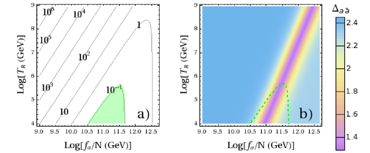
Figure 11: Plot of a). contours of axion/axino relic density $\Omega_{a\tilde{a}}h^{2}$ in the $f_{a}/N\ vs.\ T_{R}$ plane and b). regions of fine-tuning $\Delta_{a\tilde{a}}$ for fixed axino mass $m_{\tilde{a}}=1$ MeV. The green region in a). has $\Omega_{a\tilde{a}}h^{2}\leq 0.11$. The green dashed line in frame b). is where $\Omega_{a\tilde{a}}h^{2}=0.11$.

To gain additional perspective, in Fig. 12 we show the mixed axion/axino relic density as a 3-d plot in the $f_{a}/N\ vs.\ T_{R}$ plane for $m_{\tilde{a}}=1$ MeV. The level of fine-tuning, corresponding to the slope of the surface, is rather low throughout, since there are no regions with a steep slope. The fine-tuning is minimal along the trough running through the right-center of the plot.

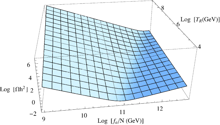
Figure 12: A 3-d plot of axion/axino relic density in the $f_{a}/N\ vs.\ T_{R}$ plane of the $a\tilde{a}$ augmented mSUGRA model.

To better understand the situation with mixed $a\tilde{a}$CDM, we show in Fig. 13 a slice of our Fig. 11 with constant $T_{R}=10^{5}$ GeV. In frame a)., we see that the value of $\Omega_{a\tilde{a}}h^{2}$ initially drops as $f_{a}/N$ increases. This is in the region of dominant axino CDM, and increasing $f_{a}/N$ decreases the axino coupling strength, and hence suppresses its thermal production in the early universe. As $f_{a}/N$ increases further, the relic abundance of axions steadily increases, until around $f_{a}/N\sim 2\times 10^{11}$ GeV there is an upswing in the relic abundance. This is the stable fine-tuning region since small fluctuations of parameters about this point do not substantially alter the axino/axino relic density. The fine-tuning parameter $\Delta_{a\tilde{a}}$ is shown in frame b).. Here, we see that the fine-tuning is slightly high in the region of mainly axino CDM, with low $f_{a}/N$, but reaches a minimum at the point of equal admixture. The value of $\Delta_{a\tilde{a}}$ doesn’t extend all the way to zero, in spite of the zero slope shown, because $\Delta_{a\tilde{a}}$ still varies with $m_{\tilde{a}}$, $T_{R}$ and $\theta_{i}$. The fine-tuning parameter increases to the analytic value of $2.3$ as $f_{a}/N$ increases further, into the region of mainly axion CDM.

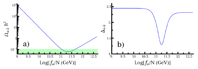
Figure 13: Plot of a). axion/axino relic density $\Omega_{a\tilde{a}}h^{2}$ and b). fine-tuning parameter $\Delta_{a\tilde{a}}$ versus $f_{a}/N$ for fixed axino mass $m_{\tilde{a}}=1$ MeV and fixed re-heat temperature $T_{R}=10^{5}$ GeV.

A similar plot to Fig. 11 is shown in Fig. 14, but in this case taking $m_{\tilde{a}}=0.1$ MeV. Note that this value yields the approximate dividing line given in Refs. [13, 43] below which the thermally produced axinos would be mainly warm DM instead of cold DM. In any case, in frame a)., we see that the WMAP allowed region has expanded, and now values of $T_{R}$ as high as $5\times 10^{6}$ GeV are allowed, making the scenario consistent with at least non-thermal leptogenesis. The region of maximal $T_{R}$ also coincides with the region of least fine-tuning, with a roughly equal admixture of axion and thermally produced axino DM.

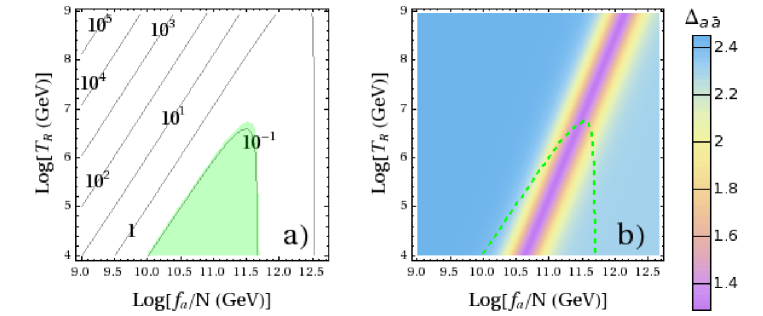
Figure 14: Plot of a). contours of axion/axino relic density $\Omega_{a\tilde{a}}h^{2}$ in the $f_{a}/N\ vs.\ T_{R}$ plane and b). regions of fine-tuning $\Delta_{a\tilde{a}}$ for fixed axino mass $m_{\tilde{a}}=0.1$ MeV. The green region in a). has $\Omega_{a\tilde{a}}h^{2}\leq 0.11$. The green dashed line in frame b). is where $\Omega_{a\tilde{a}}h^{2}=0.11$.

In Fig. 15 we show the contours of relic density $\Omega_{a\tilde{a}}h^{2}$ in the $m_{\tilde{a}}\ vs.\ T_{R}$ plane for fixed value of $f_{a}/N=4.88\times 10^{11}$ GeV. The large value of $f_{a}/N$ yields a scenario with mainly axion CDM when the WMAP measured abundance is saturated. The green shaded region in frame a). is WMAP-allowed. The red dashed line shows the approximate dividing line between warm and cold thermally produced axinos. In this case, the demarcation line is largely irrelevant, since if $\Omega_{a\tilde{a}}h^{2}\simeq 0.11$, almost all the DM is composed of cold axions, and a tiny admixture of warm axinos would be allowed. In frame b)., we show the regions of fine-tuning $\Delta_{a\tilde{a}}$. Since the WMAP-allowed region coincides with mainly axion CDM, the fine-tuning along the green dashed line is always low: $\Delta_{a\tilde{a}}\sim 2.3$. Note that in the scenario with mainly axion CDM, the value of $T_{R}$ can easily reach to well over $10^{7}$ GeV, allowing for non-thermal or Affleck-Dine leptogenesis.

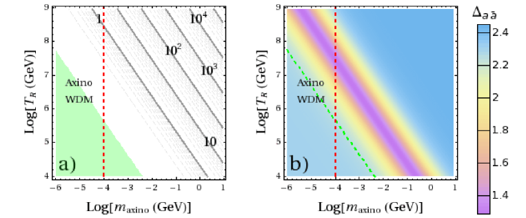
Figure 15: Plot of a). contours of axion/axino relic density $\Omega_{a\tilde{a}}h^{2}$ in the $m_{\tilde{a}}\ vs.\ T_{R}$ plane and b). regions of fine-tuning $\Delta_{a\tilde{a}}$ for fixed $f_{a}/N=4.88\times 10^{11}$ GeV (which gives mainly axion CDM along the line of $\Omega_{a\tilde{a}}=0.11$). The green region in a). has $\Omega_{a\tilde{a}}h^{2}\leq 0.11$. The green dashed line in frame b). is where $\Omega_{a\tilde{a}}h^{2}=0.11$. The region to the left of red-dashed line gives thermally produced warm axino dark matter.

In Fig. 16 we show the $m_{\tilde{a}}\ vs.\ T_{R}$ plane for $f_{a}/N=3\times 10^{11}$ GeV, which gives roughly an equal admixture of axion and thermally produced axino DM. In this case, the value of $T_{R}$ reaches beyond $10^{8}$ GeV, although for very low values of $m_{\tilde{a}}$ where it is expected that the axino will be warm DM. For this scenario, it is unclear how much mixture of warm and cold dark matter is cosmologically allowed. To answer the question, the velocity profile of the warm axinos would have to be fed into $n-body$ simulations of large scale structure formation, to see how well such a mixed warm/cold DM scenario fits the data. At present, we are unaware of such studies. In frame b)., we see that the line of WMAP-saturated abundance lies nearly on top of the region of lowest fine-tuning, with $\Delta_{a\tilde{a}}<1.4$.

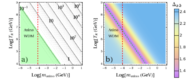
Figure 16: Plot of a). contours of axion/axino relic density $\Omega_{a\tilde{a}}h^{2}$ in the $m_{\tilde{a}}\ vs.\ T_{R}$ plane and b). regions of fine-tuning $\Delta_{a\tilde{a}}$ for fixed $f_{a}/N=3\times 10^{11}$ GeV (which gives a 50-50 mix of axion/axino DM along the line of $\Omega_{a\tilde{a}}=0.11$). The green region in a). has $\Omega_{a\tilde{a}}h^{2}\leq 0.11$. The green dashed line in frame b). is where $\Omega_{a\tilde{a}}h^{2}=0.11$. The region to the left of red-dashed line gives thermally produced warm axino dark matter.

In Fig. 17, we show again the $m_{\tilde{a}}\ vs.\ T_{R}$ plane, but this time for $f_{a}/N=1\times 10^{11}$ GeV, which gives mainly thermally produced axino DM. In this case the region to the left of the red-dashed line should likely be disallowed, since the dominant form of DM will be warm, rather than cold. The region to the right of the $m_{\tilde{a}}=0.1$ MeV line, in the WMAP-allowed region, only allows for $T_{R}$ to reach a max of $10^{6}$ GeV. Furthermore, from frame b)., we see that the fine-tuning parameter in this case for the WMAP-saturated region along the green dashed line is somewhat higher, reaching $\Delta_{a\tilde{a}}\sim 2$.

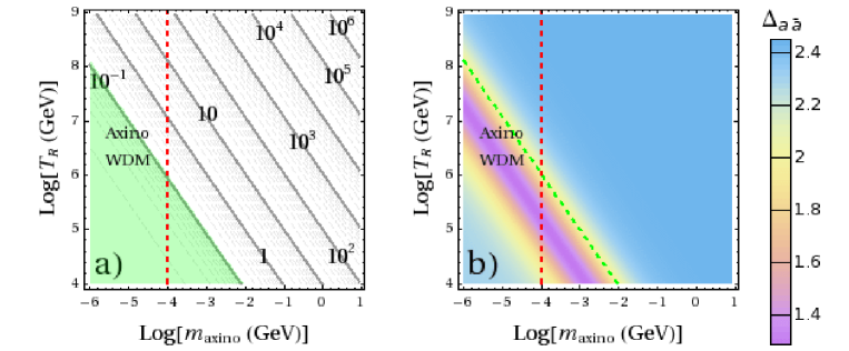
Figure 17: Plot of a). contours of axion/axino relic density $\Omega_{a\tilde{a}}h^{2}$ in the $m_{\tilde{a}}\ vs.\ T_{R}$ plane and b). regions of fine-tuning $\Delta_{a\tilde{a}}$ for fixed $f_{a}/N=1\times 10^{11}$ GeV (which gives mainly axino DM along the line of $\Omega_{a\tilde{a}}=0.11$). The green region in a). has $\Omega_{a\tilde{a}}h^{2}\leq 0.11$. The green dashed line in frame b). is where $\Omega_{a\tilde{a}}h^{2}=0.11$. The region to the left of red-dashed line gives thermally produced warm axino dark matter.

5 Summary and conclusions

In this paper, we have examined the fine-tuning associated with the relic density of dark matter in the minimal supergravity model. We have calculated a measure of fine-tuning assuming two scenarios for SUSY dark matter: 1. neutralino dark matter with fine-tuning parameter $\Delta_{\widetilde{Z}_{1}}$, and 2. mixed axion/axino dark matter with fine-tuning parameter $\Delta_{a\tilde{a}}$.

In the case of neutralino dark matter, we find that the WMAP-allowed regions of mSUGRA such as the stau co-annihilation region, the HB/FP region and the light Higgs $h$-resonance annihilation region, are all rather highly fine-tuned, especially the HB/FP region, where $\Delta_{\widetilde{Z}_{1}}$ ranges from 20-100. Only mild fine-tuning is found in the low $m_{0}$, low $m_{1/2}$ region where stau co-annihilation and bulk annihilation through $t$-channel slepton exchange overlap. If one moves to large $\tan\beta\sim 50$, then larger regions of parameter space which are consistent with WMAP occur. These large $\tan\beta$ regions have modest fine-tuning versus $m_{0}$ and $m_{1/2}$, but very large fine-tuning versus $\tan\beta$.

If instead we assume that dark matter is composed of an axion/axino admixture, rather than neutralinos, then we find that the relic density fine-tuning parameter is generically much lower: $\Delta_{a\tilde{a}}\sim 1.3-2.5$ throughout parameter space. Here, we have assumed the existence of a light axino with mass $m_{\tilde{a}}\sim$ keV-MeV. Such a light axino opens up all of mSUGRA parameter space to being WMAP allowed, since now the neutralino decays via $\widetilde{Z}_{1}\rightarrow\tilde{a}\gamma$. If the DM is dominated by thermally produced axinos, then the re-heat temperature $T_{R}$ is generally lower than $10^{6}$ GeV unless the axinos are actually warm dark matter ($m_{\tilde{a}}\stackrel{{\scriptstyle<}}{{\sim}}100$ keV), so this scenario seems rather unlikely. However, if the PQ breaking scale $f_{a}/N$ is large, then the DM can be either a nearly equal axion/axino admixture, in which case fine-tuning is lowest ($\Delta_{a\tilde{a}}\sim 1.3$), or a dominantly axion mixture (in which case $\Delta_{a\tilde{a}}\sim 2.3$). Either scenario easily admits $T_{R}>10^{6}$ GeV, which can allow for non-thermal leptogenesis to occur.

The consequences of the mixed $a\tilde{a}$CDM scenario for future dark matter searches is as follows. For collider searches, we expect much the same collider signatures as in the mSUGRA model with neutralino dark matter, since we assume the $\widetilde{Z}_{1}$ is the NLSP, and decays far outside the collider detectors. However, all of mSUGRA parameter space is now WMAP-allowed, instead of just the special co-annihilation, HB/FP region and resonance annihilation regions. As shown in Ref. [16], the regions of WMAP-allowed neutralino CDM yield the lowest values of $T_{R}$, and so the stau co-annihilation, HB/FP region and $h$ resonance annihilation regions are most dis-favored for the case of mixed $a\tilde{a}$CDM.

As far as WIMP searches go, in the mixed $a\tilde{a}$CDM scenario, we expect no positive signals if $m_{\widetilde{Z}_{1}}>m_{\tilde{a}}$. If $m_{\tilde{a}}>m_{\widetilde{Z}_{1}}$, then the $\widetilde{Z}_{1}$ would still be stable (assuming $R$-parity conservation) and WIMP direct and indirect detection signals are still possible[45]. In the case of large axion relic abundance, which appears to us to be the favored scenario, then a positive signal at relic axion search experiments such as ADMX might be expected[46], although solar axion searches are less likely to achieve positive results, since large values of $f_{a}/N$ are favored, leading to small axion/axino couplings.

Our analysis has been based on the admittedly subjective basis of fine-tuning of the relic density of dark matter relative to model input parameters. We note here that the mSUGRA model already needs substantial fine-tuning in the electroweak sector in order to accomodate the relatively light $Z$ boson mass in the face of limits on the soft SUSY breaking parameters[47] (the little hierarchy problem). Our philosophy here is that less fine-tuning is better, and high fine-tuning in one sector is better than high fine-tuning in two sectors, e.g. electroweak and dark matter sectors.

While our analysis has been restricted to the mSUGRA SUSY model, one might ask how general our conclusions might be. In SUSY models based on gravity mediation, with a neutralino LSP, the DM relic density is generically too high unless some special mechanism is acting to enhance the neutralino annihilation cross section in the early universe. For instance, in SUSY models with non-universality, instead of stau or stop co-annihilation, one might have sbottom or sneutrino co-annihilation, or bino-wino co-annihilation: in any case, the mass gap between co-annihilating particles must be fine-tuned to obtain agreement with the measured dark matter abundance. In non-universal models with a well-tempered neutralino[48], where the neutralino bino-higgsino or bino-wino composition is adjusted to fit the measured relic density, other parameters (Higgs soft masses, gaugino masses) must be fine-tuned to get just the right “tempering”, as occurs in the mSUGRA HB/FP region. In other models, Higgs soft mass terms can be adjusted to allow $2m_{\widetilde{Z}_{1}}$ to sit atop the $A$ resonance; but again, in this case, parameters must be fine-tuned (unless $\tan\beta$ is large, which also occurs in mSUGRA). The case where the SUSY neutralino abundance is not fine-tuned has long been noted: it is where squarks and sleptons are so light that $t$-channel annihilation channels are large. However, LEP2 search limits now essentially exclude all these regions. Thus, although we restrict our analysis here to the mSUGRA model, we feel this model provides a sort of microcosm for general SUSY models, in that it illustrates many of the features common to all SUSY models.

Our main conclusion is this. In the world HEP community, a tremendous effort is underway to explore for WIMP cold dark matter, based partly on the view that SUSY models naturally give rise to the “WIMP-miracle”, and an excellent WIMP candidate for CDM. We have shown here that at least for the paradigm SUSY model– mSUGRA– usually a large overabundance of neutralino CDM is produced, unless one lies along a region of very high fine-tuning, where a slight change in model parameters leads to a large change in relic density: this equates to a high degree of relic density fine-tuning. Alternatively, if one assumes the PQWW solution to the strong CP problem within SUSY models, and a very light axino with $m_{\tilde{a}}$ of the order of MeV, then along with an elegant solution to the strong CP problem, one obtains a mixed axion/axino relic density with much less fine-tuning. Given our results, we would advocate that a much increased share of HEP resources be given to relic axion searches, where the global search effort has been much more limited.

- [1] J. Dunkley et al. [WMAP Collaboration], Astrophys. J. Suppl. 180 (2009) 306
- [2] For a recent review, see P. Sikivie, hep-ph/0509198; M. Turner, Phys. Rept. 197 (1990) 67; J. E. Kim and G. Carosi, arXiv:0807.3125 (2008).
- [3] R. Peccei and H. Quinn, Phys. Rev. Lett. 38 (1977) 1440 and Phys. Rev. D 16 (1977) 1791.
- [4] S. Weinberg, Phys. Rev. Lett. 40 (1978) 223; F. Wilczek, Phys. Rev. Lett. 40 (1978) 279.
- [5] J. E. Kim, Phys. Rev. Lett. 43 (1979) 103; M. A. Shifman, A. Vainstein and V. I. Zakharov, Nucl. Phys. B 166 (1980) 493.
- [6] M. Dine, W. Fischler and M. Srednicki, Phys. Lett. B 104 (1981) 199; A. P. Zhitnitskii, Sov. J. Nucl. 31 (1980) 260.
- [7] L. F. Abbott and P. Sikivie, Phys. Lett. B 120 (1983) 133; J. Preskill, M. Wise and F. Wilczek, Phys. Lett. B 120 (1983) 127; M. Dine and W. Fischler, Phys. Lett. B 120 (1983) 137; M. Turner, Phys. Rev. D 33 (1986) 889; K. J. Bae, J. H. Huh and J. E. Kim, JCAP0809 (2008) 005; L. Visinelli and P. Gondolo, Phys. Rev. D 80 (2009) 035024.
- [8] H. P. Nilles and S. Raby, Nucl. Phys. B 198 (1982) 102.
- [9] For recent reviews of axion/axino dark matter, see F. Steffen, Eur. Phys. J. C 59 (2009) 557; L. Covi and J. E. Kim, New J. Phys. 11 (2009) 105003.
- [10] T. Goto and M. Yamaguchi, Phys. Lett. B 276 (1992) 103; E. J. Chun, J. E. Kim and H. P. Nilles, Phys. Lett. B 287 (1992) 123.
- [11] K. Rajagopal, M. Turner and F. Wilczek, Nucl. Phys. B 358 (1991) 447.
- [12] E. J. Chun and A. Lukas, Phys. Lett. B 357 (1995) 43.
- [13] L. Covi, J. E. Kim and L. Roszkowski, Phys. Rev. Lett. 82 (1999) 4180; L. Covi, H. B. Kim, J. E. Kim and L. Roszkowski, J. High Energy Phys. 0105 (2001) 033. L. Covi, L. Roszkowski and Small, J. High Energy Phys. 0207 (2002) 023.
- [14] A. Freitas, F. Steffen, N. Tajuddin and D. Wyler, Phys. Lett. B 679 (2009) 270.
- [15] L. Covi, L. Roszkowski, R. Ruiz de Austri and M. Small, J. High Energy Phys. 0406 (2004) 003; A. Brandenburg, L. Covi, K. Hamaguchi, L. Roszkowski and F. Steffen, Phys. Lett. B 617 (2005) 99; K. Y. Choi, L. Roszkowski and R. Ruiz de Austri, J. High Energy Phys. 0804 (2008) 016.
- [16] H. Baer, A. Box and H. Summy, J. High Energy Phys. 0908 (2009) 080.
- [17] A. Chamseddine, R. Arnowitt and P. Nath, Phys. Rev. Lett. 49 (1982) 970; R. Barbieri, S. Ferrara and C. Savoy, Phys. Lett. B 119 (1982) 343; N. Ohta, Prog. Theor. Phys. 70 (1983) 542; L. Hall, J. Lykken and S. Weinberg, Phys. Rev. D 27 (1983) 2359.
- [18] P. Sikivie and Q. Yang, Phys. Rev. Lett. 103 (2009) 111301.
- [19] H. Baer, S. Kraml, S. Sekmen and H. Summy, J. High Energy Phys. 0803 (2008) 056 ; H. Baer and H. Summy, Phys. Lett. B 666 (2008) 5; H. Baer, M. Haider, S. Kraml, S. Sekmen and H. Summy, JCAP0902 (2009) 002.
- [20] J. Ellis and K. Olive, Phys. Lett. B 514 (2001) 114.
- [21] F. Paige, S. Protopopescu, H. Baer and X. Tata, hep-ph/0312045; http://www.nhn.ou.edu/isajet/
- [22] H. E. Haber, R. Hempfling and A. Hoang, Z. Physik C 75 (1996) 539.
- [23] D.Pierce, J. Bagger, K. Matchev and R. Zhang, Nucl. Phys. B 491 (1997) 3.
- [24] H. Baer, C. Balazs, A. Belyaev, J. High Energy Phys. 0203 (2002) 042.
- [25] H. Baer, C. H. Chen, M. Drees, F. Paige and X. Tata, Phys. Rev. Lett. 79 (1997) 986.
- [26] K. L. Chan, U. Chattopadhyay and P. Nath, Phys. Rev. D 58 (1998) 096004 ; J. Feng, K. Matchev and T. Moroi, Phys. Rev. Lett. 84 (2000) 2322 and Phys. Rev. D 61 (2000) 075005; see also H. Baer, C. H. Chen, F. Paige and X. Tata, Phys. Rev. D 52 (1995) 2746 and Phys. Rev. D 53 (1996) 6241; H. Baer, C. H. Chen, M. Drees, F. Paige and X. Tata, Phys. Rev. D 59 (1999) 055014; for a model-independent approach, see H. Baer, T. Krupovnickas, S. Profumo and P. Ullio, J. High Energy Phys. 0510 (2005) 020.
- [27] J. Ellis, T. Falk and K. Olive, Phys. Lett. B 444 (1998) 367; J. Ellis, T. Falk, K. Olive and M. Srednicki, Astropart. Phys. 13 (2000) 181; M.E. Gómez, G. Lazarides and C. Pallis, Phys. Rev. D 61 (2000) 123512 and Phys. Lett. B 487 (2000) 313; A. Lahanas, D. V. Nanopoulos and V. Spanos, Phys. Rev. D 62 (2000) 023515; R. Arnowitt, B. Dutta and Y. Santoso, Nucl. Phys. B 606 (2001) 59; see also Ref. [24].
- [28] R. Arnowitt and P. Nath, Phys. Rev. Lett. 70 (1993) 3696; H. Baer and M. Brhlik, Phys. Rev. D 53 (1996) 597; A. Djouadi, M. Drees and J. Kneur, Phys. Lett. B 624 (2005) 60.
- [29] H. Goldberg, Phys. Rev. Lett. 50 (1983) 1419; J. Ellis et al. Nucl. Phys. B 238 (1984) 453; P. Nath and R. Arnowitt, Phys. Rev. Lett. 70 (1993) 3696; H. Baer and M. Brhlik, Ref. [28]; V. Barger and C. Kao, Phys. Rev. D 57 (1998) 3131.
- [30] M. Drees and M. Nojiri, Phys. Rev. D 47 (1993) 376; H. Baer and M. Brhlik, Phys. Rev. D 57 (1998) 567; H. Baer, M. Brhlik, M. Diaz, J. Ferrandis, P. Mercadante, P. Quintana and X. Tata, Phys. Rev. D 63 (2001) 015007; J. Ellis, T. Falk, G. Ganis, K. Olive and M. Srednicki, Phys. Lett. B 510 (2001) 236; L. Roszkowski, R. Ruiz de Austri and T. Nihei, J. High Energy Phys. 0108 (2001) 024; A. Djouadi, M. Drees and J. L. Kneur, J. High Energy Phys. 0108 (2001) 055; A. Lahanas and V. Spanos, Eur. Phys. J. C 23 (2002) 185.
- [31] J. E. Kim and H. P. Nilles, Phys. Lett. B 138 (1984) 150.
- [32] K. Kohri, T. Moroi and A. Yotsuyanagi, Phys. Rev. D 73 (2006) 123511; for an update, see M. Kawasaki, K. Kohri, T. Moroi and A. Yotsuyanagi, Phys. Rev. D 78 (2008) 065011; see also J. Pradler and F. D. Steffen, Phys. Lett. B 648 (2007) 224.
- [33] S. Soni and H. A. Weldon, Phys. Lett. B 126 (1983) 215; V.Kaplunovsky and J. Louis, Phys. Lett. B 306 (1993) 269; A. Brignole, L. Ibanez and C. Munoz, Nucl. Phys. B 422 (1994) 125.
- [34] For a recent analysis, see M. Carena, G. Nardini, M. Quiros and C. Wagner, Nucl. Phys. B 812 (2009) 243.
- [35] A. A. Affolder et al. [CDF Collaboration], Phys. Rev. Lett. 84 (2000) 5273;
- [36] M. Fukugita and T. Yanagida, Phys. Lett. B 174 (1986) 45; M. Luty, Phys. Rev. D 45 (1992) 455; W. Buchmüller and M. Plumacher, Phys. Lett. B 389 (1996) 73 and Int. J. Mod. Phys. A 15 (2000) 5047; R. Barbieri, P. Creminelli, A. Strumia and N. Tetradis, Nucl. Phys. B 575 (2000) 61; G. F. Giudice, A. Notari, M. Raidal, A. Riotto and A. Strumia, Nucl. Phys. B 685 (2004) 89; for a recent review, see W. Buchmüller, R. Peccei and T. Yanagida, Ann. Rev. Nucl. Part. Sci. 55 (2005) 311.
- [37] W. Buchmuller, P. Di Bari and M. Plumacher, Annal. Phys. 315 (2005) 305.
- [38] G. Lazarides and Q. Shafi, Phys. Lett. B 258 (1991) 305; K. Kumekawa, T. Moroi and T. Yanagida, Prog. Theor. Phys. 92 (1994) 437; T. Asaka, K. Hamaguchi, M. Kawasaki and T. Yanagida, Phys. Lett. B 464 (1999) 12.
- [39] M. Ibe, T. Moroi and T. Yanagida, Phys. Lett. B 620 (2005) 9.
- [40] I. Affleck and M. Dine, Nucl. Phys. B 249 (1985) 361.
- [41] H. Murayama and T. Yanagida, Phys. Lett. B 322 (1994) 349; M. Dine, L. Randall and S. Thomas, Nucl. Phys. B 458 (1996) 291.
- [42] K. Jedamzik, M. LeMoine and G. Moultaka, JCAP0607 (2006) 010.
- [43] A. Brandenburg and F. Steffen, JCAP0408 (2004) 008.
- [44] R. Kolb and M. Turner, The Early Universe (Addison-Wesley, 1990).
- [45] For a recent review of direct, indirect and collider detection of neutralino dark matter, see H. Baer, E. K. Park and X. Tata, New J. Phys. 11 (2009) 105024.
- [46] L. Duffy et al., Phys. Rev. Lett. 95 (2005) 091304 and Phys. Rev. D 74 (2006) 012006; for a review, see S. Asztalos, L. Rosenberg, K. van Bibber, P. Sikivie and K. Zioutas, Ann. Rev. Nucl. Part. Sci. 56 (2006) 293.
- [47] For some discussion of electroweak fine-tuning in supersymmetric models, see e.g. J. Ellis, K. Enqvist, D. V. Nanopoulos and F. Zwirner, Mod. Phys. Lett. A 1 (1986) 57; R. Barbieri and G. F. Giudice, Nucl. Phys. B 306 (1988) 63; G. Anderson and D. Castano, Phys. Lett. B 347 (1995) 300 and Phys. Rev. D 52 (1995) 1693; J. L. Feng, K. Matchev and T. Moroi, Phys. Rev. Lett. 84 (2000) 2322 and Phys. Rev. D 61 (2000) 075005.
- [48] N. Arkani-Hamed, A. Delgado and G. F. Giudice, Nucl. Phys. B 741 (2006) 108; H. Baer, A. Mustafayev, E. K. Park and X. Tata, JCAP 0701 (2007) 017 and J. High Energy Phys. 0805 (2008) 058.