Baryon chiral perturbation theory

Abstract:

We provide an introduction to the power-counting issue in baryon chiral perturbation theory and discuss some recent developments in the manifestly Lorentz-invariant formulation of the one-nucleon sector. As explicit applications we consider the chiral expansion of the nucleon mass, its convergence properties, and calculations of the electromagnetic and axial form factors of the nucleon.

1 Introduction

Effective field theory (EFT) is a powerful tool in the description of the strong interactions at low energies. The central idea is due to Weinberg [1]:

”… if one writes down the most general possible Lagrangian, including all terms consistent with assumed symmetry principles, and then calculates matrix elements with this Lagrangian to any given order of perturbation theory, the result will simply be the most general possible S–matrix consistent with analyticity, perturbative unitarity, cluster decomposition and the assumed symmetry principles.”

The prerequisite for an effective field theory program is (a) a knowledge of the most general effective Lagrangian and (b) an expansion scheme for observables in terms of a consistent power counting method. The application of these ideas to the interactions among the Goldstone bosons of spontaneous chiral symmetry breaking in QCD results in mesonic chiral perturbation theory (ChPT) [1, 2] (see, e.g., Refs. [3, 4, 5] for an introduction and overview). The combination of dimensional regularization with the modified minimal subtraction scheme of ChPT [2] leads to a straightforward correspondence between the loop expansion and the chiral expansion in terms of momenta and quark masses at a fixed ratio, and thus provides a consistent power counting for renormalized quantities.

The situation gets more complicated once other hadronic degrees of freedom beyond the Goldstone bosons are considered. Together with such hadrons, another scale of the order of the chiral symmetry breaking scale $\Lambda_{\chi}$ enters the problem and the methods of the pure Goldstone-boson sector cannot be transferred one to one. For example, in the extension to the one-nucleon sector the correspondence between the loop expansion and the chiral expansion, at first sight, seems to be lost: higher-loop diagrams can contribute to terms as low as ${\cal O}(q^{2})$ [6]. For a long time this was interpreted as the absence of a systematic power counting in the relativistic formulation of ChPT. However, over the last decade new developments in devising a suitable renormalization scheme have led to a simple and consistent power counting for the renormalized diagrams of a manifestly Lorentz-invariant approach.

2 Renormalization and power counting

The effective Lagrangian relevant to the one-nucleon sector consists of the sum of the purely mesonic and $\pi N$ Lagrangians, respectively,

$${\cal L}_{\rm eff}={\cal L}_{\pi}+{\cal L}_{\pi N}={\cal L}_{\pi}^{(2)}+{\cal L}_{\pi}^{(4)}+\cdots+{\cal L}_{\pi N}^{(1)}+{\cal L}_{\pi N}^{(2)}+\cdots,$$ (1)

which are organized in a derivative and quark-mass expansion. Tree-level calculations involving the sum ${\cal L}_{\pi}^{(2)}+{\cal L}_{\pi N}^{(1)}$ reproduce the current algebra results. When studying higher orders in perturbation theory in terms of loop corrections one encounters ultraviolet divergences. In the process of renormalization the counter terms are adjusted such that they absorb all the ultraviolet divergences occurring in the calculation of loop diagrams. This will be possible, because the Lagrangian includes all of the infinite number of interactions allowed by symmetries [7]. Moreover, when renormalizing, we still have the freedom of choosing a renormalization condition. The power counting is intimately connected with choosing a suitable renormalization condition.

2.1 The generation of counter terms

Let us briefly recall the renormalization procedure in terms of the lowest-order $\pi N$ Lagrangian ${\cal L}_{\pi N}^{(1)}$. At the beginning, the (total effective) Lagrangian is formulated in terms of bare (i.e. unrenormalized) parameters and fields. After expressing the bare parameters and bare fields in terms of renormalized quantities, the Lagrangian decomposes into the sum of basic and counter-term Lagrangians (see, e.g., Refs. [7], [8] for details). For example, the basic Lagrangian of lowest order reads

$${\cal L}_{\pi N\,\rm basic}^{(1)} = \bar{\Psi}\left(i\gamma^{\mu}\partial_{\mu}-m-\frac{1}{2}\frac{\texttt{g}_{A}}{F}\gamma^{\mu}\gamma_{5}\partial_{\mu}\phi_{i}\tau_{i}\right)\Psi+\cdots,$$ (2)

where the ellipsis refers to terms containing external fields and higher powers of the pion fields. We choose the renormalization condition such that $m$, $\texttt{g}_{A}$, and $F$ denote the chiral limit of the physical nucleon mass, the axial-vector coupling constant, and the pion-decay constant, respectively. Expanding the counter-term Lagrangian in powers of the renormalized coupling constants generates an infinite series. By adjusting the expansion coefficients suitably, the individual terms are responsible for the subtractions of loop diagrams.

2.2 Power counting for renormalized diagrams

Whenever we speak of renormalized diagrams, we refer to diagrams which have been calculated with a basic Lagrangian and to which the contribution of the counter-term Lagrangian has been added. Counter-term contributions are typically denoted by a cross. One also says that the diagram has been subtracted, i.e., the unwanted contribution has been removed with the understanding that this can be achieved by a suitable choice for the coefficient of the counter-term Lagrangian. In this context the finite pieces of the renormalized couplings are adjusted such that the renormalized diagrams satisfy the following power counting: a loop integration in $n$ dimensions counts as $q^{n}$, pion and nucleon propagators count as $q^{-2}$ and $q^{-1}$, respectively, vertices derived from ${\cal L}_{\pi}^{(2k)}$ and ${\cal L}_{\pi N}^{(k)}$ count as $q^{2k}$ and $q^{k}$, respectively. Here, $q$ collectively stands for a small quantity such as the pion mass, small external four-momenta of the pion, and small external three-momenta of the nucleon. The power counting does not uniquely fix the renormalization scheme, i.e., there are different renormalization schemes leading to the above specified power counting.

2.3 The power-counting problem

In the mesonic sector, the combination of dimensional regularization and the modified minimal subtraction scheme $\widetilde{\mbox{MS}}$ leads to a straightforward correspondence between the chiral and loop expansions. By discussing the one-loop contribution of Fig. 1 to the nucleon self energy, we will see that this correspondence, at first sight, seems to be lost in the baryonic sector.

Figure 1: Renormalized one-loop self-energy diagram. The number 1 in the interaction blobs refers to ${\cal L}_{\pi N}^{(1)}$.

According to the power counting specified above, after renormalization, we would like to have the order $D=n\cdot 1-2\cdot 1-1\cdot 1+1\cdot 2=n-1.$ An explicit calculation yields

$$\Sigma_{\rm loop}=-\frac{3\texttt{g}_{A}^{2}}{4F^{2}}\left\{(\not{p}+m)I_{N}+M^{2}(\not{p}+m)I_{N\pi}-\frac{(p^{2}-m^{2})\not{p}}{2p^{2}}[(p^{2}-m^{2}+M^{2})I_{N\pi}+I_{N}-I_{\pi}]\right\},$$

where $M^{2}=2B\hat{m}$ is the lowest-order expression for the squared pion mass in terms of the low-energy coupling constant $B$ and the average light-quark mass $\hat{m}$ [2]. The relevant loop integrals are defined as

$$I_{\pi} = \mu^{4-n}\int\frac{\mbox{d}^{n}k}{(2\pi)^{n}}\frac{i}{k^{2}-M^{2}+i0^{+}},$$ (3)

$$I_{N} = \mu^{4-n}\int\frac{\mbox{d}^{n}k}{(2\pi)^{n}}\frac{i}{k^{2}-m^{2}+i0^{+}},$$ (4)

$$I_{N\pi} = \mu^{4-n}\int\frac{\mbox{d}^{n}k}{(2\pi)^{n}}\frac{i}{[(k-p)^{2}-m^{2}+i0^{+}]}\frac{1}{k^{2}-M^{2}+i0^{+}}.$$ (5)

The application of the $\widetilde{\rm MS}$ renormalization scheme of ChPT [2, 6]—indicated by “r”—yields

$$\Sigma_{\rm loop}^{r}=-\frac{3\texttt{g}_{Ar}^{2}}{4F^{2}}\left[M^{2}(\not{p}+m)I_{N\pi}^{r}+\cdots\right].$$

The expansion of $I_{N\pi}^{r}$ is given by

$$I_{N\pi}^{r}=\frac{1}{16\pi^{2}}\left(-1+\frac{\pi M}{m}+\cdots\right),$$

resulting in $\Sigma_{\rm loop}^{r}={\cal O}(q^{2})$. In other words, the $\widetilde{\rm MS}$-renormalized result does not produce the desired low-energy behavior which, for a long time, was interpreted as the absence of a systematic power counting in the relativistic formulation of ChPT.

The expression for the nucleon mass $m_{N}$ is obtained by solving the equation

$$m_{N}-m-\Sigma(m_{N})=0,$$

from which we obtain for the nucleon mass in the $\widetilde{\rm MS}$ scheme [6],

$$m_{N}=m-4c_{1r}M^{2}+\frac{3\texttt{g}_{Ar}^{2}M^{2}}{32\pi^{2}F^{2}}m-\frac{3\texttt{g}_{Ar}^{2}M^{3}}{32\pi^{2}F^{2}}.$$ (6)

At ${\cal O}(q^{2})$, Eq. (6) contains besides the undesired loop contribution proportional to $M^{2}$ the tree-level contribution $-4c_{1r}M^{2}$ from the next-to-leading-order Lagrangian ${\cal L}_{\pi N}^{(2)}$.

The solution to the power-counting problem is the observation that the term violating the power counting, namely, the third on the right-hand side of Eq. (6), is analytic in the quark mass and can thus be absorbed in counter terms. In addition to the $\widetilde{\rm MS}$ scheme we have to perform an additional finite renormalization. For that purpose we rewrite

$$c_{1r}=c_{1}+\delta c_{1},\quad\delta c_{1}=\frac{3m{\texttt{g}}_{A}^{2}}{128\pi^{2}F^{2}}+\cdots$$ (7)

in Eq. (6) which then gives the final result for the nucleon mass at ${\cal O}(q^{3})$:

$$m_{N}=m-4c_{1}M^{2}-\frac{3\texttt{g}_{A}^{2}M^{3}}{32\pi^{2}F^{2}}.$$ (8)

We have thus seen that the validity of a power-counting scheme is intimately connected with a suitable renormalization condition. In the case of the nucleon mass, the $\widetilde{\rm MS}$ scheme alone does not suffice to bring about a consistent power counting.

2.4 Solutions to the power-counting problem

2.4.1 Heavy-baryon approach

The first solution to the power-counting problem was provided by the heavy-baryon formulation of ChPT [9, 10]. The basic idea consists in dividing an external nucleon four-momentum into a large piece close to on-shell kinematics and a soft residual contribution: $p=mv+k_{p}$, $v^{2}=1$, $v^{0}\geq 1$ [often $v^{\mu}=(1,0,0,0)$]. The relativistic nucleon field is expressed in terms of velocity-dependent fields,

$$\Psi(x)=e^{-imv\cdot x}({\cal N}_{v}+{\cal H}_{v}),$$

with

$${\cal N}_{v}=e^{+imv\cdot x}\frac{1}{2}(1+v/)\Psi,\quad{\cal H}_{v}=e^{+imv\cdot x}\frac{1}{2}(1-v/)\Psi.$$

Using the equation of motion for ${\cal H}_{v}$, one can eliminate ${\cal H}_{v}$ and obtain a Lagrangian for ${\cal N}_{v}$ which, to lowest order, reads [10]

$$\widehat{\cal L}^{(1)}_{\pi N}=\bar{\cal N}_{v}(iv\cdot D+\texttt{g}_{A}S_{v}\cdot u){\cal N}_{v}+{\cal O}(1/m),\quad S^{\mu}_{v}=\frac{i}{2}\gamma_{5}\sigma^{\mu\nu}v_{\nu}.$$

The result of the heavy-baryon reduction is a $1/m$ expansion of the Lagrangian similar to a Foldy-Wouthuysen expansion. In higher orders in the chiral expansion, the expressions due to $1/m$ corrections of the Lagrangian become increasingly complicated [11]. Moreover—and what is more important—the approach sometimes generates problems regarding analyticity [12].

2.4.2 Master integral

We have seen that the modified minimal subtraction scheme $\widetilde{\rm MS}$ does not produce the desired power counting. We will discuss the power-counting problem in terms of the dimensionally regularized one-loop integral

$$H(p^{2},m^{2},M^{2};n) \equiv -i\int\frac{\mbox{d}^{n}k}{(2\pi)^{n}}\frac{1}{[k^{2}-2p\cdot k+(p^{2}-m^{2})+i0^{+}](k^{2}-M^{2}+i0^{+})}.$$ (9)

We are interested in nucleon four-momenta close to the mass-shell condition, $p^{2}\approx m^{2}$, counting $p^{2}-m^{2}$ as ${\cal O}(q)$ and $M^{2}$ as ${\cal O}(q^{2})$. Making use of the Feynman parametrization

$${1\over ab}=\int_{0}^{1}{\mbox{d}z\over[az+b(1-z)]^{2}}$$

with $a=k^{2}-2p\cdot k+(p^{2}-m^{2})+i0^{+}$ and $b=k^{2}-M^{2}+i0^{+}$, interchanging the order of integrations, and performing the shift $k\to k+zp$, one obtains

$$H(p^{2},m^{2},M^{2};n)=\frac{1}{(4\pi)^{\frac{n}{2}}}\Gamma\left(2-\frac{n}{2}\right)\int_{0}^{1}\mbox{d}z[A(z)-i0^{+}]^{\frac{n}{2}-2},$$ (10)

where $A(z)=z^{2}p^{2}-z(p^{2}-m^{2}+M^{2})+M^{2}$. The relevant properties can nicely be displayed at the threshold $p^{2}_{\rm thr}=(m+M)^{2}$, where $A(z)=[z(m+M)-M]^{2}$ is particularly simple. Splitting the integration interval into $[0,z_{0}]$ and $[z_{0},1]$ with $z_{0}=M/(m+M)$, we have, for $n>3$,

$$\int_{0}^{1}\mbox{d}z[A(z)]^{\frac{n}{2}-2} = \int_{0}^{z_{0}}\mbox{d}z[M-z(m+M)]^{n-4}+\int_{z_{0}}^{1}\mbox{d}z[z(m+M)-M]^{n-4}$$

$$= \frac{1}{(n-3)(m+M)}(M^{n-3}+m^{n-3}),$$

yielding, through analytic continuation, for arbitrary $n$

$$H((m+M)^{2},m^{2},M^{2};n)=\frac{\Gamma\left(2-\frac{n}{2}\right)}{(4\pi)^{\frac{n}{2}}(n-3)}\left(\frac{M^{n-3}}{m+M}+\frac{m^{n-3}}{m+M}\right).$$ (11)

The first term, proportional to $M^{n-3}$, is defined as the so-called infrared singular part $I$. Since $M\to 0$ implies $p^{2}_{\rm thr}\to m^{2}$ this term is singular for $n\leq 3$. The second term, proportional to $m^{n-3}$, is defined as the infrared regular part $R$.

2.4.3 Infrared regularization

The formal definition of Becher and Leutwyler [12] for the infrared singular and regular parts for arbitrary $p^{2}$ makes use of the Feynman parametrization of Eq. (10). The resulting integral over the Feynman parameter $z$ is rewritten as

$$H=\int_{0}^{1}\mbox{d}z\cdots=\int_{0}^{\infty}\mbox{d}z\cdots-\int_{1}^{\infty}\mbox{d}z\cdots\equiv I+R.$$ (12)

What distinguishes $I$ from $R$ is that, for non-integer values of $n$, the chiral expansion of $I$ gives rise to non-integer powers of ${\cal O}(q)$, whereas the regular part $R$ may be expanded in an ordinary Taylor series. For the threshold integral, this can nicely be seen by expanding $I_{\rm thr}$ and $R_{\rm thr}$ in the pion mass counting as ${\cal O}(q)$. On the other hand, it is the regular part which does not satisfy the counting rules. The basic idea of the infrared renormalization consists of replacing the general integral $H$ of Eq. (10) by its infrared singular part $I$ and dropping the regular part $R$. In the low-energy region $H$ and $I$ have the same analytic properties whereas the contribution of $R$, which is of the type of an infinite series in the momenta, can be included by adjusting the coefficients of the most general effective Lagrangian. This is the infrared renormalization condition. As discussed in detail in Ref. [12], the method can be generalized to an arbitrary one-loop graph.

2.4.4 Extended on-mass-shell scheme

In the following, we will concentrate on yet another solution which has been motivated in Ref. [13] and has been worked out in detail in Ref. [14]. The central idea consists of performing additional subtractions beyond the $\widetilde{\rm MS}$ scheme such that the renormalized diagrams satisfy the power counting (“choosing a suitable renormalization condition”). Terms violating the power counting are analytic in small quantities and can thus be absorbed in a renormalization of counter terms. In order to illustrate the approach, let us consider as an example the integral of Eq. (9) in the chiral limit,

$$H(p^{2},m^{2},0;n)=\int\frac{\mbox{d}^{n}k}{(2\pi)^{n}}\frac{i}{[k^{2}-2p\cdot k+(p^{2}-m^{2})+i0^{+}][k^{2}+i0^{+}]},$$

where

$$\Delta=\frac{p^{2}-m^{2}}{m^{2}}={\cal O}(q)$$

is a small quantity. We want the (renormalized) integral to be of order $D=n-1-2=n-3$. The result of the integration is of the form (see Ref. [14] for details) $H\sim F(n,\Delta)+\Delta^{n-3}G(n,\Delta)$, where $F$ and $G$ are hypergeometric functions and are analytic in $\Delta$ for any $n$. Hence, the part containing $G$ for noninteger $n$ is proportional to a noninteger power of $\Delta$ and satisfies the power counting. The observation central for the setting up of a systematic method is the fact that the part proportional to $F$ can be obtained by first expanding the integrand in small quantities and then performing the integration for each term [15]. It is this part which violates the power counting, but, since it is analytic in $\Delta$, the power-counting violating pieces can be absorbed in the counter terms. This observation suggests the following procedure: expand the integrand in small quantities and subtract those (integrated) terms whose order is smaller than suggested by the power counting. Since the subtraction point is $p^{2}=m^{2}$, the renormalization condition is denoted “extended on-mass-shell” (EOMS) scheme in analogy with the on-mass-shell renormalization scheme in renormalizable theories. In the present case, the subtraction term reads

$$H^{\rm subtr}=\int\frac{\mbox{d}^{n}k}{(2\pi)^{n}}\left.\frac{i}{[k^{2}-2p\cdot k+i0^{+}][k^{2}+i0^{+}]}\right|_{p^{2}=m^{2}}$$

and the renormalized integral is written as

$$H^{R}=H-H^{\rm subtr}={\cal O}(q^{n-3}).$$

2.5 Remarks

Using a suitable renormalization condition one obtains a consistent power counting in manifestly Lorentz-invariant baryon ChPT including, e.g., (axial) vector mesons [16] or the $\Delta(1232)$ resonance [17] as explicit degrees of freedom. The infrared regularization of Becher and Leutwyler [12] has been reformulated in a form analogous to the EOMS renormalization [18]. The application of both infrared and extended on-mass-shell renormalization schemes to multi-loop diagrams was explicitly demonstrated by means of a two-loop self-energy diagram [19]. A treatment of unstable particles such as the rho meson is possible in terms of the complex-mass renormalization [20].

3 Applications

In the following we will illustrate a few selected applications of the manifestly Lorentz-invariant framework to the one-nucleon sector.

3.1 Nucleon mass at ${\cal O}(q^{4})$

A full one-loop calculation of the nucleon mass also includes ${\cal O}(q^{4})$ terms (see Fig. 2).

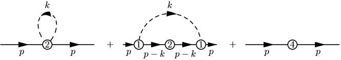
Figure 2: Contributions to the nucleon self energy at ${\cal O}(q^{4})$. The number $n$ in the interaction blobs refers to ${\cal L}_{\pi N}^{(n)}$. The Lagrangian ${\cal L}_{\pi N}^{(2)}$ does not produce a contribution to the $\pi NN$ vertex.

The quark-mass expansion up to and including ${\cal O}(q^{4})$ is given by

$$m_{N}=m+k_{1}M^{2}+k_{2}M^{3}+k_{3}M^{4}\ln\left(\frac{M}{m}\right)+k_{4}M^{4}+{\cal O}(M^{5}),$$ (13)

where the coefficients $k_{i}$ in the EOMS scheme read [14]

$$k_{1} = -4c_{1},\quad k_{2}=-\frac{3{\texttt{g}_{A}}^{2}}{32\pi F^{2}},\quad k_{3}=-\frac{3}{32\pi^{2}F^{2}m}\left(\texttt{g}_{A}^{2}-8c_{1}m+c_{2}m+4c_{3}m\right),$$

$$k_{4} = \frac{3{\texttt{g}_{A}}^{2}}{32\pi^{2}F^{2}m}(1+4c_{1}m)+\frac{3}{128\pi^{2}F^{2}}c_{2}-\hat{e}_{1}.$$ (14)

Here, $\hat{e}_{1}=16e_{38}+2e_{115}+2e_{116}$ is a linear combination of ${\cal O}(q^{4})$ coefficients [11]. A comparison with the results using the infrared regularization [12] shows that the lowest-order correction ($k_{1}$ term) and those terms which are non-analytic in the quark mass $\hat{m}$ ($k_{2}$ and $k_{3}$ terms) coincide. On the other hand, the analytic $k_{4}$ term ($\sim M^{4}$) is different. This is not surprising; although both renormalization schemes satisfy the power counting specified in Sec. 2.2, the use of different renormalization conditions is compensated by different values of the renormalized parameters.

For an estimate of the various contributions of Eq. (13) to the nucleon mass, we make use of the parameter set

$$c_{1}=-0.9\,m_{N}^{-1},\quad c_{2}=2.5\,m_{N}^{-1},\quad c_{3}=-4.2\,m_{N}^{-1},\quad c_{4}=2.3\,m_{N}^{-1},$$ (15)

which was obtained in Ref. [21] from a (tree-level) fit to the $\pi N$ scattering threshold parameters. Using the numerical values

$$g_{A}=1.267,\quad F_{\pi}=92.4\,\mbox{MeV},\quad m_{N}=m_{p}=938.3\,\mbox{MeV},\quad M_{\pi}=M_{\pi^{+}}=139.6\,\mbox{MeV},$$ (16)

one obtains for the mass of nucleon in the chiral limit (at fixed $m_{s}\neq 0$) [22]:

$$m=m_{N}-\Delta m=[938.3-74.8+15.3+4.7+1.6-2.3\pm 4]\,\mbox{MeV}=(883\pm 4)\,\mbox{MeV}$$ (17)

with $\Delta m=(55.5\pm 4)\,\mbox{MeV}$. Here, we have made use of an estimate for $\hat{e}_{1}M^{4}=(2.3\pm 4)$ MeV obtained from the sigma term $\sigma=(45\pm 8)$ MeV. Note that errors due to higher-order corrections are not taken into account.

3.2 Chiral expansion of the nucleon mass to ${\cal O}(q^{6})$

So far, essentially all of the manifestly Lorentz-invariant calculations have been restricted to the one-loop level. One of the exceptions is the chiral expansion of the nucleon mass which, in the framework of the reformulated infrared regularization, has been calculated up to and including ${\cal O}(q^{6})$ [23, 24]:

$$m_{N}=m+k_{1}M^{2}+k_{2}\,M^{3}+k_{3}M^{4}\ln\frac{M}{\mu}+k_{4}M^{4}+k_{5}M^{5}\ln\frac{M}{\mu}+k_{6}M^{5}+k_{7}M^{6}\ln^{2}\frac{M}{\mu}+k_{8}M^{6}\ln\frac{M}{\mu}+k_{9}M^{6}.$$ (18)

We refrain from displaying the lengthy expressions for the coefficients $k_{i}$ but rather want to discuss a few general implications [24]. Chiral expansions like Eq. (18) currently play an important role in the extrapolation of lattice QCD results to physical quark masses. Unfortunately, the numerical contributions from higher-order terms cannot be calculated so far since, starting with $k_{4}$, most expressions in Eq. (18) contain unknown low-energy coupling constants (LECs) from the Lagrangians of ${\cal O}(q^{4})$ and higher. The coefficient $k_{5}$ is free of higher-order LECs and is given in terms of the axial-vector coupling constant $\texttt{g}_{A}$ and the pion-decay constant $F$:

$$k_{5}=\frac{3\texttt{g}_{A}^{2}}{1024\pi^{3}F^{4}}\,\left(16\texttt{g}_{A}^{2}-3\right).$$

While the values for both $\texttt{g}_{A}$ and $F$ should be taken in the chiral limit, we evaluate $k_{5}$ using the physical values $g_{A}=1.2695(29)$ and $F_{\pi}=92.42(26)$ MeV. Setting $\mu=m_{N}$, $m_{N}=(m_{p}+m_{n})/2=938.92$ MeV, and $M=M_{\pi^{+}}=139.57$ MeV we obtain $k_{5}M^{5}\ln(M/m_{N})=-4.8$ MeV. This amounts to approximately $31$% of the leading non-analytic contribution at one-loop order, $k_{2}M^{3}$.

Figure 3: Pion mass dependence of the term $k_{5}M^{5}\ln(M/m_{N})$ (solid line) for $M<400\,\mbox{MeV}$. For comparison also the term $k_{2}M^{3}$ (dashed line) is shown.

Figure 3 shows the pion mass dependence of the term $k_{5}M^{5}\ln(M/m_{N})$ (solid line) in comparison with the term $k_{2}M^{3}$ (dashed line) for pion masses below $400\,\mbox{MeV}$ which is considered a region where chiral extrapolations are valid (see, e.g., Refs. [25, 29]). We see that already at $M\approx 360\,\mbox{MeV}$ the term $k_{5}M^{5}\ln(M/m_{N})$ becomes as large as the leading non-analytic term at one-loop order, $k_{2}M^{3}$, indicating the importance of the fifth-order terms at unphysical pion masses. The results for the renormalization-scheme-independent terms agree with the heavy-baryon ChPT results of Ref. [30].

3.3 Probing the convergence of perturbative series

The issue of the convergence of perturbative calculations is presently of great interest in the context of chiral extrapolations of baryon properties (see, e.g., Refs. [26, 27, 28]). A possibility of exploring the convergence of perturbative series consists of summing up certain sets of an infinite number of diagrams by solving integral equations exactly and comparing the solutions with the perturbative contributions [29].

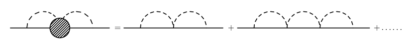
Figure 4: Iterated contribution to the nucleon self energy.

Figure 4 shows a graphical representation of an iterated contribution to the nucleon self energy originating from the Weinberg-Tomozawa term in the $\pi N$ scattering amplitude. The result is of the form [29]

$$\delta m=-\frac{3\texttt{g}_{A}^{2}}{4F^{2}}\frac{N}{D},$$ (19)

where $N$ and $D$ are closed expressions in terms of the loop functions of Eqs. (3) - (5). By expanding Eq. (19) in powers of $1/F^{2}$ one can identify the contributions of each diagram separately. Using the IR renormalization scheme and substituting $m=883$ MeV, $m_{N}=938.3$ MeV, $F=92.4$ MeV, $\texttt{g}_{A}=1.267$ and $M=139.6$ MeV one obtains

$$\delta m=-0.00233530\,{\rm MeV}=\left(-0.00230219-0.00003305-0.00000007+\cdots\right)\,{\rm MeV}\,.$$ (20)

The first term in the perturbative expansion reproduces the non-perturbative result well and the higher-order corrections are clearly suppressed. Figure 5 shows $\delta m$ of Eq. (19) together with the leading contribution (first diagram in Fig. 4) and the leading non-analytic correction to the nucleon mass $\delta m_{3}=-3\,g_{A}^{2}\,M^{3}/(32\,\pi\,F^{2})$ [6] as functions of $M$. As can be seen from this figure, up to $M\sim 500$ MeV the non-perturbative sum of higher-order corrections is suppressed in comparison with the $\delta m_{3}$ term. Also, the leading higher-order contribution reproduces the non-perturbative result quite well. On the other hand, for $M\gtrsim 600$ MeV the higher-order contributions are no longer suppressed in comparison with $\delta m_{3}$.

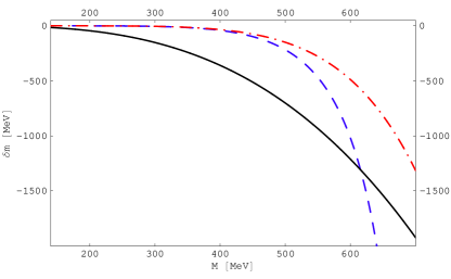
Figure 5: Contributions to the nucleon mass as functions of $M$. Solid line: ${\cal O}(q^{3})$ contribution, dashed line: $\delta m$ of Eq. (19); dashed-dotted line: two-loop diagram of Fig. 4.

3.4 Electromagnetic form factors of the nucleon

Imposing the relevant symmetries such as translational invariance, Lorentz covariance, the discrete symmetries, and current conservation, the nucleon matrix element of the electromagnetic current operator ${\cal J}^{\mu}(x)$ can be parameterized in terms of two form factors,

$$\langle N(p^{\prime},s^{\prime})|{\cal J}^{\mu}(0)|N(p,s)\rangle=\bar{u}(p^{\prime},s^{\prime})\left[F_{1}^{N}(Q^{2})\gamma^{\mu}+i\frac{\sigma^{\mu\nu}q_{\nu}}{2m_{p}}F_{2}^{N}(Q^{2})\right]u(p,s),\quad N=p,n,$$ (21)

where $q=p^{\prime}-p$, $Q^{2}=-q^{2}$, and $m_{p}$ is the proton mass. At $Q^{2}=0$, the so-called Dirac and Pauli form factors $F_{1}$ and $F_{2}$ reduce to the charge and anomalous magnetic moment in units of the elementary charge and the nuclear magneton $e/(2m_{p})$, respectively,

$$F_{1}^{p}(0)=1,\quad F_{1}^{n}(0)=0,\quad F_{2}^{p}(0)=1.793,\quad F_{2}^{n}(0)=-1.913.$$

The Sachs form factors $G_{E}$ and $G_{M}$ are linear combinations of $F_{1}$ and $F_{2}$,

$$G_{E}^{N}(Q^{2})=F_{1}^{N}(Q^{2})-\frac{Q^{2}}{4m_{p}^{2}}F_{2}^{N}(Q^{2}),\quad G_{M}^{N}(Q^{2})=F_{1}^{N}(Q^{2})+F_{2}^{N}(Q^{2}),\quad N=p,n,$$

and, in the non-relativistic limit, their Fourier transforms are commonly interpreted as the distribution of charge and magnetization inside the nucleon.

Calculations in Lorentz-invariant baryon ChPT up to fourth order fail to describe the proton and nucleon form factors for momentum transfers beyond $Q^{2}\sim 0.1\,\mbox{GeV}^{2}$ [31, 32]. Moreover, up to and including ${\cal O}(q^{4})$, the most general effective Lagrangian provides sufficiently many independent parameters such that the empirical values of the anomalous magnetic moments and the charge and magnetic radii are fitted rather than predicted. Figure 6 shows the Sachs form factors in the momentum transfer region $0\,{\rm GeV^{2}}\leq Q^{2}\leq 0.4\,{\rm GeV^{2}}$ in the EOMS scheme and the reformulated infrared regularization [33].

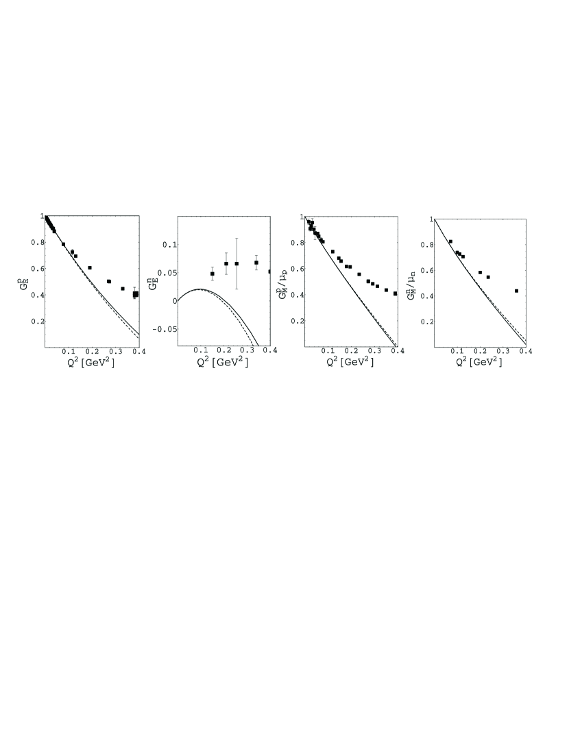
Figure 6: The Sachs form factors of the nucleon in manifestly Lorentz-invariant chiral perturbation theory at ${\cal O}(q^{4})$ without vector mesons. Full lines: results in the extended on-mass-shell scheme; dashed lines: results in infrared regularization. The experimental data are taken from Ref. [34].

In Ref. [31] it was shown that the inclusion of vector mesons can result in the re-summation of important higher-order contributions. In Ref. [33] the electromagnetic form factors of the nucleon up to fourth order have been calculated in manifestly Lorentz-invariant ChPT with vector mesons as explicit degrees of freedom. A systematic power counting for the renormalized diagrams has been implemented using both the extended on-mass-shell renormalization scheme and the reformulated version of infrared regularization. As expected on phenomenological grounds, the quantitative description of the data has improved considerably for $Q^{2}\geq 0.1$ GeV² (see Fig. 7).

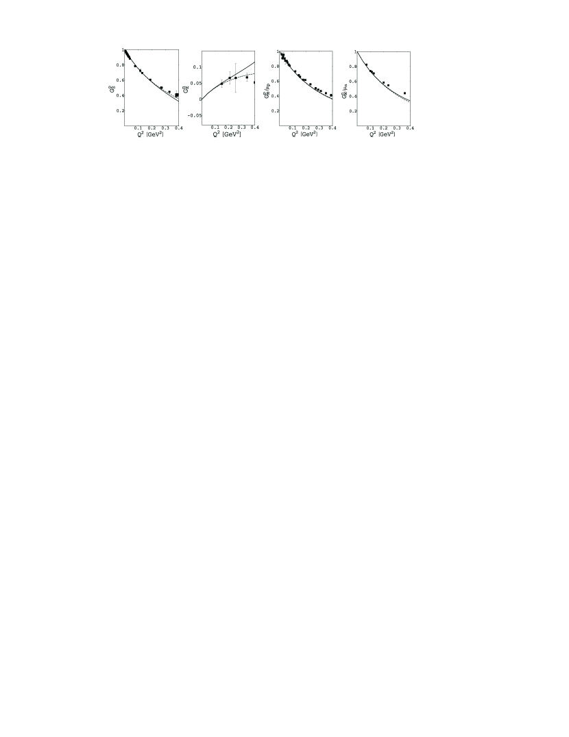
Figure 7: The Sachs form factors of the nucleon in manifestly Lorentz-invariant chiral perturbation theory at ${\cal O}(q^{4})$ including vector mesons as explicit degrees of freedom. Full lines: results in the extended on-mass-shell scheme; dashed lines: results in infrared regularization. The experimental data are taken from Ref. [34].

The small difference between the two renormalization schemes is due to the way how the regular higher-order terms of loop integrals are treated. Numerically, the results are similar to those of Ref. [31]. Due to the renormalization condition, the contribution of the vector-meson loop diagrams either vanishes (IR) or turns out to be small (EOMS). Thus, in hindsight our approach puts the traditional phenomenological vector-meson-dominance model on a more solid theoretical basis. The inclusion of vector-meson degrees of freedom in the present framework results in a reordering of terms which, in an ordinary chiral expansion, would show up at higher orders beyond ${\cal O}(q^{4})$. It is these terms which change the form factor results favorably for larger values of $Q^{2}$. It should be noted, however, that this re-organization proceeds according to well-defined rules so that a controlled, order-by-order, calculation of corrections is made possible.

3.5 Axial and induced pseudoscalar form factors

Assuming isospin symmetry, the most general parametrization of the isovector axial-vector current evaluated between one-nucleon states is given by

$$\langle N(p^{\prime})|A^{\mu,a}(0)|N(p)\rangle=\bar{u}(p^{\prime})\left[\gamma^{\mu}\gamma_{5}G_{A}(Q^{2})+\frac{q^{\mu}}{2m_{N}}\gamma_{5}G_{P}(Q^{2})\right]\frac{\tau^{a}}{2}u(p),$$ (22)

where $q=p^{\prime}-p$, $Q^{2}=-q^{2}$, and $m_{N}$ denotes the nucleon mass. $G_{A}(Q^{2})$ is called the axial form factor and $G_{P}(Q^{2})$ is the induced pseudoscalar form factor. The value of the axial form factor at zero momentum transfer is defined as the axial-vector coupling constant, $g_{A}=G_{A}(Q^{2}=0)=1.2695(29)$, and is quite precisely determined from neutron beta decay. The $Q^{2}$ dependence of the axial form factor can be obtained either through neutrino scattering or pion electroproduction (see, e.g., Ref. [35]). The induced pseudoscalar form factor $G_{P}(Q^{2})$ has been investigated in ordinary and radiative muon capture as well as pion electroproduction (see Ref. [36] for a review).

In Ref. [37] the form factors $G_{A}$ and $G_{P}$ have been calculated in manifestly Lorentz-invariant baryon ChPT up to and including order ${\cal O}(q^{4})$. In addition to the standard treatment including the nucleon and pions, the axial-vector meson $a_{1}(1260)$ has also been considered as an explicit degree of freedom. The inclusion of the axial-vector meson effectively results in one additional low-energy coupling constant which has been determined by a fit to the data for $G_{A}(Q^{2})$. The inclusion of the axial-vector meson results in an improved description of the experimental data for $G_{A}$ (see Fig. 8), while the contribution to $G_{P}$ is small.

Figure 8: Left panel: Axial form factor $G_{A}$ in manifestly Lorentz-invariant ChPT at ${\cal O}(q^{4})$ including the axial-vector meson $a_{1}(1260)$ explicitly. Full line: result in infrared renormalization, dashed line: dipole parametrization. The experimental data are taken from Ref. [35]. Right panel: The induced pseudoscalar form factor $G_{P}$ in manifestly Lorentz-invariant ChPT at ${\cal O}(q^{4})$ including the axial-vector meson $a_{1}(1260)$ explicitly. Full line: result with axial-vector meson; dashed line: result without axial-vector meson. One can clearly see the dominant pion pole contribution at $Q^{2}\approx-M_{\pi}^{2}$.

4 Summary and conclusion

In the baryonic sector new renormalization conditions have reconciled the manifestly Lorentz-invariant approach with the standard power counting. We have discussed some results of a two-loop calculation of the nucleon mass. The inclusion of vector and axial-vector mesons as explicit degrees of freedom leads to an improved phenomenological description of the electromagnetic and axial form factors, respectively. Work on the application to electromagnetic processes such as Compton scattering and pion production is in progress.

I would like to thank D. Djukanovic, T. Fuchs, J. Gegelia, G. Japaridze, and M. R. Schindler for the fruitful collaboration on the topics of this talk. This work was made possible by the financial support from the Deutsche Forschungsgemeinschaft (SFB 443 and SCHE 459/2-1) and the EU Integrated Infrastructure Initiative Hadron Physics Project (contract number RII3-CT-2004-506078).

References

- [1] S. Weinberg, Physica A 96, 327 (1979).
- [2] J. Gasser and H. Leutwyler, Annals Phys. 158, 142 (1984).
- [3] S. Scherer, Adv. Nucl. Phys. 27, 277 (2003).
- [4] J. Bijnens, Prog. Part. Nucl. Phys. 58, 521 (2007).
- [5] S. Scherer, Prog. Part. Nucl. Phys. (2009), doi:10.1016/j.ppnp.2009.08.002.
- [6] J. Gasser, M. E. Sainio, and A. Švarc, Nucl. Phys. B307, 779 (1988).
- [7] S. Weinberg, The Quantum Theory of Fields. Vol. 1: Foundations, Cambridge University Press, Cambridge, 1995.
- [8] J. C. Collins, Renormalization, Cambridge University Press, Cambridge, 1984.
- [9] E. Jenkins and A. V. Manohar, Phys. Lett. B 255, 558 (1991).
- [10] V. Bernard, N. Kaiser, J. Kambor, and U.-G. Meißner, Nucl. Phys. B388, 315 (1992).
- [11] N. Fettes, U. G. Meißner, M. Mojžiš, and S. Steininger, Annals Phys. 283, 273 (2000). [Erratum-ibid. 288, 249 (2001)].
- [12] T. Becher and H. Leutwyler, Eur. Phys. J. C 9, 643 (1999).
- [13] J. Gegelia and G. Japaridze, Phys. Rev. D 60, 114038 (1999).
- [14] T. Fuchs, J. Gegelia, G. Japaridze, and S. Scherer, Phys. Rev. D 68, 056005 (2003).
- [15] J. Gegelia, G. S. Japaridze, and K. S. Turashvili, Theor. Math. Phys. 101, 1313 (1994) [Teor. Mat. Fiz. 101, 225 (1994)].
- [16] T. Fuchs, M. R. Schindler, J. Gegelia, and S. Scherer, Phys. Lett. B 575, 11 (2003).
- [17] C. Hacker, N. Wies, J. Gegelia, and S. Scherer, Phys. Rev. C 72, 055203 (2005).
- [18] M. R. Schindler, J. Gegelia, and S. Scherer, Phys. Lett. B 586, 258 (2004).
- [19] M. R. Schindler, J. Gegelia, and S. Scherer, Nucl. Phys. B682, 367 (2004).
- [20] D. Djukanovic, J. Gegelia, A. Keller, and S. Scherer, Phys. Lett. B 680, 235 (2009).
- [21] T. Becher and H. Leutwyler, JHEP 0106, 017 (2001).
- [22] T. Fuchs, J. Gegelia, and S. Scherer, Eur. Phys. J. A 19, 35 (2004).
- [23] M. R. Schindler, D. Djukanovic, J. Gegelia, and S. Scherer, Phys. Lett. B 649, 390 (2007).
- [24] M. R. Schindler, D. Djukanovic, J. Gegelia, and S. Scherer, Nucl. Phys. A803, 68 (2008).
- [25] U.-G. Meißner, PoS LAT2005, 009-1 (2006).
- [26] D. B. Leinweber, A. W. Thomas, and R. D. Young, Phys. Rev. Lett. 92, 242002 (2004).
- [27] M. Procura, T. R. Hemmert, and W. Weise, Phys. Rev. D 69, 034505 (2004).
- [28] S. R. Beane, Nucl. Phys. B695, 192 (2004).
- [29] D. Djukanovic, J. Gegelia, and S. Scherer, Eur. Phys. J. A 29, 337 (2006).
- [30] J. A. McGovern and M.C. Birse, Phys. Lett. B 446, 300 (1999).
- [31] B. Kubis and U.-G. Meißner, Nucl. Phys. A679, 698 (2001).
- [32] T. Fuchs, J. Gegelia and S. Scherer, J. Phys. G 30, 1407 (2004).
- [33] M. R. Schindler, J. Gegelia, and S. Scherer, Eur. Phys. J. A 26, 1 (2005).
- [34] J. Friedrich and Th. Walcher, Eur. Phys. J. A 17, 607 (2003).
- [35] V. Bernard, L. Elouadrhiri, and U.-G. Meißner, J. Phys. G 28, R1 (2002).
- [36] T. Gorringe and H. W. Fearing, Rev. Mod. Phys. 76, 31 (2004).
- [37] M. R. Schindler, T. Fuchs, J. Gegelia, and S. Scherer, Phys. Rev. C 75, 025202 (2007).