Relic Gravitational Waves with A Running Spectral Index and Its Constraints at High Frequencies

We study the impact of a running index $\alpha_{t}$ on the spectrum of relic gravitational waves (RGWs) over the whole range of frequency $(10^{-18}\sim 10^{10})$ Hz and reveal its implications in RGWs detections and in cosmology. Analytical calculations show that, although the spectrum of RGWs on low frequencies is less affected by $\alpha_{t}\neq 0$, but, on high frequencies, the spectrum is modified substantially. Investigations are made toward potential detections of the $\alpha_{t}$-modified RGWs for several kinds of current and planned detectors. The Advanced LIGO will likely be able to detect RGWs with $\alpha_{t}\geq 0$ for inflationary models with the inflation index $\beta=-1.956$ and the tensor-scalar ratio $r=0.55$. The future LISA can detect RGWs for a much broader range of ($\alpha_{t}$, $\beta$, $r$), and will have a better chance to break a degeneracy between them. Constraints on $\alpha_{t}$ are estimated from several detections and cosmological observations. Among them, the most stringent one is from the bound of the Big Bang nucleosynthesis (BBN), and requires $\alpha_{t}<0.008$ rather conservatively for any reasonable ($\beta$, $r$), preferring a nearly power-law spectrum of RGWs. In light of this result, one would expect the scalar running index $\alpha_{s}$ to be of the same magnitude as $\alpha_{t}$, if both RGWs and scalar perturbations are generated by the same scalar inflation.

PACS numbers: 04.30.-w, 04.80.Nn, 98.80.Cq

1. Introduction

Inflationary models predict a stochastic background of relic gravitational waves (RGWs) [1, 2, 3, 4, 5, 6], whose spectrum depends upon the initial condition when they were generated. After that, only the expansion of spacetime background will substantially affect its evolution behavior in a determined fashion, since the interaction of RGWs with other cosmic components is typically very weak. Therefore, RGWs carry a unique information of the early Universe, and serve as a probe into the Universe much earlier than the cosmic microwave background (CMB).

Unlike gravitational waves radiated by usual astrophysical process, RGWs exist everywhere and anytime, and, moreover, its spectrum spreads over a broad range of frequency, $(10^{-18}\sim 10^{10})$ Hz. Therefore, RGWs are one of the major scientific goals of various GW detectors, including the ground-based interferometers, such as the ongoing LIGO [7], Advanced LIGO [8], VIRGO [9], GEO [10], and the space interferometers, such as the future LISA [11, 12], DECIGO [13], and ASTROD [14], the cryogenic resonant bar detectors, such as EXPLORER [15], NAUTILUS [16], the cavity detectors MAGO [17], the waveguide detector [18], and the proposed Gaussian maser beam detector at GHz[19]. Besides, a long period of observations of pulsar arrival times can be used as GW detectors at nanoHertz [20, 21], such as PPTA [22]. Furthermore, the very low frequency portion of RGWs also contribute to the CMB anisotropies and polarizations [23], yielding a magnetic type polarization of CMB as a distinguished signal of RGWs. WMAP [24, 25, 26, 27, 28, 29, 30], Planck [31], and the proposed CMBpol [32] are of this type. Therefore, the detailed information of RGWs is much desired both for the detection of RGWs itself and for cosmology as well.

The spectrum of RGWs depends on several physical factors. After being generated, RGWs will be affected by a sequence of stages of cosmic expansion, including the current acceleration [4], also by physical processes in the early Universe, such as the neutrino free-streaming [33, 34, 35], the QCD transition, and the $e^{+}e^{-}$ annihilation [36, 37], etc. But, over all, it depends most sensitively upon the initial condition, which includes the initial amplitude, the spectral index $\beta$, and the running index $\alpha_{t}$, as well. These parameters are predicted by specific models of inflation scenarios [4].

In this paper, based on our previous analytic work of RGWs [4, 35, 37], we will study the modifications by a non-zero $\alpha_{t}$, together with $\beta$, upon the spectrum, and explore its implications for gravitational wave detections. By specifying the scale factor for various expanding stages and by a normalization in light of CMB temperature anisotropies of WMAP 5-year [28, 29, 30], the analytic spectrum $h(k,\tau_{H})$ of RGWs with dependence on $\alpha_{t}$ and $\beta$ will be demonstrated. Although a small $\alpha_{t}$ seems to have insignificant influences upon the spectrum of RGWs on very low frequencies, it will cause increasingly substantial modifications upon the spectrum on higher frequencies. This inevitably leads to far-reaching consequences to RGWs detection, since most of detectors are, or will be, operating at various medium and high frequencies, from around $10^{-9}$ Hz up to around $10^{9}$ Hz. The previously estimated constraints on RGWs should be revised in the presence of $\alpha_{t}$ accordingly. To this end, comparisons will be carried out between the theoretical spectrum of RGWs and the sensitivity of various ongoing and forthcoming GW detectors. Thereby, constraints on $\alpha_{t}$ will be derived and their implications in cosmology will be discussed.

The outline of this paper is as follows. In section 2, the scale factor $a(\tau)$ is specified for consecutive stages of cosmic expansion, and the construction is briefly reviewed for the analytical solution of the RGWs. In section 3, we present the resulting spectrum of RGWs with a scalar running index $\alpha_{t}$ and demonstrate the induced modifications. In section 4, comparisons are made between the calculated RGWs and the sensitivity of several kinds of ongoing and planned GW detectors, thereby, constraints on RGWs are obtained and implications in cosmology are discussed. In this paper we use unit with $c=\hbar=k_{B}=1$.

2. Analytical Solution of RGWs in Expanding Universe

For a spatially flat ($k=0$) universe the Robertson-Walker spacetime has a metric

$$ds^{2}=a^{2}(\tau)[-d\tau^{2}+\delta_{ij}dx^{i}dx^{j}],$$ (1)

where $\tau$ is the conformal time, and the scale factor $a(\tau)$ is determined by the Friedmann equation

$$(\frac{a^{\prime}}{a^{2}})^{2}=\frac{8\pi G}{3}\rho,$$ (2)

where ${}^{\prime}\equiv d/d\tau$. From the very early inflation up to the present accelerating expansion, $a(\tau)$ can be described by the following successive stages [2, 4]:

The inflationary stage:

$$a(\tau)=l_{0}|\tau|^{1+\beta},\,\,\,\,-\infty<\tau\leq\tau_{1},$$ (3)

where the inflation index $\beta$ is an important model parameter, related to the spectral index $n_{s}$ of primordial perturbation via $n_{s}=2\beta+5$. The special case of $\beta=-2$ corresponds the exact de Sitter expansion. But both the model-predicted and the observed results, such as WMAP, indicate that the value of $\beta$ can differ slightly from $-2$. In our presentation, $\beta=-2.015$ and $\beta=-1.956$, corresponding to $n_{s}=0.97$ and $n_{s}=1.089$ respectively, are also taken for illustration.

The reheating stage [35, 37]:

$$a(\tau)=a_{z}|\tau-\tau_{p}|^{1+\beta_{s}},\,\,\,\,\tau_{1}\leq\tau\leq\tau_{s}.$$ (4)

As a reheating model parameter, we will mostly take $\beta_{s}=-0.3$.

The radiation-dominant stage :

$$a(\tau)=a_{e}(\tau-\tau_{e}),\,\,\,\,\tau_{s}\leq\tau\leq\tau_{2}.$$ (5)

The matter-dominant stage:

$$a(\tau)=a_{m}(\tau-\tau_{m})^{2},\,\,\,\,\tau_{2}\leq\tau\leq\tau_{E}.$$ (6)

The accelerating stage up to the present time $\tau_{H}$ [4]:

$$a(\tau)=l_{H}|\tau-\tau_{a}|^{-\gamma},\,\,\,\,\tau_{E}\leq\tau\leq\tau_{H},$$ (7)

where $\gamma$ is a $\Omega_{\Lambda}$-dependent parameter. For instance, $\gamma\simeq 1.06$ for $\Omega_{\Lambda}=0.65$, and $\gamma\simeq 1.044$ for $\Omega_{\Lambda}=0.75$ [35]. To be specific, we take $\gamma\simeq 1.044$ and $\Omega_{\Lambda}=0.75$ in this paper.

In Eqs. (3) – (7), the five instances of time, $\tau_{1}$, $\tau_{s}$, $\tau_{2}$, $\tau_{E}$, and $\tau_{H}$, separate the different stages, and can be determined by the relations [35]: $\frac{a(\tau_{s})}{a(\tau_{1})}=300$ for the reheating stage, $\frac{a(\tau_{2})}{a(\tau_{s})}=10^{24}$ for the radiation stage, $\frac{a(\tau_{E})}{a(\tau_{2})}=\frac{a(\tau_{H})}{a(\tau_{2})}\frac{a(\tau_{E})}{a(\tau_{H})}=3454\frac{a(\tau_{E})}{a(\tau_{H})}$ for the matter stage, and $\frac{a(\tau_{H})}{a(\tau_{E})}=(\frac{\Omega_{\Lambda}}{\Omega_{m}})^{1/3}$ for the present accelerating stage, and $\tau_{H}$ is to be fixed by the normalization

$$|\tau_{H}-\tau_{a}|=1.$$ (8)

In the expressions of $a(\tau)$, there are twelve parameters, among which $\beta$, $\beta_{s}$ and $\gamma$ are imposed as the model parameters. By the continuity of $a(\tau)$ and of $a(\tau)^{\prime}$ at the four instances $\tau_{1}$, $\tau_{s}$, $\tau_{2}$ and $\tau_{E}$, one can fix other eight parameters. The remaining $l_{H}$ can be fixed by

$$l_{H}=\gamma/H_{0},$$ (9)

where $H_{0}$ is the present Hubble constant. We will take the Hubble parameter $h_{0}\simeq 0.71$. Thus $a(\tau)$ is completely fixed [35].

In the present universe the physical frequency for a conformal wavenumber $k$ is given by

$$\nu=\frac{k}{2\pi a(\tau_{H})}=\frac{k}{2\pi l_{H}}.$$ (10)

The comoving wavenumber $k_{H}$ corresponding to a wavelength of Hubble radius $1/H_{0}$ at present is given by

$$k_{H}=\frac{2\pi a(\tau_{H})}{1/H_{0}}=2\pi\gamma,$$ (11)

and another wavenumber which will be used is

$$k_{E}\equiv\frac{2\pi a(\tau_{E})}{1/H(\tau_{E})}={k_{H}}(\Omega_{m}/\Omega_{\Lambda})^{1/3\gamma},$$ (12)

whose corresponding wavelength at the time $\tau_{E}$ is equal to the Hubble radius $1/H(\tau_{E})$ at that moment. Note that, in Eq. (12) we have made corrections to that in Ref. [35].

In the presence of the gravitational waves, the perturbed metric is

$$ds^{2}=a^{2}(\tau)[-d\tau^{2}+(\delta_{ij}+h_{ij})dx^{i}dx^{j}],$$ (13)

where the tensorial perturbation $h_{ij}$ is traceless $h^{i}_{\,\,i}=0$ and transverse $h_{ij,j}=0$. It can be decomposed into the Fourier $k$-modes and into the polarization states, denoted by $\sigma$, as

$$h_{ij}(\tau,{\bf x})=\sum_{\sigma=\times,+}\int\frac{d^{3}k}{(2\pi)^{3}}\epsilon^{\sigma}_{ij}h_{k}^{(\sigma)}(\tau)e^{i\bf{k}\cdot{x}},$$ (14)

where $h_{-k}^{(\sigma)*}(\tau)=h_{k}^{(\sigma)}(\tau)$ ensuring that $h_{ij}$ be real, $\epsilon^{\sigma}_{ij}$ is the polarization tensor. In terms of the mode $h^{(\sigma)}_{k}$, the wave equation is

$$h^{(\sigma)}_{k}{{}^{\prime\prime}}(\tau)+2\frac{a^{\prime}(\tau)}{a(\tau)}h^{(\sigma)}_{k}{{}^{\prime}}(\tau)+k^{2}h^{(\sigma)}_{k}(\tau)=0.$$ (15)

Assuming each polarization, $\times$, $+$, $h^{(\sigma)}_{k}(\tau)$ has the same statistical properties, the super index $(\sigma)$ can be dropped As listed in Eq.(3) through Eq.(7), the scale factor has a power-law form

$$a(\tau)\propto\tau^{\alpha},$$ (16)

and the solution to Eq.(15) is a linear combination of Bessel and Neumann functions

$$h_{k}(\tau)=\tau^{\frac{1}{2}-\alpha}\big{[}C_{1}J_{\alpha-\frac{1}{2}}(k\tau)+C_{2}N_{\alpha-\frac{1}{2}}(k\tau)\big{]},$$ (17)

where the constants $C_{1}$ and $C_{2}$ for each stage are determined by the continuity of $h_{k}$ and of $h^{\prime}_{k}$ at the joining points $\tau_{1},\tau_{s},\tau_{2}$ and $\tau_{E}$ [4, 35, 37]. Therefore, the analytical solution of RGWs is completely fixed, once the initial condition during the inflation is given.

For the inflationary stage, one has

$$h_{k}(\tau)=A_{0}l_{0}^{-1}|\tau|^{-(\frac{1}{2}+\beta)}\big{[}A_{1}J_{\frac{1}{2}+\beta}(k\tau)+A_{2}J_{-(\frac{1}{2}+\beta)}(k\tau)\big{]},\,\,\,\,\,\,-\infty<\tau\leq\tau_{1},$$ (18)

where the $k$-independent constant $A_{0}$ determines the initial amplitude, and

$$A_{1}=-\frac{i}{\cos\beta\pi}\sqrt{\frac{\pi}{2}}e^{i\pi\beta/2},\,\,\,\,\,A_{2}=iA_{1}e^{-i\pi\beta},$$ (19)

are taken [38, 4, 35], so that in the high frequency limit $\lim_{k\rightarrow\infty}h_{k}(\tau)\propto e^{-ik\tau}$ the adiabatic vacuum is achieved [39]. In the long wave-length limit, $k\tau\ll 1$, the $k$-dependence of $h_{k}(\tau)$ is given by

$$h_{k}(\tau)\propto J_{\frac{1}{2}+\beta}(k\tau)\propto k^{\frac{1}{2}+\beta}.$$ (20)

3. Spectrum of RGWs with a Running Index

The spectrum of RGWs $h(k,\tau)$ at a time $\tau$ is defined by the following equation:

$$\int_{0}^{\infty}h^{2}(k,\tau)\frac{dk}{k}\equiv\langle 0|h^{ij}(\textbf{x},\tau)h_{ij}(\textbf{x},\tau)|0\rangle,$$ (21)

where the right-hand side is the expectation value of the $h^{ij}h_{ij}$. Calculation yields the spectrum as follows

$$h(k,\tau)=\frac{\sqrt{2}}{\pi}k^{3/2}|h_{k}(\tau)|.$$ (22)

Note that this expression has a factor $\sqrt{2}$ in place the factor $2$ in Ref. [35]. As the initial condition, the primordial spectrum of RGWs at the time $\tau_{i}$ of the horizon-crossing during the inflation is usually taken to be a power-law form [2, 4, 35]:

$$h(k,\tau_{i})=A(\frac{k}{k_{H}})^{2+\beta},$$ (23)

where the index $\beta\simeq-2$ for a nearly scale-invariant spectrum, and $A$ is proportional to $A_{0}$ in Eq.(18). In principle, both $\beta$ and $A$ are determined by the specific inflationary model. Here we take them as two independent parameters. In literature, the following notation is often used for the RGWs spectrum [24, 28]

$$\Delta^{2}_{h}(k)\equiv h^{2}(k,\tau_{i})=\Delta^{2}_{h}(k_{0})\left(\frac{k}{k_{0}}\right)^{n_{t}},$$ (24)

where $k_{0}$ is a conformal pivot wavenumber, whose corresponding physical wavenumber is $k^{p}_{0}=k_{0}/a(\tau_{H})$. For WMAP, the pivot $k_{0}^{p}=0.002$ Mpc^-1 is taken [24, 25, 28]. Comparing Eqs. (23) and (24) yields

$$n_{t}=2\beta+4$$ (25)

and

$$A=\Delta_{h}(k_{0})\left(\frac{k_{H}}{k_{0}}\right)^{2+\beta}.$$ (26)

For each cosmological model with $k_{H}$ and $\beta$ being given, $\Delta_{h}(k_{0})$ determines $A$. More often in literature, a tensor-to-scalar ratio $r$ is introduced [24]

$$r\equiv\frac{\Delta^{2}_{h}(k_{0})}{\Delta^{2}_{\Re}(k_{0})},$$ (27)

where $\Delta^{2}_{\Re}(k_{0})$ is the amplitude of the curvature spectrum at $k=k_{0}$, and has been fixed $\Delta^{2}_{\Re}(k_{0})=(2.41\pm 0.11)\times 10^{-9}$ by WMAP5 Mean [30], and $\Delta^{2}_{\Re}(k_{0})=(2.445\pm 0.096)\times 10^{-9}$ by WMAP5+BAO+SN Mean [28]. Note that this scalar amplitude has been “fixed” only after the assumption that the data do not contain gravitational waves, i.e. $r=0$. Here we use $r$ as a convenient representation of the amplitude normalization of $\Delta_{h}(k_{0})$ at $k_{0}$, i.e., $\Delta_{h}(k_{0})=4.94\times 10^{-5}r^{1/2}$. Thus, Eq.(26) is rewritten as the following

$$A=4.94\times 10^{-5}r^{\frac{1}{2}}(\frac{k_{H}}{k_{0}})^{2+\beta}.$$ (28)

At present, only observational constraints on $r$ have been given by WMAP [28, 29, 30]. To be specific in our presentation, $r=0.55$ and $r=0.22$ will be taken, respectively.

In general, the spectra of primordial perturbations, both scalar and tensorial, deviate from the exact power-law form except when the inflation potential is an exponential. As an extension, one usually consider the following form of power spectra [40, 41]

$$\Delta^{2}_{\Re}(k)=\Delta^{2}_{\Re}(k_{0})\left(\frac{k}{k_{0}}\right)^{-1+n_{s}(k_{0})+\frac{1}{2}\alpha_{s}\ln{(k/k_{0})}},$$ (29)

$$\Delta^{2}_{h}(k)=\Delta^{2}_{h}(k_{0})\left(\frac{k}{k_{0}}\right)^{n_{t}(k_{0})+\frac{1}{2}\alpha_{t}\ln{(k/k_{0})}},$$ (30)

which contain the “running” spectral indices $\alpha_{s}\equiv dn_{s}/d\ln k$ for the scalar perturbations and $\alpha_{t}\equiv dn_{t}/d\ln k$ for the tensorial perturbations. Currently, WMAP has given some preliminary constraint on the scalar index $n_{s}$ and the scalar running index $\alpha_{s}$. At the pivot wavenumber $k^{p}_{0}=k_{0}/a(\tau_{H})=0.002$ Mpc^-1, WMAP1 has given $n_{s}=1.20^{+0.12}_{-0.11}$ and $\alpha_{s}=-0.077^{+0.050}_{-0.052}$ [24]; WMAP3 has given $n_{s}=0.951^{+0.015}_{-0.019}$ and $\alpha_{s}=-0.055^{+0.029}_{-0.035}$ [26]. With a better determination of the third acoustic peak, WMAP5 has given an improved result: $n_{s}=1.087^{+0.072}_{-0.073}$ and $\alpha_{s}=-0.050{\pm 0.034}$ [28]; and WMAP5+BAO+SN has given $n_{s}=1.089^{+0.070}_{-0.068}$ and $\alpha_{s}=-0.053^{+0.027}_{-0.028}$, or $n_{s}=0.970\pm 0.015$ without $\alpha_{s}$ [28]. Compared with $n_{s}$, the value of the scalar running $\alpha_{s}$ is relatively small. Thus WMAP5 data do not significantly prefer a scalar running index [30]. See also Refs. [42] for relevant discussions.

But so far there is no direct observation of the tensorial index $n_{t}$ nor the running index $\alpha_{t}$. In the slow roll inflationary models driven by a single scalar field, the tensorial indices, $n_{t}$ and $\alpha_{t}$, are determined by the inflationary potential and its derivatives, so are the scalar ones, $n_{s}$ and $\alpha_{s}$, as well [40, 41]. There would be relations between the tensorial indices and the scalar ones, if one imposes further a consistency relation. In our context, for generality, we will treat $n_{t}$ and $\alpha_{t}$ as parameters independent of $n_{s}$ and $\alpha_{s}$. Corresponding to Eq.(30), the primordial spectrum in Eq. (23) is modified to

$$h(k,\tau_{i})=A(\frac{k}{k_{H}})^{2+\beta}A_{\alpha_{t}}(k)$$ (31)

where the the extra factor

$$A_{\alpha_{t}}(k)\equiv(\frac{k}{k_{0}})^{\frac{1}{4}\alpha_{t}\ln{(k/k_{0})}}$$ (32)

is the $\alpha_{t}-$induced deviation from the simple power-law spectrum, reflecting an extra bending. With the help of Eq.(28), this is

$$h(k,\tau_{i})=\Delta_{\Re}(k_{0}){r}^{\frac{1}{2}}(\frac{k}{k_{0}})^{2+\beta}A_{\alpha_{t}}(k).$$ (33)

For a tiny $\alpha_{t}=0.01$, in the very low frequency range, from $\nu=\nu_{0}=3\times 10^{-18}$ Hz to $\nu=3\times 10^{-16}$ Hz, $A_{\alpha_{t}}(k)$ goes from 1 to $1.055$, causing only a minor increase in the amplitude by $\leq 5.5\%$. However, at very high frequency, say $\nu=10^{9}$ Hz, $A_{\alpha_{t}}(k)\sim 10^{4}$, enhancing the amplitude by 4 orders of magnitude. This drastic effect requires a detailed investigation into $\alpha_{t}$ and its consequential implications.

As discussed in Refs. [4, 35, 37], at the present time $\tau=\tau_{H}$, the long wavelength modes $h_{k}(\tau)$ with wavenumber $k\leq k_{E}$ are still outside the horizon, their spectrum are still of the form in (33), $h(k,\tau_{H})=h(k,\tau_{i})$. Given this initial condition with a running index, the analytic calculation of the spectrum of RGWs can be carried out straightforwardly, in the same way as the non running case [4, 35]. The only difference in the actual computing procedure is the amplitude normalization of the RGWs spectrum, which can be taken at the wavenumber $k_{E}$, corresponding to a physical frequency $\nu_{E}=k_{E}/2\pi a(\tau_{H})=H_{0}/(1+z_{E})\sim 10^{-18}$ Hz. With the help of Eq.(33), it is given by

$$h(k_{E},\tau_{H})=\Delta_{\Re}(k_{0}){r}^{\frac{1}{2}}(\frac{k_{E}}{k_{0}})^{2+\beta+\frac{1}{4}\alpha_{t}\ln{(k_{E}/k_{0})}}.$$ (34)

In a cosmological model with a given set of $(r,\beta,\alpha_{t})$, the resulting RGWs spectrum $h(\nu,\tau_{H})$ at present is fully determined.

Another important quantity often used in constraining RGWs is its present energy density parameter defined by $\Omega_{gw}=\frac{\rho_{g}}{\rho_{c}}$, where $\rho_{g}=\frac{1}{32\pi G}h_{ij,0}h^{ij}_{,0}$ is the energy density of RGWs, and $\rho_{c}=3H_{0}^{2}/8\pi G$ is the critical energy density. A direct calculation yields [2]

$$\Omega_{gw}=\int_{\nu_{low}}^{\nu_{upper}}\Omega_{g}(\nu)\frac{d\nu}{\nu},$$ (35)

with

$$\Omega_{g}(\nu)=\frac{\pi^{2}}{3}h^{2}(\nu,\tau_{H})\Big{(}\frac{\nu}{\nu_{H}}\Big{)}^{2}$$ (36)

being the dimensionless spectral energy density. From this expression, it is seen that the spectral energy density $\Omega_{g}(\nu)$ and the spectrum $h(\nu,\tau_{H})$ are two equivalent quantities, and $h(\nu,\tau_{H})/\sqrt{2}$ is just the characteristic amplitude, denoted by $h_{c}(f)$ in Ref.[5]. As the cutoffs of frequencies, the lower and upper limit of integration in Eq.(35) can be taken to be $\nu_{low}\simeq 2\times 10^{-18}$ Hz and $\nu_{upper}\simeq 10^{10}$ Hz, respectively [35]. In the case of $\alpha_{t}=0$, the slope of $\Omega_{g}(\nu)$ is fixed by the index $\beta$, and the overall amplitude of $\Omega_{g}(\nu)$ is fixed by $r$, as shown in Fig. 1. In the following, two combinations $(r=0.55,\beta=-1.956)$ and $(r=0.22,\beta=-2.015)$ will often be taken for specific illustrations.

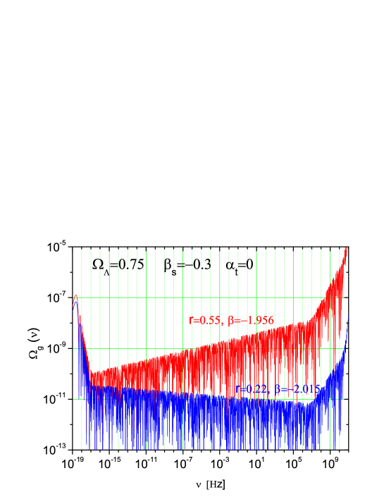
Figure 1: The spectral energy density $\Omega_{g}(\nu)$ with $\alpha_{t}=0$ for two sets of $r$ and $\beta$.

When there is a running index $\alpha_{t}\neq 0$, the slopes of $\Omega_{g}(\nu)$, and of $h(\nu,\tau_{H})$ as well, are affected substantially. Fig. 2 demonstrates $h(\nu,\tau_{H})$ for various values of $\alpha_{t}$ in the model with $r=0.22$ and $\beta=-2.015$. It is seen that a greater $\alpha_{t}$ yields a higher $h(\nu,\tau_{H})$ and that the modifications due to $\alpha_{t}$ increase with the frequency $\nu$. While the effects are small in the low frequency range, they are quite substantial in the high-frequency range. For instance, in going from $\alpha_{t}=-0.01$ to $\alpha_{t}=0.01$, the amplitude of $h(\nu,\tau_{H})$ gets enhanced by $3$ orders of magnitudes at $\nu\simeq 10^{-2}$ Hz falling the range for LISA, $5$ orders at $\nu\simeq 10^{2}$ Hz for LIGO, $6$ orders at $\nu\simeq 10^{4}$ Hz for MAGO [17], and $9$ orders at $\nu\simeq 10^{9}$Hz for the Gauss beam [19]. Equivalently, Fig.3 gives the $\alpha_{t}-$dependence of the spectral energy density $\Omega_{g}(\nu)$, which shows more drastically the variations in high frequencies due to $\alpha_{t}$.

Notice that the ratio $r$, the index $\beta$, and the running index $\alpha_{t}$ in Eq.(31) play different roles in shaping the spectrum of RGWs. $r$ sets the amplitude, $\beta$ fixes the overall slope of the spectrum, and $\alpha_{t}$ gives an extra bending to it. However, in a rather narrow interval of detecting frequencies, $r$, $\beta$, and $\alpha_{t}$ have a degeneracy to certain extent, since a larger value of each of them tends to enhance the amplitude of $h(\nu,\tau_{H})$ in the interval. The narrower the interval is, the stronger the degeneracy will be. Therefore, if a detector is operating in a narrow interval of frequencies, it can only detect RGWs for a combination of parameters $(r,\beta,\alpha_{t})$. Those detectors operating over a broad frequency interval will have a better chance to break the degeneracy.

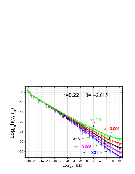
Figure 2: The spectrum of RGWs for various $\alpha_{t}$.

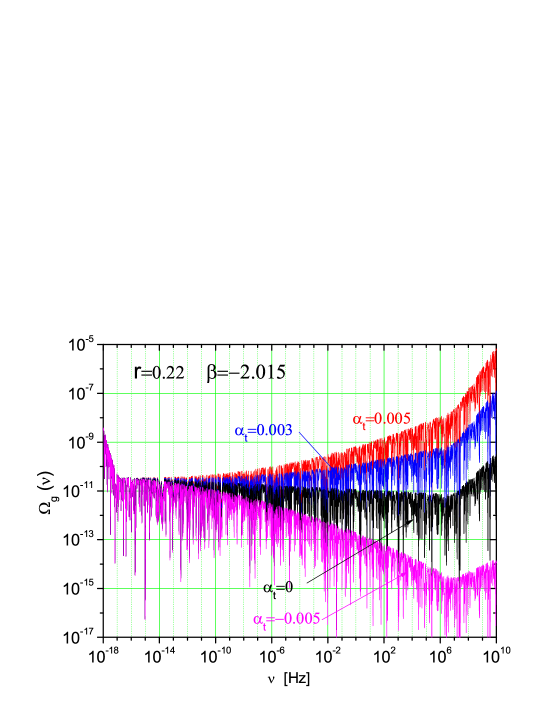
Figure 3: The spectral energy density $\Omega_{g}(\nu)$ for various $\alpha_{t}$.

4. Constraints from Detections and Implications

The $\alpha_{t}$-induced modification of the RGWs spectrum has practical implications for the ongoing and planned GW detections in the medium, and the high-frequency ranges. Some previously estimated constraints on RGWs were based on the theoretical spectrum without a running index [4, 35, 37]. Now these will be subsequently revised to certain extent.

Figure 4 gives the comparison of the sensitivity curves of LIGO [7] and Advanced LIGO [8] with the theoretical spectra of RGWs for various parameters ($r$, $\beta$, $\alpha_{t}$), in the frequency range $(10^{1},10^{4})$ Hz. Note that, in order to compare to the strain sensitivity $\tilde{h}_{f}(\nu)$ [5, 43] of the detectors, the amplitude per root Hz, ${h(\nu,\tau_{H})}/{\sqrt{\nu}}$, has been used. It is seen that, for $r=0.55$ and $\beta=-1.956$, the LIGO I SRD [7] has already put a constraint on the running index: $\alpha_{t}\leq 0.013$. It will yet not be able to detect the signals of RGWs for $r=0.55$, $\beta<-1.956$ and $\alpha_{t}<0.013$. On the other hand, with a substantial improvement in sensitivity, Advanced LIGO will be able to detect the RGWs from models with $r=0.55$ and $\beta>-1.956$ and $\alpha_{t}>0$, but still it will unlikely be able to detect RGWs for $r=0.22$ and $\beta=-2.015$ even for $\alpha_{t}=0.01$ and less.

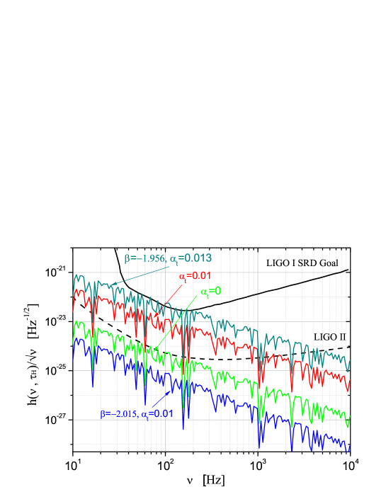
Figure 4: Comparisons of the spectra with the sensitivity of the LIGO I SRD Goal achieved by LIGO S5  [7] and of the Advanced LIGO [8].

Figure 5 is a comparison of the theoretical spectrum with the LISA sensitivity curve [11, 12] for the ratio $S/N=1$ in the frequency range $(10^{-7},10^{0})$ Hz, where one year observation time has been assumed, which corresponds to a frequency bin $\Delta\nu\simeq 3\times 10^{-8}$Hz around each frequency. To make a comparison with the sensitity curve, one needs to rescale the theoretical spectrum $h(\nu,\tau_{H})$ into the rms spectrum $h(\nu,\tau_{H},\Delta\nu)$ in the band $\Delta\nu$ [2, 5],

$$h(\nu,\tau_{H},\Delta\nu)=h(\nu,\tau_{H})\sqrt{\frac{\Delta\nu}{\nu}}.$$ (37)

The plot shows that LISA by its present design will be quite effective in detecting the RGWs around a range of frequencies ($10^{-6},1.5\times 10^{-1}$) Hz. In particular, the plot tells that LISA will be able to detect RGWs for parameters $r\geq 0.22$, $\beta\geq-2.015$, and $\alpha_{t}\geq 0$. Thus, regarding to detection of RGWs, LISA is expected to perform much better than LIGO and Advance LIGO. This advantage is due to the property that the RGWs have a higher amplitude in the range of lower frequencies. The situation is illustrated in Fig.6, in which the sensitivity curves of LIGO and LISA are converted pertinently, in order to compare with the theoretical spectrum $h(\nu,\tau_{H})$. Moreover, regarding to the RGWs detection, the frequency range covered by LISA is very broad, as compared with LIGO. This is because the low frequency portion of LISA sensitivity curve has a slope that is rather close to that of RGWs spectrum in the involved region. This feature of LISA is important and can be instrumental in breaking the $(r,\beta,\alpha_{t})$ degeneracy, as mentioned earlier. Besides, in Fig 6 the sensitivity of planned DECIGO [13] is also presented, together with two more spectra calculated for very low running indices $\alpha_{t}=-0.01$ and $\alpha_{t}=-0.03$, in the model $(r=0.22,\beta=-2.015)$, respectively. DECIGO, if implemented, will be a powerful detector, capable of detecting RGWs with a very low running index $\alpha_{t}>-0.03$.

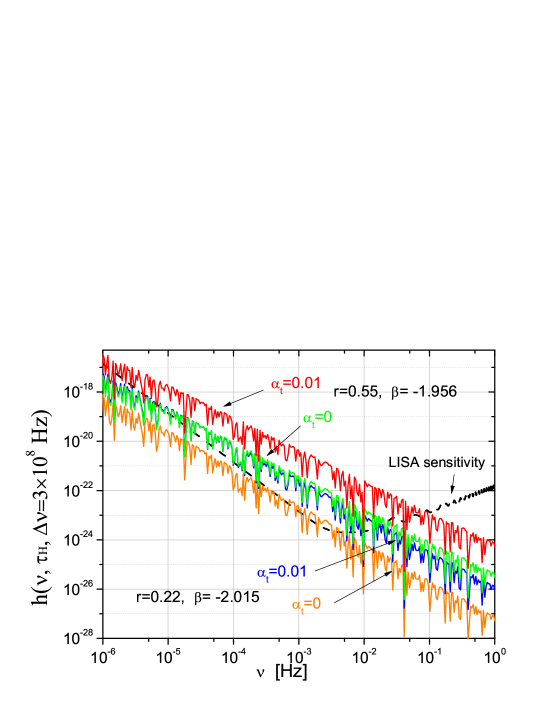
Figure 5: Comparison of the rms spectrum with the LISA sensitivity curve [12].

Figure 6: Comparison of the theoretical spectrum $h(\nu,\tau_{H})$ with the converted sensitivity curve of LIGO, Advanced LIGO, LISA, and DECIGO [13]. The parameters of the four top spectra $h(\nu,\tau_{H})$ are the same as the previous Fig.5.

Fig.7 compares the theoretical spectrum ${h(\nu,\tau_{H})}/{\sqrt{\nu}}$ with the 2005 run sensitivity curve of cryogenic resonant bar detector, EXPLORER in the frequency range $(890,920)$ Hz [15]. It is seen that, even for $\beta=-1.956$ and $\alpha_{t}=-0.01$, RGWs are still far beyond the reach of EXPLORER by three orders of magnitude.

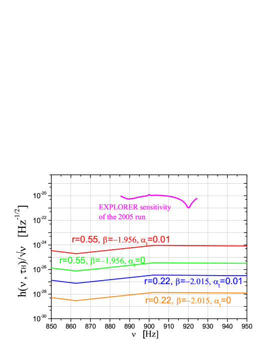
Figure 7: Comparisons of the spectrum with the EXPLORER sensitivity curve [15].

Fig.8 compares the theoretical spectrum ${h(\nu,\tau_{H})}/{\sqrt{\nu}}$ with the sensitivity curve of MAGO, a double spherical cavity detector, around the frequency $4002$ Hz [17]. For $\beta=-1.956$ and $\alpha_{t}=0.01$, RGWs are also beyond the reach of MAGO by three orders of magnitude.

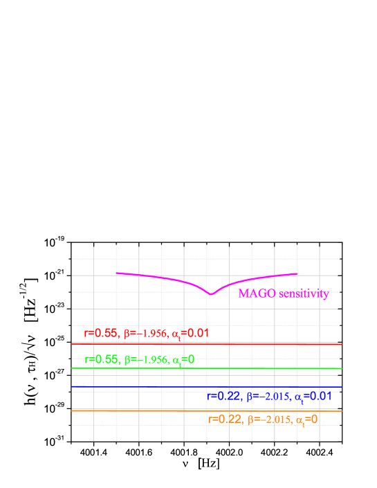
Figure 8: Comparisons of the spectrum with the MAGO sensitivity curve [17].

The proposed Gaussian maser beam detector will operate at a very high frequency, say $\sim 4.5$ GHz [19]. Still the spectrum of RGWs stretches to such high frequencies with enough power, depending on both the energy scale involved in the specific inflationary models and the reheating process. For the designing parameters for the proposed detector, its sensitivity is short by about 6 orders of magnitude. As for the prototype loop waveguide detector [18] operating at a high frequency $100$ MHz, the sensitivity at present is short by much more.

For lack of direct detection of RGWS, cosmological considerations can be more effective in providing the constraints upon the RGWs through its energy density. In particular, the BBN process occurring at a temperature $T\sim$ a few MeV during the early universe is sensitive to the total cosmic energy density, including that of RGWs. An increase in the energy density of RGWs will enhance the freezing temperature of neutrons and hence the light-element abundances. Consequently, this will bring observational constraints on the running index $\alpha_{t}$. The energy density of RGWs should not be too large, otherwise, it will significantly affect the outcome of the BBN process. Measured abundances of light-element constrain the number of additional relativistic species at BBN to an equivalence of $\delta N_{\nu}=1.4$ neutrino degrees of freedom, corresponding to $h_{0}^{2}\Omega_{gw}<7.8\times 10^{-6}$ [44, 5]. Besides, if the initial perturbation amplitude of RGWs is non-adiabatic, as is the case of RGWs being generated during inflation, measurements of the CMB power spectrum also provide a constraint $h_{0}^{2}\Omega_{g}(\nu)<8.4\times 10^{-6}$ in the very low frequency range $\nu=(10^{-15},10^{-10})$ Hz [45], comparable to that from BBN. In constraining the energy density of RGWs, sometimes $\Omega_{g}(\nu)$ and $\Omega_{gw}$ were used interchangeably in literature. But it is at most an approximation, valid only under the condition that the integration interval $d\nu/\nu=d\log\nu\sim 1$ and $\Omega_{g}(\nu)$ is rather flat and smooth. In this paper we distinguish $\Omega_{g}(\nu)$ and $\Omega_{gw}$, and give a more accurate treatment. Using the normalization of Eq.(34) and carrying out the integration in Eq. (35), we obtain the $\alpha_{t}-$dependence of the the energy density parameter $\Omega_{gw}$ in Fig.9 for various values of parameters. Adopting the BBN bound, the constraint on $\alpha_{t}$ is found to be $\alpha_{t}\leq 0.0014$ for $r=0.55$ and $\beta=-1.956$, $\alpha_{t}\leq 0.0056$ for $r=0.22$ and $\beta=-2.015$, and $\alpha_{t}\leq 0.0077$ for $r=0.001$ and $\beta=-2.0$, respectively. One can infer that the constraint $\alpha_{t}<0.008$ for any reasonable set of cosmological parameters. It should be mentioned that, although the BBN bound yields a constraint on RGWs, it does not provides a direct detection of RGWs, so one can only get upper bounds of $\alpha_{t}$.

This rather stringent constraint on $\alpha_{t}$ supports a nearly power-law spectrum of RGWs, and is consistent with the expectation from scalar inflationary models [40]. However, a comparison shows that, the magnitude of $\alpha_{t}$ constrained by the BBN bound is even smaller by one order than the scalar running index $\alpha_{s}$ obtained by WMAP on large scales [24, 26, 28, 30]. If both RGWs and scalar perturbations are generated by the same inflation, one expects $\alpha_{s}$ to be nearly as small as $\alpha_{t}$ for several kinds of smooth scalar potential [40]. In light of the stringent constraint on $\alpha_{t}$, it is hinted that $\alpha_{s}$ should also be rather small. There has been some debate on the significantly non-vanishing scalar running $\alpha_{s}$ [42]. Therefore, it is much desired that constraints on the scalar running index $\alpha_{s}$ be drawn from observations on smaller sales.

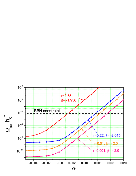
Figure 9: The $\alpha_{t}$-dependence of energy density parameter $\Omega_{gw}$ for various $r$ and $\beta$.

Another kind of stringent constraints on RGWs come from observations of millisecond pulsars, which can serve as a gravitational wave detector in the low frequency range. For instance, by analyzing the uncertainty $\epsilon$ in the arrival timing of pulses for a duration $T$ of observation, the pulsar will be sensitive to gravitational waves $h(\nu,\tau_{H})\sim\epsilon/T$ with $\nu\sim 1/T$. For PSR B1855+09, a bound has been given for RGWs [5, 21]: $\Omega_{g}(\nu_{*})h_{0}^{2}<4.8\times 10^{-9}(\nu/\nu_{*})^{2}$ for $\nu>\nu_{*}$, where $\nu_{*}=4.4\times 10^{-9}$ Hz. Another treatment gives $\Omega_{g}(\nu_{*})h_{0}^{2}<2\times 10^{-9}(\nu/\nu_{*})^{2}$ for $\nu>\nu_{*}$, where $\nu_{*}=1.9\times 10^{-9}$ Hz [46]. Applying this bound to compare with the calculated energy density spectrum $\Omega_{g}(\nu)$, we obtain the constraint on RGWs, shown in Fig.10. For the parameters $r=0.55$ and $\beta=-1.956$, the pulsar detector puts a constraint $\alpha_{t}<0.01$, which is less stringent than the BBN constraint. As an extension of this technique, Parkes Pulsar Timing Array (PPTA) [22, 47] consists of a sample of 20 millisecond pulsars distributed over the entire sky, and correlations in the time residuals of pulsars help to disentangle RGWs signals. After five years of observation, it will improve the sensitivity by about one order over that from a single pulsar and will have a chance to detect RGWs of $r=0.55$, $\beta=-1.956$, and $\alpha_{t}=0$. But for $r=0.22$ and $\beta=-2.015$, the detector will still not be able to detect RGWs for a small value of $\alpha_{t}$.

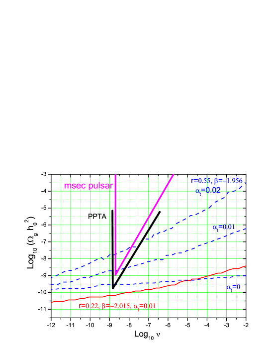
Figure 10: Comparison with the constraint from data of millisecond pulsars [46] and PPTA [47].

In summary, by allowing for a tensorial running index $\alpha_{t}$, the RGWs spectrum $h(\nu,\tau_{H})$ will be significantly affected, particularly in higher frequencies. A positive $\alpha_{t}$ tends to bend the high frequency portion of $h(\nu,\tau_{H})$ to upward, while a negative $\alpha_{t}$ will do the opposite. This has brought about significant consequences to various ongoing and planned detectors, and led to reexaminations of the constraints on parameters of RGWs that were previously estimated for the case $\alpha_{t}=0$. For instance, a small variation of $\alpha_{t}$ from $-0.01$ to $0.01$ will increase the amplitude RGWs by several orders of magnitude, depending on frequencies. It is interesting to note that LISA by its design will be able to detect RGWs with $\alpha_{t}\geq 0$ for the parameters $r=0.22$, $\beta=-2.015$. For an inflationary model with $r=0.55$ and $\beta=-1.956$, the observational constraint is $\alpha_{t}<0.013$ from LIGO S5, $\alpha_{t}<0.01$ from millisecond pulsar PSR B1855+09. The most stringent constraint coming from the BBN bound is $\alpha_{t}<0.008$ as a rather conservative estimate for any reasonable set of cosmological parameter ($\beta$, $r$). The resulting tiny $\alpha_{t}$ prefers the simple inflationary models with a nearly power-law spectrum of RGWs, and would also hint a rather small scalar running index $\alpha_{s}$ within scalar inflationary models. It is also found that there is a degeneracy of $\alpha_{t}$ with $\beta$ and $r$ in a narrow interval of detection frequency. Detectors working in a broad frequency range, such as LISA, may have a better chance in breaking the degeneracy.

ACKNOWLEDGMENT: M. L. Tong’s work has been partially supported by Graduate Student Research Funding from USTC. Y. Zhang’s work has been supported by the CNSF No. 10773009, SRFDP, and CAS.

References

- [1] L. P. Grishchuk, Sov.Phys.JETP 40, 409 (1975); Class.Quant.Grav.14, 1445 (1997);
- [2] L.P. Grishchuk, in Lecture Notes in Physics, Vol.562, p.167, Springer-Verlag, (2001), arXiv: gr-qc/0002035; arXiv: gr-qc/0707.3319.
- [3] A.A. Starobinsky, JEPT Lett. 30, 682 (1979); Sov. Astron. Lett. 11, 133 (1985); V.A. Rubakov, M. Sazhin, and A. Veryaskin, Phys. Lett. B 115, 189 (1982); R. Fabbri and M.D. Pollock, Phys. Lett. B 125, 445 (1983); L. F. Abbott and M.B. Wise, Nucl. Phys. B 244, 541 (1984); B. Allen, Phys. Rev. D 37, 2078 (1988); V. Sahni, Phys. Rev. D 42, 453 (1990); H. Tashiro, T. Chiba, and M. Sasaki, Class. Quant. Grav. 21, 1761 (2004); A. B. Henriques, Class. Quant. Grav. 21, 3057 (2004); W. Zhao and Y. Zhang, Phys. Rev. D 74, 043503 (2006).
- [4] Y. Zhang et al., Class. Quant. Grav. 22, 1383 (2005); Chin. Phys. Lett. 22, 1817 (2005); Class. Quant. Grav. 23, 3783 (2006).
- [5] M. Maggiore, Phys. Rept. 331, 283 (2000).
- [6] M. Giovannini, arXiv:0901.3026[astro-ph].
- [7] http://www.ligo.caltech.edu/.
- [8] http://www.ligo.caltech.edu/advLIGO/.
- [9] A. Freise, et al., Class. Quant. Grav. 22, S869 (2005); http://www.virgo.infn.it/.
- [10] B. Willke, et al., Class. Quant. Grav. 19, 1377 (2002); http://geo600.aei.mpg.de/; http://www.geo600.uni-hannover.de/geocurves/.
- [11] http://lisa.nasa.gov/; http://www.lisa.caltech.edu/.
- [12] http://www.srl.caltech.edu/~shane/sensitivity/MakeCurve.html.
- [13] N. Seto, S. Kawamura, and T. Nakamura, Phys. Rev. Lett. 87, 221103 (2001).
- [14] W. T. Ni, S. Shiomi, and A. C. Liao, Class. Quant. Grav. 21, S641 (2004).
- [15] P. Astone, et al., Class. Quant. Grav. 25, 114028 (2008).
- [16] P. Astone, et al., Astropart. Phys. 7, 231 (1997); Class. Quant. Grav. 25, 184012 (2008).
- [17] R. Ballatini, et al., arXiv:gr-qc/0502054, INFN Technical Note INFN/TC-05/05, (2005).
- [18] A.M. Cruise, Class.Quant.Grav. 17, 2525 (2000) ; A.M. Cruise and R.M.J. Ingley, Class. Quant. Grav. 22, S479 (2005); Class. Quant. Grav. 23, 6185 (2006); M.L. Tong and Y. Zhang, Chin. J. Astron. Astrophys. 8, 314 (2008).
- [19] F.Y. Li, M.X. Tang and D.P. Shi, Phys. Rev. D 67, 104008 (2003); F.Y. Li et al., Eur. Phys. J. C 56, 407 (2008); M.L. Tong, Y. Zhang, and F.Y. Li, Phys. Rev. D 78, 024041 (2008).
- [20] M.V. Sazhin, Sov. Straon. 22, 36 (1978); S. Detweiler, Astrophys. J. 234, 1100 (1979); R.W. Romani and J.H. Taylor, Astrophys. J. 265, L35 (1983); R.W. Hellings and G.S. Downs, Astrophys. J. 265, L39 (1983).
- [21] V.M. Kaspi, J.H. Taylor, and M.F. Ryba, ApJ. 428, 712 (1994); S.E. Thorsett and R.J. Dewey, Phys. Rev. D 53, 3468 (1996).
- [22] G. Hobbs, PASA 22, 179 (2005), arXiv:astro-ph/0412153; Class. Quant. Grav. 25, 114032 (2008); J. Phys. Conf. Ser. 122, 012003 (2008); G. Hobbs, et al., arXiv:0812.2721[astro-ph]; F.A. Jenet, et al., Astrophys. J. 653, 1571 (2006); R.N. Manchester, AIP Conf. Series. Proc. 983, 584 (2008), arXiv:0710.5026[astro-ph].
- [23] M.M. Basko and A.G. Polnarev, Mon. Not. Roy. Astron. Soc. 191, 207 (1980); A. Polnarev, Sov. Astron. 29, 607 (1985); R.G. Crittenden, D. Coulson, and N.G. Turok, Phys. Rev. D. 52, R5402 (1995); M. Zaldarriaga and D.D. Harari, Phys. Rev. D 52, 3276 (1995); B.G. Keating, P.T. Timbie, A. Polnarev, and J. Steinberger, Astrophys. J. 495, 580 (1998); M. Zaldarriaga and U. Seljak, Phys. Rev. D 55, 1830 (1997); M. Kamionkowski, A. Kosowsky, and A. Stebbins, Phys. Rev. D 55, 7368 (1997); J. R. Pritchard and M. Kamionkowski, Ann. Phys. (N.Y.) 318, 2 (2005); W. Zhao and Y. Zhang, Phys. Rev. D 74, 083006 (2006); T.Y Xia and Y. Zhang, Phys. Rev. D 78, 123005 (2008); Phys. Rev. D 79, 083002 (2009); W. Zhao, Phys. Rev. D 79, 063003 (2009); W. Zhao and D. Baskaran, Phys. Rev. D 79, 083003 (2009); W. Zhao and W. Zhang, Phys. Lett. B 677 16 (2009).
- [24] H.V. Peiris, et al, Astrophys. J. Suppl. 148, 213 (2003).
- [25] D.N. Spergel, et al, Astrophys. J. Suppl. 148, 175 (2003).
- [26] D.N. Spergel, et al, Astrophys. J. Suppl. 170, 377 (2007).
- [27] L. Page, et al, Astrophys. J. Suppl. 170, 335 (2007).
- [28] E. Komatsu, et al, Astrophys. J. Suppl. 180, 330 (2009).
- [29] G. Hinshaw, et al, Astrophys. J. Suppl. 180, 225 (2009);
- [30] J. Dunkley, et al, Astrophys. J. Suppl. 180, 306 (2009).
- [31] http://www.rssd.esa.int/index.php?project=Planck.
- [32] D. Baumann et al., arXiv:0811.3919[astro-ph]; M. Zaldarriaga et al., arXiv:0811.3918[astro-ph].
- [33] S. Weinberg, Phys. Rev. D 69, 023503 (2004).
- [34] Y. Watanabe and E. Komatsu, Phys. Rev. D 73, 123515 (2006).
- [35] H. X. Miao and Y. Zhang, Phys. Rev. D 75, 104009 (2007).
- [36] D. J. Schwarz, Mod. Phys. Lett. A 13, 2771 (1998).
- [37] S. Wang, Y. Zhang, T.Y. Xia, and H.X. Miao, Phys. Rev. D 77, 104016 (2008).
- [38] L. P. Grishchuk, Phys. Rev. D 48, 3513 (1993).
- [39] L. Parker, Phys. Rev. 183, 1057 (1969).
- [40] A. Kosowsky and M.S. Turner, Phys. Rev. D 52, R1739 (1995).
- [41] A. R. Liddle and D. H. Lyth, Phys. Lett. B291, 391 (1992); Phys. Rep 231, 1 (1993); Cosmological inflation and large-scale structure, Cambridge University Press (2000).
- [42] R. Easther and H. Peiris, JCAP 0609, 010 (2006); W. H. Kinney, E. W. Kolb, A. Melchiorri, and A. Riotto, Phys. Rev. D 74, 023502 (2006); M. Joy, A. Shafieloo, V. Sahni, and A. A. Starobinsky, JCAP 0906, 028 (2009); L. Verde and H. Peiris, JCAP 0807, 009 (2008).
- [43] B. Allen and J.D. Romano, Phys. Rev. D 59, 102001 (1999).
- [44] R.H. Cyburt, B.D. Fields, K.A. Olive, and E. Skillman, Astropart. Phys. 23, 313 (2005).
- [45] T.L. Smith, E. Pierpaoli, and M. Kamionkowski, Phys. Rev. Lett. 97, 021301 (2006).
- [46] A.N. Lommen, arXiv:astro-ph/0208572.
- [47] R.N. Manchester, Chin. J. Astron. Astrophys. Suppl. 2, 6, 139 (2006) [arXiv:astro-ph/0604288].