Thermal conductance in thin wires with surface disorder

Abstract

Elastic wave characteristics of the heat conduction in low-temperature thin wires can be studied via a wave scattering formalism. A reaction matrix formulation of heat conductance modeled by elastic wave scattering is advocated. This formulation allows us to treat thin wires with arbitrary surface disorder. It is found that the correlation in the surface disorder may significantly affect the temperature dependence of the heat conductance.

I Introduction

In a thin wire where the electron or phonon wavelength is in the same order of its width, a continuous description of transport is no longer valid. Instead, a quantized unit of electric charge $e$ or a characteristic scale of heat energy $k_{B}T$ ($k_{B}$ is Boltzmann constant and $T$ is the temperature) is needed to understand the transport properties. When such a wire is under an external field, e.g., a voltage difference in the electron case or a temperature difference in the phonon case, system-independent features such as the universal electric conductance quanta $G_{e}=2e^{2}/\hbar$ ($\hbar$ is the Planck constant) and the universal heat conductance $G=4\pi^{2}k_{b}^{2}T/3\hbar$ quanta will emerge Luis . With the universal heat conductance quanta successfully demonstrated recently Schwab , there have been great interests in the wave nature of heat transport at the nanoscale. For example, recent experiments showed that the thermoelectric properties of silicon nanowires are much better than that in bulk silicon Nature .

Besides a nanoscale geometry, one needs low temperatures (e.g., $T\sim 1$ K) to observe a phase-coherent transport and hence the wave nature of phonon transport Schwab ; SYLi ; Li . At low temperatures only acoustic phonon modes are populated, with their characteristic wavelength much longer than typical atom-atom distances. As such, an elastic wave approach becomes appealing for a quasi-classical description of heat transport. Indeed, elastic wave propagation in thin wires has been analyzed in several studies with fruitful results Wen1 ; Wen2 ; Wang ; Hai ; Lim . However, in these earlier publications only very simple geometries of a thin wire were considered, leaving the case of a thin wire with surface disorder unexplored. This motivates us to develop a framework that can handle elastic wave scattering for arbitrary wire geometries. Specifically, we apply a reaction matrix formulation, previously thoroughly developed for electron transport in nanoscale waveguides akg1 , to the case of heat transport. We believe that this is the first time that a reaction matrix formulation is applied to the context of elastic wave scattering as well as heat conductance. In so doing we use the so-called thin-plate approximation, which means that one of the dimensions is decoupled from the other two. This thin-plate approximation is widely used in analyzing transport behaviors Cross1 .

Our formalism here for treating elastic wave transport can handle arbitrary surface geometry or arbitrary surface disorder. This feature can be very useful because, depending on the process of growth, there are often different types of surface disorder introduced to nanowires Chen . Preliminary studies on the effect of surface disorder on nanowire heat conduction show the existence of universal features in the presence of disorder Glavin ; Cross2 ; Murphy . Nevertheless, it is still an important problem to understand in detail how surface disorder affects the actual temperature dependence of heat conduction. Furthermore, as learned from our previous work on electron transport in rough waveguides, conductance properties of a nanoscale rough waveguide can depend strongly on the involved energy scale and the long-range correlation of the surface disorder. We hence expect, similar to early studies of heat transport in one-dimensional systems with partially random defects or partially random coupling constants Ke ; Cao ; Abh , that long-range correlation in the surface disorder of thin wires may have important implications for heat transport properties.

In addition to presenting details of a reaction matrix formulation of elastic wave scattering in two-dimensional geometries, we also discuss several specific results. For example, it is found that the throughput can be indeed modified by assuming different kinds of correlations in the surface disorder of a wire. In the one-mode regime the curve of transmission versus phonon frequency may develop a clear dip, thus considerably affecting the temperature dependence of the heat conduction.

This work is organized as follows. In Sec. II we introduce our elastic wave scattering model for heat transfer in long thin wires. In Sec. III, we first introduce how specific surface roughness can be generated, and then show the details of how the throughput of out-of-plane elastic waves can be calculated using a reaction matrix formulation. Representative numerical results are presented and discussed. Section IV concludes this work.

II Heat transport modeled as a problem of two-dimensional elastic wave scattering

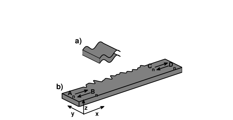
Figure 1: (a) Schematic plot of a out-of-plane mode of an elastic wave propagating in a thin plate. (b) Schematic plot of a two-dimensional rough waveguide that models a thin wire with a rough surface at $y>0$. $A_{n}$, $B_{n}$, $C_{n}$ and $D_{n}$ denote scattering amplitudes. See the text for details.

Heat transport in a solid is a result of unbalanced phonon population. There are mainly two different perspectives in understanding the heat current in nano-materials Mass . One is based on the Kubo formalism, where phonon current is understood as a response to an external temperature field, with the proportionality coefficient expressed as a heat conductivity tensor. Similar to the electron transport case, the conductivity tensor is related to the current-current correlation function. Because the current-current correlation function should be calculated for different phonons and because the phonon number can change (um-klapp process), the Kubo formalism leads to nonlinear equations that are difficult to solve in practice. The other perspective is due to Landauer, where the current can be determined at the surfaces of the sample by applying the correct boundary conditions. In particular, the known solution for outside a sample can be matched at the boundary using a scattering formalism. In this latter framework, from the right bath with temperature $T_{R}$ to the left bath with temperature $T_{L}$, the heat energy flux $J$ is given by

$$J=\frac{1}{2\pi}\sum_{\alpha}\int_{0}^{\infty}dw\ \hbar w(\eta_{R}-\eta_{L})G_{\alpha}(w),$$ (1)

where $w$ is the phonon frequency, $G_{\alpha}$ is the throughput of the mode $\alpha$. Here $\eta_{R,L}$ is the phonon distribution given by $\eta_{i}(w)=1/[\exp(\hbar w/k_{B}T_{i})-1]$, where $T_{i}$ are the temperatures, with indices $i=R,L$. Heat conductance is defined by energy flux per temperature difference, i.e.,

$$\kappa=J/\Delta T\approx\partial J/\partial T,$$ (2)

where for small temperature difference ($T_{R}-T_{L})$, $\kappa$ is approximated by the temperature derivative of the energy flux. After substituting $\eta_{i}(w)$ into Eq. (1) we have,

$$\kappa=\frac{\hbar^{2}}{k_{B}T^{2}}\sum_{\alpha}\frac{1}{2\pi}\int_{0}^{\infty}dwG_{\alpha}(w)\frac{w^{2}\exp(\hbar w/k_{B}T)}{[\exp(\hbar w/k_{B}T)-1]^{2}},$$ (3)

where we have defined the average temperature $T\equiv(T_{L}+T_{R})/2$. In a perfect wire throughput is unity for each open channel, then $\kappa$ in such a perfect case is given by

$$\kappa=\frac{k_{B}^{2}T\pi^{2}}{3\hbar}N,$$ (4)

where $N$ is the total number of open modes. As seen from Eq. (3), the throughput $G_{\alpha}(w)$ is the main quantity that determines the temperature dependence of $\kappa$ in Landauer’s formalism. In the language of a scattering problem, $G_{\alpha}(w)$ is determined by the absolute value squared of certain scattering amplitudes.

To calculate the throughput of elastic waves in a thin wire, we use a thin plate approximation to treat full elastic wave equations. A schematic plot of a two-dimensional rough waveguide modeling a nanowire with surface disorder is shown in Fig. 1(b). Because at low temperatures contribution from any optical modes is exponentially small Luis , we use an elastic theory to describe elastic wave scattering in a relatively long wire. As we show in Fig. 1(b) as an example, we intend to solve a scattering problem in a wire with the width-length ratio set to be 1:100. We scale all the lengths by the wire width, which is taken to be unity.

The elastic wave equation for our model system is given by

$$\frac{\partial^{2}{\bf u}}{\partial t^{2}}=c_{t}^{2}\nabla^{2}{\bf u}+(c_{l}^{2}-c_{t}^{2})\nabla(\nabla\cdot{\bf u}),$$ (5)

where ${\bf u}$ is the displacement vector , $c_{l}$ is the longitudinal phonon velocity and $c_{t}$ is the transverse phonon velocity Graff . For convenience we also scale the velocities by $c_{t}$. That is, in our calculation $c_{t}=1$. In the thin-plate approximation, the gradient in the $z$-direction is assumed to be zero, thus simplifying Eq. (5). Such an approximation decouples the in-plane acoustic modes from the out-of-plane acoustic modes. Assuming that the in-plane and out-of-plane modes behave in a similar fashion, we confine ourselves to the out-of-plane modes only [see Fig. 1(a)]. Technically speaking, implementing the reaction matrix formulation for out-of-plane modes is also simpler than for in-plane modes. The wave equation for out-of-plane modes becomes

$$\frac{1}{c_{t}^{2}}\frac{\partial^{2}u_{z}}{\partial t^{2}}=\frac{\partial^{2}u_{z}}{\partial x^{2}}+\frac{\partial^{2}u_{z}}{\partial y^{2}},$$ (6)

where $u_{z}(x)$ is the displacement in the $z$ direction. The boundary condition for this wave equation will be specified below.

The next step is to calculate the scattering of the elastic waves in a two-dimensional geometry as shown in Fig. 1(b). We will employ a reaction matrix formulation for this scattering problem. The basic idea of a reaction matrix approach is as follows. First, the system is divided into the lead region and the scattering region. Second, the known solution in the lead region is matched at the boundary with the found solution in the scattering region. This matching is implemented by using a basis set satisfying the appropriate boundary condition. In the following section we will show how the reaction matrix can be constructed based on appropriate basis states.

III Scattering throughput in a thin wire with surface disorder

As learned from electron scattering in a rough waveguide akg2 , it can be expected that disorder-induced localization will also play an important role in elastic wave scattering in a thin wire. Furthermore, if the localization length is smaller than the wire length, then the scattering throughput $G_{\alpha}(w)$ is exponentially small; if the localization length is much larger than the wire length, then $G_{\alpha}(w)$ should be close to unity. Because in the low-temperature regime only a few scattering channels contribute to heat transport, it is also important to realize that the localization length might depend strongly on the phonon frequency Murphy . In particular, based on the Born approximation, the electron localization length is inversely proportional to the structure factor (defined below) of the correlation function of the surface disorder evaluated at twice of the scattering electron wavevector Izr ; akg2 . By direct analogy between the Schrödinger equation for electron matter waves and the elastic wave of matter, we can expect that the correlation function of thin-wire surface disorder can also affect strongly the localization length of a scattering elastic wave. Therefore, we are interested in (i) if it is possible to manipulate the frequency dependence of the scattering throughput of elastic waves, and (ii) to what extent different surface disorders might affect the heat conductance.

For completeness we first discuss how to computationally produce a random surface characterized by $y=1+\eta(x)$ [see Fig. 1(b)]. This can be done by dividing a long wire into pieces, shifting each piece up or down randomly, and then connecting each piece smoothly with a cubic spline function akg2 ; prb1 . Randomness of the surface function $\eta$ thus generated can be described by an auto-correlation function $\langle\eta(x)\eta(x^{\prime})\rangle=\sigma^{2}C_{n}(x-x^{\prime})$, where $\sigma$ is the variance of $\eta(x)$. The Fourier transform of this auto correlation function is defined as the structure factor, denoted $\chi(k)$. For disorder close to a white-noise type or for disorder without long-range correction (computationally, we can only divide the wire region into a finite number of pieces, e.g., 100 pieces, hence the surface disorder we generate is at most close to a white-noise type), the structure factor trivially takes a constant value over a broad range of $k$. To generate a more realistic rough thin wire with “colored” or long-range surface disorder, we define another function $\rho(x)$,

$$\rho(x)=\frac{\sin(|a^{r}|x)-\sin(|a^{l}|x)}{|a^{r}|x}$$ (7)

where $a^{l}$ and $a^{r}$ are two introduced parameters. Consider then a new function $\tilde{\eta}(x)$ resulting from a convolution of $\eta(x)$ with $\rho(x)$, i.e., $\tilde{\eta}(x)=\int dx^{\prime}\rho(x^{\prime})\eta(x-x^{\prime})$. It can be easily shown akg2 that due to this convolution, $\chi(k)$ now becomes a “square bump” function, with the bump edges located at $a^{l}$ and $a^{r}$. That is, $\chi(k)$ is zero for $k<a^{l}$ or $k>a^{r}$ and is a constant in between. This convolution method is used below to produce several “bump” functions as an “engineered” surface-disorder structure factor, with different bump widths. Certainly, one may also combine a number of different $\rho(x)$ functions to generate a rather arbitrary structure factor $\chi(k)$.

III.1 Constructing the reaction matrix

The reaction matrix method is a well-known time-independent scattering formalism. As such we need to consider the stationary solutions to the wave equation in Eq. (6). Let us first substitute the ansatz $\exp(-iwt)u_{z}$ into Eq. (6) Graff , yielding

$$\frac{\partial^{2}u_{z}}{\partial x^{2}}+\frac{\partial^{2}u_{z}}{\partial y^{2}}-\frac{w^{2}}{c_{t}^{2}}u_{z}=0,$$ (8)

where $w$ is the phonon frequency. The realistic boundary condition for $u_{z}$ is given by Graff

$$\frac{\partial u_{z}}{\partial y}=0.$$ (9)

A stationary solution to Eq. (8) for a straight channel satisfying the above “zero-stress” boundary condition at $y=0$ and $y=1$ can then be found, namely,

$$\Psi_{n\emph{l}} = \left(A_{n}\frac{e^{ik_{n}x}}{\sqrt{k_{n}}}-B_{n}\frac{e^{-ik_{n}x}}{\sqrt{k_{n}}}\right)\cos(\frac{n\pi y}{{\it d}});$$ (10)

$$\Psi_{n\emph{r}} = \left(C_{n}\frac{e^{ik_{n}x}}{\sqrt{k_{n}}}-D_{n}\frac{e^{-ik_{n}x}}{\sqrt{k_{n}}}\right)\cos(\frac{n\pi y}{{\it d}}),$$ (11)

where $A_{n}$, $B_{n}$, $C_{n}$, and $D_{n}$ are the scattering amplitudes. The wavevector is given by $k_{n}=\sqrt{w^{2}-(n\pi/{\it d})^{2}}$, where $n=0,1,2,\cdots$. Note that when $k_{n}$ takes imaginary values, the solutions are called “evanescent modes”. As mentioned above, in our unit system $d=1$, the wire length is $L=100$, and the phonon frequency $w$ is in terms of the value of the first mode, i.e., $w_{1}=c_{t}\pi/d=\pi$. We also scale temperature by $T_{D}$, where $T_{D}\equiv\hbar w_{1}/k_{B}$. For a thin wire of a width $d=10^{-6}$cm and for an acoustic transverse phonon speed (Silicon) $c_{t}=5.8410^{5}$ cm/sec, we have $T_{D}=14$K.

In a reaction matrix formulation of wave scattering, solutions in Eqs. (10) and (11) can be taken as “free” solutions in the left and right leads that are connected by the wire. To find the relation between the wave amplitudes $A_{n}$, $B_{n}$, $C_{n}$, and $D_{n}$, these two solutions will be matched with that in the wire. Hence, we need to solve the elastic wave equation in Eq. (8), confined by two boundaries defined by $y=1+\tilde{\eta}(x)$ (or $y=1+{\eta}(x)$ for an almost white-noise type surface disorder) and $y=0$ [see Fig. 1(b)]. To that end a set of eigenfunctions of Eq. (8) satisfying the zero-stress boundary condition are needed. In addition, as one main feature of the reaction matrix formulation akg1 ; akg2 , the derivative of the eigenfunctions with respect to the scattering coordinate $x$ should be zero at the lead-wire interface, i.e., at $x=0$ and $x=L$.

To find the eigenfunctions in the scattering region, we employ a coordinate-transformation technique. That is, we consider two new coordinates $x^{\prime}=x$ and $y^{\prime}=y/[1+\tilde{\eta}(x)]$, where $\tilde{\eta}(x)$ is the surface function of the wire. In the $x^{\prime}-y^{\prime}$ coordinate system, the elastic wave equation becomes complicated. However, it is now considered over a straight channel (see Refs. akg1 ; akg2 for details of this coordinate-transformation technique). In the new coordinate system an eigenstate $\phi_{n}$ satisfying the necessary boundary condition can be written as

$$\phi^{i}(x^{\prime},y^{\prime})=\sum_{m,m^{\prime}}\beta_{m,m^{\prime}}^{i}\frac{2}{\sqrt{L(1+\tilde{\eta}(x^{\prime})}}\cos(\frac{m\pi x^{\prime}}{L})\cos(m^{\prime}\pi y^{\prime}),$$ (12)

where $m,m^{\prime}$ are integers, the summation over $m$ and $m^{\prime}$ must be truncated for practical purposes, and $\beta^{i}_{mm^{\prime}}$ are the expansion coefficients to be found numerically.

Once the eigenstates $\phi^{i}(x^{\prime},y^{\prime})$ with eigenfrequencies $\tilde{w}_{i}$ are obtained, we impose the continuity condition at $x=0$ and $x=L$, yielding a reaction matrix,

$$R_{nm}=\sum_{i=1}^{M}\frac{\phi_{n}^{i}(0)\phi_{m}^{i}({\it l})}{w-\tilde{w}_{i}},$$ (13)

where $M$ is the size of the involved basis sets (exact for $M=\infty$), and $\phi_{n}^{i}=\int_{0}^{1}{\phi^{i}\cos(n\pi y)}$ is the overlap of $i$th eigenstate with the $n$th “channel” solution $\cos(n\pi y)$. The index $n,m$ of the reaction matrix $R_{nm}$ denote the scattering channels associated with real wavevectors $k_{n}$ and $k_{m}$. The reaction matrix $R_{nm}$ can then yield the scattering matrix,

$$S=\frac{I-iKR}{I+iKR},$$ (14)

where $I$ is a unit matrix of the same size with $R$, and $K$ is a diagonal matrix with diagonal elements related to the wavevectors $k_{n}$ akg2 ; prb1 . The scattering matrix then relates the incoming wave with the outgoing wave via

$$\left(\begin{array}[]{c}B_{n}\\ C_{n}\end{array}\right)=S\left(\begin{array}[]{c}A_{n}\\ D_{n}\end{array}\right).$$ (15)

Finally, the total scattering throughput is defined as $G\equiv\sum_{\alpha}G_{\alpha}=\sum_{n,m}|S_{n,m}|^{2}$, where the summation is over all open modes. $G$ essentially describes the total transmission of a scattering wave up to a certain given phonon frequency, without taking into account the actual thermal distribution of these phonon modes.

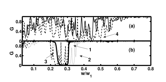
Figure 2: Acoustic phonon transmission in the one-mode regime, as reflected in the dimensionless throughput $G$. (a) Results for two realizations of a waveguide with almost white-noise surface disorder. (b) Results for three different cases of colored surface disorder, with the associated structure factor set as a “square bump” function with three different bump widths. See the text for details.

III.2 Throughput and heat-conductance results

At low temperatures, very few acoustic modes can be populated. Hence it is of interest to examine the scattering throughput in the one-mode regime. This is shown in Fig. 2. Specifically, Fig. 2(a) depicts the results associated with two realizations of a wire with almost white-noise surface disorder. It is seen that when the phonon frequency is small, the throughput $G$ is fluctuating drastically, with its average value far from unity. This indicates that in these two cases the localization length of the elastic wave is comparable to the system size. As the phonon frequency increases, $G$ is seen to be close to unity, suggesting that the localization length is now well beyond the wire length. Figure 2(b) shows what happens if we impose a correlation on the surface disorder, but with the noise variance fixed at $\sigma=0.08$. In particular, the dotted curve (curve 2), the dashed curve (curve 3), and the solid curve (curve 1) are for “engineered” surface functions generated from a convolution of a random surface function $\eta(x)$ with $[\sin(0.7\pi x)-\sin(0.4\pi x)]/(0.7\pi x)$, $[\sin(0.7\pi x)-\sin(0.5\pi x)]/(0.7\pi x)$, and $[\sin(0.6\pi x)-\sin(0.5\pi x)]/(0.6\pi x)$, respectively. It is seen that $G$ develops a clear window for certain phonon frequencies. Despite statistical fluctuations, these throughput windows also show differences in their widths, namely, curve 2 shows the widest window and curve 1 shows the narrowest window. This is consistent with the differences in the bump widths of their associated surface structure factor. We also examined other realizations of random surfaces with the same surface structure factor, confirming that the location of the throughput windows shown in Fig. 2 does not change much. We have also checked that the location of the throughput window quantitatively matches the profile of $\chi(2k)$, the surface structure factor evaluated at twice of the wavevector.

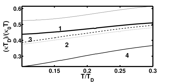
Figure 3: The ratio between heat conductance $\kappa$ and temperature, as a function of temperature, for wire geometries considered in Fig. 2. Thin solid line is for a wire without surface disorder. Line (4) is for a wire with almost white-noise surface disorder. Other lines are for wires with their surface function generated from a convolution of white-noise with some smooth function explicitly given in the text. Here and in all other figures below, the plotted quantity is always dimensionless and $\kappa_{0}\equiv k_{B}w_{1}$.

In Fig. 3 we examine how different properties of the wire disorder might affect the heat conductance $\kappa$ calculated from Eq. (3). To make a better connection with the results in Fig. 2 we examine a temperature regime where thermal excitation only populates at most two channels. First of all, for the case without disorder (upper thin solid curve), the plotted quantity $\kappa/T$ is seen to be roughly a constant for low temperatures. This is somewhat expected because a perfect thin wire is known to show a linear temperature dependence in $\kappa$ at low temperatures. Certainly, as the temperature increases, deviations from the linear behavior emerge due to an increasing contribution from the second populated channel. By contrast, in the presence of surface disorder, the linear temperature dependence of $\kappa$ might not hold from the very beginning of the temperature range shown in Fig. 3 (curves 2,3,4). Interestingly, for different surface disorder, $\kappa/T$ shows quite different behavior. The almost white-noise case (curve 4) deviates most from the case without disorder, with the maximal deviation around a factor of two. These observations suggest that one might achieve some subtle control over the temperature dependence of $\kappa$ in the low-temperature regime by manipulating surface correlations, or say something about the surface correlation by measuring $\kappa$ at different temperatures.

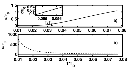
Figure 4: (a) Heat conductance from direct numerical integration (dotted) of Eq. (3) versus the analytical result (solid line) of Eq. (16), for $a=0.2$. As indicated by the inset, the dotted line is on top of the solid line. (b) Same as in (a) but the dashed line is calculated from an expression in Ref. Luis . Note the different scales between panel (a) and panel (b).

To shed more light on how the throughput windows observed in Fig. 2(b) affect the temperature dependence of $\kappa$, let us now consider a model throughput curve that allows for analytical calculations. Consider first two step functions $f_{a}(w)$ and $f_{b}(w)$, namely, $f_{a}(w)=0$ for $w<a$ and $f_{a}(w)=1$ for $w>a$; and $f_{b}(w)=0$ for $w<b$ and $f_{b}(w)=1$ for $w>b$. We denote the heat conductance as $\aleph(a)$ for $G(w)=f_{a}(w)$ and $\aleph(b)$ for $G(w)=f_{b}(w)$, respectively. Assuming that there is only one open mode, we obtain from Eq. (3) that

$$\aleph(a)=k_{B}w_{1}\left(\frac{a^{2}e^{\frac{a}{T}}}{T(e^{\frac{a}{T}}-1)}-2\log\left(e^{a/T}-1\right)a+\frac{2\pi^{2}T}{3}-2T\Re\left[\text{Li}_{2}\left(e^{a/T}\right)\right]\right)$$ (16)

and an analogous expression for $\aleph(b)$, where $Li_{2}$ is the so-called dilog function. Interestingly, at this point we found that the widely cited Ref. Luis does not contain the second term in Eq. (16) and misses a factor of two in the third term. To ensure that our expression is indeed correct we show in Fig. 4(a) that direct numerical integration results based on Eq. (3) are identical with the analytical result of Eq. (16) for $a=0.2$. For the sake of comparison we also show in Fig. 4(b) the associated analytical result of Ref. Luis (dashed line), as compared with the same solid line in Fig. 4(a). Note also that because the function $Li_{2}(z)$ for certain values of $z$ can be explicitly evaluated, it is now possible to predict the exact value of $\aleph(a)$ for certain $e^{a/T}$.

Let us now examine the heat conductance behavior if $G(\omega)$ is a square-well function $G_{sw}(w)$, i.e., it is zero for $a<w<b$ and is unity elsewhere. Because $G_{sw}(w)=f_{b}(w)+1-f_{a}(w)$, one obtains from Eq. (16)

$$\kappa=\frac{k_{B}w_{1}\pi^{2}T}{3}+\aleph(b)-\aleph(a),$$ (17)

where $T$ is already scaled by $T_{D}$. Approximately, for $b>a>>T$, we have

$$\kappa=\frac{k_{B}w_{1}\pi^{2}T}{3}+k_{B}w_{1}\left(\frac{T^{2}(b-a)}{(T-a)(T-b)}\right);$$ (18)

and for $a<b<<T$ we have

$$\kappa=\frac{k_{B}w_{1}\pi^{2}T}{3}+k_{B}w_{1}\left(a-b+2a\log(a)-2b\log(b)+\frac{b^{3}-a^{3}}{36T^{2}}\right).$$ (19)

These two limiting results show that in either case [Eqs. (18) or Eq. (19)], a window in the throughput curve can cause $\kappa/T$ to decrease as compared with what is expected from a linear temperature dependence of $\kappa$.

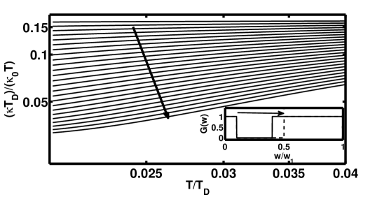
Figure 5: Temperature dependence of $\kappa/T$, for throughput curves modeled by square-well functions. The arrow indicates an increasing width of the square-well function, in steps of 0.08, ranging from 0.0 to 0.4. Note that quantities here are plotted in the logarithmic scale.

From Eq. (17) it is also possible to examine how the width $(b-a)$ of the square well function $G_{sw}(w)$ as a throughput curve affects $\kappa/T$. To that end we show in Fig. 5 a logarithmic plot of $\kappa/T$ versus $T/T_{D}$. The arrow therein indicates an increasing $(b-a)$ in steps of 0.08, which ranges from 0.0 to 0.4. Interestingly, as the throughput window increases its size, $\kappa/T$ decreases. The $\kappa/T$ function is also seen to deviate from a constant function more and more, and a better description of the temperature dependence of $\kappa$ seems to be a power function. We note that this observation is consistent with experimental observations in superconductive materials SYLi . Note also that the analytical result here also explains the general trend seen in our numerical results in Fig. 3. That is, the lowering of $\kappa/T$ curves in Fig. 3 is associated with the widening of the throughput windows shown in Fig. 2(b).

So far we have studied the low-temperature regime where one or two modes are significantly populated. What happens if more phonon modes are populated? To answer this question we show in Fig. 6 the throughput $G(w)$ for up to five modes, for a wire without disorder [case (a)], with almost white-noise surface disorder [case (b)], and with colored surface disorder [cases (c) and (d)]. A number of observations are in order. First, $G(w)$ can be nonzero for phonon frequencies much smaller than $w_{1}$, a feature different from that in electron transport. In the latter case one can only excite the first mode after going beyond the associated cut-off energy. This difference arises from the fact that the Schrödinger equation for electrons and the elastic wave equation for phonons have different boundary conditions. Second, in the presence of surface disorder, the threshold frequency for opening a new channel and hence a drastic increase in $G(w)$ gets higher as compared with the noiseless case. This is analogous to the electron case akg2 , which can be roughly explained via a decrease in the effective wire width. Third, for cases (c) and (d), the dip in $G(w)$ is clear only for the one-mode and two-mode regimes. For higher modes, the throughput dip is no longer clear and is buried by fluctuations in $G(w)$.

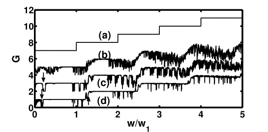
Figure 6: Throughput $G(w)$ versus phonon frequency. Case (a) is for a perfect wire, case (b) is a wire with white-noise surface disorder, and cases (c) and (d) are for two realizations of a wire with colored surface disorder. For a better view cases (c), (b), (a) are shifted upwards by two, four, and six units, respectively. The arrows indicate the dip in the throughput curves. For example, the right arrow for curve (d) indicate a throughput dip in the two-mode regime.

Can those throughput curves in Fig. 6 manifest themselves differently in the heat conductance behavior, when the temperature is high enough to populate many phonon modes? The answer is positive based on the results shown in Fig. 7. In particular, Fig. 7 depicts the temperature-dependence of $\kappa$ for those cases shown in Fig. 6. It is seen that these cases still show quite different behavior even when five phonon modes are significantly populated. Cases (c) and (d) associated with colored surface disorder lie between the curve for a perfect wire and that for a wire with almost white-noise surface disorder. Results in Fig. 7 indicate that for temperatures of the order of $\sim$ 10 K, different surface disorder properties of a thin wire of a width $\sim$ 10 nm may still cause a considerable difference in heat conductance. The results are also plotted on a log-log scale in the inset of Fig. 7. However, we do not see any evident power-law dependence of $\kappa$ versus $T$. This is somewhat expected because the T-dependence of $\kappa$ is quite complicated [see, for example, Eq. (17)]. For the sake of comparison, a perfect wire with twice the width is also shown in Fig. 7 as case (e). In that case the temperature dependence is much stronger. This is anticipated because of the $T^{3}$ scaling of $\kappa$ in bulk materials.

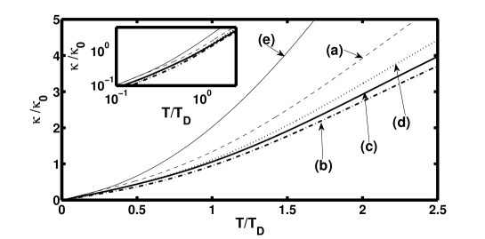
Figure 7: Temperature-dependence of heat conductance for those cases considered in Fig. 6. Case (e) is for a perfect (straight) wire with twice the width, in which the temperature dependence of $\kappa$ is approaching the $T^{3}$ law for bulk materials. Inset shows the same data in a log-log plot.

IV Concluding remarks

In this work we adopted an elastic wave picture of heat transport at sufficiently low temperatures. We presented, for the first time, a reaction matrix treatment of the scattering of elastic waves in thin wires with surface disorder, with realistic zero-stress boundary conditions implemented. We have shown that correlations in the surface disorder can lead to structures in the frequency-dependence of throughput and can hence affect considerably the temperature dependence of heat conductance. Though not done in this study, the heat conductance for a thin wire with an experiment-related surface correlation function can be examined in a straightforward manner. Because our treatment is a natural extension of early electron transport studies, insights gained from studies of electron waveguide transport can now be much relevant to understanding heat transport in thin wires.

Because the boundary condition for in-plane modes of elastic waves is much more difficult to handle for a thin wire of arbitrary shape, here we restrict ourselves to out-of-plane modes only. However, preliminary results show that in-plane modes have similar qualitative behavior as out-of-plane modes.

- (1) L. G. C. Rego and G. Kirczenow, Phys. Rev Lett. 81, 232 (1998).
- (2) K. Schwab, E. A. Henriksen, J. M. Worlock, and M. L. Roukes, Nature (London) 404, 974 (2000).
- (3) A. I. Hochbaum, R. K. Chen, R. D. Delgado, W. J. Liang, E. C. Garnett, M. Najarian, A. Majumdar, and P. D. Yang, Nature, 451 No. 10, 163, (2008).
- (4) S. Y. Li, J.-B. Bonnemaison, A. Payeur, P. Fournier, C. H. Wang, X. H. Chen, and L. Taillefer, Phy. Rev B. 77, 134501 (2008).
- (5) D. Y. Li, Y. Y. Wu, P. Kim, P. D. Yang, and A. Majumdar, Appl. Phys. Lett. 83, 2934 (2003).
- (6) W. X. Li, K. Q. Chen, W. H. Duan, J. Wu, and B. L. Gu, J. Phys.: Condens. Matter 16, 5049 (2004).
- (7) W. X. Li, T. Y. Liu, C. L. Liu, Chin Phys. Lett. 23, 2522 (2006).
- (8) X. F. Wang, M. S. Kushwaha, and P. Vasilopoulos, Phy. Rev B. 65, 035107 (2001).
- (9) H. Y. Zhang, H. J. Li, W. Q. Huang, and S. X. Xie, J. Phys. D: Appl. Phys. 40, 6105 (2007).
- (10) L. M. Tang, L. L. Wang, W. Q. Huang, B. S. Zou, and K. Q. Chen, J. Phys. D: Appl. Phys. 40, 1497 (2007).
- (11) G. B. Akguc and T. H. Seligman, Phys. Rev. B. 74, 245317 (2006).
- (12) M. C. Cross, R. Lifshitz, Phy. Rev B. 64, 085324 (2001).
- (13) R.K. Chen, A. I. Hochbaum, P. Murphy, J. Moore, P.D. Yang, and A. Majumdar, Phy. Rev Lett. 101, 105501 (2008).
- (14) B. A. Glavin, Phy. Rev Lett. 86, 4318 (2001).
- (15) D. H. Santamore and M. C. Cross, Phy. Rev B. 66, 144302 (2002).
- (16) P. G. Murphy and J. E. Moore, Phy. Rev B. 76, 155313 (2007).
- (17) K. Q. Chen and X. H. Wang, and B. Y. Gu, Phy. Rev B. 61, 12075 (2000).
- (18) L. S. Cao, R. W Peng, R. L. Zhang, X. F. Zhang, M. Wang, X. Q. Huang, A. Hu, and S. S. Jiang, Phy. Rev B. 72, 214301 (2005).
- (19) A. Dhar, Phy. Rev. Lett. 86, 5882 (2001).
- (20) Electric Transport in Nanoscale Systems, Massimiliano Di Ventra, Cambridge, 2008.
- (21) Wave Motion in Elastic solids, K. F. Graff, Clarendon Press, Oxford, 1975; Introduction to Elastic Wave Propagation, A Bedford and D. S. Drumheller, John Wiley-Sons, 1994; Theory of Elasticity, 3rd Edition, L.D. Landau and E.M. Lifshitz, Elsevier 1986.
- (22) G. B. Akguc and J.B. Gong, Phys. Rev. B. 78, 115317 (2008).
- (23) F. M. Izrailev and A. A. Krokhin, Phy. Rev. Lett. 82, 4062 (1999).
- (24) G. B. Akguc and J.B. Gong, Phys. Rev. B. 77, 205302 (2008).