Laboratory Experiments, Numerical Simulations, and Astronomical Observations of Deflected Supersonic Jets: Application to HH 110

Abstract

Collimated supersonic flows in laboratory experiments behave in a similar manner to astrophysical jets provided that radiation, viscosity, and thermal conductivity are unimportant in the laboratory jets, and that the experimental and astrophysical jets share similar dimensionless parameters such as the Mach number and the ratio of the density between the jet and the ambient medium. When these conditions apply, laboratory jets provide a means to study their astrophysical counterparts for a variety of initial conditions, arbitrary viewing angles, and different times, attributes especially helpful for interpreting astronomical images where the viewing angle and initial conditions are fixed and the time domain is limited. Experiments are also a powerful way to test numerical fluid codes in a parameter range where the codes must perform well. In this paper we combine images from a series of laboratory experiments of deflected supersonic jets with numerical simulations and new spectral observations of an astrophysical example, the young stellar jet HH 110. The experiments provide key insights into how deflected jets evolve in 3-D, particularly within working surfaces where multiple subsonic shells and filaments form, and along the interface where shocked jet material penetrates into and destroys the obstacle along its path. The experiments also underscore the importance of the viewing angle in determining what an observer will see. The simulations match the experiments so well that we can use the simulated velocity maps to compare the dynamics in the experiment with those implied by the astronomical spectra. The experiments support a model where the observed shock structures in HH 110 form as a result of a pulsed driving source rather than from weak shocks that may arise in the supersonic shear layer between the Mach disk and bow shock of the jet’s working surface.

1 Introduction

Collimated supersonic jets originate from a variety of astronomical sources, including active galactic nuclei (Harris and Krawczynski, 2006), several kinds of interacting binaries (Mirabel & Rodriguez, 1999), young stars (Reipurth & Bally, 2001), and even planetary nebulae (Balick & Frank, 2002). Most current jet research focuses on how accretion disks accelerate and collimate jets, or on understanding the dynamics of the jet as it generates shocks along its beam and in the surrounding medium. Both areas of research have broad implications for astrophysics. Models of accretion disks typically employ magnetized jets to remove the angular momentum of the accreting material. The distribution and transport of the angular momentum in an accretion disk affects its mass accretion rate, mixing, temperature profile, and density structure, and in the case of young stars, also helps to define the characteristics of the protoplanetary disk that remains after accretion ceases. At larger distances from the source, shock waves in jets clear material from the surrounding medium, provide insights into the nature of density and velocity perturbations in the flow, and enable dynamical studies of mixing, turbulence and shear.

Jets from young stars are particularly good testbeds for investigating all aspects of the physics within collimated supersonic flows (see Ray et al., 2007, for a review). Shock velocities within stellar jets are low enough that the gas cools by radiating emission lines rather than by expanding. Relative fluxes of the emission lines determine the density, temperature, and ionization of the postshock gas, while the observed Doppler shifts and emission line profiles define the radial velocities and nonthermal motions within the jet (see Hartigan, 2008, for a review). Moreover, many stellar jets are located relatively close to the Earth, so that one can observe proper motions in the plane of the sky from observations separated by several years (Heathcote & Reipurth, 1992). Combining this information with radial velocity measurements gives the orientation of the flow to the line of sight. Using the Hubble Space Telescope, one can observe morphological changes of knots within jets, and follow how these changes evolve in real time (Hartigan et al., 2001).

Results from these studies show that internal shock waves, driven by velocity variations in the flow, sweep material in jets into a series of dense knots. Typical internal shock velocities are $\sim$ 40 km s^-1, or $\sim$ 20% of the flow speed. In several cases it is easy to identify both the bow shock and the Mach disk from emission line images. Because stellar jets are mostly neutral, strong H$\alpha$ emission occurs at the shock front where neutral H is collisionally excited (Heathcote et al., 1996). Forbidden line radiation occurs in a spatially-extended cooling zone in the postshock material. Temperatures immediately behind the internal shocks can exceed $10^{5}$K, but the gas in the forbidden-line-emitting cooling zone is typically 8000 K.

Young stars show a strong correlation between accretion and outflow, leading to the idea that accretion disks power the outflows (Hartigan et al., 1995; Cabrit, 2007). Most current models use magnetic fields in the disk to launch a fraction of the accreting material from the disk into a collimated magnetized jet (Ferreira et al., 2006). Stellar jets often precess, and there is some evidence that they rotate (Ray et al., 2007), although rotation signatures are difficult to measure because the rotational velocities are typically only a few percent of the flow speeds and precession can mimic rotational signatures (Cerqueira et al., 2006). In all cases proper motion measurements show that jets move radially away from the source. Jets show no dynamical evidence for kink instabilities, and in fact while magnetic fields may dominate in the acceleration regions of jets, they appear to play a minor role in the dynamics at the distances where most jet knots are observed (Hartigan et al., 2007). In the cooling zones behind the shock waves the plasma $\beta$ can drop below unity, so that magnetic fields dominate thermal pressure in those areas. However, the magnetic pressure is small compared with the ram pressure of the jet.

While more unusual than internal working surfaces produced by velocity perturbations, shocks also occur when jets collide with dense obstacles such as a molecular cloud. When the obstacle is smaller than the jet radius, it becomes entrained by the jet, and a reverse bow shock or ‘cloudlet shock’ forms around the obstacle (Schwartz, 1978; Hartigan et al., 2000). Alternatively, when a large obstacle like a molecular cloud deflects the jet, a quasi-stationary deflection shock at the impact point forms, followed by a spray of shocked jet material downstream. The classic example of such a jet is HH 110 (Riera et al., 2003; Lopez et al., 2005).

Though the observations summarized above provide a great deal of information about stellar jets, several important questions remain unanswered. The basic mechanism by which disks load material onto field lines (assuming the MHD disk scenario is correct), and the overall geometry of this wind is unknown, and the roles of reconnection and ambipolar diffusion in heating the jet close to the star are unclear. At larger distances, the magnetic geometry and its importance in shaping the internal working surfaces is poorly-constrained, as are the time scales and spatial scales associated with mixing in supersonic shear layers and working surfaces. The inherently clumpy nature of jets also affects the flow dynamics and observed properties of jets in uncertain ways, and the degree to which fragmentation and turbulence influence the morphologies of jets is unknown.

Developing laboratory analogs of stellar jets could help significantly in addressing the questions above. Observations of a specific astronomical jet are restricted to a small range of times and to a particular observing angle, while laboratory experiments have no such restrictions. In principle, one could explore a wide range of initial collimations, velocity and density structures within the jet, as well as densities, geometries, and magnetic field configurations with laboratory experiments. The experiments also provide a powerful and flexible way to test 3-D numerical fluid codes, and to investigate how real flows develop complex morphologies in 3-D.

The challenge is to design an experiment that is relevant to the astrophysical case of interest. Laboratory experiments differ by 15 $-$ 20 orders of magnitude in size, density and timescale from stellar jets, but because the Euler equations that govern fluid dynamics involve only three variables, time, density, and velocity, the behavior of the fluid is determined primarily by dimensionless numbers such as the Mach number (supersonic or subsonic), Reynolds number (viscous or inertial), and Peclet number (importance of thermal conduction). If the experiments behave as a fluid and have similar dimensionless fluid numbers as those of stellar jets, then the experiments should scale well to the astrophysical case (Ryutov et al., 1999). Other parameters, such as magnetic fields and radiational cooling are more difficult to match, and it is impossible to study the non-LTE excitation physics in the lab because the critical density for collisional deexcitation is not scalable. In any case, the materials are markedly different between the experiments and stellar jets, so it is not possible to study emission line ratios in any meaningful way with current laboratory capabilities. Hence, at present the main utility of laboratory experiments of jets is to clarify how complex supersonic flows evolve with time.

Laboratory work relevant to stellar jets is an emerging area of research, and several papers have appeared recently which address various aspects of supersonic flows in the appropriate regime (see Remington et al., 2006, for a review). Hansen et al. (2007) observed how a strong planar shock wave disrupts a spherical obstacle and tested numerical models of the process, and Loupias et al. (2007) generated a laboratory jet with a Mach number similar to that of a stellar jet. In a different approach, Lebedev et al. (2004) and Ampleford al. (2007) used a conical array of wires at the Magpie facility to drive a magnetized jet, and explored the geometry of the deflection shock formed as a jet impacts a crosswind. Laboratory experiments have also recently studied the physics associated with instabilities along supernova blast waves (Kuranz et al., 2007; Drake et al., 2009), and the dynamics within supernovae explosions (Reighard & Drake, 2007).

In this paper we present the results of a suite of experiments which deflect a supersonic jet from a spherical obstacle, where the dimensionless fluid parameters are similar to those present in stellar jets. In section 2, we describe our experimental design, consider how the experiments scale to astrophysical jets, demonstrate that the experiments are reproducible, and report how the observed flows change as one varies several parameters, including the distance between the axis of the jet and the obstacle, the time delay, the density probed with different backlighters, and the viewing angle. The numerical work is summarized in section 3. Detailed calculations with the 3-D RAGE code reproduce all of the major observed morphologies well. In section 4, we present new high-resolution optical spectra of the shocked wake of the HH 110 protostellar jet, and a new wide-field H₂ image of the region. These observations quantify how the internal dynamics of the gas behave as material flows away from the deflection shock and show how the jet entrains material from the molecular cloud core. Finally, in section 5 we consider how the experiments and the simulations from RAGE provide new insights into the internal dynamics of deflected supersonic jets, especially in the regions of the working surface and at the interface where jet material entrains and accelerates the obstacle.

2 Laser Experiments of Deflected Supersonic Jets

2.1 Experimental Design

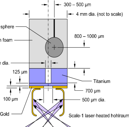
Figure 1: Cross section of the target design for the Omega laser experiments. X-rays produced when the laser impacts the hohlraum accelerate a shock wave into the Ti disk, and a piece of this disk accelerates up the axis (dashed line) to produce a supersonic jet. Subsequent collapse of the evacuated cavity generates a secondary jet along the same direction. The jets move into a cylinder of hydrocarbon foam, and deflect from a polystyrene sphere located at some distance (the impact parameter) from the axis of the cylinder.

Figure 1 shows the experimental assembly we used to collide a supersonic jet into a spherical obstacle. The design consists of a 125 $\mu$m thickness titanium disk in direct contact with a 700 $\mu$m thickness titanium washer with a central, 300 $\mu$m diameter hole. The surface of the disk is heated by the thermal (soft x-ray) radiation from a hohlraum laser target, which itself is heated by 12 beams of the Omega laser at the University of Rochester (Soures et al., 1996). X-ray driven ablation of the surface of the disk creates a near-planar shock within the disk and washer assembly, and the subsequent breakout of this shock from the inner surface of the disk results in the directed outflow of a plug of dense, shock-heated titanium plasma through the cylindrical hole in the washer. This outflow is further collimated by the hole in the washer, and directed into an adjacent block of low-density (0.1 g cm^-3) polymer foam within which it propagates to a distance of $\sim$ 2 mm in $\sim$ 200 ns.

After the primary jet forms, the ablation-driven shock continues to progress through the titanium target assembly and along the sides of the hole in the washer. As the hole collapses inward a secondary jet of material forms by a process analogous to that occurring in a shaped-charge explosive. The secondary jet forms after the primary jet, and propagates into the high-pressure cocoon of material already within the polymer foam. At later times, the shock propagates from the surrounding titanium washer into the foam, and causes the interface between the titanium washer and the hydrocarbon foam to move. A bow shock runs ahead of the jets into the foam. Both jets form as a result of hydrodynamic phenomena alone; there is no significant magnetic field and associated magneto-hydrodynamics, and the temperature of the jet is sufficiently low for thermal-conduction and radiative energy losses to be insignificant. Hence, the hydrodynamic phenomena which determine how the jet forms and evolves are scalable (see Section 2.2) to jets of very different dimensions that evolve over very different timescales.

The experimental assembly described above is identical in many respects to that used in experiments we have reported previously (Foster et al., 2005), but with the following two significant differences (see Rosen et al., 2006; Coker et al., 2007, for further details): (1) in the present case we use indirect (hohlraum) drive, instead of the direct laser drive used in our earlier work; and (2) the foam medium through which the jet propagates contains an obstacle (a ball of CH). The hohlraum drive enables us to obtain greater spatial uniformity of the ablation of the titanium surface, and thereby generates a jet of improved cylindrical symmetry. The (optional) addition of an obstacle in the foam along the path of the jet medium makes it possible to set up, and in a controlled manner test, how the flow behaves when the two-dimensional cylindrical symmetry is broken. A pinhole-apertured, laser-produced-plasma, x-ray backlighting source projects an image of the jet onto radiographic film for later, detailed analysis.

Details of the experimental setup are as follows. A 1600 $\mu$m diameter, 1200 $\mu$m length (internal dimensions) cylindrical gold hohlraum target with a single 1200 $\mu$m diameter laser-entry hole (see also Foster et al., 2002) generates the radiation drive. The experimental package mounts over an 800 $\mu$m diameter hole in the end wall of the hohlraum, immediately opposite the laser entry hole. This axisymmetric configuration enables us to model the assembly at high resolution using two-dimensional radiation hydrocodes during the stages of formation and early-time evolution of the jet; the later stages of three-dimensional hydrodynamics are modeled by linking to a three-dimensional hydrocode, albeit at lower spatial resolution. The hohlraum is heated by 12 beams of the Omega laser with a total energy of 6 kJ in a 1 ns duration, constant power laser pulse of 0.35 $\mu$m wavelength. The resulting peak radiation temperature in the hohlraum measured with a filtered x-ray diode diagnostic (Dante) is 190 $-$ 200 eV (Foster et al., 2002).

The titanium experimental assembly is made of an alloy with 90% titanium, 6% aluminium, and 4% vanadium. The diamond-polished surfaces of the hole and the planar surfaces of the components each have a 0.05 $-$ 0.3 $\mu$m peak-valley, and 0.01 $-$ 0.03 $\mu$m RMS, surface finish. We place a 100 $\mu$m thickness, 500 $\mu$m diameter gold ‘cookie-cutter’ disk between the hohlraum and the titanium disk to control the area of the titanium disk illuminated by x-rays, and to control the time it takes shocks to propagate into the titanium washer. By this means we are able to adjust, to some extent, the relative importance to the overall hydrodynamics of the primary and secondary jets, and the late-time motion of the titanium/foam interface that surround both jets. The medium through which the jets propagate is a 4 mm diameter, 6 mm length cylinder of resorcinol-formaldehyde (C₁₅H₁₂O₄; hereafter RF) foam, of 0.1 g cm^-3 density.

We used RF foam because it has a very small ($<$ 1 $\mu$m) pore size. The obstacle in the foam is a 1 mm diameter, solid polystyrene (1.03 g cm^-3 density) sphere, supported by a small-diameter, silicon-carbide-coated tungsten stalk. The axial position and radial offset (impact parameter) of the sphere within the monomer material is set (approximately) before polymerisation of the foam, but is determined accurately after polymerisation by inspecting each experimental assembly radiographically. Typically, the axial position of the center of the ball, relative to the titanium-to-foam interface is 800 $-$ 1000 $\mu$m, and the impact parameter (perpendicular distance from the axis of the jet to the centre of the ball) is in the range 300 $-$ 500 $\mu$m. We could determine these quantities with an accuracy of approximately $\pm$ 10 $\mu$m, by analyzing pre-shot radiographs of the experimental assembly. The process of target fabrication is to some extent non-repeatable, and necessitates a separate hydrocode simulation of each experimental shot once the target dimensions are known. A sequence of experimental shots, diagnosed at different times, thus measures the hydrodynamic behavior of several very similar (but not strictly identical) target assemblies.

A thin-foil, transition-metal, laser target illuminated with 2 $-$ 5 beams of the Omega laser creates the x-ray point backlighting source we use to diagnose the hydrodynamics. Each beam provides 400 J of energy in a 1 ns duration laser pulse, focused into a 600 $\mu$m diameter spot (spot size determined by use of a random-phase plate). X-ray emission from this laser-produced plasma passes through a laser-machined pinhole of typically 10 $-$ 20 $\mu$m diameter in 50 $\mu$m thickness tantalum foil, and generates a backlighting source of size comparable to the pinhole aperture. He-like resonance-line radiation of the backlighter target material dominates the spectrum of this x-ray backlighting source, and the choice of backlighter targets of typically titanium, iron or zinc results in He-like resonance line radiation of, respectively, 4.75, 6.7 and 9.0 keV.

Radiation from the point x-ray backlighting source creates a point-projection (shadow) image of the experimental assembly on Kodak DEF x-ray film, with approximately 10-times magnification. Temporal resolution is determined by the duration of the x-ray backlighting source (very nearly equal to the laser pulse length). Motion blurring is insignificant for the 1 ns duration backlighting source. The time delay between the laser beams heating the hohlraum target, and the laser beams incident on the x-ray backlighting target is varied from shot to shot to build up a sequence of x-ray images of the jet hydrodynamics.

2.2 Scaling the Experiments to Stellar Jets

The size scales, times, densities and pressures within the Omega experiments differ markedly from those present in stellar jets. For the laboratory results to be meaningful the fluid dynamical variables must scale well, and the experiment should resemble the overall density and velocity structures present in astrophysical jets. We can connect the fluid dynamics of the astrophysical and experimental cases through the Euler equations for a polytropic gas (e.g. Landau & Lifshitz, 1987)

$${{\partial\rho}\over{\partial t}}+\nabla\cdot\left(\rho\bf{v}\right)=0$$ (1)

$$\rho\left({{\partial\bf{v}}\over{\partial t}}+\bf{v}\cdot\bf{\nabla v}\right)+\nabla{\rm P}=0$$ (2)

$${{\partial{\rm P}}\over{\partial t}}+\gamma{\rm P}\nabla\cdot\bf{v}+\bf{v}\cdot\nabla{\rm P}=0,$$ (3)

where $\rho$ is the density, $\bf{v}$ is the velocity, and P is the gas pressure. Ryutov et al. (1999) showed that these equations are invariant to the rescaling

$$r^{\prime}=ar;\ \ \ \rho^{\prime}=b\rho;\ \ \ P^{\prime}=cP$$ (4)

where a, b, and c are constants, provided one also rescales the time as

$$t^{\prime}=a\sqrt{{b\over c}}t.$$ (5)

With this scaling, the velocity transforms as

$$V^{\prime}=\sqrt{{c\over b}}V.$$ (6)

Solutions to the Euler equations will be identical in a dimensionless sense provided equation 6 holds.

Hence, to verify that the experiment scales to the astrophysical case we need to estimate the pressures, temperatures, and velocities in both the experiment and in the HH 110 system. The parameters in the jet differ from those in the working surface where the jet deflects from the obstacle, and from those in the working surface where the bow shock impacts the ambient medium, so we must consider these regions separately. The density and temperature vary throughout stellar jets as material encounters weak shocks, heats, and cools, so we are interested in order of magnitude estimates of these quantites for the scaling estimates. As the discussion below will show, the two working surfaces scale well in our experiment but the jet scales less well.

Consider the parameters in the jet first. Unlike most other jets from young stars, the HH 270 jet that collides with the molecular cloud to produce HH 110 is rather ill-defined, and consists of several faint wisps that resemble weak bow shocks (Choi & Tang, 2006). The electron density and ionization fraction in this part of the flow is poorly-constrained by observations, but an electron density of $10^{3}$ cm^-3 is typical for faint shocked structures of this kind. Taking a typical ionization fraction of 10% we obtain a total density of $10^{4}$ cm^-3, or about $2\times 10^{-20}$ g cm^-3. These values refer to the material in the radiating bow shocks; densities (and temperatures) between the bow shocks are likely to be lower. The temperature where [S II] radiates in the HH 270 bow shocks will be $\sim$ 7000 K. Material in the jet is mostly H, so using the ideal gas law we obtain 1$\times 10^{-8}$ dyne cm^-2 for the pressure.

As shown in Table 1, a $\sim$ $5\times 10^{16}$, b $\sim$ $2\times 10^{-20}$, and c $\sim$ $3\times 10^{-19}$. With this scaling, 200 ns in the laboratory experiments corresponds to $\sim$ 80 years for an HH flow. Bow shocks in HH objects typically move their own diameter in $\sim$ 20 years, so the agreement with the observed timescales of HH objects and the experiment is ideal. However, the jet velocity transforms less well, with 10 km s^-1 in the experiment scaling to $\sim$ 40 km s^-1 in the stellar jet, where the actual velocity is a factor of four higher. This difference arises in part because the stellar jet cools radiatively, lowering the pressure and therefore the value of c. Another way to look at the velocity scaling is to consider the Euler number V/V_E, where V_E = (P/$\rho$)^0.5 is the sound speed for $\gamma$=1. The Euler number in the HH 270 jet is about 20, and for other stellar jets may range up to 40. In the experiment this number is only $\sim$ 6.

The main effect of the difference in Euler numbers is that the experimental jet has a wider opening angle than the stellar jet does. However, both numbers are significantly larger than unity, so both jets are highly supersonic. As we discuss in section 2.3, collapse and subsequent rebound of the washer along the axis of the flow determines to a large extent how the experimental jet is shaped, and has no obvious astrophysical analog. For this reason we will focus our analysis primarily on the leading bow shock and on entrainment of material in the obstacle rather than on the collimation of the jet.

The working surfaces are generally modeled well by the experiment. In these regions the critical parameters are the timescales, which match very well, the Mach numbers in the shocks, and the density contrasts between the jet and the material ahead of the working surface. In stellar jets, the velocity of the bow shock into the preshock medium (equivalently, the velocity of the preshock medium into the bow shock) is similar to that of the jet, $\sim$ 200 km s^-1, because the jet is much denser than the ambient medium. The sound speed in the ambient medium can range from 1 $-$ 10 km s^-1, depending on how much ambient ultraviolet light heats the preshock gas. So the Mach number of the leading bow shock can range from about 20 $-$ 200. In our experiments, the sound speed ahead of the bow shock is low ($\sim$ 0.03 km s^-1), so the Mach number of the leading bow shock in the experiments is also very large, $\sim$ 200. When a stellar jet encounters a stationary obstacle like a molecular cloud, the preshock sound speed is that of the molecular cloud, $\lesssim$ 1 km s^-1, so the Mach number of material entering the shock into the molecular cloud is $\gtrsim$ 200. The Mach number of this shock in the experiments depends on the impact parameter, but is typically $\gtrsim$ 100.

The ratio $\eta$ of the density in the jet to that in the ambient medium to a large extent determines the morphology of the working surface that accelerates the ambient medium. Overdense jets with $\eta$ $>$ 1 act like bullets, and have strong bow shocks and weak Mach disks, while the opposite case of $\eta$ $<$ 1 produces jets that ‘splatter’ from strong Mach disks (sometimes called hot spots) and create large backflowing cocoons (Krause, 2003). Stellar jets are overdense, with $\eta$ $\sim$ 10 while extragalactic jets are underdense with $\eta$ $\lesssim$ $10^{-3}$ (Krause, 2003). In our experiments, $\eta$ ranges from 8 $-$ 1 between 50 ns and 200 ns, respectively, in good agreement with the overdense stellar jet case. For the obstacle, the molecular cloud density increases from at least an order of magnitude less than that of the jet in the periphery of the cloud (essentially the ambient medium density), to $\gtrsim$ 2 orders of magnitude larger than the jet at the center of the core. So the equal densities of the jet and obstacle in the experiment cover a relevant astrophysical regime. The main difference between the experimental and astrophysical cases is the uniform density of the experimental obstacle as compared with the $\sim$ r^-2 density falloff in an isothermal molecular cloud core.

Internal shock waves are by far the most common kind of shock in a stellar jet. Here, velocity perturbations of 30 $-$ 60 km s^-1 produce forward and reverse shock waves within a jet as it flows outward from the source at 150 $-$ 300 km s^-1 (e.g. Hartigan et al., 2001). Gas behind these shock waves cools rapidly to $\sim$ 4000 K by emitting permitted and forbidden line radiation (e.g. Hartigan et al., 1987), and then more slowly thereafter. Typically the temperature falls to $\sim$ 2000 K before the gas encounters another shock front, so the sound speed of the preshock gas is $\sim$ 5 km s^-1. Hence, the internal Mach number is $\sim$ 10 for these shock waves.

Unlike the astrophysical case, our experiments do not produce multiple velocity pulses, and so are less relevant to studying the internal shocks within the beams of stellar jets. However, when jets are deflected obliquely from an obstacle the velocities in the deflected flow can remain supersonic, and may form weaker shocks in the complex working surface area that lies between the leading bow shock and the deflection shock (Mach disk analog) within the jet. Our experiments are very useful for studying the dynamics of this region, and for investigating how a jet penetrates and accelerates an obstacle along its path.

For scaling to hold, several additional conditions must apply. First, dissipation mechanisms such as viscosity and heat conduction must be negligible. Hence, the Reynolds number $Re\sim VL/(\nu_{mat}+\nu_{rad})$ and Peclet number $Pe\sim VL/\chi$, need to be much larger than unity, where $\nu_{mat}$ and $\nu_{rad}$ are kinematic viscosities for matter and radiation, respectively, and $\chi$ is the thermal diffusivity. Using expressions for $\nu_{mat},\nu_{rad}$, and $\chi$ from Ryutov et al. (1999) and Drake et al. (2006), we find thermal conductivity and viscosity are unimportant for both the experimental and astrophysical cases (Table 1).

The Euler equations above implicitly assume that the gas behaves as a polytrope. In reality, stellar jets cool by radiating emission lines from shock-heated regions, and so are neither adiabatic ($\gamma$ = 5/3) nor isothermal ($\gamma$ = 1). Existing numerical simulations provide some insight into how jet morphologies change between the limiting cases of adiabatic and isothermal. In the adiabatic case, material heated by strong shocks cools by expanding, so working surfaces of jets tend to have rounder and more extended bow shocks, while working surfaces collapse into a dense plug for strongly-cooling jets (e.g. Blondin et al., 1990). The effect is less pronounced for weaker oblique shocks like those we are studying here in the wakes of the deflected flows. However, cooling should affect the morphologies of the stronger shocks as described above.

In order to use the Euler equations, the laboratory jet must act as a fluid. Hence, the material mean free path ($\lambda_{mat}\sim v_{th}/\nu_{c}$ where $v_{th}\sim\sqrt{(}k_{B}T/m)$ is the particle thermal velocity and $\nu_{c}$ is the sum of ion and electron collisional frequencies) of the electrons and ions must be short compared with the size of the system ($\tau_{mat}\sim L/\lambda_{mat}\gg 1$). Table 1 shows that this condition is easily satisfied in both stellar jets and the laboratory experiments.

The Euler equations do not include the radiative energy flux, and so we must verify that this number is small compared with the hydrodynamical energy flux. When, as in our experiments, the minimum radiation mean free path $\lambda_{rad}$ from Thomson scattering or thermal bremsstrahlung is short compared to $L$ (i.e., $\tau_{rad}\sim L/\lambda_{rad}\gg 1$), the appropriate dimensionless parameter for determining the importance of radiation is the Boltzmann number Bo# $\sim\rho U^{3}/f_{rad}$, where $U$ is a velocity scale and $f_{rad}$ is the radiative flux. In the Omega experiments, Bo# $>>$ 1, implying that the radiative energy flux is unimportant in the flow dynamics. Radiative fluxes are also negligible in optically thin astrophysical shocks like those in stellar jets. Even in the brightest jets the observed radiative luminosity is $\lesssim$ $10^{-3}$ of the energy of the bulk flow Brugle et al. (1981), so the observations and experiments are consistent with regard to radiative energy flux.

Finally, stellar jets have magnetic fields while our experiments do not. Field strengths within stellar jets are difficult to measure, but could dominate the flow dynamics close to the acceleration region (i.e., V_Alfven $<$ V_flow Hartigan et al., 2007). At the larger distances of interest to these experiments, fields are weaker and act mainly to reduce compression in the postshock regions of radiatively-cooling flows (Morse et al., 1992).

In summary, the experiments are good analogs of jets from young stars. The Mach numbers of the jet relative to the ambient medium and to the obstacle are high in both cases, the density contrasts between the jet and the obstacle are similar, and the scaled times match almost exactly. Both systems behave like fluids, and viscosity, thermal conduction, and radiative fluxes are unimportant to the dynamics in both cases. The main differences are that stellar jets cool radiatively and the experimental jets do not, stellar jets may have magnetic fields that are not present in the experimental jets, and the density profile within the experimental jet is unlikely to have an astrophysical analog.

2.3 Results

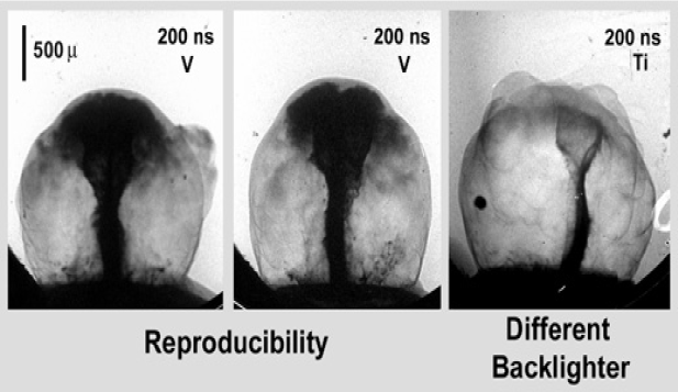
Figure 2: Effect of target fabrication, alignment, and backlighter type on the experiment. Left and center: radiographs of targets without obstacles, taken at 200 ns with a V backlighter. Small differences in the shape of the bow shock and jet are caused by target irregularities. Right: Same as the other images but with a Ti backlighter, which penetrates deeper into the flow.

The complete suite of our experimental radiographs are available on the web (http:$//$ sparky.rice.edu$/\sim$hartigan$/$LLE_shots.html). Because our experiment generates only a single image for each shot, if we wish to investigate how the flow changes with time or compare experiments that have different offsets of the ball from the axis of the jet (we refer to this distance as the ‘impact parameter’ in what follows), we must first quantify the degree to which target fabrication affects the radiographs of the flow. To this end, we obtained several groups of laser shots that had identical backlighters and delay times. One such set appears in Fig. 2, where the overall morphology of the flow and position of the bow shock is reproduced well between the shots, but irregularities appear in the bow shock shape that are specific to each target. In the case of the Ti backlighter image the bow shock resolves into a collection of nearly cospatial shells. The level of difference between the two images at the left of Fig. 2 indicates a typical variation caused by target fabrication and alignment.

We varied the backlighter type, exploring V, Fe, Zn, and Ni. Each backlighter has a different opacity through the material, making it possible to probe the different depths within the structure of the flow at any given time. For example, the Ti backlighter image in Fig. 2 has significantly less opacity than that of the V images. We also tested four different types of foam, normal RF, large-pore RF, TPX (poly-4-methyl-1-pentene), and DVB (divinylbenzene), and found that the neither the foam pore size nor the foam type had any effect on the results.

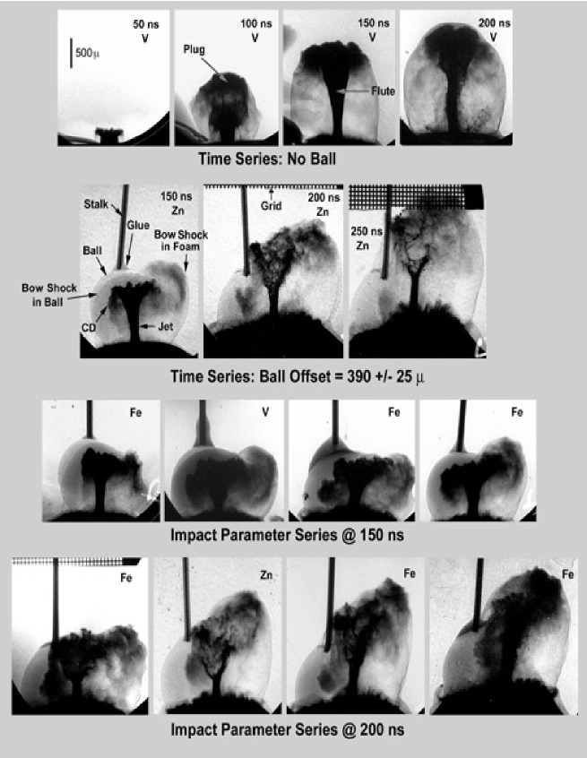
Figure 3: Experimental radiographs of deflected supersonic flows. Top: time series without an obstacle; second row: time series with an obstacle; bottom two rows: increasing the impact parameter (left to right) offset of the ball from the axis of the jet for delay times of 150 ns and 200 ns. The backlighter types (V, Zn, or Fe) are shown. CD denotes the contact discontinuity between the shocked jet and shocked ball material.

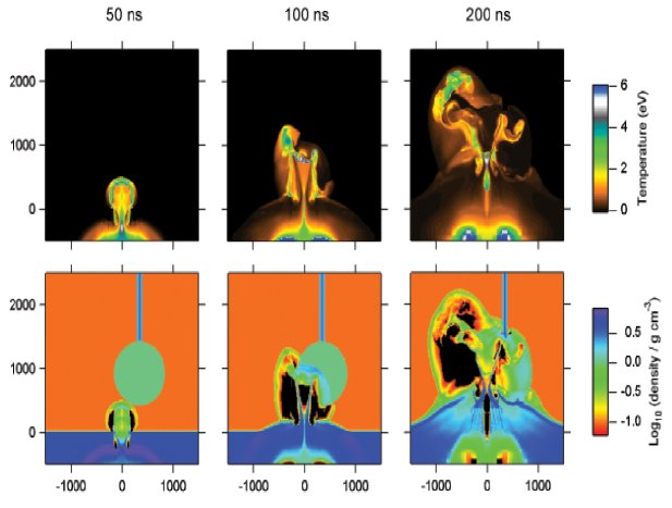
Figure 5: RAGE simulations of the laboratory experiments. The top and bottom rows show the temperature and the density, respectively, at three different times. Scales on the x- and y-axes of the images are in microns.

Fig. 3 summarizes the results from our experiments. The time sequence at the top shows how the jet evolves in a uniform medium without an obstacle. As described in section 2.1, the experiment first accelerates a plug of Ti into the foam, followed by a secondary jet of Ti that originates primarily from the collapse of the washer. At 50 ns, the radiograph shows a flat-topped profile that defines the shape of the plug, and as the plug proceeds into the foam the leading shock becomes bow-shaped. Irregularities in the shape of the bow shock are similar in size and shape to those caused by variations in the manufacture of the target (Fig. 2). By 100 ns the secondary jet has also formed, but it does not become well-collimated until about 200 ns. At 150 ns the end of the jet has a flute-shape, with a less-dense interior (see also Fig. 5, below). This shape is not a particularly good analog for a stellar jet, so we place less emphasis on this area in our analysis.

The second row in Fig. 3 illustrates the principal shock structures that form when the jet encounters a sperical obstacle (labeled ‘Ball’ in the Figure) along its path. In general we expect two shocks to form when a continuous supersonic jet impacts ambient material $-$ a forward bow shock that accelerates the ambient medium, and a reverse shock, sometimes called a Mach disk, that decelerates the jet. The area between the forward and reverse shocks is known as the working surface, and within the working surface there is a boundary known as the contact discontinuity which separates shocked jet material from shocked ambient (or shocked ball) material.

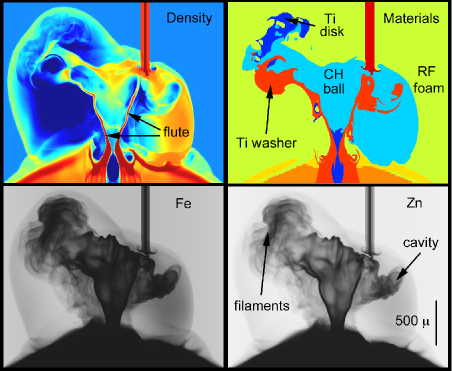
Figure 4: RAGE simulations of the deflected flow at 200 ns with an impact parameter of 350 $\mu$m. Top Left: a slice through the center of the ball showing density (see also Fig. 5). Top Right: composition of the flow. Dark blue denotes material that originated in the Ti disk and was accelerated as the plug, orange represents material from the Ti washer that emerged as the secondary jet. Other materials are the CH ball (light blue), RF foam (yellow-green), and stalk (red). Bottom: simulated radiographs using an Fe and a Zn backlighter. The filamentary structure of the working surface and the cavity driven into the ball by the jet are discussed in the text.

The two forward bow shocks, one into the ball and the other from the deflected jet into the foam, are clearly visible in the radiographs. However, the Mach disks for these bow shocks are more difficult to see in Fig. 3. At 150 ns the Ti plug is the primary driver of the deflected bow shock, and the RAGE simulations discussed below show that the shocked plug is located near the head of the bow shock at this time (Fig. 4). Fig. 5 shows that a disk-shaped area of high temperature material exists in the shocked plug and at the end of the flute, and it is tempting to associate these areas of hot gas with the Mach disk. The situation is complicated by the fact that the plug jet is impulsive, so one would expect the Mach disk to disappear once material in the plug has passed through it, though the temperature will remain elevated in this area.

The last two rows of images in Fig. 3 depict two sequences of radiographs taken at common times after the deposition of the laser pulse, but with impact parameters that increase from left to right. As expected, the jet burrows into the ball more when the impact parameter is smaller, and is deflected more when the impact parameter is larger. In all cases the forward bow shock into the ball is quite smooth, with no evidence for any fluid dynamical instabilities. In contrast, the contact discontinuity between the shocked jet and shocked ball material is highly structured. As we discuss further in section 5, the irregularity of the contact discontinuity plays a major role in breaking up the ball. Images obtained with the Zn backlighter are best for revealing the morphology of the secondary jet, which at late times appears to fragment into a complex filamentary structure in the region of the flute.

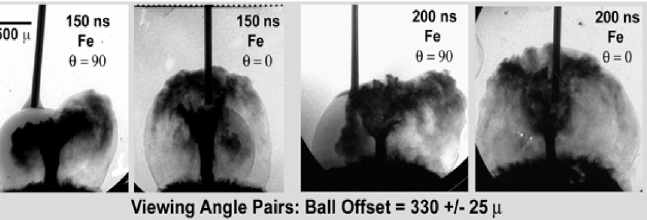
Figure 6: Radiographs of a pair of nearly identical targets imaged with the same backlighter and delay time with orthogonal orientations at 150 ns (left) and 200 ns (right). The ball is clearly visible through the jet in the symmetrical view ($\theta$ = 0) at 150 ns.

The ability to observe a flow from an arbitrary viewing angle is an attractive feature of the laboratory experiments that is not available to astrophysicists who study stellar jets. Fig. 6 shows two pairs of identical laser shots, one with a 150 ns time delay the other with a 200 ns delay, where the viewing angle changed by 90 degrees within each pair. The outline of the ball is clearly visible through the deflected jet in the symmetrical view ($\theta$=0) at 150 ns. Discerning the true nature of the deflected flow is much more difficult in the symmetrical view, where the radiograph resembles a single, less-collimated bow shock.

3 Numerical Simulations of the Laboratory Experiments

The design of these experiments and their post-shot analysis was done with the RAGE (Radiation Adaptive Grid Eulerian) simulation code. We have also adapted the astrophysical MHD code AstroBEAR to model laser experiments by including a laser drive and real equation of state for different materials, but we summarize the results of this work elsewhere (Carver et al., 2009).

3.1 RAGE Simulations

RAGE is a multi-dimensional, multi-material Eulerian radiation-hydrodynamics code developed by Los Alamos National Laboratory and Science Applications International (SAIC) (Gittings, 2008). RAGE uses a continuous (in space and time) adaptive-mesh-refinement (CAMR) algorithm to follow interfaces and shocks, and gradients of physical quantities such as material densities and temperatures. At each cycle, the code automatically determines whether to subdivide or recombine Eulerian cells. The user also has the option to de-zone (that is, reduce the resolution of the mesh) as a function of time, space, and material. Adjacent square cells may differ by only one level of resolution, that is, by a factor of 2 in cell size. The code has several interface-steepening options and easily follows contact discontinuities with fine zoning at the material interfaces. This CAMR method speeds calculations by as much as two orders of magnitude over straight Eulerian methods. RAGE uses a second-order-accurate Godunov hydrodynamics scheme similar to the Eulerian scheme of Colella (1985). Mixed cells are assumed to be in pressure and temperature equilibrium, with separate material and radiation temperatures. The radiation-transfer equation is solved in the grey, flux-limited-diffusion approximation.

Given the placement of the ball with respect to the symmetry axis of the undeflected jet, these experiments are inherently three-dimensional. However, before the jet impacts the ball, the hohlraum and the jet are two-dimensional. This allows us to perform highly resolved, two-dimensional simulations in cylindrically-symmetric geometry to best capture the ablation of the titanium, the acceleration of the titanium plug through the vacuum free-run region in the washer, the collapse of the titanium hole onto the symmetry axis, and the subsequent jet formation.

The two-dimensional simulations are initialized by imposing the measured radiation-drive temperature in a region that is inside the hohlraum. To save computer time, we have determined that it is sufficient to eliminate the hohlraum and just use the measured temperature profile as the source of energy that creates the ablation pressure to drive the jet.

Neglecting asymmetries that arise from initial perturbations and unintentional misalignment of the hohlraum with the vacuum free-run region (the hole in the washer), the early-time experimental data show that the jet remains cylindrically symmetric until at least 50 ns. At approximately this time we link the two-dimensional, cylindrically-symmetric simulation into three dimensions and add the 1 mm diameter ball at the different impact parameters. While the two-dimensional simulations are run with a resolution of 1.5 $\mu$m to capture the radiation ablation of the titanium correctly, the three-dimensional simulations are typically run at lower resolution, especially during the design of the experiments.

Fig. 4 shows the model density, composition, and expected radiograph for a deflected jet at 200 ns. Material labeled as blue (Ti plug) comes from the Ti disk, while orange (Ti sleeve) originates in the Ti washer and constitutes most of the secondary jet. The flute-shape of the secondary jet is clear in this figure. The areas of greatest interest are the region where the jet is creating a cavity in the ball, because this shows how jets destroy obstacles and entrain material, and the region of filaments in the working surface of the leading bow shock, because these filaments could in principle propagate downstream as weak shocks like those seen in HH 110.

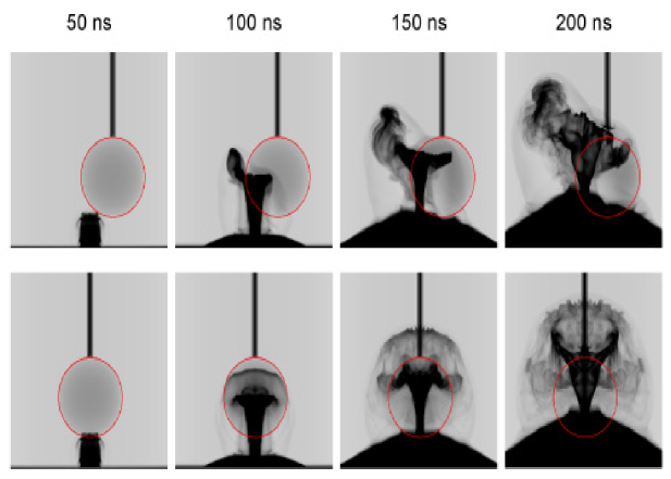
Figure 7: Same simulation as in Fig. 5 but showing predicted radiographs. The location of the ball is marked with a red circle. Top row: asymmetrical view perpendicular to the plane defined by the axis of the jet and the center of the ball. Bottom row: symmetrical view, oriented 90 degrees from the asymmetrical view.

The processes of jet formation and propagation are illustrated in Fig. 5, which show ‘snapshots’ of the temperature and density distribution within the jet taken from a RAGE hydrocode simulation (single choice of axial position and impact parameter for the polystyrene sphere) at different times. The primary (plug) and secondary (‘shaped-charge’ hole collapse) jets are identified in Fig. 5, as well as the late-time motion at the titanium-to-foam interface that results in the formation of an opaque pedestal-like feature at the base of the jet in the synthetic radiographs. All these features are clearly discernible in the experimental data. Fig. 7 shows post-processed, zinc-backlit (9 keV x-ray backlighter energy) radiographic images from two perpendicular views that represent the time evolution of the jet, and how it subsequently deflects from the ball, in the RAGE simulation.

3.2 Data Analysis and Comparisons with RAGE Simulations

The experimental data recording the jet hydrodynamics are in the form of radiographic images recorded on x-ray-sensitive film. Fig. 3 shows a composite of experimental radiographs from several laser shots, to illustrate the formation and deflection of the jets, in a series of shots where the position and impact parameter of the polystyrene sphere inevitably vary somewhat from shot to shot. We digitized the film data with a Perkin-Elmer PDS scanning microdensitometer and converted the film density to exposure using calibration data for the Kodak DEF film that recorded the images (Henke et al., 1986). Ideally, the pinhole-apertured x-ray backlighting source would provide spatially uniform illumination of the experimental assembly, although in practice this is not the case because of laser intensity variations at the backlighting target and vignetting resulting from the specific size and shape of the pinhole aperture. Regions of the image resulting from x-ray transmission through the undisturbed foam (that is, outside the jet-driven bow shock) provide a means to determine the uniformity of backlighting intensity, after we allow for the known x-ray attenuation resulting from the undisturbed foam. Starting from this measured intensity distribution we use a polynomial fitting procedure to infer the unattenuated backlighter intensity that underlies the image of the jet and bow shock. We divide the backlit image data by the inferred (unattenuated) backlighter intensity to obtain a map of x-ray transmission through the experiment. We compare this x-ray transmission data with post-processed hydrocode calculations that simulate the experimental radiographs. Because the absolute variation of backlighter intensity across the image is small (typically, 10 $-$ 20% across the entire image), the polynomial fitting procedure enables the absolute x-ray transmission to be inferred with second-order accuracy.

We use three principal metrics for comparing the experimental radiographs with synthetic x-ray images obtained by post-processing of our hydrocode simulations. These are: (1) the large-scale hydrodynamic motion (determined by comparison of the positions of the bow shock in experiment and simulation); (2) the spatial distribution of mass of the titanium jet material (obtained from the spatial integral of optical depth throughout the image, or from sub-regions of the image); and (3) the small-scale structure in the deflected jet (quantified by the two-dimensional discrete Fourier transform of sub-regions of the image, and its corresponding power spectral density function of spatial frequency).

In making comparison of the experimental with hydrocode simulation, two specific points of detail require attention: (i) each laser-target assembly has its own specific location of the polystyrene sphere within the polymer foam cylinder (because of target-to-target variations arising in fabrication), and (ii) the angular orientation of the polymer-foam cylinder attached to the laser-heated hohlraum target determines the x-ray backlighting line of sight, relative to the plane in which the polystyrene sphere is displaced from the axis of the jet. Ideally all laser targets would be identical, and all backlit images would be recorded orthogonal to the axis of the target, and either in the plane of radial displacement of the polystyrene sphere or orthogonal to that plane.

The geometry of the target chamber of the Omega laser facility determines the possibilities for backlighting orthogonal to the axis of the experimental assembly, and is well-characterized. However, to model a specific experiment fully, we must run three-dimensional hydrocode simulations specific to that experiment which include target-to-target differences of the fabrication assembly, followed by post-processing specific to the backlighter line of sight used in each experiment (which may differ by up to 10 degrees from the two preferred directions dictated by the symmetry of the experiment). The three-dimensional hydrocode simulations are expensive in their use of computing time and resources, and we therefore make detailed comparison of the experimental data with simulation for only a small number of representative cases.

3.2.1 Large-Scale Hydrodynamics and Bow Shock Position

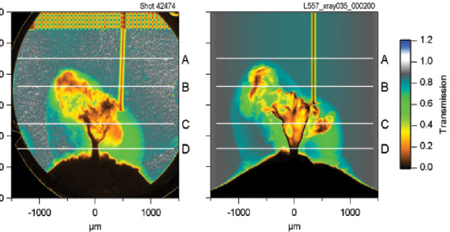
Figure 8: Observed (left) and RAGE simulation (right) of a radiograph image of a deflected supersonic jet. The horizontal lines marked A, B, C, and D mark locations used for further analysis (cf. Figs. 10 and 11).

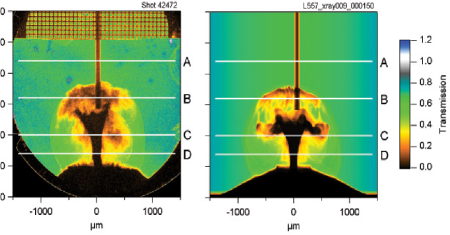
Figure 9: Same as in Fig. 8 but for a symmetrical view.

Figs. 8 and 9 compare images of the deflected jet at 200 ns after the onset of radiation drive to the experimental assembly, and for backlighting lines of sight orthogonal to the plane of jet deflection (Fig. 8) and within the plane of jet deflection (Fig. 9). In each case, the data are compared with post-processed simulations from the RAGE hydrocode. The x-ray backlighting source was the 9.0 keV resonance line of He-like zinc (Fig. 8) or the 6.7 keV line radiation of He-like iron (Fig. 9). In each case, we corrected for spatial variations of incident backlighter intensity (as described above) and the images are therefore maps of absolute backlighter transmission through the experiment. The spatial resolution of both experiments was 15 $\mu$m. The bow shock in the hydrocarbon foam ahead of the jet is clearly visible, as is the late-time hydrodynamic behavior of the primary (outflow) jet (the mushroom-like feature lying off axis, resulting from deflection of the jet) and the secondary (hole-collapse) jet (the dense, near-axis stem apparently penetrating the initial position of the polystyrene sphere). Also evident in the radiographs is the mound-shaped pedestal that arises from motion of the titanium-to-foam interface following shock transit across this interface at late time.

In the case of each experiment (the two images were obtained from different experimental shots) the radial offset of the center of the sphere from the axis (impact parameter) was close to 350 $\mu$m , and the axial position of the center of the sphere was close to 920 $\mu$m . A single RAGE simulation is shown for purposes of comparison, in which the impact parameter was 350 $\mu$m, and the axial position for the sphere 915 $\mu$m. The spatial resolution of this simulation was 3.1 $\mu$m.

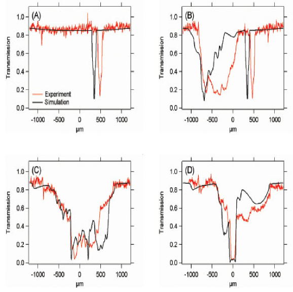
Figure 10: Comparisons between the experiment and the simulation along the lines marked in Fig. 8.

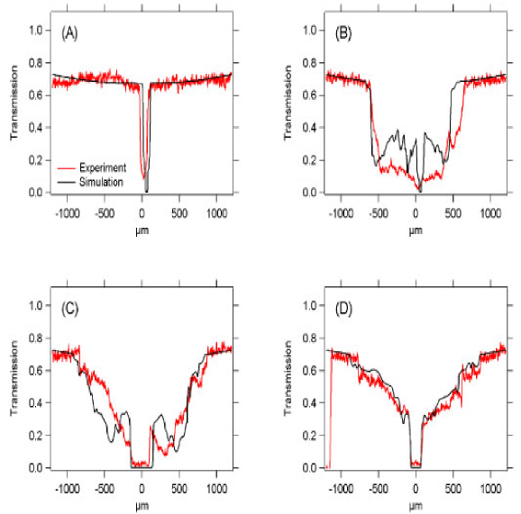
Figure 11: Same as Fig. 10 but for the symmetrical view shown in Fig. 9.

We make quantitative comparisons of experiment and simulation by comparison of lineouts of x-ray transmission in Fig. 10 and Fig. 11. The simulation reproduces the large-scale hydrodynamics of the experiment (bow-shock position, formation of the deflected jet, motion of the pedestal and the creation of a Mach-stem-like feature where it meets the bow shock). However, the simulation does less well with other features of the hydrodynamics, including the “clumpiness” of the deflected jet material and its proximity to the bow shock running ahead of the deflected jet, and the small-scale structure at the interface of the titanium washer and foam (apparently at the surface of the pedestal feature).

The finely-resolved simulations capture more fine-scale structure $-$ the jet does indeed break up into structure similar to that seen in the experiment with simulations at 1 $\mu$m spatial resolution, although at a somewhat later time than observed experimentally. These small-scale structures tend to have larger local Mach numbers and are therefore closer to the bow shock. The filigree structure at the pedestal probably arises from Richtmyer-Meshkov growth of small-scale machining or polishing marks on the surface of the titanium washer, following shock transit across this interface. There are also multiple shock interactions that form Mach stems which are not captured by these simulations owing to the reduced computational resolution in the pedestal area.

3.2.2 Spatial Distribution of Mass

To proceed further with quantitative comparison with simulation, we consider the spatial distribution of mass of the materials present in the experiment. At each point in the experimental and synthetic images, the optical depth at the photon energy of the backlighter radiation is given by

$$\tau=\kappa_{1}\sigma_{1}+\kappa_{2}\sigma_{2}+\kappa_{3}\sigma_{3}$$ (7)

where $\tau$ and $\sigma$ are the opacity and areal density (integral of density along the line of sight) and subscripts distinguish the titanium jet (1), the hydrocarbon foam (2) and the polystyrene sphere (3) materials, respectively. The opacity of the titanium jet is significantly greater than that of either the RF foam or the polystyrene sphere, and their temperatures are sufficiently low for the opacity of these materials to be essentially constant throughout the volume of the experiment. For example, at 9 keV (the photon energy of the zinc backlighting source) the opacities of titanium, RF foam and polystyrene are, respectively, 150, 4.12 and 2.83 cm²g^-1.

We divide the experimentally measured and simulated images, arbitrarily, into 500 $\mu$m square regions, and for each region we calculate the mean optical depth $\bar{\tau}$ using $\tau$ = $-$ln(I/I_∘), and

$$\bar{\tau}={{\int\tau dA}\over{\int dA}}$$ (8)

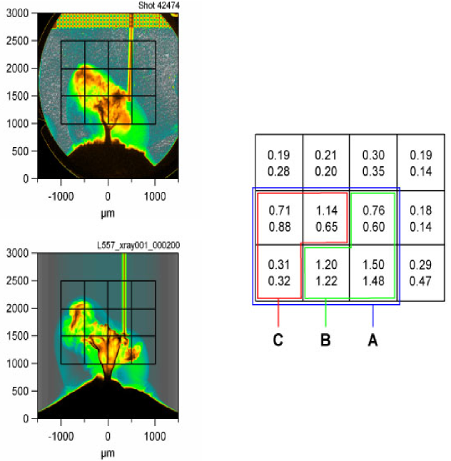
Figure 12: Regions defined for more detailed analysis for the observed radiograph (top) and the RAGE simulation (bottom) as discussed in the text. The top and bottom numbers in each sqaure are the optical depths in the experiment, and simulation, respectively.

where I/I_∘ is the measured (or simulated) x-ray transmission, dA is the pixel area, and the integration extends over the area of each specific region of the image. A comparison of mean optical depth defined in this way, for both experiment and simulation, appears in Fig. 12. The grouping together of adjacent, square regions of the image enables the mean to be calculated for rather larger areas encompassing all of, or the majority of, the mass of the deflected jet. In particular, we consider two larger areas of the images shown in Fig. 12: the rectangular region composed of six adjacent 500 $\mu$m squares and labeled A, and the L-shaped region composed of three adjacent 500 $\mu$m squares and labeled B. These encompass essentially all of the mass of the jet that has interacted with the polystyrene sphere (region A), and all except the mass of the primary jet deflected by the sphere (in the case of the L-shaped region B).

In each case, the simulation reproduces the experimentally measured optical depth to $\sim$ 10%: for the rectangular region A, mean optical depths are 0.94 for the experiment and 0.86 for the simulation; for the L-shaped region B, mean optical depths are 1.15 for the experiment and 1.10 for the simulation. The greatest difference between experiment and the simulation arises in the magnitude and distribution of mass of the primary (outflow) jet deflected by the obstacle. Material from this primary jet resides mainly in a further L-shaped region, labeled C in Fig. 12. Although the mean optical depths for region C differ by only 15% (0.72 in the case of experiment, 0.62 in the case of simulation), the distribution of mass shows significant variation (mean optical depths of 1.14 and 0.65 in the case of the 500 $\mu$m square region where the difference is most evident).

Fig. 12 shows that the RF foam makes only a relatively small contribution to the measured optical depth, but we may assess the magnitude of this contribution simply by setting the opacity of the other components of the experiment (titanium jet and polystyrene sphere) to zero in the post-processing of the hydrocode simulation. We conclude that for the various 500 $\mu$m square regions of the images shown in Fig. 12, the optical depth of the foam lies in the range 0.10 $-$ 0.17 (this variation arises because of chord-length effects, and because density variations of the foam at the bow shock and within the cocoon). Hence, RF foam contributes a negligible optical depth in these experiments.

3.2.3 Discrete Fourier Transform and Power Spectral Density

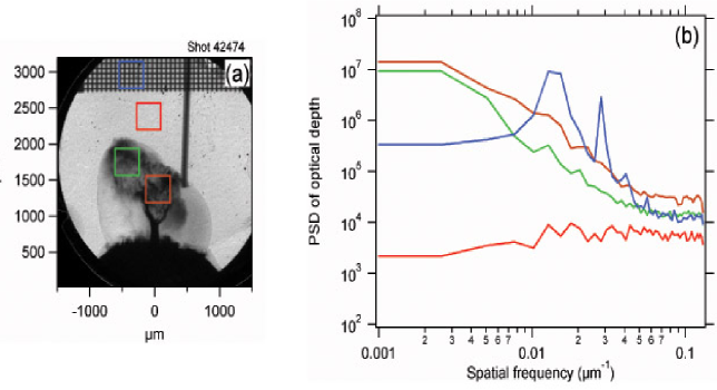
Figure 13: Power spectra of discrete Fourier transforms of four regions in a radiograph image of a deflected jet. The color of the power spectrum curve corresponds to the color of the box marked in the image. The periodic structure of the mesh used to define the spatial scale appears as series of peaks in the blue spectrum.

To compare the experimental data with the small-scale structure of the jet in the simulations, we use the two-dimensional discrete Fourier transform (DFT) of optical depth. Starting from the experimental (or simulated) images of the experiment, we obtain maps of optical depth ($\tau$ = -ln(I/I_∘)) and use the fast Fourier transform algorithm to obtain the DFT of selected regions of the experimental (or simulated) data and then proceed to calculate the power spectral density (PSD). Fig. 13 shows an image of the deflected jet within which we have identified two separate regions (green and dark red boxes), as well as an area of undisturbed hydrocarbon foam (bright red box), and part of the fiducial grid attached to the surface of the foam (blue box). For each region, we show the PSD of optical depth. We define the PSD as the sum of amplitude-squared of all Fourier components whose spatial frequency lies in the range k $-$ k + dk, where k = (k${}_{x}^{2}$ + k${}_{y}^{2}$)^0.5 and k_x and k_y are orthogonal spatial frequency components of the two-dimensional DFT.

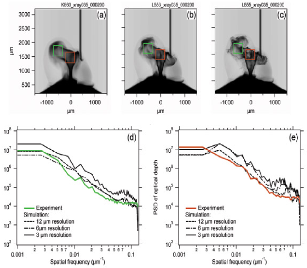
Figure 14: Same as Fig. 13 but for RAGE simulations at 12 $\mu$m, 6 $\mu$m, and 3 $\mu$m resolution (panels a, b, and c, respectively). Panel (d) shows the power spectrum in the deflected wake, while panel (e) shows a similar spectrum near the axis of the jet (green and red boxes, respectively). The colored curves in panels (d) and (e) show the corresponding experimental results.

Fig. 13 clearly shows the fundamental spatial frequency of the grid and its harmonics, the flat spectrum of white noise of the backlighter transmission through the undisturbed foam, and a spectrum arising from the clumpy, perhaps near turbulent, structure arising within the deflected titanium jet. Fig. 14 shows an analogous PSD analysis, for three different RAGE simulations of the experiment. Our approach is the same for the simulation as it is for the experimental data: we obtain a map of optical depth from the simulated radiograph and then the PSD of regions whose size and position is identical to those chosen in analysis of the experimental data. In the case of Fig. 14, we show the result of RAGE simulations for three different levels of AMR calculational resolution: 12.5, 6.25, and 3.125 $\mu$m. Although the calculational resolution (dimension of the smallest Eulerian cell) differs in these three cases, we first obtain (by interpolating the post-processed data) a simulated radiograph with the same spatial resolution as the experimental data before proceeding to calculate the PSD. This procedure enables us to avoid any potential uncertainty of the scaling of PSD amplitude and frequency spacing when comparing with the experimental data.

4 Astronomical Observations and Numerical Models of the Internal Dynamics within the Deflected Jet HH 110

4.1 Spectral Maps of HH 110

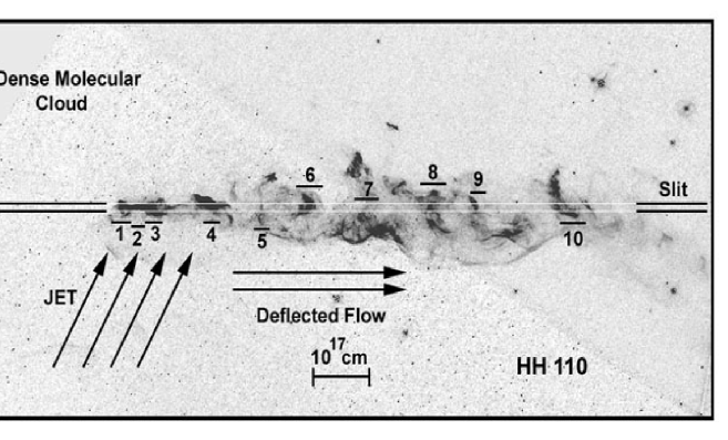
Figure 15: Archival HST emission line image of the HH 110 jet taken through the F658N filter of ACS (P.I. Reipurth). The jet deflects from the molecular cloud as indicated. The slit position used for the spectral observations is shown, and the numbers mark the ten regions used to extract line profiles. The spatial scale assumes a distance of 450 pc.

We observed HH 110 on 9 Jan 2008 UT with the echelle spectrograph on the 4-m Mayall telescope at Kitt-Peak National Observatory in order to quantify the dynamics present in a shocked, deflected astrophysical jet. The 79-63 grating and 226-1 cross disperser combined with the T2KB CCD and 1.5 arcsecond slit gave a spectral resolution of 3.0 pixels, or 11.1 km s^-1 as measured from the FWHM of night sky emission lines. The CCD, binned by two along the spatial direction, produced a plate scale of 0.52 arcseconds per pixel. The position angle of the slit was 13 degrees, and the length of the slit was limited by vignetting to be about 140 arcseconds. Seeing was 1.3 arcseconds, and skies were stable with light cirrus. A plot of the slit position superposed on an archival HST image of HH 110 appears in Fig. 15.

We employed an unusual mode of observation, long slit but with a wide order separating filter (GG 435). This setup causes orders to overlap at different spatial positions along the slit, but in the case of HH 110 there is no ambiguity because no continuum sources are present. The advantage of this setup is that one can obtain position-velocity diagrams simultaneously for all the bright emission lines, including [S II] 6716, [S II] 6731, [N II] 6583, [N II] 6548, and H$\alpha$. The [O I] 6300 and 6363 lines were also present, but the signal-to-noise of these faint lines was too low to warrant any profile analysis. Distortion in the spectrograph optics causes each emission line to be imaged in a curved arc whose shape varies between orders. Fortunately, there is strong background line emission in each of the emission lines from the HH 110 molecular cloud, and we used this emission to correct for distortion and to define zero radial velocity for the object. A third degree polynomial matched the distortion of the night sky emission lines within an rms of about 0.2 pixels (0.74 km s^-1).

It is important to remove night sky emission lines as well as the background emission lines from the molecular cloud, as these lines contaminate multiple orders in our instrumental setup. To this end, we imaged blank sky near HH 110 frequently and subtracted this component from the object spectra after aligning the night sky emission between the object and sky frames to account for flexure in the spectrograph. Cosmic rays and hot pixels were removed using a routine described by Hartigan et al. (2004), and flatfielding, bias correction, and trimming were accomplished using standard IRAF tasks.

Alignment of individual exposures was accomplished in two ways. First, we compared the position of a star relative to the slit that was captured from the guide camera, whose plate scale of 0.16 arcseconds per pixel we determined by measuring the length of the slit image when a decker of known size truncated the slit. More precise positioning in the direction along the slit is possible by extracting the spatial H$\alpha$ trace and performing a spatial cross correlation between frames. The uncertainty in the positional measurements from the guide camera image inferred from the secondary corrections required by the cross-correlations is about 1.0 arcseconds.

To align and compare different emission lines we must also register the position-velocity diagrams to account for the spatial positions of the orders and for the tilt of the spectrum across the CCD within each order, but this is easy to do with a continuum lamp exposure through a small decker to define the spectral trace. The guide camera images indicate, and the spectra confirm, that the last three object exposures drifted by 1.5 arcseconds relative to the position shown in Fig. 15, so these were not used in the final analysis. In all, the total exposure time for the spectra is 140 minutes. There were no differences between the [S II] 6716 and [S II] 6731 position-velocity diagrams, so we combined these to produce a single [S II] spectrum. The [N II] 6548 line is fainter by a factor of three than the companion line [N II] 6583, and the fainter line is also contaminated by faint residuals from a bright night sky emission line from an adjacent order, so we simply use the 6583 line for the [N II] line profiles.

4.2 Internal Dynamics of HH 110

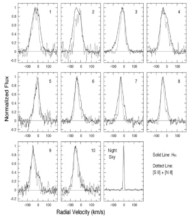
Figure 17: Emission line profiles in HH 110. Solid and dotted lines denote the emission line profiles of H$\alpha$ and [S II]+[N II], respectively, for each of the ten regions along the slit marked in Fig. 15. The night sky profile shows the instrumental resolution. The jet is resolved everywhere, and is somewhat broader in H$\alpha$ than it is in the forbidden lines. The radial velocity becomes more negative as the jet flows downstream from the impact point.

The image in Fig. 15 divides the position-velocity diagram into ten distinct emitting regions along the slit. Spectra for each of these positions appear in Fig. 17 for H$\alpha$ and for the sum of [N II] + [S II]. All regions have well-resolved emission line profiles in H$\alpha$, [N II], and in [S II]. Only object 9 showed any difference between the [S II] and [N II] profiles, with [N II] blueshifted by 12 km s^-1 relative to [S II].

In low-excitation shocks like HH 110, the forbidden line emission peaks when the gas temperature is $\sim$ 8000 K (Hartigan et al., 1995), which corresponds to a spread in radial velocity owing to thermal motions of HWHM = ((2ln2)kT/m)^0.5, or 2.6 km s^-1 for N, and 1.7 km s^-1 for S. These thermal line widths will be unresolved with the Kitt-Peak observations, which have a spectral resolution of 11 km s^-1. Therefore, the observed widths of the forbidden lines measure nonthermal line broadening in the jet. This line broadening most likely arises from nonplanar shock geometry or clumpy morphologies on small scales, as the HST images show structure down to at least a tenth of an arcsecond. However, other forms of nonthermal line broadening, such as magnetic waves or turbulence, may also contribute to the line widths.

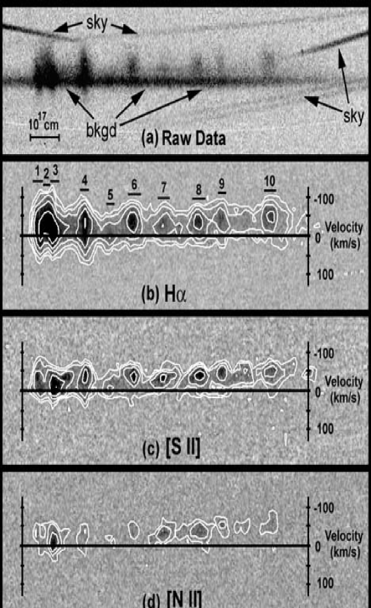
Figure 16: Position-velocity diagrams along the HH 110 jet. (a): A typical single 20-minute exposure corrected for distortion but not for background contamination. Night sky lines from adjacent orders are labeled, and the widths of these lines shows the instrumental spectral resolution. Emission from the molecular cloud, denoted as ‘bkgd’, defines zero radial velocity. (b): The H$\alpha$ position-velocity diagram, coadded from seven 20-minute exposures and with background subtracted. The numbered regions correspond to the areas along the slit marked in Fig. 15. The jet is easily resolved everywhere along the flow. Contours are separated by a factor of 1.41 in flux. (c) and (d): Same as (b) but for [S II] 6716+6731, and [N II] 6583, respectively.

Figs. 16 and 17 show that the H$\alpha$ emission line widths are larger than those of the forbidden lines. This behavior is expected because a component of H$\alpha$ occurs from collisional excitation immediately behind the shock front where the temperature is highest. The thermal FWHM of H$\alpha$ is given by

$$V_{th}=\left(V_{OBS}^{2}-V_{forb}^{2}\right)^{0.5}$$ (9)

where V_forb = (V${}_{NT}^{2}$ + V${}_{INST}^{2}$)^0.5 is the observed FWHM of the forbidden lines, V_NT the nonthermal FWHM and V_INST the instrumental FWHM.

We can use the thermal line width observation to measure the shock velocity in the gas. The temperature immediately behind a strong shock is given by

$$T={3\over 16}{\mu m_{H}V_{S}^{2}\over k}$$ (10)

where $\mu$ is the mean molecular weight of the gas and V_S is the shock velocity. The mean molecular weight depends on the preshock ionization fraction of the gas, and the postshock gas will have different ion and electron temperatures immediately behind the shock until the two fluids equilibrate (McKee, 1974), but the equilibration distance should be unresolved for HH 110. For simplicity we take the preshock gas to be mostly neutral, so $\mu$ $\sim$ 1. For thermal motion along the line of sight, the FWHM of a hydrogen emission line profile is then

$$V_{th}=2.354\left({kT\over{m_{H}}}\right)^{0.5}$$ (11)

Combining these two equations we obtain

$$V_{S}=0.98V_{th}$$ (12)

so the shock velocity is closely approximated by the observed thermal FWHM.

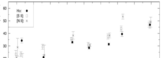
Figure 18: Kinematics of HH 110. Top: Blueshifted radial velocity of the regions along the slit marked in Fig. 15, measured relative to the HH 110 molecular cloud. The three emission lines shown for each region are offset slightly in the x-direction for clarity. Middle: Observed FWHM of the emission line profiles in Fig. 17. The H$\alpha$ linewidths are larger than those of the forbidden lines owing to thermal broadening. Bottom: Shock velocities inferred for each region, based on the thermal speed of H$\alpha$ in the postshock gas.

Fig. 18 summarizes the kinematics and dynamics within HH 110. The radial velocity gradually becomes more negative at distances greater than about $2\times 10^{17}$ cm. The radial velocities in the different emission lines track one another well. However, the same is not true for the line widths: both Fig. 17 and Fig. 18 show clearly that H$\alpha$ is broader than the forbidden line profiles. This behavior is expected because when the preshock gas is neutral, much of the H$\alpha$ comes from collisional excitation immediately behind the shock front where the temperature is high. The low atomic mass of H also increases its line width relative to those of N and S. The graph shows that the nonthermal component of the line profiles stays approximately constant at $\sim$ 40 km s^-1, and the thermal component of H$\alpha$ and the shock velocity are $\sim$ 50 km s^-1.

There are two epochs of HST images available (Reipurth PI), separated by about 22 months, and these data show intriguing and complex proper motions. Regions 1 through 4 have multiple shock fronts some of which move in the direction of the jet while others move along the deflected flow. Fig. 18 shows that this impact zone has higher nonthermal line widths than present in the flow downstream, consistent with the HST data. Throughout this rather broad region, denoted as such in Fig. 15, jet material impacts the molecular cloud. Hints of this behavior are evident in the ground based proper motion data of Lopez et al. (2005), which show proper motion vectors directed midway between the direction of the jet and that of the deflected flow.

Downstream from region 4, the material all moves in the direction of the deflected flow and gradually expands in size. The electron density of the shocked gas declines as the flow expands (Reipurth & Olberg, 1991). The slow increase in the blueshifted radial velocity could arise if the observer sees a concave cavity that gradually redirects the deflected flow towards our line of sight. One gets the impression from the HST images of a series of weak bubbles that emerges from the impact zone.

Published proper motion measurements (Lopez et al., 2005) suggest tangential velocities of $\sim$ 150 km s^-1 along the deflected flow. Hence, the nonthermal broadening is $\sim$ 25% of the bulk flow speed in the deflected jet, while the internal shock speeds are typically 30% of the flow speed. The temperature immediately behind a 50 km s^-1 shock is $\sim$ $5.7\times 10^{4}$ K, and will drop to $\lesssim$ 5000 K in areas where forbidden lines have cooled. The corresponding sound speeds are $\sim$ 20 km s^-1 and 8 km s^-1, respectively, so the bulk flow speed is $\sim$ Mach 10 in the deflected flow, while the internal shocks there are $\sim$ Mach 3 $-$ 6. The magnetosonic Mach numbers will be lower, depending on the field strength.

4.3 Wide-Field H₂ Images of the HH 110 Region

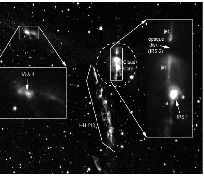
Figure 19: The HH 110 region, imaged in the H₂ 2.12$\mu$m line with the NEWFIRM camera. The HH 110 flow originates at the VLA 1 source (Choi & Tang, 2006) and radiates in H₂ after it deflects from a molecular cloud core. Two sources, IRS 1 and IRS 2, drive nearly parallel jets within the core itself. IRS 2 appears to be an opaque flared disk seen nearly edge-on.

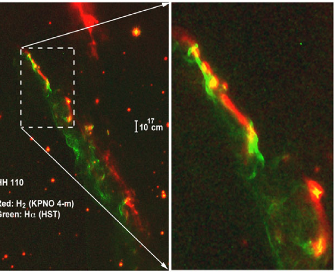
Figure 20: Image of H₂ (red, from NEWFIRM), and H$\alpha$ (green, from the Hubble Space Telescope archive) of HH 110. The H₂ emission is systematically offset to the right the H$\alpha$, consistent with material being dragged from the molecular cloud core by the glancing collision with a jet.

In order to better define how the HH 110 jet entrains material from the molecular cloud, and to verify that the deflected jet model is appropriate for this object, we obtained new wide-field near-infrared images of the region. In Figs. 19 and 20 we present a portion of an H₂ image taken 21 Sept., 2008 with the NEWFIRM infrared camera attached to the 4-m telescope at Kitt Peak National Observatory. The image was constructed from 20 individual dithers of 2 minutes apiece for a total exposure time of 40 minutes. The wide-field image in Fig. 19 shows VLA 1, the driving source of the HH 110 flow (Choi & Tang, 2006). The jet from this source, known as HH 270, does not radiate in H₂ until it strikes the molecular cloud, although the jet is visible in deep [S II] images (Choi & Tang, 2006).

Our H₂ image clearly shows two other jets that emanate from sources embedded within the molecular cloud core. IRS 1 (aka IRAS 05487+0255) is a bright near-IR source, while IRS 2 appears to be obscured by a flared disk seen nearly edge-on (as in HH 30, Burrows et al. (1996)). These sources drive a molecular outflow along the direction of the jets we see in the H₂ image (Reipurth & Olberg, 1991). Archival Spitzer images of the region at mid-infrared (3.6 $\mu$m $-$ 8 $\mu$m), and far-infrared (24 $\mu$m, 70 $\mu$m and 160 $\mu$m) wavelengths reveal three very bright sources that persist in all bands in the region, VLA 1, IRS 1, and IRS 2. The spectral energy distribution of IRS 1 is still rising at 100 $\mu$m, indicative of a heavily embedded source. The morphology of the HH 30 clone IRS 2 splits into two pieces at shorter wavelengths in the Spitzer images, consistent with an obscuring disk seen edge-on. Epoch 2000 coordinates for the midpoint of the HH 30-like disk in IRS 2 are 5:51:22.70 +2:56:05, and for IRS 1 are 5:51:22.60 +2:55:43.

The ubiquity of jets in this region is a common occurrence, as most star-forming regions have multiple sources that drive jets. However, it does potentially bring into question whether or not what we and others (e.g. Reipurth et al., 1996) interpret as a deflected jet for HH 110 may simply be a distinct flow generated by some other embedded source to the northeast of the emission. The counter to this argument is that Fig. 19 does not show a source near the apex of HH 110, and the Spitzer images of the region also show nothing there at mid-infrared wavelengths. If the hot H₂ is dragged out from the molecular cloud core by the impact of the jet, there should be a spatial offset between the H₂ from the core and the H$\alpha$ in the jet, with the H₂ located on the side of the spray closest to the core. The color composite in Fig. 20 demonstrates this effect very well, as noted previously for a small portion of the jet (Noriega-Crespo et al., 1996).

5 Connecting the Laboratory Experiments With Astrophysical Jets

Our laboratory results highlight two aspects of the fluid dynamics that are particularly useful for interpreting astronomical images and spectra $-$ entrainment of ambient material and the dynamics within contact discontinuities. The experiments also serve as a reminder that viewing angle affects how a bow shock appears in an image. We discuss each of these ideas below.

5.1 Interpretation of Astronomical Images

Keeping in mind that magnetic fields may play some role in the dynamics, we can look to the experiments as a guide to how material from an obstacle like a molecular cloud core becomes entrained by a jet in a glancing collision. As noted above, in the astronomical images the H₂ emission in Fig. 20 must arise from the cloud core to be consistent with the observed spatial offset of the H$\alpha$ and H₂, and the lack of H₂ in the jet before it strikes the cloud. In the experiments, the jet entrains material in the ball in part because the flute penetrates into the ball and ‘scoops up’ whatever material falls within the flute (Fig. 4). This type of entrainment is probably of little interest astrophysically because its origin is unique to the relatively hollow density structure within the experimental jet. However, material from the ball is also lifted into the flow because the jet penetrates into the ball along the contact discontinuity. Both the radiographs and the RAGE simulations show this region to be highly structured (Figs. 3-5). The experiments indicate that once a part of the jet becomes deflected into the ball along the contact discontinuity it creates a small cavity where the jet material lifts small fragments of the ball into the flow. We see the same morphology in the astrophysical case. This type of entrainment is one that occurs as a natural outgrowth of the complex 3-D structure along a contact discontinuity.

As Fig. 6 shows, the deflected bow shock appears much wider when the bow shock has a significant component along the line of sight. While this result is rather elementary, Fig. 6 provides a graphic example that is important to keep in mind when interpreting astronomical images of bow shocks when the shocked gas has a large redshift or blueshift. In such cases a flow may appear to be much less collimated than if one were to observe the bow shock perpendicular to its direction of motion. An example of a wide bow shock oriented at a large angle from the plane of the sky is HH 32A, which has been thoroughly studied at optical wavelengths (Beck et al., 2004).

5.2 Filamentary Structures in the Experiment and the Astronomical Observations

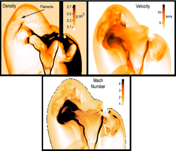
Figure 21: RAGE simulations of the dynamics within the deflected experimental jet. The figure shows the density, velocity, and local Mach number at each point within the plane of symmetry of the experiment at 200 ns. The filaments within the working surface of the deflected bow shock are discussed in the text.

The working surface of the deflected bow shock in the experiment exhibits an intriguing filamentary structure in the observed radiographs and in the RAGE simulations (Figs. 3 and 21) that resembles the filamentary shock waves seen in HH 110 (Fig. 15). If differential motions between adjacent filaments in the working surface are supersonic, then weak shocks like those seen in HH 110 could form as the filaments interact at later times.

To test this idea, we generated synthetic images of the Mach number and the velocity along a plane that contains the center of the ball in Fig. 21. Together, these two images indicate whether shock waves are likely to form within the working surface at later times. Neither image alone provides this information: a constant velocity flow with two adjecent regions of different temperature will show markedly different Mach numbers in close proximity but will not create a shock; similarly, a shock will only form between adjacent fluid elements with differing velocities and the same temperature if the difference between the Mach numbers exceeds unity.

Velocity differences between the filaments in the working surface in Fig. 21 are typically 1 $-$ 2 km/s, or only about 10% of the initial jet velocity. In contrast, the shock waves in HH 110 have higher velocities, about 30% of the jet speed (section 4.2; Fig. 18). Moreover, Mach numbers in the filaments range from $\sim$ 1 $-$ 2, so differences between the filaments are $\lesssim$ 1, indicating that the relative motions between the filaments are subsonic. We conclude that the velocity differences between the filaments in the working surface are too low to form shock waves unless the filaments cool. Even if that were to occur, the shock velocities will be about a factor of three smaller relative to the jet speed than those seen in HH 110. Hence, the best explanation for the shocks observed in HH 110 is that the source is impulsive, where each pulse impacts the molecular cloud in a similar manner to our experimental setup.

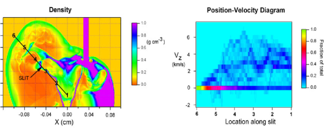
Figure 22: Synthetic position-velocity diagram of the laser experiment. The density image at left is a slice through the symmetry plane (z=0), which by definition contains the axis of the jet and the center of the ball. Negative values of z are into the paper. At each position (x_∘,y_∘) along the ‘slit’, the position-velocity diagram at right gives a probability distribution for the radial velocity V_Z of material located at (x_∘, y_∘, z$<$0). The large amount of material at V_Z=0 simply represents undisturbed foam. Material at (x_∘, y_∘, z$>$0) produces an identical p-v diagram (not shown) but with the sign of V_Z reversed.

It is instructive to consider what one might observe in a position-velocity diagram in the experiment, were it possible to align a slit down the axis of the deflected flow and obtain a velocity-resolved spectrum, as is possible with astronomical observations. We show this exercise in Fig. 22, where we have simply assumed the emissivity of the gas to be proportional to its density. For a real emission line the emissivity depends on the temperature, density, and ionization state of the gas in a complex manner determined by the atomic physics of the line. However, it is still instructive to see what sort of morphologies appear in a p-v diagram of this sort.

The synthetic p-v diagram in Fig. 22 contains a series of arcs that resemble those present in astronomical slit spectra of spatially-resolved bow shocks (Raga & Böhm, 1986; Hartigan et al., 1990). These arcs occur when the slit crosses the jet or an interface such as the cavity evacuated by the jet. In the case of spatially resolved bow shocks, arcs in the p-v diagram result from the motion of a curved shell of material, where the orientation of the velocity vector relative to the observer changes along the slit. The lesson from the experiment seems to be that in highly structured flows like our deflected jet, curved cavities and filaments naturally produce p-v diagrams that contain multiple arcuate features. As in the case of resolved bow shocks, the velocity amplitude of the arcs in the p-v diagram is on the order of the shock velocity responsible for the arc.

In an optically thin astrophysical nebula one can measure five out of the six phase space dimensions: x and y position on the sky from images, proper motion velocities V_x and V_y from images taken at two times, and the radial velocity V_z along the line of sight from spectroscopy. As we have shown above, V_z is an extremely useful diagnostic of the dynamics of a flow, but one that is currently not possible to measure in laboratory experiments. If such a diagnostic instrument could be developed it would open up a wide range of possibilities for new studies of supersonic flows.

6 Summary and Future Work

The combination of experimental, numerical and astronomical observational data from this study demonstrates the potential of the emerging field of laboratory astrophysics. In this paper we have studied how a supersonic jet behaves with time as it deflects from an obstacle situated at various distances from the axis of the jet. The laboratory analog of this phenomenon scales very well to the astrophysical case of a stellar jet which deflects from a molecular cloud core. An important component to our study was to expand the observational database of best astrophysical example, HH 110, by obtaining new spatially-resolved high-spectral resolution observations capable of distinguishing thermal motions from turbulent motions, and by acquiring a new deep infrared H₂ image that can be compared with existing optical emission line images from the Hubble Space Telescope.

The laboratory experiments span a range of times, spatial offsets between the axis of the jet and the center of the ball (impact parameters), viewing angles, opacities (backlighters), and materials. The experiments are reproducible and do not depend on composition or structure of foam, or on the pinhole diameter of the backlighter (spatial resolution of the experiment). Synthetic radiographs of the experiment from RAGE match the experimental data extremely well, both qualitatively as images and quantiatively with Fourier analysis. In fact, the agreement is so good that we have used the synthetic velocity maps from RAGE to compare the internal dynamics of the experiment with those that we measure from the new spectral maps of HH 110.

A new wide-field H₂ image supports a scenario where HH 110 represents the shocked ‘spray’ that results from a glancing collision of the HH 270 jet with a molecular cloud core. The H₂ in HH 110 is offset from the H$\alpha$ toward the side closest to the molecular core, consistent with the deflected jet model. The H₂ images also uncovered two sources within the core that drive collimated jets, one a bright near-infrared source, and the other a highly-obscured source that appears to be a dense protostellar disk observed nearly edge-on, as in HH 30.

The experiments provide several important insights into how deflected supersonic jets like HH 110 behave. In the experiment, entrainment of material in the obstacle occurs in part because the morphology of the contact discontinuity between the shocked jet and shocked obstacle easily develops a complex 3-D structure of cavities that enables the jet to isolate clumps of obstacle material and entrain them into the flow. A similar process likely operates in HH 110. The experiments also reveal filamentary structure in the working surface area of the deflected bow shock, but the relative motion between these filaments is subsonic. Hence, while this dynamical process will generate density fluctuations in the outflowing gas, it cannot produce the filamentary structure and $\sim$ Mach 5 shocks shown by the new velocity maps of HH 110. For this reason the best model for HH 110 remains that of a pulsed jet which interacts with a molecular cloud core.

Synthetic position-velocity maps along the deflected jet from the RAGE simulations of the experiments appear as a series of arcs, similar to those observed in astronomical observations of resolved bow shocks. A close examination of the experimental data shows that these arcs correspond to regions where the slit crosses different regions of the flow, such as cavities evacuated by the jet, the jet itself, or entrained material from the ball. This correspondance between the appearance of a p-v diagram and the actual morphology of a complex flow is an intuitive, although perhaps unexpected result of studying the dynamics within the experimental flow.

Finally, observations of the deflected bow shock from different viewing angles emphasize that the observed morphology and collimation properties of bow shocks depend strongly upon the orientation of the flow with respect to the observer. As one would expect, a bow shock deflected toward the observer appears less collimated than one that is redirected into the plane of the sky. The impact parameter of the jet and obstacle determines how much the jet deflects from the obstacle and how rapidly the obstacle becomes disrupted by the jet.

While experimental analogs of astrophysical jets are highly unlikely to ever reproduce accurate emission line maps, laser experiments can provide valuable insights into how the dynamics of complex flows behave. Our study of a deflected supersonic jet is only one example of how the fields of astrophysics, numerical computation, and laboratory laser experiments can compliment one another. We are currently embarking on a similar program to study the dynamics within supersonic flows that are highly clumpy, and other investigations are underway related to the launching and collimation of jets (Bellan et al., 2009).

Table 1:

Fluid Parameter	HH 110	Experiment
L (cm) [jet size]	1e15	0.02
V (km s-1) [jet velocity]	150	10
$\rho$ (g cm-3) [jet density]	2e-20	1
P (dyne cm-2) [jet pressure]	1e-8	3e10
tflow (sec) [flow timescale]	3e9	1e-7
Composition	H	Ti
T (eV) [temperature of wake]	0.6	1
Euler number in jet	22	6
$\nu_{mat}$ (cm2s-1) [viscosity]	9e13	2e-5
$\nu_{rad}$ (cm2s-1) [viscosity]	2e21	1e-12
$\nu_{c}$ (s-1) [collision freq]	0.002	2e13
$\chi$ (cm2s-1) [diffusivity]	5e24	5e-18
Remat [Reynolds number]	7e8	1e9
Pemat [Peclet number]	1e7	3e4
$\lambda_{mat}$ (cm) (mean-free path)	3e8	8e-9
$\lambda_{rad}$ (cm) (mean-free path)	$>>$La	3e-5
$\tau_{mat}$ [optical depth]	9e6	2e6
$\tau_{rad}$ [optical depth]	$<<$1a	7e2
Bo#	$>$1e3	2e4

References

- Ampleford al. (2007) Ampleford, D., et al. 2007, Ap&SS 307, 29
- Balick & Frank (2002) Balick, B., & Frank, A. 2002, ARA&A 40, 439
- Beck et al. (2004) Beck, T., Riera, A., Raga, A., & Aspin, C. 2004, AJ 127, 408
- Bellan et al. (2009) Bellan, P. et al. 2009, Phys. Plasmas 16, 41005
- Blondin et al. (1990) Blondin, J., Fryxell, B., & Königl, A. 1990, ApJ 360, 370
- Brugle et al. (1981) Brugel, E., Böhm, K.-H., & Mannery, E. 1981, ApJS 47, 117
- Burrows et al. (1996) Burrows, C., et al. 1996, ApJ 473, 437
- Cabrit (2007) Cabrit, S. 2007, Proceedings of the IAU Symposium 243, J. Bouvier & I. Appenzeller eds., (Cambridge:Cambridge University Press), 203
- Carver et al. (2009) Carver, R., et al. 2009, in preparation.
- Cerqueira et al. (2006) Cerqueira, A., Velazquez, P., Raga, A., Vasconcelos, M. & de Colle, F. 2006, A&A 448, 231
- Choi & Tang (2006) Choi, M., & Tang, Y.-W. 2006, ApJ 648, 504
- Coker et al. (2007) Coker, R. F. et al. 2007, Ap&SS 307, 57
- Colella (1985) Colella, P. 1985, SIAM J. Comput. 6, 104
- Cunningham et al. (2006) Cunningham, A.J., Frank, A., & Blackman, E.G. 2006, ApJ, 646, 1059
- Drake et al. (2006) Drake, R.P., Davison, L., & Horie, Y. 2006, “High-Energy-Density Physics: Fundamentals, Inertial Fusion, and Experimental Astrophysics” (Berlin:Springer).
- Drake et al. (2009) Drake, P., Kuranz, C., Miles, A., Muthsam, H., & Plewa, T. 2009, Phys. Plasmas 16, 41004
- Cunningham et al. (2008) Cunningham, A. J., Frank, A., Varniere, P., Mitran, S., & Jones, T. W. 2008, ArXiv e-prints, 710, arXiv:0710.0424
- Ferreira et al. (2006) Ferreira, J., Dougados, C., & Cabrit, S. 2006, A&A 453, 785
- Foster et al. (2002) Foster, J. M. et al. 2002, Phys. Plasmas 9, 2251
- Foster et al. (2005) Foster, J. M. et al. 2005, ApJ 634, L77
- Gittings (2008) Gittings, M., et al. 2008, Comput. Sci. Disc. 1, 15005
- Hansen et al. (2007) Hansen, J. F., Robey, H. F., Klein, R. I., & Miles, A. R. 2007, ApJ 662, 379
- Harris and Krawczynski (2006) Harris, D., & Krawzynski, H. 2006, ARA&A 44, 463
- Hartigan (2008) Hartigan, P. 2008, Lecture Notes in Physics 742, 15
- Hartigan et al. (1995) Hartigan, P., Edwards, S., & Ghandour, L. 1995, ApJ 452, 736
- Hartigan et al. (2004) Hartigan, P., Edwards, S., & Pierson, R. 2004, ApJ 609, 261
- Hartigan et al. (2007) Hartigan, P., Frank, A., Varniere, P., & Blackman, E. 2007, ApJ 661, 910
- Hartigan et al. (1995) Hartigan, P., Morse, J., & Raymond, J. 1995, ApJ 444, 943
- Hartigan et al. (2000) Hartigan, P., Morse, J., Palunas, P., Bally, J., & Devine, D. 2000, AJ 119, 1872
- Hartigan et al. (2001) Hartigan, P., Morse, J., Reipurth, B., Heathcote, S. & Bally, J. 2001, ApJ 559, L157
- Hartigan et al. (1987) Hartigan, P., Raymond, J., & Hartmann, L. 1987, ApJ 316, 323
- Hartigan et al. (1990) Hartigan, P., Raymond, J., & Meaburn, J. 1990, ApJ 362, 624
- Heathcote et al. (1996) Heathcote, S., Morse, J., Hartigan, P., Reipurth, B., Schwartz, R., Bally, J., & Stone, J. 1996, AJ 112, 1141
- Heathcote & Reipurth (1992) Heathcote, S., & Reipurth, B. 1992, AJ 104, 2193
- Henke et al. (1986) Henke, B. L., Uejio, J., Y., Stine, G., F., Dittmore, C., H., & Fujiwara, F. G. 1986, J. Opt. Soc. Am. B 3, 1540
- Krause (2003) Krause, M. 2003, A&A 398, 113
- Kuranz et al. (2007) Kuranz, C. et al. 2007, Ap&SS 307, 115
- Landau & Lifshitz (1987) Landau, L., & Lifshitz, E. 1987, Fluid Mechanics, (Oxford:Pergamon)
- Lebedev et al. (2004) Lebedev, S., et al. 2004, ApJ 616, 988
- Loupias et al. (2007) Loupias, B. et al. 2007, PRL 99, 265001
- Lopez et al. (2005) Lopez, R., Estalella, R., Raga, A., Reira, A., Reipurth, B., & Heathcote, S. 2005, A&A 432, 567
- McKee (1974) McKee, C. 1974, ApJ 188, 335
- Mirabel & Rodriguez (1999) Mirabel, I., & Rodriguez, L. 1999, ARA&A 37, 409
- Morse et al. (1992) Morse, J., Hartigan, P., Cecil, G., Raymond, J., & Heathcote, S. 1992, ApJ 399, 231
- Mottura (1997) Mottura, L. 1997, J. Comp. Phys. 138, 354
- Noriega-Crespo et al. (1996) Noriega-Crespo, A., Garnavich, P., Raga, A., Canto, J., & Böhm, K.-H. 1996, ApJ 462, 804
- Raga & Böhm (1986) Raga, A., & Böhm, K.-H. 1986, ApJ 308, 829
- Ray et al. (2007) Ray, T., Dougados, C., Bacciotti, F., Eislöffel, J., & Chrysostomou, A. 2007, in “Protostars & Planets V”, B. Reipurth, D. Jewitt, & K. Keil eds., (Tucson:Univ. of Arizona Press)
- Reighard & Drake (2007) Reighard, A. & Drake, R. 2007, Ap&SS 307, 121
- Remington et al. (2006) Remington, B., Drake, P., & Ryutov, D. 2006, Rev. Mod. Phys. 78, 755
- Riera et al. (2003) Riera, A., Raga, A., Reipurth, B., Amram, P., Boulesteix, J., Canto, J., & Toledano, O. 2003, AJ 126, 327
- Reipurth & Olberg (1991) Reipurth, B., & Olberg, M. 1991, A&A 246, 535
- Reipurth & Bally (2001) Reipurth, B., & Bally, J. 2001, ARA&A 39, 403
- Reipurth et al. (1996) Reipurth, B., Raga, A., & Heathcote, S. 1996, A&A 311, 989
- Ryutov et al. (1999) Ryutov, D., Drake, R., Kane, J., Liang, E., Remington, B. & Wood-Vasey, W. 1999, ApJ 518, 821
- Rosen et al. (2006) Rosen, P. A. et al. 2006, J. Phys. IV France 133, 1019
- Soures et al. (1996) Soures, J., et al. 1996, Phys. Plasmas 3, 218
- Schwartz (1978) Schwartz, R. 1978, ApJ 223, 884