On the global well-posedness of a class of Boussinesq- Navier-Stokes systems

Abstract

In this paper we consider the following 2D Boussinesq-Navier-Stokes systems

$$\begin{split}\partial_{t}u+u\cdot\nabla u+\nabla p+|D|^{\alpha}u&=\theta e_{2}\\ \partial_{t}\theta+u\cdot\nabla\theta+|D|^{\beta}\theta&=0\quad\end{split}$$

with $\textrm{div}u=0$ and $0<\beta<\alpha<1$. When $\frac{6-\sqrt{6}}{4}<\alpha<1$, $1-\alpha<\beta\leq f(\alpha)$, where $f(\alpha)$ is an explicit function as a technical bound, we prove global well-posedness results for rough initial data.

Mathematics Subject Classification (2000): 76D03, 76D05, 35B33, 35Q35
Keywords: Boussinesq system, regularization effect, paradifferential calculus, global well-posedness.

1 Introduction

The 2D generalized Boussinesq systems are of the forms

$$\begin{cases}\partial_{t}u+u\cdot\nabla u+\nabla p+\nu|D|^{\alpha}u=\theta e_{2},\quad(t,x)\in\mathbb{R}^{+}\times\mathbb{R}^{2}\\ \partial_{t}\theta+u\cdot\nabla\theta+\kappa|D|^{\beta}\theta=0\\ \textrm{div}u=0\\ u|_{t=0}=u^{0},\quad\theta|_{t=0}=\theta^{0},\end{cases}$$ (1.1)

where $\nu\geq 0,\kappa\geq 0$, $(\alpha,\beta)\in[0,2]^{2}$ and $|D|^{\alpha}$ is defined via the Fourier transform

$$\mathcal{F}(|D|^{\alpha}f)(\xi)=|\xi|^{\alpha}\mathcal{F}(f)(\xi).$$

These systems are simple models widely used in the modeling of the oceanic and atmospheric motions (see e.g.[16]). Here, the divergence-free vector field $u=(u^{1},u^{2})$ denotes the velocity, scalar functions $\theta$, $p$ denote the temperature and the pressure respectively, the absolute constants $\nu,\kappa$ can be seen as the inverse of Reynolds numbers. The term $\theta e_{2}$ in the velocity equation, with $e_{2}$ the canonical vector $(0,1)$, models the effect of gravity on the fluid motion. If $\theta^{0}=0$, the systems are reduced to the 2D generalized Navier-Stokes(Euler) equations. Clearly, due to the maximum principle for the vorticity and the B-K-M criterion in [2], smooth solutions of these two-dimensional systems are global in time.

From a mathematical view, the fully viscous model with $\nu>0,\kappa>0,\alpha=\beta=2$ is the simplest one to study. It acts very similar to the 2D Navier-Stokes equation and similar global results can be achieved. On the other hand, the most difficult one for the mathematical study is the inviscid model, that is when $\nu=\kappa=0$. Up to now, only local existence results can be proven.

Here we focus on the cases where the dissipation effect in the velocity equation plays a dominant role. The most typical models are those with the diffusion effect in the temperature equation neglected ($\kappa=0,\nu>0$), and there have been some recent important works on these Boussinesq systems. For the case with the full viscosity, i.e. when $\alpha=2$, global well-posedness results can be established in various functional spaces. In [3], Chae proved that for large initial data $(u^{0},\theta^{0})\in H^{s}\times H^{s}$ with $s>2$ the system is global well-posed. See also [13]. Later on, Hmidi-Keraani in [10] showed global well-posedness for less regular data $(u^{0},\theta^{0})\in H^{s}\times H^{s}$ with $s>0$. In [8], Danchin-Paicu proved the unconditional uniqueness in the energy space $L^{2}\times L^{2}$. For the case with weaker dissipation, i.e. when $1\leq\alpha<2$, the problem is also solvable. When $\alpha\in]1,2[$, as in [10] through taking advantage of the maximal regularity estimates for the semi-group $e^{-t|D|^{\alpha}}$, one can prove the global well-posedness. For the subtle critical case $\alpha=1$, Hmidi-Keraani-Rousset in [11] proved the global result for the rough data through exploiting the new structural properties of the system solved by vorticity $\omega$ and temperature $\theta$.

One natural problem is how to establish the global well-posedness for the problem (1.1) when we further weaken the dissipation effect in the velocity equation to the $\alpha<1$ case. It seems that introducing the diffusion effect in the temperature equation ($\kappa>0$) is necessary and meanwhile $\beta$ should satisfy $\beta\geq 1-\alpha$. In fact, we have a rough observation from the coupling system of temperature $\theta$ and vorticity $\omega$, where $\omega$ is defined by $\omega:=\mathrm{curl}u=\partial_{1}u^{2}-\partial_{2}u^{1}$. The coupling system writes

$$\begin{cases}\partial_{t}\omega+u\cdot\nabla\omega+\nu|D|^{\alpha}\omega=\partial_{1}\theta,\\ \partial_{t}\theta+u\cdot\nabla\theta+\kappa|D|^{\beta}\theta=0,\\ \omega|_{t=0}=\omega^{0}:=\mathrm{curl}u^{0},\quad\theta|_{t=0}=\theta^{0}.\end{cases}$$

To get the key uniform estimates on $\omega$, the smoothing effect from the dissipation term should at least roughly compensate the loss of one derivative in $\theta$ in the vorticity equation with the help of the diffusion effect in the temperature equation, from which $\beta$ derivative in $\theta$ is gained. Hence $\alpha+\beta\geq 1$ is needed. This is also the sense in which the case $\{\alpha=1,\nu>0,\kappa=0\}$ is called as a critical case.

Our goal in this paper is to understand the coupling effects between the dissipative terms which come both in the velocity equation and the temperature equation, and their effects on the global existence, see Figure I. For brevity, we always set $\nu=\kappa=1$ in the sequel. We will modify the elegant argument introduced in [11] and [12] to study the the global well-posedness of (1.1) with $0<\beta<\alpha<1$. More precisely, our main result is the following

Theorem 1.1.

Let $(\alpha,\beta)\in\Pi:=\big{]}\frac{6-\sqrt{6}}{4},1\big{[}\times\big{]}1-\alpha,\min\{\frac{7+2\sqrt{6}}{5}\alpha-2,\frac{\alpha(1-\alpha)}{\sqrt{6}-2\alpha},2-2\alpha\}\big{]}$ (for $\Pi$ see Figure 1 in the sequel), $\theta^{0}\in H^{1-\alpha}\cap B^{1-\alpha}_{\infty,1}$ and $u^{0}$ be a divergence-free vector field belonging to $H^{1}\cap\dot{W}^{1,p}$ with $p\in]\frac{2}{\beta+\alpha-1},\infty[$. Then the system (1.1) has a unique global solution $(u,\theta)$ such that for every $\sigma\in[1,\frac{\alpha}{1-\alpha+2/p}[$,

$$u\in L^{\infty}(\mathbb{R}^{+},H^{1}\cap\dot{W}^{1,p})\cap L^{\sigma}_{loc}(\mathbb{R}^{+},B^{1}_{\infty,1})\quad and\quad\theta\in L^{\infty}(\mathbb{R}^{+},H^{1-\alpha}\cap B^{1-\alpha}_{\infty,1}).$$

Remark 1.1.

Note that the case $\{\nu=\kappa=1,\alpha=1,\beta=0\}$ shares almost the same nature with the partially inviscid case $\{\nu=1,\kappa=0,\alpha=1\}$ studied in [11], and the same method can be applied only by treating the damping term $\theta$ in the temperature equation as a harmless forcing term. Our results are motivated by this additional point and generalize the critical limiting case to the perturbed cases. This point is also the reason why the upper bound of $\beta$ occurs.

The main idea in the proof of Theorem 1.1 is to use the internal structures of the system solved by $(\omega,\theta)$, which is analogous to [11, 12]. To get a first glance, we will neglect the nonlinear term here, then the coupling system of $(\omega,\theta)$ reduces to

$$\partial_{t}\omega+|D|^{\alpha}\omega=\partial_{1}\theta,\quad\partial_{t}\theta+|D|^{\beta}\theta=0.$$

Thus

$$\partial_{t}\omega+|D|^{\alpha}(\omega-|D|^{-\alpha}\partial_{1}\theta)=0,\quad\partial_{t}\theta+|D|^{\beta}\theta=0.$$

Set $R_{\alpha}:=|D|^{-\alpha}\partial_{1}$, then

$$\partial_{t}(\omega-R_{\alpha}\theta)+|D|^{\alpha}(\omega-R_{\alpha}\theta)=|D|^{\beta-\alpha}\partial_{1}\theta,\quad\partial_{t}\theta+|D|^{\beta}\theta=0.$$

If roughly $\alpha\thicksim 1$, $\beta\thicksim 0$, the forcing term $|D|^{\beta-\alpha}\partial_{1}\theta$ has much less loss of derivative than term $\partial_{1}\theta$ and indeed we have some good estimates on $\omega-R_{\alpha}\theta$. These estimates will strongly help to obtain the needful estimates on $\omega$.

To prove Theorem 1.1, we shall study the new equation to get a priori estimates on $\omega-R_{\alpha}\theta$ and then return to obtain crucial a priori estimates on $\omega$. During this process, some technical difficulty will be encountered. The first one is to estimate the commutator $[R_{\alpha},u\cdot\nabla]$ which naturally turns up when the nonlinear term is taken into account; another one is to obtain estimates on $\omega$ from estimates on $\omega-R_{\alpha}\theta$ (since in contrast with the Riesz transform, $R_{\alpha}$ is not $L^{p}$-bounded and roughly contains positive derivative of $1-\alpha$ power). We shall treat such commutator estimates in Section 3 and yet we shall sufficiently use the smooth effect (Proposition 2.3) of the temperature equation to overcome the another difficulty.

The paper is organized as follows. Section 2 is devoted to present some preparatory results on Besov spaces. Some estimates about linear transport-diffusion equation are also given. In Section 3, commutator estimates involving $R_{\alpha}$ are studied. Section 4 is the main part dedicated to the proof of Theorem 1.1. Finally, some technical lemmas are shown in Section 5.

2 Priliminaries

2.1 Notations

Throughout this paper the following notations will be used.
$\bullet$ The notion $X\lesssim Y$ means that there exist a positive harmless constant $C$ such that $X\leq CY$. $X\thickapprox Y$ means that both $X\lesssim Y$ and $Y\lesssim X$ are satisfied.
$\bullet$ $\mathcal{S}$ denotes the Schwartz class, $\mathcal{S}^{\prime}$ the space of tempered distributions, $\mathcal{S}^{\prime}/\mathcal{P}$ the quotient space of tempered distributions which modulo polynomials.
$\bullet$ We use $\mathcal{F}f$ or $\widehat{f}$ to denote the Fourier transform of a tempered distribution $f$.
$\bullet$ For any pair of operators $A$ and $B$ on some Banach space $\mathcal{X}$, the commutator $[A,B]$ is defined by $AB-BA$.
$\bullet$ For every $k\in\mathbb{Z}^{+}$, the notion $\Phi_{k}$ denotes any function of the form

$$\Phi_{k}(t)=C_{0}\underbrace{\exp(\ldots\exp}_{k\;times}(C_{0}t)\ldots),$$

where $C_{0}$ depends on the related norms of the initial data and its value may be different from line to line up to some absolute constants.

2.2 Littlewood-Paley decomposition and Besov spaces

To define Besov space we need the following dyadic unity partition (see e.g. [4]). Choose two nonnegative radial functions $\chi$, $\varphi\in C^{\infty}(\mathbb{R}^{n})$ be supported respectively in the ball $\{\xi\in\mathbb{R}^{n}:|\xi|\leq\frac{4}{3}\}$ and the shell $\{\xi\in\mathbb{R}^{n}:\frac{3}{4}\leq|\xi|\leq\frac{8}{3}\}$ such that

$$\chi(\xi)+\sum_{j\geq 0}\varphi(2^{-q}\xi)=1,\quad\forall\xi\in\mathbb{R}^{n};\qquad\sum_{q\in\mathbb{Z}}\varphi(2^{-q}\xi)=1,\quad\forall\xi\neq 0.$$

For all $f\in\mathcal{S}^{\prime}(\mathbb{R}^{n})$ we define the nonhomogeneous Littlewood-Paley operators

$$\Delta_{-1}f:=\chi(D)f;\;\forall q\in\mathbb{N}\quad\Delta_{q}f:=\varphi(2^{-q}D)f\;\;\mathrm{and}\;S_{q}f:=\sum_{-1\leq j\leq q-1}\Delta_{j}f.$$

The homogeneous Littlewood-Paley operators are defined as follows

$$\forall q\in\mathbb{Z},\quad\dot{\Delta}_{q}f:=\varphi(2^{-q}D)f,\quad\dot{S}_{q}f:=\sum_{j\leq q-1}\dot{\Delta}_{j}f.$$

The paraproduct between two distributions $f$ and $g$ is defined by

$$T_{f}g:=\sum_{q\in\mathbb{N}}S_{q-1}f\Delta_{q}g.$$

Thus we have the following formal decomposition known as Bony’s decomposition

$$fg=T_{f}g+T_{g}f+R(f,g),$$

where

$$R(f,g):=\sum_{q\geq-1}\Delta_{q}f\widetilde{\Delta}_{q}g,\quad\textrm{and}\quad\widetilde{\Delta}_{q}:=\Delta_{q-1}+\Delta_{q}+\Delta_{q+1}.$$

Now we introduce the definition of Besov spaces . Let $(p,r)\in[1,\infty]^{2}$, $s\in\mathbb{R}$, the nonhomogeneous Besov space $B^{s}_{p,r}$ is defined as the set of tempered distribution $f$ such that

$$\left\|f\right\|_{B^{s}_{p,r}}:=\left\|2^{qs}\left\|\Delta_{q}f\right\|_{L^{p}}\right\|_{\ell^{r}}<\infty,$$

The homogeneous space $\dot{B}^{s}_{p,r}$ is the set of $f\in\mathcal{S}^{\prime}(\mathbb{R}^{n})/\mathcal{P}(\mathbb{R}^{n})$ such that

$$\left\|f\right\|_{\dot{B}^{s}_{p,r}}:=\left\|2^{qs}\left\|\dot{\Delta}_{q}f\right\|_{L^{p}}\right\|_{\ell^{r}(\mathbb{Z})}<\infty.$$

We point out that for all $s\in\mathbb{R}$, $B^{s}_{2,2}=H^{s}$ and $\dot{B}^{s}_{2,2}=\dot{H}^{s}$.

Next we introduce two kinds of coupled space-time Besov spaces. The first one $L^{\varrho}([0,T],B^{s}_{p,r})$, abbreviated by $L^{\varrho}_{T}B^{s}_{p,r}$, is the set of tempered distribution $f$ such that

$$\left\|f\right\|_{L^{\varrho}_{T}B^{s}_{p,r}}:=\left\|\left\|2^{qs}\left\|\Delta_{q}f\right\|_{L^{p}}\right\|_{\ell^{r}}\right\|_{L^{\varrho}_{T}}<\infty.$$

The second one $\widetilde{L}^{\varrho}([0,T],B^{s}_{p,r})$, abbreviated by $\widetilde{L}^{\varrho}_{T}B^{s}_{p,r}$, is the set of tempered distribution $f$ satisfying

$$\left\|f\right\|_{\widetilde{L}^{\varrho}_{T}B^{s}_{p,r}}:=\left\|2^{qs}\left\|\Delta_{q}f\right\|_{L^{\varrho}_{T}L^{p}}\right\|_{\ell^{r}}<\infty.$$

Due to Minkowiski inequality, we immediately obtain

$$L^{\varrho}_{T}B^{s}_{p,r}\hookrightarrow\widetilde{L}^{\varrho}_{T}B^{s}_{p,r},\;if\;r\geq\rho\quad and\quad\widetilde{L}^{\varrho}_{T}B^{s}_{p,r}\hookrightarrow L^{\varrho}_{T}B^{s}_{p,r},\;if\;\varrho\geq r$$

We can similarly extend to the homogeneous ones $L^{\varrho}_{T}\dot{B}^{s}_{p,r}$ and $\widetilde{L}^{\varrho}_{T}\dot{B}^{s}_{p,r}$.

Berstein’s inequality is fundamental in the analysis involving Besov spaces (see e.g. [4])

Lemma 2.1.

Let $\mathcal{B}$ is a ball, $\mathcal{C}$ is a ring, $0\leq a\leq b\leq\infty$. Then for $k\in\mathbb{R}^{+}$, $\lambda>0$ there exists a constant $C>0$ such that

$$\left\||D|^{k}f\right\|_{L^{b}}\leq C\lambda^{k+n(\frac{1}{a}-\frac{1}{b})}\left\|f\right\|_{L^{a}}\quad if\;\textrm{supp}\;\mathcal{F}f\subset\lambda\mathcal{B},$$

$$C^{-1}\lambda^{k}\left\|f\right\|_{L^{a}}\leq\left\||D|^{k}f\right\|_{L^{a}}\leq C\lambda^{k}\left\|f\right\|_{L^{a}}\quad if\;\textrm{supp}\,\mathcal{F}f\subset\lambda\mathcal{C}.$$

2.3 Transport-diffusion Equation

In this subsection we shall collect some useful estimates for the smooth solutions of the following linear transport-diffusion equation

$$(TD)_{\beta}\quad\begin{cases}\partial_{t}\theta+u\cdot\nabla\theta+|D|^{\beta}\theta=f,\quad\beta\in[0,1]\\ \textrm{div}u=0,\quad\theta|_{t=0}=\theta^{0}.\end{cases}$$

The $L^{p}$ estimate for (TD)_β equation is shown in [6]

Proposition 2.2.

Let $u$ be a smooth divergence-free vector field of $\mathbb{R}^{n}$ and $\theta$ be a smooth solution of (TD)_β. Then for every $p\in[1,\infty]$ we have

$$\left\|\theta(t)\right\|_{L^{p}}\leq\left\|\theta_{0}\right\|_{L^{p}}+\int^{t}_{0}\left\|f(\tau)\right\|_{L^{p}}\,\textrm{d}\tau.$$ (2.1)

The following smoothing effect is important in the proof.

Proposition 2.3.

Let $u$ be a smooth divergence-free vector field of $\mathbb{R}^{n}$ with vorticity $\omega$ and $\theta$ be a smooth solution of (TD)_β. Then for every ($p,\varrho$)$\in[2,\infty[\times[1,\infty]$ we have

$$\mathrm{sup}_{q\in\mathbb{N}}2^{q\frac{\beta}{\varrho}}\left\|\Delta_{q}\theta\right\|_{L^{\varrho}_{t}L^{p}}\lesssim_{\varrho,p}\left\|\theta^{0}\right\|_{L^{p}}+\left\|\theta^{0}\right\|_{L^{\infty}}\left\|\omega\right\|_{L^{1}_{t}L^{p}}+\left\|f\right\|_{L^{1}_{t}L^{p}}.$$

Remark 2.1.

For $\varrho=1$, $\beta=1$ and $f=0$, the result has appeared in [12]. Here with necessary modifications, this generalized case can be treated in a similar way.

We also have the classical regularization effects as follows (see e.g. [15, 11, 9]).

Proposition 2.4.

Let $-1<s<1$, $\varrho_{1}\leq\varrho$, $(p,r)\in[1,\infty]^{2}$ and $u$ be a divergence-free vector field belonging to $L^{1}_{\textrm{loc}}(\mathbb{R}^{+};\textrm{Lip}(\mathbb{R}^{n}))$. We consider a smooth solution $\theta$ of the equation $(TD)_{\beta}$, then there exists $C>0$ such that for each $t\in\mathbb{R}^{+}$,

$$\left\|\theta\right\|_{\widetilde{L}^{\varrho}_{t}\dot{B}^{s+\frac{\beta}{\varrho}}_{p,r}}\leq Ce^{CU(t)}\bigl{(}\left\|\theta_{0}\right\|_{\dot{B}^{s}_{p,r}}+\left\|f\right\|_{\widetilde{L}^{\varrho_{1}}_{t}\dot{B}^{s+\frac{\beta}{\varrho_{1}}-\beta}_{p,r}}\bigr{)},$$

where $U(t):=\int_{0}^{t}\left\|\nabla u(\tau)\right\|_{L^{\infty}}\textrm{d}\tau$. Especially, if $\varrho=\infty$, we further have

$$\left\|\theta\right\|_{\widetilde{L}^{\infty}_{t}B^{s}_{p,r}}\leq Ce^{CU(t)}\bigl{(}\left\|\theta^{0}\right\|_{B^{s}_{p,r}}+(1+t^{1-\frac{1}{\varrho_{1}}})\left\|f\right\|_{\widetilde{L}^{\varrho_{1}}_{t}B^{s+\frac{\beta}{\varrho_{1}}-\beta}_{p,r}}\bigr{)}.$$

3 Modified Riesz transform and Commutators

First we introduce a pseudo-differential operator $R_{\alpha}$ defined by $R_{\alpha}:=|D|^{-\alpha}\partial_{1}=|D|^{1-\alpha}R$, $0<\alpha<1$, where $R:=\frac{\partial_{1}}{|D|}$ is the usual Riesz transform. For convenience we call $R_{\alpha}$ as the modified Riesz transform. We collect some useful properties of this operator as follows.

Proposition 3.1.

Let $0<\alpha<1$, $q\in\mathbb{N}$, $R_{\alpha}:=\frac{\partial_{1}}{|D|^{\alpha}}$ be the modified Riesz transform.

1. Let $\chi\in\mathcal{D}(\mathbb{R}^{n})$. Then for every $(p,s)\in[1,\infty]\times]\alpha-1,\infty[$,

   $$\left\||D|^{s}\chi(2^{-q}|D|)R_{\alpha}\right\|_{\mathcal{L}(L^{p})}\lesssim 2^{q(s+1-\alpha)}.$$

2. Let $\mathcal{C}$ be a ring. Then there exists $\phi\in\mathcal{S}(\mathbb{R}^{n})$ whose spectrum does not meet the origin such that

   $$R_{\alpha}f=2^{q(n+1-\alpha)}\phi(2^{q}\cdot)\star f$$

   for every $f$ with Fourier variable supported on $2^{q}\mathcal{C}$.

Remark 3.1.

For the point (1), since $|D|^{s}\chi(2^{-q}|D|)R_{\alpha}=|D|^{s+1-\alpha}\chi(2^{-q}|D|)R$, it is naturally reduced to the case treated in Proposition 3.1 of [12]. We here note that $|D|^{s}\chi(|D|)R_{\alpha}$ is a convolution operator with kernel $K$ satisfying $|K(x)|\lesssim 1/(1+|x|)^{n+s+1-\alpha}$ for all $x\in\mathbb{R}^{n}$. For the point (2), it can be achieved by a simple cut-off function technique.

The following Lemma is useful in dealing with the commutator terms (see e.g. [12]).

Lemma 3.2.

Let $p\in[1,\infty]$, $m\geq p$, $\bar{m}=\frac{m}{m-1}$ be the dual number and $f,g,h$ belong to the suitable functional spaces. Then,

$$\left\|h\star(fg)-f(h\star g)\right\|_{L^{p}}\leq\left\|xh\right\|_{L^{\bar{m}}}\left\|\nabla f\right\|_{L^{p}}\left\|g\right\|_{L^{m}},$$ (3.1)

$$\left\|h\star(fg)-f(h\star g)\right\|_{L^{p}}\leq\left\|xh\right\|_{L^{1}}\left\|\nabla f\right\|_{L^{\infty}}\left\|g\right\|_{L^{p}}.$$ (3.2)

The next proposition consider the crucial commutators involving the modified Riesz transform $R_{\alpha}$.

Proposition 3.3.

Let $\alpha\in]0,1[$, $u$ be a smooth divergence-free vector field of $\mathbb{R}^{n}$ and $\theta$ be a smooth scalar function. Then,

1. for every $s\in]0,\alpha[$ we have

   $$\left\|[R_{\alpha},u]\theta\right\|_{H^{s}}\lesssim_{s,\alpha}\left\|\nabla u\right\|_{L^{2}}\left\|\theta\right\|_{B^{s-\alpha}_{\infty,2}}+\left\|u\right\|_{L^{2}}\left\|\theta\right\|_{L^{2}}.$$

   In particular, if $u:=\Delta^{-1}\nabla^{\bot}\omega$ is given by the Biot-Savart law and $\omega:=\Gamma+R_{\alpha}\theta$, we have for every $s\in]0,\alpha[$

   $$\left\|[R_{\alpha},u]\theta\right\|_{H^{s}}\lesssim_{s,\alpha}\left\|\Gamma\right\|_{L^{2}}\left\|\theta\right\|_{B^{s-\alpha}_{\infty,2}}+\left\|\theta\right\|_{L^{\infty}}\left\|\theta\right\|_{H^{s+1-2\alpha}}+\left\|u\right\|_{L^{2}}\left\|\theta\right\|_{L^{2}}.$$ (3.3)

2. for every $(s,p,r)\in]-1,\alpha[\,\times\,[2,\infty[\,\times\,[1,\infty]$ we have

   $$\left\|[R_{\alpha},u\cdot\nabla]\theta\right\|_{B^{s}_{p,r}}\lesssim_{s,\alpha}\left\|\nabla u\right\|_{L^{p}}\big{(}\left\|\theta\right\|_{B^{s+1-\alpha}_{\infty,r}}+\left\|\theta\right\|_{L^{p}}\big{)}.$$ (3.4)

Proof of Proposition 3.3.

(1) We here only treat the special case to get (3.3). First due to Bony’s decomposition we split the commutator term into three parts

$$\begin{split}[R_{\alpha},u]\theta&=\sum_{q\in\mathbb{N}}[R_{\alpha},S_{q-1}u]\Delta_{q}\theta+\sum_{q\in\mathbb{N}}[R_{\alpha},\Delta_{q}u]S_{q-1}\theta+\sum_{q\geq-1}[R_{\alpha},\Delta_{q}u]\widetilde{\Delta}_{q}\theta\\ &:=I+II+III.\end{split}$$

$\bullet$ Estimation of $I$.

Denote $I_{q}:=[R_{\alpha},S_{q-1}u]\Delta_{q}\theta$. Since for each $q\in\mathbb{N}$ the Fourier transform of $I_{q}$ is supported in a ring of size $2^{q}$, from the point (2) of Proposition 3.1 there exists $\phi\in\mathcal{S}$ whose spectrum is away from the origin such that

$$I_{q}=[\phi_{q}\star,S_{q-1}\Delta^{-1}\nabla^{\bot}\Gamma]\Delta_{q}\theta+[\phi_{q}\star,S_{q-1}\Delta^{-1}\nabla^{\bot}R_{\alpha}\theta]\Delta_{q}\theta,$$

where $\phi_{q}(x):=2^{q(n+1-\alpha)}\phi(2^{q}x)$. Taking advantage of Lemma 3.2 and the point (1) of Proposition 3.1 we obtain

$$\begin{split}\left\|I_{q}\right\|_{L^{2}}\leq&\left\|x\phi_{q}\right\|_{L^{1}}\left\|\nabla S_{q-1}\Delta^{-1}\nabla^{\bot}\Gamma\right\|_{L^{2}}\left\|\Delta_{q}\theta\right\|_{L^{\infty}}+\\ &+\left\|x\phi_{q}\right\|_{L^{1}}\left\|\nabla S_{q-1}\Delta^{-1}\nabla^{\bot}R_{\alpha}\theta\right\|_{L^{\infty}}\left\|\Delta_{q}\theta\right\|_{L^{2}}\\ \lesssim&2^{-q\alpha}\left\|\Gamma\right\|_{L^{2}}\left\|\Delta_{q}\theta\right\|_{L^{\infty}}+2^{-q\alpha}2^{q(1-\alpha)}\left\|\theta\right\|_{L^{\infty}}\left\|\Delta_{q}\theta\right\|_{L^{2}}.\end{split}$$

Thus we directly have

$$\begin{split}\left\|I\right\|_{H^{s}}&\thickapprox\left\|2^{qs}\left\|I_{q}\right\|_{L^{2}}\right\|_{\ell^{2}}\\ &\lesssim\left\|\Gamma\right\|_{L^{2}}\left\|\theta\right\|_{B^{s-\alpha}_{\infty,2}}+\left\|\theta\right\|_{L^{\infty}}\left\|\theta\right\|_{H^{s+1-2\alpha}}.\end{split}$$

$\bullet$ Estimation of $II$.

Denote $II_{q}:=[R_{\alpha},\Delta_{q}u]S_{q-1}\theta$. As before we have

$$II_{q}=[\phi_{q}\star,\Delta_{q}\Delta^{-1}\nabla^{\bot}\Gamma]S_{q-1}\theta+[\phi_{q}\star,\Delta_{q}\Delta^{-1}\nabla^{\bot}R_{\alpha}\theta]S_{q-1}\theta,$$

and again using Lemma 3.2 we get

$$\begin{split}\left\|II_{q}\right\|_{L^{2}}\leq&\left\|x\phi_{q}\right\|_{L^{1}}\left\|\nabla\Delta_{q}\Delta^{-1}\nabla^{\bot}\Gamma\right\|_{L^{2}}\left\|S_{q-1}\theta\right\|_{L^{\infty}}+\\ &+\left\|x\phi_{q}\right\|_{L^{1}}\left\|\nabla\Delta_{q}\Delta^{-1}\nabla^{\bot}R_{\alpha}\theta\right\|_{L^{2}}\left\|S_{q-1}\theta\right\|_{L^{\infty}}\\ \lesssim&2^{-q\alpha}\left\|\Gamma\right\|_{L^{2}}\left\|S_{q-1}\theta\right\|_{L^{\infty}}+2^{-q\alpha}2^{q(1-\alpha)}\left\|\Delta_{q}\theta\right\|_{L^{2}}\left\|\theta\right\|_{L^{\infty}}.\end{split}$$

Thus discrete Young inequality leads to for every $s<\alpha$

$$\begin{split}\left\|II\right\|_{H^{s}}&\thickapprox\left\|2^{qs}\left\|II_{q}\right\|_{L^{2}}\right\|_{\ell^{2}}\\ &\lesssim\left\|\Gamma\right\|_{L^{2}}\left\|\theta\right\|_{B^{s-\alpha}_{\infty,2}}+\left\|\theta\right\|_{L^{\infty}}\left\|\theta\right\|_{H^{s+1-2\alpha}}.\end{split}$$

$\bullet$ Estimation of $III$.

We divide the term into three parts

$$\begin{split}III&=\sum_{q\geq 0}R_{\alpha}(\Delta_{q}u\widetilde{\Delta}_{q}\theta)+\sum_{q\geq 0}\Delta_{q}u(R_{\alpha}\widetilde{\Delta}_{q}\theta)+[R_{\alpha},\Delta_{-1}u]\widetilde{\Delta}_{-1}\theta\\ &:=III^{1}+III^{2}+III^{3}.\end{split}$$

From direct computations we have

$$\begin{split}2^{js}\left\|\Delta_{j}III^{1}\right\|_{L^{2}}&\lesssim 2^{j(s+1-\alpha)}\sum_{q\geq j-4,q\geq 0}\left\|\Delta_{q}u\right\|_{L^{2}}\left\|\widetilde{\Delta}_{q}\theta\right\|_{L^{\infty}}\\ &\lesssim 2^{j(s+1-\alpha)}\sum_{q\geq j-4}(2^{-q}\left\|\Delta_{q}\Gamma\right\|_{L^{2}}+2^{-q\alpha}\left\|\Delta_{q}\theta\right\|_{L^{2}})\left\|\widetilde{\Delta}_{q}\theta\right\|_{L^{\infty}}\\ &\lesssim\sum_{q\geq j-4}2^{(j-q)(s+1-\alpha)}\Big{(}2^{q(s-\alpha)}\left\|\widetilde{\Delta}_{q}\theta\right\|_{L^{\infty}}\left\|\Gamma\right\|_{L^{2}}+2^{q(s+1-2\alpha)}\left\|\Delta_{q}\theta\right\|_{L^{2}}\left\|\theta\right\|_{L^{\infty}}\Big{)}.\end{split}$$

Thus discrete Young inequality (needing $s+1-\alpha>0$) yields

$$\left\|III^{1}\right\|_{H^{s}}\lesssim_{s,\alpha}\left\|\Gamma\right\|_{L^{2}}\left\|\theta\right\|_{B^{s-\alpha}_{\infty,2}}+\left\|\theta\right\|_{L^{\infty}}\left\|\theta\right\|_{H^{s+1-2\alpha}}.$$

For $III^{2}$, by using the point (1) of Proposition 3.1 we obtain

$$\begin{split}2^{js}\left\|\Delta_{j}III^{2}\right\|_{L^{2}}&\lesssim 2^{js}\sum_{q\geq j-4,q\geq 0}\left\|\Delta_{q}u\right\|_{L^{2}}\left\|R_{\alpha}\widetilde{\Delta}_{q}\theta\right\|_{L^{\infty}}\\ &\lesssim 2^{js}\sum_{q\geq j-4}\big{(}2^{-q}\left\|\Delta_{q}\Gamma\right\|_{L^{2}}+2^{-q\alpha}\left\|\Delta_{q}\theta\right\|_{L^{2}}\big{)}2^{q(1-\alpha)}\left\|\widetilde{\Delta}_{q}\theta\right\|_{L^{\infty}}\\ &\lesssim\sum_{q\geq j-4}2^{(j-q)s}\Big{(}2^{q(s-\alpha)}\left\|\widetilde{\Delta}_{q}\theta\right\|_{L^{\infty}}\left\|\Gamma\right\|_{L^{2}}+2^{q(s+1-2\alpha)}\left\|\Delta_{q}\theta\right\|_{L^{2}}\left\|\theta\right\|_{L^{\infty}}\Big{)}.\end{split}$$

Using convolution inequality (needing $s>0$) again we have

$$\left\|III^{2}\right\|_{H^{s}}\lesssim_{s,\alpha}\left\|\Gamma\right\|_{L^{2}}\left\|\theta\right\|_{B^{s-\alpha}_{\infty,2}}+\left\|\theta\right\|_{L^{\infty}}\left\|\theta\right\|_{H^{s+1-2\alpha}}.$$

For $III^{3}$, since $\Delta_{j}III^{3}=0$ for every $j\geq 3$, then from Bernstein inequality and Calderón-Zygmund theorem we immediately have

$$\begin{split}\left\|III^{3}\right\|_{H^{s}}&\lesssim\left\|[R_{\alpha},\Delta_{-1}u]\widetilde{\Delta}_{-1}\theta\right\|_{L^{2}}\\ &\lesssim\left\|\Delta_{-1}u\right\|_{L^{2}}(\left\|\widetilde{\Delta}_{-1}\theta\right\|_{L^{2}}+\left\|R_{\alpha}\widetilde{\Delta}_{-1}\theta\right\|_{L^{2}})\\ &\lesssim\left\|u\right\|_{L^{2}}\left\|\theta\right\|_{L^{2}}.\end{split}$$

This concludes the estimate (3.3).

(2)Once again using Bony’s decomposition yields

$$\begin{split}[R_{\alpha},u\cdot\nabla]\theta&=\sum_{q\in\mathbb{N}}[R_{\alpha},S_{q-1}u\cdot\nabla]\Delta_{q}\theta+\sum_{q\in\mathbb{N}}[R_{\alpha},\Delta_{q}u\cdot\nabla]S_{q-1}\theta+\sum_{q\geq-1}[R_{\alpha},\Delta_{q}u\cdot\nabla]\widetilde{\Delta}_{q}\theta\\ &:=\mathrm{I}+\mathrm{II}+\mathrm{III}.\end{split}$$

For $\mathrm{I}$, since for every $q\in\mathbb{N}$ the Fourier transform of $S_{q-1}u\Delta_{q}\theta$ is supported in a ring of size $2^{q}$, then from the point (2) of Proposition 3.1 and Lemma 3.2, we have for every $j\geq-1$

$$\begin{split}\left\|\Delta_{j}\mathrm{I}\right\|_{L^{p}}&\lesssim\sum_{|q-j|\leq 4}\left\|[\phi_{q}\star,S_{q-1}u\cdot\nabla]\Delta_{q}\theta\right\|_{L^{p}}\\ &\lesssim\sum_{|q-j|\leq 4}2^{-q\alpha}\left\|\nabla u\right\|_{L^{p}}2^{q}\left\|\Delta_{q}\theta\right\|_{L^{\infty}}\\ &\lesssim c_{j}2^{-js}\left\|\nabla u\right\|_{L^{p}}\left\|\theta\right\|_{B^{s+1-\alpha}_{\infty,r}},\end{split}$$

where $\phi_{q}(x):=2^{q(n+1-\alpha)}\phi(2^{q}x)$ with $\phi\in\mathcal{S}$ and $(c_{j})_{j\geq-1}$ with $\left\|c_{j}\right\|_{\ell^{r}}=1$. Thus we obtain

$$\left\|\mathrm{I}\right\|_{B^{s}_{p,r}}\lesssim\left\|\nabla u\right\|_{L^{p}}\left\|\theta\right\|_{B^{s+1-\alpha}_{\infty,r}}.$$

For $\mathrm{II}$, as above we have for every $s<\alpha$ and $j\geq-1$

$$\begin{split}\left\|\Delta_{j}\mathrm{II}\right\|_{L^{p}}&\lesssim\sum_{|q-j|\leq 4,q\in\mathbb{N}}\left\|[\phi_{q}\star,\Delta_{q}u\cdot\nabla]S_{q-1}\theta\right\|_{L^{p}}\\ &\lesssim\sum_{|q-j|\leq 4}2^{-q\alpha}\left\|\nabla u\right\|_{L^{p}}\left\|\nabla S_{q-1}\theta\right\|_{L^{\infty}}\\ &\lesssim\left\|\nabla u\right\|_{L^{p}}\sum_{|q-j|\leq 4}2^{-qs}\sum_{q^{\prime}\leq q-2}2^{(q^{\prime}-q)(\alpha-s)}2^{q^{\prime}(s+1-\alpha)}\left\|\Delta_{q^{\prime}}\theta\right\|_{L^{\infty}}\\ &\lesssim c_{j}2^{-js}\left\|\nabla u\right\|_{L^{p}}\left\|\theta\right\|_{B^{s+1-\alpha}_{\infty,r}},\end{split}$$

with $(c_{j})_{j\geq-1}$ satisfying $\left\|c_{j}\right\|_{\ell^{r}}=1$. Thus

$$\left\|\mathrm{II}\right\|_{B^{s}_{p,r}}\lesssim\left\|\nabla u\right\|_{L^{p}}\left\|\theta\right\|_{B^{s+1-\alpha}_{\infty,r}}.$$

For $\mathrm{III}$, we further write

$$\mathrm{III}=\sum_{q\geq 0}\mathrm{div}[R_{\alpha},\Delta_{q}u]\widetilde{\Delta}_{q}\theta+[\partial_{i}R_{\alpha},\Delta_{-1}u^{i}]\widetilde{\Delta}_{-1}\theta:=\mathrm{III}^{1}+\mathrm{III}^{2}.$$

For every $s>-1$, we treat the term $\mathrm{III}^{1}$ as follows

$$\begin{split}\left\|\Delta_{j}\mathrm{III^{1}}\right\|_{L^{p}}&\leq\sum_{q\geq j-4,q\geq 0}\left\|\Delta_{j}\mathrm{div}R_{\alpha}(\Delta_{q}u\widetilde{\Delta}_{q}\theta)\right\|_{L^{p}}+\sum_{q\geq j-4,q\geq 0}\left\|\Delta_{j}\mathrm{div}(\Delta_{q}uR_{\alpha}\widetilde{\Delta}_{q}\theta)\right\|_{L^{p}}\\ &\lesssim\left\|\nabla u\right\|_{L^{p}}2^{-js}\sum_{q\geq j-4}\big{(}2^{(j-q)(s+2-\alpha)}+2^{(j-q)(s+1)}\big{)}2^{q(s+1-\alpha)}\left\|\widetilde{\Delta}_{q}\theta\right\|_{L^{\infty}}\\ &\lesssim c_{j}2^{-js}\left\|\nabla u\right\|_{L^{p}}\left\|\theta\right\|_{B^{s+1-\alpha}_{\infty,r}},\end{split}$$

with $(c_{j})_{j\geq-1}$ satisfying $\left\|c_{j}\right\|_{\ell^{r}}=1$. Thus

$$\left\|\mathrm{III}^{1}\right\|_{B^{s}_{p,r}}\lesssim\left\|\nabla u\right\|_{L^{p}}\left\|\theta\right\|_{B^{s+1-\alpha}_{\infty,r}}.$$

For the second term, from the spectral property, there exist $\chi^{\prime}\in\mathcal{D}(\mathbb{R}^{n})$ such that

$$\mathrm{III}^{2}=[\partial_{i}R_{\alpha}\chi^{\prime}(D),\Delta_{-1}u^{i}]\widetilde{\Delta}_{-1}\theta.$$

The Proposition 3.1 shows that $\partial_{i}R_{\alpha}\chi^{\prime}(D)$ is a convolution operator with kernel $h^{\prime}$ satisfying

$$|h^{\prime}(x)|\leq C(1+|x|)^{-n-2+\alpha},\quad\forall x\in\mathbb{R}^{n}.$$

Thus from the fact that $\Delta_{j}\mathrm{III}^{2}=0$ for every $j\geq 3$ and by applying Lemma 3.2 with $m=p\geq 2$, we have

$$\begin{split}\left\|\mathrm{III^{2}}\right\|_{B^{s}_{p,r}}&\lesssim\left\|[h^{\prime}\star,\Delta_{-1}u]\widetilde{\Delta}_{-1}\theta\right\|_{L^{p}}\\ &\lesssim\left\|xh^{\prime}\right\|_{L^{\bar{p}}}\left\|\nabla\Delta_{-1}u\right\|_{L^{p}}\left\|\widetilde{\Delta}_{-1}\theta\right\|_{L^{p}}\\ &\lesssim\left\|\nabla u\right\|_{L^{p}}\left\|\theta\right\|_{L^{p}}.\end{split}$$

This ends the proof of estimate (3.4).

∎

4 Proof of Theorem 1.1

4.1 A priori estimates

Proposition 4.1.

Let ($u$,$\theta$) be a solution of the Boussinesq-Navier-Stokes system (1.1) such that $(u^{0},\theta^{0})\in L^{2}\times L^{2}$. Then for every $t\in\mathbb{R}^{+}$

$$\left\|\theta(t)\right\|^{2}_{L^{2}}+2\left\|\theta\right\|^{2}_{L_{t}^{2}\dot{H}^{\frac{\beta}{2}}}\leq\left\|\theta^{0}\right\|_{L^{2}}^{2},$$

$$\left\|u(t)\right\|^{2}_{L^{2}}+\left\|u\right\|^{2}_{L_{t}^{2}\dot{H}^{\frac{\alpha}{2}}}\leq C_{0}(1+t^{2}),$$

Besides if $\theta^{0}\in L^{p}$ for some $p\in[1,\infty]$, we further have

$$\left\|\theta(t)\right\|_{L^{p}}\leq\left\|\theta^{0}\right\|_{L^{p}}.$$

Proof of Proposition 4.1.

The $L^{p}$ estimate for $\theta$ is a direct consequence of Proposition 2.2. For the $L^{2}$ estimate of $\theta$, by taking a $L^{2}$-inner product with $\theta$ in the temperature equation we have

$$\frac{1}{2}\frac{d}{dt}\left\|\theta(t)\right\|_{L^{2}}^{2}+\left\|\theta(t)\right\|_{\dot{H}^{\frac{\beta}{2}}}^{2}=0.$$

Thus integrating in time leads to the desired estimate. For the $L^{2}$ estimate of $u$, from the standard $L^{2}$ energy estimate, we get

$$\frac{1}{2}\frac{d}{dt}\left\|u(t)\right\|_{L^{2}}^{2}+\left\|u(t)\right\|_{\dot{H}^{\frac{\alpha}{2}}}^{2}\leq\left\|u(t)\right\|_{L^{2}}\left\|\theta(t)\right\|_{L^{2}}.$$

Thus we obtain

$$\left\|u(t)\right\|_{L^{2}}\leq\left\|u^{0}\right\|_{L^{2}}+\int_{0}^{t}\left\|\theta(\tau)\right\|_{L^{2}}\mathrm{d}\tau\leq\left\|u^{0}\right\|_{L^{2}}+\left\|\theta^{0}\right\|_{L^{2}}t.$$

Putting this inequality in the previous one yields

$$\frac{1}{2}\frac{d}{dt}\left\|u(t)\right\|_{L^{2}}^{2}+\left\|u(t)\right\|_{\dot{H}^{\frac{\alpha}{2}}}^{2}\leq\left\|\theta^{0}\right\|_{L^{2}}\big{(}\left\|u^{0}\right\|_{L^{2}}+\left\|\theta^{0}\right\|_{L^{2}}t\big{)}.$$

Integrating in time again leads to the desired result.

∎

Proposition 4.2.

Let $\frac{6-\sqrt{6}}{4}<\alpha<1$, $1-\alpha<\beta\leq\min\{\frac{7+2\sqrt{6}}{5}\alpha-2,\frac{\alpha(1-\alpha)}{\sqrt{6}-2\alpha},2-2\alpha\}$, ($u$,$\theta$) be a solution of the Boussinesq-Navier-Stokes system (1.1) such that $\theta^{0}\in H^{1-\alpha}\cap B^{1-\alpha}_{\infty,1}$ and $u^{0}\in H^{1}\cap\dot{W}^{1,p}$ with $p\in]\frac{2}{\beta+\alpha-1},\infty[$. Then for every $\sigma\in[1,\frac{\alpha}{1-\alpha+2/p}[$

$$\left\|u\right\|_{L^{\sigma}_{t}B^{1}_{\infty,1}}\leq\Phi_{3}(t),$$ (4.1)

$$\left\|\theta\right\|_{L^{\infty}_{t}(H^{1-\alpha}\cap B^{1-\alpha}_{\infty,1})}+\left\|\omega\right\|_{L^{\infty}_{t}(L^{2}\cap L^{p})}\leq\Phi_{3}(t).$$

Proof of Proposition 4.2.

Denote $\Gamma:=\omega-R_{\alpha}\theta$. Considering the vorticity equation

$$\partial_{t}\omega+u\cdot\nabla\omega+|D|^{\alpha}\omega=\partial_{1}\theta,$$

and the acting of $R_{\alpha}$ on the temperature equation

$$\partial_{t}R_{\alpha}\theta+u\cdot\nabla R_{\alpha}\theta+|D|^{\beta}R_{\alpha}\theta=-[R_{\alpha},u\cdot\nabla]\theta,$$

we directly have

$$\partial_{t}\Gamma+u\cdot\nabla\Gamma+|D|^{\alpha}\Gamma=[R_{\alpha},u\cdot\nabla]\theta+|D|^{\beta}R_{\alpha}\theta.$$ (4.2)

To obtain the key estimate (4.1) with $\sigma=1$, the procedure below is that we first obtain some ”good” estimates on $\Gamma$ through studying the interim equation (4.2), and then combining with the estimates of $\theta$ we return to some appropriate estimates on $\omega$ which lead to our target.

$\bullet$Step 1: Estimation of $\left\|\Gamma\right\|_{L^{\infty}_{t}L^{2}}$

From the classical energy method we get for every $s_{1}\in[0,\frac{\alpha}{2}]$

$$\begin{split}\frac{1}{2}\frac{d}{dt}\left\|\Gamma(t)\right\|_{L^{2}}^{2}+\left\|\Gamma(t)\right\|_{\dot{H}^{\frac{\alpha}{2}}}^{2}&=\int_{\mathrm{R}^{2}}\mathrm{div}([R_{\alpha},u]\theta)(t,x)\Gamma(t,x)\mathrm{d}x+\int_{\mathrm{R}^{2}}|D|^{\beta-\alpha}\partial_{1}\theta(t,x)\Gamma(t,x)\mathrm{d}x\\ &\leq\left\|[R_{\alpha},u]\theta(t)\right\|_{\dot{H}^{1-\frac{\alpha}{2}}}\left\|\Gamma(t)\right\|_{\dot{H}^{\frac{\alpha}{2}}}+\left\|\theta(t)\right\|_{\dot{H}^{1+\beta-\alpha-s_{1}}}\left\|\Gamma(t)\right\|_{\dot{H}^{s_{1}}}.\end{split}$$

Interpolation inequality and Young inequality yield

$$\begin{split}\left\|\theta(t)\right\|_{\dot{H}^{1+\beta-\alpha-s_{1}}}\left\|\Gamma(t)\right\|_{\dot{H}^{s_{1}}}&\lesssim\left\|\theta(t)\right\|_{\dot{H}^{1+\beta-\alpha-s_{1}}}\left\|\Gamma(t)\right\|_{\dot{H}^{\frac{\alpha}{2}}}^{\frac{2s_{1}}{\alpha}}\left\|\Gamma(t)\right\|_{L^{2}}^{1-\frac{2s_{1}}{\alpha}}\\ &\leq C\left\|\theta(t)\right\|_{\dot{H}^{1+\beta-\alpha-s_{1}}}^{2}+C\left\|\Gamma(t)\right\|_{L^{2}}^{2}+\frac{1}{4}\left\|\Gamma(t)\right\|_{\dot{H}^{\frac{\alpha}{2}}}^{2}.\end{split}$$

Inserting this inequality into the previous one and using Young inequality again we have

$$\frac{d}{dt}\left\|\Gamma(t)\right\|_{L^{2}}^{2}+\left\|\Gamma(t)\right\|_{\dot{H}^{\frac{\alpha}{2}}}^{2}\leq 2\left\|[R_{\alpha},u]\theta(t)\right\|_{\dot{H}^{1-\frac{\alpha}{2}}}^{2}+2C\left\|\theta(t)\right\|_{\dot{H}^{1+\beta-\alpha-s_{1}}}^{2}+2C\left\|\Gamma(t)\right\|_{L^{2}}^{2}.$$ (4.3)

Applying Proposition 3.3 and Proposition 4.1 we have for every $\alpha\in]\frac{2}{3},1[$

$$\begin{split}\left\|[R_{\alpha},u]\theta(t)\right\|_{\dot{H}^{1-\frac{\alpha}{2}}}&\leq\left\|[R_{\alpha},u]\theta(t)\right\|_{H^{1-\frac{\alpha}{2}}}\\ &\lesssim\left\|\Gamma(t)\right\|_{L^{2}}\left\|\theta(t)\right\|_{B^{1-\frac{3\alpha}{2}}_{\infty,2}}+\left\|\theta(t)\right\|_{H^{2-\frac{5\alpha}{2}}}\left\|\theta(t)\right\|_{L^{\infty}}+\left\|u(t)\right\|_{L^{2}}\left\|\theta(t)\right\|_{L^{2}}\\ &\lesssim\left\|\Gamma(t)\right\|_{L^{2}}\left\|\theta(t)\right\|_{L^{\infty}}+\left\|\theta(t)\right\|_{H^{2-\frac{5\alpha}{2}}}\left\|\theta^{0}\right\|_{L^{\infty}}+(1+t)\\ &\lesssim\left\|\Gamma(t)\right\|_{L^{2}}+\left\|\theta(t)\right\|_{H^{2-\frac{5\alpha}{2}}}+(1+t).\end{split}$$

Putting the upper estimate in (4.3) leads to

$$\frac{d}{dt}\left\|\Gamma(t)\right\|_{L^{2}}^{2}+\left\|\Gamma(t)\right\|_{\dot{H}^{\frac{\alpha}{2}}}^{2}\lesssim\left\|\Gamma(t)\right\|_{L^{2}}^{2}+\left\|\theta(t)\right\|_{H^{2-\frac{5\alpha}{2}}}^{2}+\left\|\theta(t)\right\|_{\dot{H}^{1+\beta-\alpha-s_{1}}}^{2}+(1+t^{2}).$$

Using Gronwall inequality we obtain

$$\left\|\Gamma(t)\right\|_{L^{2}}^{2}+\int_{0}^{t}\left\|\Gamma(\tau)\right\|_{\dot{H}^{\frac{\alpha}{2}}}^{2}\mathrm{d}\tau\leq C_{1}e^{C_{1}t}(1+t^{2}+\left\|\theta\right\|_{L^{2}_{t}H^{2-\frac{5\alpha}{2}}}^{2}+\left\|\theta\right\|_{L^{2}_{t}\dot{H}^{1+\beta-\alpha-s_{1}}}^{2}).$$

If $\frac{3}{4}<\alpha\leq\frac{4}{5}$, we choose $s_{1}=\frac{\alpha}{2}$, and for $1-\alpha<\beta\leq 3\alpha-2$, then clearly

$$0\leq 2-\frac{5\alpha}{2}\leq\frac{\beta}{2},\quad 0\leq 1+\beta-\frac{3\alpha}{2}\leq\frac{\beta}{2},$$

from Proposition 4.1 and interpolation inequality we easily get

$$\left\|\theta\right\|_{L^{2}_{t}H^{2-\frac{5\alpha}{2}}}^{2}+\left\|\theta\right\|_{L^{2}_{t}\dot{H}^{1+\beta-\frac{3\alpha}{2}}}^{2}\lesssim 1+t.$$

If $\frac{4}{5}<\alpha<1$, we choose $s_{1}=2-2\alpha\in]0,\frac{\alpha}{2}[$, and for $1-\alpha<\beta\leq 2-2\alpha$, then

$$0\leq\beta-1+\alpha\leq\frac{\beta}{2},$$

we also get

$$\left\|\theta\right\|_{L^{2}_{t}H^{2-\frac{5\alpha}{2}}}^{2}+\left\|\theta\right\|_{L^{2}_{t}\dot{H}^{\beta-1+\alpha}}^{2}\lesssim 1+t.$$

Hence for every $(\alpha,\beta)\in\Pi_{2}:=\big{]}\frac{3}{4},1\big{[}\,\times\,\big{]}1-\alpha,\min\{3\alpha-2,2-2\alpha\}\big{]}$ we have

$$\left\|\Gamma(t)\right\|_{L^{2}}^{2}+\int_{0}^{t}\left\|\Gamma(\tau)\right\|^{2}_{\dot{H}^{\frac{\alpha}{2}}}\mathrm{d}\tau\leq\Phi_{1}(t).$$ (4.4)

$\bullet$Step 2: Estimation of $\left\|\Gamma\right\|_{L^{\infty}_{t}L^{\widetilde{r}}}$ for every $\widetilde{r}\in[2,r]$ and for some $r\in[2,4[$

Multiplying (4.2) by $|\Gamma|^{r-2}\Gamma$ and integrating in the spatial variable we obtain for every $s_{2},s_{3}\in]0,\frac{\alpha}{2}]$ ($s_{3}\leq s_{2}$ and both will be chosen later)

$$\begin{split}&\frac{1}{r}\frac{d}{dt}\left\|\Gamma(t)\right\|_{L^{r}}^{r}+\int_{\mathbb{R}^{2}}|D|^{\alpha}\Gamma|\Gamma|^{r-2}\Gamma(t)\mathrm{d}x\\ \leq&\int_{\mathbb{R}^{2}}\mathrm{div}[R_{\alpha},u]\theta|\Gamma|^{r-2}\Gamma(t)\mathrm{d}x+\int_{\mathbb{R}^{2}}|D|^{\beta-\alpha}\partial_{1}\theta|\Gamma|^{r-2}\Gamma(t)\mathrm{d}x\\ \leq&\left\|[R_{\alpha},u]\theta(t)\right\|_{\dot{H}^{1-s_{2}}}\left\||\Gamma|^{r-2}\Gamma(t)\right\|_{\dot{H}^{s_{2}}}+\left\|\theta(t)\right\|_{\dot{H}^{1+\beta-\alpha-s_{3}}}\left\||\Gamma|^{r-2}\Gamma(t)\right\|_{\dot{H}^{s_{3}}}.\end{split}$$

Lemma 3.3 in [14] and continuous embedding $\dot{H}^{\frac{\alpha}{2}}\hookrightarrow L^{\frac{4}{2-\alpha}}$ lead to

$$\int_{\mathbb{R}^{2}}|D|^{\alpha}\Gamma|\Gamma|^{r-2}\Gamma\mathrm{d}x\gtrsim\left\||\Gamma|^{\frac{r}{2}}\right\|_{\dot{H}^{\frac{\alpha}{2}}}^{2}\gtrsim\left\||\Gamma|^{\frac{r}{2}}\right\|_{L^{\frac{4}{2-\alpha}}}^{2}=\left\|\Gamma\right\|_{L^{\frac{2r}{2-\alpha}}}^{r}.$$

By using Lemma 5.1 in the Appendix we also find

$$\left\||\Gamma|^{r-2}\Gamma\right\|_{\dot{H}^{s_{i}}}\lesssim\left\|\Gamma\right\|_{L^{\frac{2r}{2-\alpha}}}^{r-2}\left\|\Gamma\right\|_{\dot{H}^{s_{i}+(1-\frac{2}{r})(2-\alpha)}},\quad i=2,3.$$

Collecting the upper estimates we have

$$\begin{split}&\frac{d}{dt}\left\|\Gamma(t)\right\|_{L^{r}}^{r}+c\left\|\Gamma(t)\right\|_{L^{\frac{2r}{2-\alpha}}}^{r}\\ \lesssim&\Big{(}\left\|[R_{\alpha},u]\theta(t)\right\|_{\dot{H}^{1-s_{2}}}\left\|\Gamma\right\|_{\dot{H}^{s_{2}+(1-\frac{2}{r})(2-\alpha)}}+\left\|\theta(t)\right\|_{\dot{H}^{1+\beta-\alpha-s_{3}}}\left\|\Gamma\right\|_{\dot{H}^{s_{3}+(1-\frac{2}{r})(2-\alpha)}}\Big{)}\left\|\Gamma\right\|_{L^{\frac{2r}{2-\alpha}}}^{r-2}\end{split}$$

Then we choose $s_{2}$ such that $s_{2}+(1-\frac{2}{r})(2-\alpha)=\frac{\alpha}{2}$, which calls for $s_{2}=\frac{\alpha}{2}-(1-\frac{2}{r})(2-\alpha)\in]0,\frac{\alpha}{2}]$, this is plausible if $\alpha\in]\frac{4r-8}{3r-4},1[$ for $r\in[2,4[$. Since $s_{3}\leq s_{2}$, by interpolation we have

$$\left\|\Gamma(t)\right\|_{\dot{H}^{s_{3}+(1-\frac{2}{r})(2-\alpha)}}\lesssim\left\|\Gamma(t)\right\|_{\dot{H}^{\frac{\alpha}{2}}}^{\delta}\left\|\Gamma(t)\right\|_{L^{2}}^{1-\delta}\leq\Phi_{1}(t)\left\|\Gamma(t)\right\|_{\dot{H}^{\frac{\alpha}{2}}}^{\delta}.$$

where $\delta:=\frac{2}{\alpha}(s_{3}+(1-\frac{2}{r})(2-\alpha))$. Also noticing that if $\alpha\in]\frac{6r-8}{5r-4},1[$, we have $1-s_{2}\in]0,\alpha[$, then from the point (1) of Proposition 3.3 and estimate (4.4) we further get

$$\begin{split}\left\|[R_{\alpha},u]\theta(t)\right\|_{\dot{H}^{1-s_{2}}}&\leq\left\|[R_{\alpha},u]\theta(t)\right\|_{H^{1-s_{2}}}\\ &\lesssim\left\|\Gamma(t)\right\|_{L^{2}}\left\|\theta(t)\right\|_{B^{1-s_{2}-\alpha}_{\infty,2}}+\left\|\theta(t)\right\|_{L^{\infty}}\left\|\theta(t)\right\|_{H^{2-2\alpha-s_{2}}}+\left\|u(t)\right\|_{L^{2}}\left\|\theta(t)\right\|_{L^{2}}\\ &\lesssim\left\|\Gamma(t)\right\|_{L^{2}}\left\|\theta(t)\right\|_{L^{\infty}}+\left\|\theta^{0}\right\|_{L^{\infty}}\left\|\theta(t)\right\|_{H^{2-2\alpha-s_{2}}}+(1+t)\\ &\lesssim\Phi_{1}(t)+\left\|\theta(t)\right\|_{H^{2-2\alpha-s_{2}}}.\end{split}$$

Therefore,

$$\begin{split}&\frac{d}{dt}\left\|\Gamma(t)\right\|_{L^{r}}^{r}+c\left\|\Gamma(t)\right\|_{L^{\frac{2r}{2-\alpha}}}^{r}\\ \lesssim&\big{(}\Phi_{1}(t)+\left\|\theta(t)\right\|_{H^{2-2\alpha-s_{2}}}\big{)}\left\|\Gamma(t)\right\|_{L^{\frac{2r}{2-\alpha}}}^{r-2}\left\|\Gamma(t)\right\|_{\dot{H}^{\frac{\alpha}{2}}}+\Phi_{1}(t)\left\|\theta(t)\right\|_{\dot{H}^{1+\beta-\alpha-s_{3}}}\left\|\Gamma(t)\right\|_{L^{\frac{2r}{2-\alpha}}}^{r-2}\left\|\Gamma(t)\right\|_{\dot{H}^{\frac{\alpha}{2}}}^{\delta}.\end{split}$$

According to the following Young inequality

$$|A_{1}A_{2}A_{3}|\leq C^{\prime}|A_{1}|^{\frac{2r}{4-r\widetilde{\delta}}}+C^{\prime\prime}|A_{2}|^{\frac{2}{\widetilde{\delta}}}+\frac{c}{4}|A_{3}|^{\frac{r}{r-2}},\quad\widetilde{\delta}\in]0,1],$$

we obtain

$$\begin{split}&\frac{d}{dt}\left\|\Gamma(t)\right\|_{L^{r}}^{r}+\left\|\Gamma(t)\right\|_{L^{\frac{2r}{2-\alpha}}}^{r}\\ \lesssim&\Phi_{1}(t)+\left\|\theta(t)\right\|_{H^{2-2\alpha-s_{2}}}^{\frac{2r}{4-r}}+\left\|\Gamma(t)\right\|_{\dot{H}^{\frac{\alpha}{2}}}^{2}+\begin{cases}\Phi_{1}(t)\left\|\theta(t)\right\|_{\dot{H}^{1+\beta-\alpha-s_{3}}}^{\frac{2r}{4-\delta r}},\quad if\frac{2r}{4-\delta r}\geq 2\\ \left\|\theta(t)\right\|_{\dot{H}^{1+\beta-\alpha-s_{3}}}^{2},\quad otherwise.\end{cases}\end{split}$$

Integrating in time yields

$$\begin{split}&\left\|\Gamma(t)\right\|_{L^{r}}^{r}+\int_{0}^{t}\left\|\Gamma(\tau)\right\|_{L^{\frac{2r}{2-\alpha}}}^{r}\mathrm{d}\tau\\ \lesssim&\Phi_{1}(t)+\left\|\theta\right\|_{L^{\frac{2r}{4-r}}_{t}H^{2-2\alpha-s_{2}}}^{\frac{2r}{4-r}}+\begin{cases}\Phi_{1}(t)\left\|\theta\right\|_{L^{\frac{2r}{4-\delta r}}_{t}\dot{H}^{1+\beta-\alpha-s_{3}}}^{\frac{2r}{4-\delta r}},\quad if\frac{2r}{4-\delta r}\geq 2\\ \left\|\theta\right\|_{L^{2}_{t}\dot{H}^{1+\beta-\alpha-s_{3}}}^{2},\quad otherwise.\end{cases}\end{split}$$

Note that we have used (4.4) in the above deduction, thus it means $(\alpha,\beta)\in\Pi_{2}$ at least.

Let $r\in[2,4[$. If $\alpha\in]\frac{9r-12}{8r-8},\frac{8r-8}{7r-4}]$, we choose $s_{3}:=s_{2}=\frac{3r-4}{2r}\alpha+\frac{4}{r}-2$, and for $\beta\in]1-\alpha,\frac{5r-4}{3r-4}\alpha-2]$, we have

$$0\leq 2-2\alpha-s_{2}\leq\frac{4-r}{2r}\beta,\quad 0\leq 1+\beta-\alpha-s_{2}\leq\frac{4-r}{2r}\beta,$$

from Proposition 4.1 and interpolation inequality we find

$$\left\|\theta\right\|_{L^{\frac{2r}{4-r}}_{t}\dot{H}^{1+\beta-\alpha-s_{2}}}+\left\|\theta\right\|_{L^{\frac{2r}{4-r}}_{t}H^{2-2\alpha-s_{2}}}\lesssim 1+t.$$

If $\alpha\in]\frac{8r-8}{7r-4},1[$, we choose $s_{3}:=2-2\alpha<s_{2}$, then $\delta=\frac{2}{\alpha}(2-2\alpha+\frac{r-2}{r}(2-\alpha))$ and for $\beta\in]1-\alpha,\min\{\frac{1-\alpha}{\frac{4}{\alpha}(1-\frac{1}{r})-2},2-2\alpha\}]$ we also get

$$0\leq\beta-1+\alpha\leq\frac{4-\delta r}{2r}\beta,\quad 0\leq\beta-1+\alpha\leq\frac{\beta}{2},$$

thus

$$\left\|\theta\right\|_{L^{\frac{2r}{4-\delta r}}_{t}\dot{H}^{1+\beta-\alpha-s_{3}}}+\left\|\theta\right\|_{L^{2}_{t}\dot{H}^{1+\beta-\alpha-s_{3}}}\lesssim 1+t.$$

Note that as $r\in[2,4[$ increases, the scope of $(\alpha,\beta)$ will monotonously shrink (e.g. see Figure 1). Hence for some $r\in[2,4[$, $(\alpha,\beta)\in\Pi_{r}:=\big{]}\frac{9r-12}{8r-8},1\big{[}\,\times\,\big{]}1-\alpha,\min\{\frac{5r-4}{3r-4}\alpha-2,\frac{1-\alpha}{\frac{4}{\alpha}(1-\frac{1}{r})-2},2-2\alpha\}\big{]}$, and for every $\widetilde{r}\in[2,r]$ we have

$$\left\|\Gamma(t)\right\|_{L^{\widetilde{r}}}^{\widetilde{r}}+\int_{0}^{t}\left\|\Gamma(\tau)\right\|_{L^{\frac{2\widetilde{r}}{2-\alpha}}}^{\widetilde{r}}\mathrm{d}\tau\leq\Phi_{1}(t).$$ (4.5)

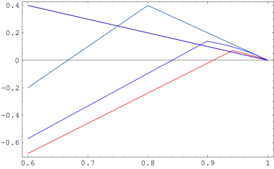
Figure 1: $\Pi_{r}$ when $r=2,\frac{8+2\sqrt{6}}{5},3.$

$\bullet$Step 3: Estimation of $\left\|\omega\right\|_{L^{1}_{t}L^{\widetilde{r}}}$ for every $\widetilde{r}\in[2,r]$ and for some $r\in[2,4[$

Since $\beta>1-\alpha$, there exists a fixed constant $\rho>1$ such that $\frac{\beta}{\rho}>1-\alpha$. From the explicit formula of $\Gamma$ we have for every $\widetilde{r}\in[2,r]$

$$\begin{split}\left\|\omega\right\|_{L^{1}_{t}L^{\widetilde{r}}}&\leq\left\|\Gamma\right\|_{L^{1}_{t}L^{\widetilde{r}}}+\left\|R_{\alpha}\theta\right\|_{L^{1}_{t}B^{0}_{\widetilde{r},1}}\\ &\leq\Phi_{1}(t)+t^{1-\frac{1}{\rho}}\left\|R_{\alpha}\theta\right\|_{\widetilde{L}^{\rho}_{t}B^{0}_{\widetilde{r},1}}.\end{split}$$

By a high-low frequency decomposition and a continuous embedding $B^{\frac{\beta}{\rho}}_{\widetilde{r},\infty}\hookrightarrow B^{1-\alpha}_{\widetilde{r},1}$ we find

$$\begin{split}\left\|R_{\alpha}\theta\right\|_{\widetilde{L}^{\rho}_{t}B^{0}_{\widetilde{r},1}}&\leq\left\|\Delta_{-1}R_{\alpha}\theta\right\|_{\widetilde{L}^{\rho}_{t}B^{0}_{\widetilde{r},1}}+\left\|(Id-\Delta_{-1})\theta\right\|_{\widetilde{L}^{\rho}_{t}B^{1-\alpha}_{\widetilde{r},1}}\\ &\lesssim\left\|\Delta_{-1}\theta\right\|_{L^{\rho}_{t}L^{\widetilde{r}}}+\left\|(Id-\Delta_{-1})\theta\right\|_{\widetilde{L}^{\rho}_{t}B^{\frac{\beta}{\rho}}_{\widetilde{r},\infty}}\\ &\lesssim t^{\frac{1}{\rho}}\left\|\theta^{0}\right\|_{L^{\widetilde{r}}}+\mathrm{sup}_{q\in\mathbb{N}}2^{q\frac{\beta}{\rho}}\left\|\Delta_{q}\theta\right\|_{L^{\rho}_{t}L^{\widetilde{r}}}.\end{split}$$

Inserting this estimate into the previous one and applying Proposition 2.3 we obtain

$$\left\|\omega\right\|_{L^{1}_{t}L^{\widetilde{r}}}\leq\Phi_{1}(t)+Ct^{1-\frac{1}{\rho}}\left\|\omega\right\|_{L^{1}_{t}L^{\widetilde{r}}},$$

where $C$ is an absolute constant depending only on $\widetilde{r},\rho$ and $\left\|\theta^{0}\right\|_{L^{\infty}}$. If $Ct^{1-\frac{1}{\rho}}=\frac{1}{2}$, equivalently, $t=(\frac{1}{2C})^{\rho/(\rho-1)}:=T_{0}$, then for every $t\leq T_{0}$

$$\left\|\omega\right\|_{L^{1}_{t}L^{\widetilde{r}}}\leq\Phi_{1}(t).$$

Furthermore, if we evolve the system (1.1) from the initial data $(u(T_{0}),\theta(T_{0}))$, then using the time translation invariance and the fact that $\left\|\theta(T_{0})\right\|_{L^{\widetilde{r}}}\leq\left\|\theta^{0}\right\|_{L^{\widetilde{r}}}$, we have for every $t\leq T_{0}$

$$\left\|\omega\right\|_{L^{1}_{[T_{0},T_{0}+t]}L^{\widetilde{r}}}\leq\Phi_{1}(T_{0}+t).$$

Iterating like this, we finally get for every $t\in\mathbb{R}^{+}$

$$\left\|\omega\right\|_{L^{1}_{t}L^{\widetilde{r}}}\leq\Phi_{1}(t).$$ (4.6)

$\bullet$Step 4: Estimation of $\left\|\Gamma\right\|_{L^{\sigma}_{t}B^{\frac{2}{r}}_{r,1}}$ for $\sigma\in[1,\frac{\alpha}{1-\alpha+2/r}[$ and $r=r_{0}:=\frac{8+2\sqrt{6}}{5}$

Set $\Gamma_{q}:=\Delta_{q}\Gamma$ for every $q\in\mathbb{N}$. Considering the acting of frequency localization operator $\Delta_{q}$ on the equation (4.2) we get

$$\begin{split}\partial_{t}\Gamma_{q}+u\cdot\nabla\Gamma_{q}+|D|^{\alpha}\Gamma_{q}&=-[\Delta_{q},u\cdot\nabla]\Gamma+\Delta_{q}([R_{\alpha},u\cdot\nabla]\theta)+\Delta_{q}|D|^{\beta}R_{\alpha}\theta\\ &:=f_{q}.\end{split}$$

Since $\Gamma_{q}$ is real-valued, then after multiplying the upper equation by $|\Gamma_{q}|^{r-2}\Gamma_{q}$ and integrating in the spatial variable we obtain

$$\frac{1}{r}\frac{d}{dt}\left\|\Gamma_{q}(t)\right\|_{L^{r}}^{r}+\int_{\mathbb{R}^{2}}|D|^{\alpha}\Gamma_{q}|\Gamma_{q}|^{r-2}\Gamma\mathrm{d}x\leq\left\|\Gamma_{q}(t)\right\|_{L^{r}}^{r-1}\left\|f_{q}(t)\right\|_{L^{r}}.$$

Taking advantaging of the following generalized Bernstein inequality (see [5])

$$\int_{\mathbb{R}^{2}}|D|^{\alpha}\Gamma_{q}|\Gamma_{q}|^{r-2}\Gamma\mathrm{d}x\geq c2^{q\alpha}\left\|\Gamma_{q}\right\|_{L^{r}}^{r},$$

with some positive constant $c$ independent of $q$, we have

$$\frac{1}{r}\frac{d}{dt}\left\|\Gamma_{q}(t)\right\|_{L^{r}}^{r}+c2^{q\alpha}\left\|\Gamma_{q}(t)\right\|_{L^{r}}^{r}\leq\left\|\Gamma_{q}(t)\right\|_{L^{r}}^{r-1}\left\|f_{q}(t)\right\|_{L^{r}}.$$

Thus

$$\left\|\Gamma_{q}(t)\right\|_{L^{r}}\leq e^{-ct2^{q\alpha}}\left\|\Gamma_{q}^{0}\right\|_{L^{r}}+\int_{0}^{t}e^{-c(t-\tau)2^{q\alpha}}\left\|f_{q}(\tau)\right\|_{L^{r}}\mathrm{d}\tau.$$

By taking the $L^{\sigma}([0,t])$ norm and by using the Young inequality we find for every $q\in\mathbb{N}$

$$\begin{split}2^{q\frac{2}{r}}\left\|\Gamma_{q}\right\|_{L^{\sigma}_{t}L^{r}}\lesssim&2^{q(\frac{2}{r}-\frac{\alpha}{\sigma})}\left\|\Gamma_{q}^{0}\right\|_{L^{r}}+2^{q(\frac{2}{r}+1-\alpha-\frac{\alpha}{\sigma})}\int_{0}^{t}2^{q(\alpha-1)}\left\|[\Delta_{q},u\cdot\nabla]\Gamma(\tau)\right\|_{L^{r}}\mathrm{d}\tau\\ &+2^{q(\frac{2}{r}+1-\alpha-\frac{\alpha}{\sigma})}\int_{0}^{t}2^{q(\alpha-1)}\left\|[R_{\alpha},u\cdot\nabla]\theta\right\|_{L^{r}}\mathrm{d}\tau+2^{q(\frac{2}{r}+1+\beta-\alpha-\frac{\alpha}{\sigma})}\left\|\Delta_{q}\theta\right\|_{L^{1}_{t}L^{r}}.\end{split}$$ (4.7)

For the fourth term of the RHS, by using Proposition 2.3, Proposition 4.1 and estimate (4.6) we get for each $q\in\mathbb{N}$

$$\left\|\Delta_{q}\theta\right\|_{L^{1}_{t}L^{r}}\lesssim 2^{-q\beta}(\left\|\theta^{0}\right\|_{L^{r}}+\left\|\theta^{0}\right\|_{L^{\infty}}\left\|\omega\right\|_{L^{1}_{t}L^{r}})\leq 2^{-q\beta}\Phi_{1}(t).$$ (4.8)

For the third term of the RHS, we apply estimate (3.4) with $s=\alpha-1$, Proposition 4.1 and estimate (4.6) to obtain

$$\begin{split}\int_{0}^{t}2^{q(\alpha-1)}\left\|[R_{\alpha},u\cdot\nabla]\theta(\tau)\right\|_{L^{r}}\mathrm{d}\tau&\lesssim\int_{0}^{t}\left\|\nabla u(\tau)\right\|_{L^{r}}\big{(}\left\|\theta(\tau)\right\|_{L^{\infty}}+\left\|\theta(\tau)\right\|_{L^{r}}\big{)}\mathrm{d}\tau\\ &\lesssim\left\|\omega\right\|_{L^{1}_{t}L^{r}}\left\|\theta^{0}\right\|_{L^{\infty}\cap L^{r}}\\ &\leq\Phi_{1}(t).\end{split}$$ (4.9)

For the second term of the RHS, in view of part (1) of Lemma 5.2 and the specific relationship between $u$ and $\theta$ we infer for every $q\in\mathbb{N}$

$$\begin{split}2^{q(\alpha-1)}\left\|[\Delta_{q},u\cdot\nabla]\Gamma(t)\right\|_{L^{r}}&\lesssim(\left\|\nabla u(t)\right\|_{B^{\alpha-1}_{r,\infty}}+\left\|u(t)\right\|_{L^{2}})\left\|\Gamma(t)\right\|_{B^{0}_{\infty,\infty}}\\ &\lesssim(\left\|\Gamma(t)\right\|_{L^{r}}+\left\|\theta(t)\right\|_{L^{r}}+1+t)\left\|\Gamma(t)\right\|_{B^{\frac{2}{r}}_{r,1}}\\ &\leq\Phi_{1}(t)\left\|\Gamma(t)\right\|_{B^{\frac{2}{r}}_{r,1}}.\end{split}$$ (4.10)

To make the sum in the sequel summable, we need $\frac{2}{r}+1-\alpha-\frac{\alpha}{\sigma}<0$, that is,

$$1\leq\sigma<\frac{\alpha}{1-\alpha+2/r},\quad\max\Big{\{}\frac{2+r}{2r},\frac{9r-12}{8r-8}\Big{\}}<\alpha<1,\quad 2\leq r<4.$$

Since for $r\in[2,4[$ the function $\frac{2+r}{2r}$ is monotonously decreasing and $\frac{9r-12}{8r-8}$ monotonously increasing, to obtain the largest scope of $\alpha$, we have to choose $r=r_{0}:=\frac{8+2\sqrt{6}}{5}$ such that $\frac{2+r}{2r}=\frac{9r-12}{8r-8}=\frac{6-\sqrt{6}}{4}$. This leads to

$$(\alpha,\beta)\in\Pi=\Big{]}\frac{6-\sqrt{6}}{4},1\Big{[}\,\times\,\Big{]}1-\alpha,\min\{\frac{7+2\sqrt{6}}{5}\alpha-2,\frac{\alpha(1-\alpha)}{\sqrt{6}-2\alpha},2-2\alpha\}\Big{]}.$$

Let $Q\in\mathbb{N}$ be a number chosen later. By gathering estimates (4.7)-(4.10) together we find

$$\begin{split}\left\|\Gamma\right\|_{\widetilde{L}^{\sigma}_{t}B^{\frac{2}{r}}_{r,1}}&=\sum_{q<Q}2^{q\frac{2}{r}}\left\|\Gamma\right\|_{L^{\sigma}_{t}L^{r}}+\sum_{q\geq Q}2^{q\frac{2}{r}}\left\|\Gamma\right\|_{L^{\sigma}_{t}L^{r}}\\ &\lesssim 2^{Q\frac{2}{r}}\Phi_{1}(t)+2^{-Q(\frac{\alpha}{\sigma}-\frac{2}{r})}\left\|\Gamma^{0}\right\|_{L^{r}}+2^{-Q(\frac{\alpha}{\sigma}+\alpha-1-\frac{2}{r})}(\Phi_{1}(t)+\Phi_{1}(t)\left\|\Gamma\right\|_{L^{1}_{t}B^{\frac{2}{r}}_{r,1}})\\ &\leq\Phi_{1}(t)2^{Q\frac{2}{r}}+2^{-Q(\frac{\alpha}{\sigma}+\alpha-1-\frac{2}{r})}\Phi_{1}(t)\left\|\Gamma\right\|_{\widetilde{L}^{\sigma}_{t}B^{\frac{2}{r}}_{r,1}}.\end{split}$$

We choose $Q$ such that

$$2^{-Q(\frac{\alpha}{\sigma}+\alpha-1-\frac{2}{r})}\Phi_{1}(t)\approx\frac{1}{2},$$

thus we obtain for every $t\in\mathbb{R}^{+}$

$$\left\|\Gamma\right\|_{\widetilde{L}^{\sigma}_{t}B^{\frac{2}{r}}_{r,1}}\leq\Phi_{1}(t).$$ (4.11)

By embedding this immediately leads to

$$\left\|\Gamma\right\|_{\widetilde{L}^{\sigma}_{t}B^{0}_{\infty,1}}\leq\Phi_{1}(t).$$ (4.12)

$\bullet$Step 5: Estimation of $\left\|u\right\|_{L^{1}_{t}B^{1}_{\infty,1}}$

By virtue of estimate (4.12) with $\sigma=1$ and continuous embedding $B^{0}_{\infty,1}\cap L^{2}\hookrightarrow L^{\widetilde{p}}$ for all $\widetilde{p}\in[2,p]$ we get

$$\begin{split}\left\|\omega\right\|_{L^{1}_{t}L^{\widetilde{p}}}&\leq\left\|\Gamma\right\|_{L^{1}_{t}(B^{0}_{\infty,1}\cap L^{2})}+\left\|R_{\alpha}\theta\right\|_{L^{1}_{t}B^{0}_{\widetilde{p},1}}\\ &\leq\Phi_{1}(t)+t^{1-\frac{1}{\rho}}\left\|R_{\alpha}\theta\right\|_{\widetilde{L}^{\rho}_{t}B^{0}_{\widetilde{p},1}}.\end{split}$$

Thus in a similar way as obtaining (4.6), we have for every $\widetilde{p}\in]r_{0},p]$

$$\left\|\omega\right\|_{L^{1}_{t}L^{\widetilde{p}}}\leq\Phi_{1}(t).$$

From Proposition 2.3, we naturally deduce that

$$\sup_{q\in\mathbb{N}}2^{q\beta}\left\|\Delta_{q}\theta\right\|_{L^{1}_{t}L^{\widetilde{p}}}\lesssim\left\|\theta^{0}\right\|_{L^{\widetilde{p}}}+\left\|\theta^{0}\right\|_{L^{\infty}}\left\|\omega\right\|_{L^{1}_{t}L^{\widetilde{p}}}\leq\Phi_{1}(t).$$

Since $\beta>1-\alpha$ and $p>\frac{2}{\alpha+\beta-1}$, there exists a $p_{\alpha}\in]r_{0},p]$ such that $\beta>1-\alpha+\frac{2}{p_{\alpha}}$. Thus

$$\begin{split}\left\|\omega\right\|_{L^{1}_{t}B^{0}_{\infty,1}}&\leq\left\|\Gamma\right\|_{L^{1}_{t}B^{0}_{\infty,1}}+\left\|R_{\alpha}\theta\right\|_{L^{1}_{t}B^{0}_{\infty,1}}\\ &\lesssim\Phi_{1}(t)+\left\|\Delta_{-1}R_{\alpha}\theta\right\|_{L^{1}_{t}L^{\infty}}+\sum_{q\in\mathbb{N}}\left\|\Delta_{q}R_{\alpha}\theta\right\|_{L^{1}_{t}L^{\infty}}\\ &\lesssim\Phi_{1}(t)+t\left\|\theta\right\|_{L^{\infty}_{t}L^{2}}+\sum_{q\in\mathbb{N}}2^{q(1-\alpha+\frac{2}{p_{\alpha}}-\beta)}\sup_{q\in\mathbb{N}}2^{q\beta}\left\|\Delta_{q}\theta\right\|_{L^{1}_{t}L^{p_{\alpha}}}\\ &\leq\Phi_{1}(t).\end{split}$$

This immediately yields

$$\begin{split}\left\|u\right\|_{L^{1}_{t}B^{1}_{\infty,1}}&\lesssim\left\|\Delta_{-1}u\right\|_{L^{1}_{t}L^{\infty}}+\sum_{q\in\mathbb{N}}\left\|\Delta_{q}\nabla u\right\|_{L^{1}_{t}L^{\infty}}\lesssim\left\|u\right\|_{L^{2}}+\left\|\omega\right\|_{L^{1}_{t}B^{0}_{\infty,1}}\\ &\leq\Phi_{1}(t).\end{split}$$ (4.13)

$\bullet$ Step 6: Estimation of $\left\|\theta\right\|_{\widetilde{L}^{\infty}_{t}(H^{1-\alpha}\cap B^{1-\alpha}_{\infty,1})}$ and $\left\|\omega\right\|_{L^{\infty}_{t}L^{p}}$

By Proposition 2.4 and estimate (4.13), we directly obtain

$$\begin{split}\left\|\theta\right\|_{\widetilde{L}^{\infty}_{t}(H^{1-\alpha}\cap B^{1-\alpha}_{\infty,1})}&\lesssim e^{C\left\|\nabla u\right\|_{L^{1}_{t}L^{\infty}}}\left\|\theta^{0}\right\|_{H^{1-\alpha}\cap B^{1-\alpha}_{\infty,1}}\lesssim e^{C\left\|u\right\|_{L^{1}_{t}B^{1}_{\infty,1}}}\\ &\leq\Phi_{2}(t).\end{split}$$ (4.14)

For $p\in]\frac{2}{\alpha+\beta-1},\infty[$, in light of equation (4.2) and Proposition 2.2 we find

$$\left\|\Gamma(t)\right\|_{L^{p}}\leq\left\|\Gamma^{0}\right\|_{L^{p}}+\int_{0}^{t}\left\|[R_{\alpha},u\cdot\nabla]\theta(\tau)\right\|_{L^{p}}\mathrm{d}\tau+\int_{0}^{t}\left\||D|^{\beta}R_{\alpha}\theta(\tau)\right\|_{L^{p}}\mathrm{d}\tau.$$

For the first integral of the RHS, using estimate (3.4) with $s=0$ yields

$$\begin{split}\left\|[R_{\alpha},u\cdot\nabla]\theta(\tau)\right\|_{L^{p}}&\leq\left\|[R_{\alpha},u\cdot\nabla]\theta(\tau)\right\|_{B^{0}_{p,1}}\\ &\lesssim\left\|\nabla u(\tau)\right\|_{L^{p}}(\left\|\theta(\tau)\right\|_{B^{1-\alpha}_{\infty,1}}+\left\|\theta(\tau)\right\|_{L^{p}})\\ &\leq\Phi_{2}(\tau)\left\|\omega(\tau)\right\|_{L^{p}}.\end{split}$$

For the second integral of the RHS, using Proposition 2.4 again we infer

$$\begin{split}\int_{0}^{t}\left\||D|^{\beta}R_{\alpha}\theta(\tau)\right\|_{L^{p}}\mathrm{d}\tau&\lesssim\left\|\theta\right\|_{L^{1}_{t}L^{p}}+\left\|\theta\right\|_{L^{1}_{t}\dot{B}^{1-\alpha+\beta}_{p,1}}\\ &\lesssim\left\|\theta\right\|_{L^{1}_{t}L^{p}}+e^{C\left\|\nabla u\right\|_{L^{1}_{t}L^{\infty}}}\left\|\theta^{0}\right\|_{B^{1-\alpha}_{p,1}}\\ &\leq\Phi_{2}(t).\end{split}$$

Hence

$$\begin{split}\left\|\omega(t)\right\|_{L^{p}}&\leq\left\|\Gamma(t)\right\|_{L^{p}}+\left\|R_{\alpha}\theta(t)\right\|_{L^{p}}\\ &\leq\Phi_{2}(t)+\int_{0}^{t}\Phi_{2}(\tau)\left\|\omega(\tau)\right\|_{L^{p}}\mathrm{d}\tau.\end{split}$$

Gronwall inequality ensures

$$\left\|\omega(t)\right\|_{L^{p}}\leq\Phi_{3}(t).$$ (4.15)

Taking estimates (4.15) and (4.14) into account, we return to Step 4 and further find for every $\sigma\in[1,\frac{\alpha}{1-\alpha+2/p}[$

$$\left\|\Gamma\right\|_{\widetilde{L}^{\sigma}_{t}B^{\frac{2}{p}}_{p,1}}+\left\|u\right\|_{\widetilde{L}^{\sigma}_{t}B^{1}_{\infty,1}}\leq\Phi_{3}(t).$$ (4.16)

This finally ends the proof of Proposition 4.2.

∎

4.2 Uniqueness

We will prove a uniqueness result for the system (1.1) with $(\alpha,\beta)\in\Pi$ in the following space

$$\mathcal{Y}_{T}:=L^{\infty}_{T}H^{1}\cap L^{1}_{T}B^{1}_{\infty,1}\times L^{\infty}_{T}L^{2}\cap L^{1}_{T}B^{1-\alpha}_{\infty,1}.$$

Let ($u_{i},\theta_{i}$)$\in\mathcal{Y}_{T}$ be two solutions of the system 1.1 with initial data ($u^{0}_{i},\theta^{0}_{i}$), $i=1,2$. Set $\delta u:=u_{1}-u_{2}$, $\delta\theta:=\theta_{1}-\theta_{2}$ and $\delta p:=p_{1}-p_{2}$. Then

$$\begin{split}\partial_{t}\delta u+u_{1}\cdot\nabla\delta u+|D|^{\alpha}\delta u+\nabla\delta p\;&=\,-\delta u\cdot\nabla u_{2}+\delta\theta e_{2}\\ \partial_{t}\delta\theta+u_{1}\cdot\nabla\delta\theta+|D|^{\beta}\delta\theta\;&=\,-\delta u\cdot\nabla\theta_{2}\\ (\delta u,\delta\theta)|_{t=0}\;&=\,(\delta u^{0},\delta\theta^{0}).\end{split}$$

To estimate $\delta u$, by means of Lemma 5.3 (and its remark) in the appendix, we choose $\varrho=1$ for term $-\delta u\cdot\nabla u_{2}$ and $\varrho=\infty$ for term $\delta\theta e_{2}$ to get for every $t\in[0,T]$

$$\left\|\delta u(t)\right\|_{B^{0}_{2,\infty}}\lesssim e^{C\left\|u_{1}\right\|_{L^{1}_{t}B^{1}_{\infty,1}}}\Big{(}\left\|\delta u^{0}\right\|_{B^{0}_{2,\infty}}+\int_{0}^{t}\left\|\delta u\cdot\nabla u_{2}(\tau)\right\|_{B^{0}_{2,\infty}}\mathrm{d}\tau+(1+t)\left\|\delta\theta\right\|_{L^{\infty}_{t}B^{-\alpha}_{2,\infty}}\Big{)}.$$ (4.17)

For the integral term of the RHS, point (2) of Lemma 5.2 leads to

$$\left\|\delta u\cdot\nabla u_{2}\right\|_{B^{0}_{2,\infty}}\lesssim\left\|u\right\|_{L^{2}}\left\|u_{2}\right\|_{B^{1}_{\infty,1}}.$$

Using the logarithmic interpolation inequality stated in Lemma 6.10 of [11] we have

$$\left\|\delta u\right\|_{L^{2}}\lesssim\left\|\delta u\right\|_{B^{0}_{2,\infty}}\log(e+\frac{1}{\left\|\delta u\right\|_{B^{0}_{2,\infty}}})\log(e+\left\|\delta u\right\|_{H^{1}}).$$

Thus

$$\left\|\delta u\cdot\nabla u_{2}\right\|_{B^{0}_{2,\infty}}\lesssim\left\|u_{2}\right\|_{B^{1}_{\infty,1}}\log(e+\left\|\delta u\right\|_{H^{1}})\mu(\left\|\delta u\right\|_{B^{0}_{2,\infty}}),$$ (4.18)

where $\mu(x):=x\log(e+\frac{1}{x})$. For the last term of the RHS of (4.17), by virtue of Proposition 2.4, we have for every $t\in[0,T]$

$$\left\|\delta\theta\right\|_{L^{\infty}_{t}B^{-\alpha}_{2,\infty}}\lesssim e^{C\left\|u_{1}\right\|_{L^{1}_{t}B^{1}_{\infty,1}}}\Big{(}\left\|\delta\theta^{0}\right\|_{B^{-\alpha}_{2,\infty}}+\int_{0}^{t}\left\|\delta u\cdot\nabla\theta_{2}(\tau)\right\|_{B^{-\alpha}_{2,\infty}}\mathrm{d}\tau\Big{)}.$$ (4.19)

Taking advantage of Lemma 5.2 and the logarithmic interpolation inequality again we obtain

$$\begin{split}\left\|\delta u\cdot\nabla\theta_{2}\right\|_{B^{-\alpha}_{2,\infty}}&\lesssim\left\|\delta u\right\|_{L^{2}}\left\|\theta_{2}\right\|_{B^{1-\alpha}_{\infty,1}}\\ &\lesssim\left\|\theta_{2}\right\|_{B^{1-\alpha}_{\infty,1}}\log(e+\left\|\delta u\right\|_{H^{1}})\mu(\left\|\delta u\right\|_{B^{0}_{2,\infty}}).\end{split}$$ (4.20)

Denote $Y(t):=\left\|\delta u\right\|_{L^{\infty}_{t}B^{0}_{2,\infty}}+\left\|\delta\theta\right\|_{L^{\infty}_{t}B^{-\alpha}_{2,\infty}}$. Gathering estimates (4.17)-(4.20) together yields

$$Y(t)\leq f(t)\Big{(}Y(0)+\int_{0}^{t}\big{(}\left\|u_{2}(\tau)\right\|_{B^{1}_{\infty,1}}+\left\|\theta_{2}(\tau)\right\|_{B^{1-\alpha}_{\infty,1}}\big{)}\mu(Y(\tau))\mathrm{d}\tau\Big{)},$$

where $f(t)$ is an explicit function which continuously and increasingly depends on $\left\|(u_{i},\theta_{i})\right\|_{\mathcal{Y}_{t}}$ and time $t$. Since

$$\lim_{x\rightarrow 0+}\int_{x}^{1}\frac{1}{\mu(r)}\mathrm{d}r\geq\lim_{x\rightarrow 0+}\log(1+\log\frac{1}{x})=\infty,$$

then the classical Osgood lemma (see Theorem 5.2.1 in [4]) ensures the uniqueness. Moreover, this lemma also shows some quantified estimates as follows

$$Y(0)\leq a(T)\Longrightarrow Y(T)\leq b(T)\big{(}Y(0)\big{)}^{\gamma(T)},$$ (4.21)

where $a,b,\gamma$ are explicit functions depending continuously on $\left\|(u_{i},\theta_{i})\right\|_{\mathcal{Y}_{T}}$ and time $T$.

4.3 Existence

First we smooth the data to get the following approximate system

$$\begin{cases}\partial_{t}u^{(n)}+u^{(n)}\cdot\nabla u^{(n)}+\nabla p^{(n)}+|D|^{\alpha}u^{(n)}=\theta^{(n)}e_{2},\\ \partial_{t}\theta^{(n)}+u^{(n)}\cdot\nabla\theta^{(n)}+|D|^{\beta}\theta^{(n)}=0,\\ \textrm{div}u^{(n)}=0,\\ u^{(n)}|_{t=0}=S_{n}u^{0},\quad\theta^{(n)}|_{t=0}=S_{n}\theta^{0}.\end{cases}$$ (4.22)

Since $S_{n}u^{0},S_{n}\theta^{0}\in H^{s}$ for every $s\in\mathbb{R}$, from the classical theory of quasi-linear hyperbolic systems, we have the local well-posedness of the approximate system. We also have a blowup criterion as follows: if the quantity $\left\|\nabla u^{n}\right\|_{L^{1}_{T}L^{\infty}}$ is finite, the time $T$ can be continued beyond. Then the a priori estimate (4.1) with $\sigma=1$ ensures that the solution $(u^{(n)},\theta^{(n)})$ is globally defined. Moreover, we also have for $\sigma\in[1,\frac{\alpha}{1-\alpha+2/p}[$,

$$\left\|u^{(n)}\right\|_{L^{\sigma}_{T}B^{1}_{\infty,1}}+\left\|u^{(n)}\right\|_{L^{\infty}_{T}(H^{1}\cap\dot{W}^{1,p})}\leq\Phi_{3}(T),$$

$$\left\|\theta^{(n)}\right\|_{L^{\infty}_{T}(H^{1-\alpha}\cap B^{1-\alpha}_{\infty,1})}\leq\Phi_{2}(T).$$

Thus there exists $(u,\theta)$ satisfying the above estimates such that $(u^{(n)},\theta^{(n)})$ weakly converges to $(u,\theta)$ up to the extraction of a subsequence. Furthermore, from (4.21), if

$$d_{n,m}:=\left\|(S_{n}-S_{m})u^{0}\right\|_{B^{0}_{2,\infty}}+\left\|(S_{n}-S_{m})\theta^{0}\right\|_{B^{-\alpha}_{2,\infty}}\leq a(T)$$

then we have

$$\left\|u^{(n)}-u^{(m)}\right\|_{L^{\infty}_{T}B^{0}_{2,\infty}}+\left\|\theta^{(n)}-\theta^{(m)}\right\|_{L^{\infty}_{T}B^{-\alpha}_{2,\infty}}\leq b(T)(d_{n,m})^{\gamma(T)}.$$

This means that $(u^{(n)})$ is of Cauchy and thus it converges strongly to $u$ in $L^{\infty}_{T}B^{0}_{2,\infty}$. By interpolation, we obtain the strong convergence of $u^{(n)}$ to $u$ in $L^{2}([0,T]\times\mathbb{R}^{2})$. Thus $u^{(n)}\otimes u^{(n)}$ strongly converges in $L^{1}([0,T]\times\mathbb{R}^{2})$. But due to that $\theta^{(n)}$ weakly converges to $\theta$ in $L^{2}([0,T]\times\mathbb{R}^{2})$, we have $u^{(n)}\theta^{(n)}$ converges weakly to $u\theta$. It then suffices to pass to the limit in (4.22) and we finally get that $(u,\theta)$ is a solution of our original system (1.1).

5 Appendix: Technical Lemmas

Lemma 5.1.

Let $\gamma\in[2,\infty[$, $s\in]0,1[$, $\alpha\in]\frac{\gamma-4}{\gamma-2},2[$. Then for every smooth function $f$ we have

$$\left\||f|^{\gamma-2}f\right\|_{\dot{H}^{s}}\lesssim\left\|f\right\|_{L^{\frac{2\gamma}{2-\alpha}}}^{\gamma-2}\left\|f\right\|_{\dot{H}^{s+(\frac{n}{2}-\frac{n}{\gamma})(2-\alpha)}}.$$

Proof of Lemma 5.1.

This result is a generalization of Lemma 6.9 in [11], and here we sketch the proof. In fact, by Bernstein inequality, it reduces to prove the following stronger result

$$\left\||f|^{\gamma-2}f\right\|_{\dot{H}^{s}}\lesssim\left\|f\right\|_{L^{\frac{2\gamma}{2-\alpha}}}^{\gamma-2}\left\|f\right\|_{\dot{B}^{s}_{\widetilde{\gamma},2}}.$$

where $\widetilde{\gamma}:=\frac{2\gamma}{\gamma-(\gamma-2)(2-\alpha)}$. For $s\in]0,1[$, we use the characterization of $\dot{H}^{s}$,

$$\left\||f|^{\gamma-2}f\right\|_{\dot{H}^{s}}^{2}\thickapprox\int_{\mathbb{R}^{n}}\frac{\left\||f|^{\gamma-2}f(x+\cdot)-|f|^{\gamma-2}f(\cdot)\right\|^{2}_{L^{2}}}{|x|^{n+2s}}\mathrm{d}x.$$

By using the simple inequality

$$\big{|}|a|^{\gamma-2}a-|b|^{\gamma-2}b\big{|}\lesssim_{\gamma}|a-b|(|a|^{\gamma-2}+|b|^{\gamma-2}),\quad\forall a,b\in\mathbb{R},$$

and Hölder inequality we have for every $\alpha\in]\frac{\gamma-4}{\gamma-2},2[$

$$\begin{split}\left\||f|^{\gamma-2}f(x+\cdot)-|f|^{\gamma-2}f\right\|_{L^{2}}&\lesssim\left\|f(x+\cdot)-f(\cdot)\right\|_{L^{\widetilde{\gamma}}}\left\||f|^{\gamma-2}\right\|_{L^{\frac{2\gamma}{(\gamma-2)(2-\alpha)}}}\\ &\lesssim\left\|f(x+\cdot)-f(\cdot)\right\|_{L^{\widetilde{\gamma}}}\left\|f\right\|_{L^{\frac{2\gamma}{2-\alpha}}}^{\gamma-2}.\end{split}$$

From the characterization of homogeneous Besov space again we get the conclusion.

∎

Next we state some useful estimates in Besov framework.

Lemma 5.2.

Let $u$ be a smooth divergence-free vector field of $\mathbb{R}^{n}$ and $f$ be a smooth scalar function. Then

1. for every $\alpha\in]0,1[$ and $p\in[2,\infty]$

   $$\sup_{q\geq-1}2^{q(\alpha-1)}\left\|[\Delta_{q},u\cdot\nabla]f\right\|_{L^{p}}\lesssim_{\alpha}(\left\|\nabla u\right\|_{B^{\alpha-1}_{p,\infty}}+\left\|u\right\|_{L^{2}})\left\|f\right\|_{B^{0}_{\infty,\infty}}.$$

2. for every $s\in[-1,0]$

   $$\left\|u\cdot\nabla f\right\|_{B^{s}_{2,\infty}}\lesssim\left\|u\right\|_{L^{2}}\left\|f\right\|_{B^{s+1}_{\infty,1}}.$$

Proof of Lemma 5.2.

Note that point (2) is just the one in Lemma 6.10 of [11], thus we only need to prove point (1). From Bony’s decomposition we have

$$\begin{split}&[\Delta_{q},u\cdot\nabla]f\\ =&\sum_{|j-q|\leq 4}[\Delta_{q},S_{j-1}u\cdot\nabla]\Delta_{j}f+\sum_{|j-q|\leq 4}[\Delta_{q},\Delta_{j}u\cdot\nabla]S_{j-1}f+\sum_{j\geq q-4}[\Delta_{q}\partial_{i},\Delta_{j}u^{i}]\widetilde{\Delta}_{j}f\\ :=&\mathrm{I}_{q}+\mathrm{II}_{q}+\mathrm{III}_{q}.\end{split}$$

For $\mathrm{I}_{q}$, since $\Delta_{q}:=h_{q}(\cdot)\star=2^{qn}h(2^{q}\cdot)\star$ with $h\in\mathcal{S}(\mathbb{R}^{n})$, then from (3.1) we get for every $\alpha<1$

$$\begin{split}\left\|\mathrm{I}_{q}\right\|_{L^{p}}&\lesssim\sum_{|j-q|\leq 4}\left\|xh_{q}\right\|_{L^{1}}\left\|\nabla S_{j-1}u\right\|_{L^{p}}2^{j}\left\|\Delta_{j}f\right\|_{L^{\infty}}\\ &\lesssim\left\|f\right\|_{B^{0}_{\infty,\infty}}\left\|xh\right\|_{L^{1}}\sum_{|j-q|\leq 4}2^{j-q}2^{j(1-\alpha)}\sum_{k\leq j-2}2^{(j-k)(\alpha-1)}2^{k(\alpha-1)}\left\|\Delta_{k}\nabla u\right\|_{L^{p}}\\ &\lesssim 2^{q(1-\alpha)}\left\|\nabla u\right\|_{B^{\alpha-1}_{p,\infty}}\left\|f\right\|_{B^{0}_{\infty,\infty}},\end{split}$$

thus

$$\sup_{q\geq-1}2^{q(\alpha-1)}\left\|\mathrm{I}_{q}\right\|_{L^{p}}\lesssim\left\|\nabla u\right\|_{B^{\alpha-1}_{p,\infty}}\left\|f\right\|_{B^{0}_{\infty,\infty}}.$$

For $\mathrm{II}_{q}$, we also use (3.1) to find

$$\begin{split}\left\|\mathrm{II}_{q}\right\|_{L^{p}}&\lesssim\sum_{|j-q|\leq 4}\left\|xh_{q}\right\|_{L^{1}}\left\|\nabla\Delta_{j}u\right\|_{L^{p}}\left\|S_{j-1}\nabla f\right\|_{L^{\infty}}\\ &\lesssim\left\|\nabla u\right\|_{B^{\alpha-1}_{p,\infty}}\sum_{|j-q|\leq 4}2^{-q}2^{j(1-\alpha)}\sum_{k\leq j-2}2^{k}\left\|\Delta_{k}f\right\|_{L^{\infty}}\\ &\lesssim 2^{q(1-\alpha)}\left\|\nabla u\right\|_{B^{\alpha-1}_{p,\infty}}\left\|f\right\|_{B^{0}_{\infty,\infty}},\end{split}$$

thus

$$\sup_{q\geq-1}2^{q(\alpha-1)}\left\|\mathrm{II}_{q}\right\|_{L^{p}}\lesssim\left\|\nabla u\right\|_{B^{\alpha-1}_{p,\infty}}\left\|f\right\|_{B^{0}_{\infty,\infty}}.$$

For $\mathrm{III}_{q}$, we further write

$$\mathrm{III}_{q}=\sum_{j\geq q-4,j\in\mathbb{N}}[\Delta_{q}\partial_{i},\Delta_{j}u^{i}]\widetilde{\Delta}_{j}f+[\Delta_{q}\partial_{i},\Delta_{-1}u^{i}]\widetilde{\Delta}_{-1}f:=\mathrm{III}_{q}^{1}+\mathrm{III}_{q}^{2}.$$

For the first term, by direct computation we have for every $\alpha>0$

$$\begin{split}\left\|\mathrm{III}_{q}^{1}\right\|_{L^{p}}&\leq\sum_{j\geq q-4,j\in\mathbb{N}}\left\|\partial_{i}\Delta_{q}(\Delta_{j}u^{i}\widetilde{\Delta}_{j}f)\right\|_{L^{p}}+\sum_{j\geq q-4,j\in\mathbb{N}}\left\|\Delta_{j}u^{i}\partial_{i}\Delta_{q}\widetilde{\Delta}_{j}f\right\|_{L^{p}}\\ &\lesssim 2^{q(1-\alpha)}\sum_{j\geq q-4,j\in\mathbb{N}}2^{(q-j)\alpha}2^{j(\alpha-1)}\left\|\Delta_{j}\nabla u\right\|_{L^{p}}\left\|\widetilde{\Delta}_{j}f\right\|_{L^{\infty}}\\ &\lesssim_{\alpha}2^{q(1-\alpha)}\left\|\nabla u\right\|_{B^{\alpha-1}_{p,\infty}}\left\|f\right\|_{B^{0}_{\infty,\infty}},\end{split}$$

thus

$$\sup_{q\geq-1}2^{q(\alpha-1)}\left\|\mathrm{III}_{q}^{1}\right\|_{L^{p}}\lesssim_{\alpha}\left\|\nabla u\right\|_{B^{\alpha-1}_{p,\infty}}\left\|f\right\|_{B^{0}_{\infty,\infty}}.$$

For the second term, due to $\mathrm{III}_{q}^{2}=0$ for every $q\geq 3$, we obtain for $p\geq 2$

$$\sup_{q\geq-1}2^{q(\alpha-1)}\left\|\mathrm{III}_{q}^{2}\right\|_{L^{p}}\lesssim\left\|\Delta_{-1}u\right\|_{L^{p}}\left\|\widetilde{\Delta}_{-1}f\right\|_{L^{\infty}}\lesssim\left\|u\right\|_{L^{2}}\left\|f\right\|_{B^{0}_{\infty,\infty}}.$$

This concludes the proof. ∎

The following estimates on the linearized velocity equation is useful in the proof of the uniqueness part.

Lemma 5.3.

Let $s\in]-1,1[$, $\varrho\in[1,\infty]$ and $v$ be a smooth divergence-free vector field of $\mathbb{R}^{n}$. If $u$ be a smooth solution of the linear system

$$\partial_{t}u+v\cdot\nabla u+|D|^{\alpha}u+\nabla p=f,\quad\mathrm{div}u=0.$$

with $\alpha\in[0,2]$ and $u|_{t=0}=u^{0}$, then for each $t\in\mathbb{R}^{+}$ we have

$$\left\|u\right\|_{L^{\infty}_{t}B^{s}_{2,\infty}}\leq Ce^{CV(t)}\bigl{(}\left\|u^{0}\right\|_{B^{s}_{2,\infty}}+(1+t^{1-\frac{1}{\varrho}})\left\|f\right\|_{\widetilde{L}^{\varrho}_{t}B^{s+\frac{\alpha}{\varrho}-\alpha}_{2,\infty}}\bigr{)},$$

where $V(t):=\int_{0}^{t}\left\|\nabla v(\tau)\right\|_{L^{\infty}}\textrm{d}\tau$.

Remark 5.1.

The proof can be done in a similar way as obtaining Proposition 4.3 in [11]. We also note that if $f=f_{1}+f_{2}$, one can choose different $\varrho_{1},\varrho_{2}$ to suit $f_{1},f_{2}$ respectively.

Acknowledgments: The authors would like to thank Prof. T.Hmidi very much for his helpful discussion and suggestions. The authors were partly supported by the NSF of China (No.10725102).

References

[1]H.Abidi, T.Hmidi, On the global wellposedness of the
critical quasi-geostrophic equation, SIAM J. Math. Anal.40, 167-185(2008).
[2] J. T. Beale, T. Kato and A. J. Majda, Remarks on the breakdown of
smooth solutions for the -D Euler equations, Comm. Math.
Phys., 94(1984), 61-66.
[3]D.Chae, Global regularity for the 2-D Boussinesq equations with partial viscous terms, Advances in Math, 203,2 (2006)497-513.
[5]Q.Chen, C.Miao and Z.Zhang, A new Bernstein’s inequality
and the 2D dissipative quasi-geostrophic equation. Comm. Math. Phys. 271. (2007) 821-838
[6]A. Córdoba and D. Córdoba, A maximum principle applied to
the quasi-geostrophic equations. Comm. Math. Phys. 249. (2004) 511-528
[7] R. Danchin. Estimates in Besov spaces for
transport and transport-diffusion equations
with almost Lipschitz coefficients. Rev. Mat.
Iberoamericana. 21 (2005), no.
3,861-886.
[8]R. Danchin and M. Paicu, Le théorème de Leray et le théorèmede Fujita-Kato pour le système de Boussinesq partiellement visqueux.
Bull.Soc.Math.France 136(2008), no.2, 261-309.
[9]T.Hmidi and S.Keraani, Global solutions of the supercritical 2D dissipative quasi-geostrophic equation,
Adv. Math. 214 (2007), 618-638.
[10]T.Hmidi and S.Keraani, On the global well-posedness of the two-dimensional Boussinesq system with a zero diffusivity.
Adv.Differential Equations 12 (2007), no.4,461-480.
[11]T.Hmidi, S.Keraani and F. Rousset, Global well-posedness for a Boussinesq-Navier-Stokes system with critical dissipation. Arxiv,
math.AP/0904,1536.
[12]T.Hmidi, S.Keraani and F. Rousset, Global well-posedness for Euler-Boussinesq system with critical dissipation. Arxiv,
math.AP/0903.3747.
[13]T. Y. Hou and C. Li, Global Well-Posedness of the Viscous Boussinesq Equations, Discrete and Continuous Dynamical Systems, Series A ,12(1),(2005), 1-12.
[14] N. Ju, The maximal principle and the global attrator
for the dissipative 2D quasi-geostrophic equations, Comm. Math. Phys. 255(2005), 161-181.
[15]C.Miao and G.Wu, Global well-posedness of the critical Burgers equation in
critical Besov spaces, J. Differential Equations, 247(2009) 1673-1693
[16]J.Pedlosky, Geophysical fluid dynamics. Springer-Verlag, New York, (1987).