Joint Modelling of Gas and Electricity spot prices

N. Frikha1 , V. Lemaire2
(March 8, 2024)
Abstract

The recent liberalization of the electricity and gas markets has resulted in the growth of energy exchanges and modelling problems. In this paper, we modelize jointly gas and electricity spot prices using a mean-reverting model which fits the correlations structures for the two commodities. The dynamics are based on Ornstein processes with parameterized diffusion coefficients. Moreover, using the empirical distributions of the spot prices, we derive a class of such parameterized diffusions which captures the most salient statistical properties: stationarity, spikes and heavy-tailed distributions.

The associated calibration procedure is based on standard and efficient statistical tools. We calibrate the model on French market for electricity and on UK market for gas, and then we simulate some trajectories which reproduce well the observed prices behavior. Finally, we illustrate the importance of the correlation structure and of the presence of spikes by measuring the risk on a power plant portfolio.

11footnotetext: Laboratoire de Probabilités et Modèles aléatoires, UMR 7599, Université Pierre et Marie Curie, France, e-mail: frikha.noufel@gmail.com22footnotetext: Laboratoire de Probabilités et Modèles aléatoires, UMR 7599, Université Pierre et Marie Curie, France, e-mail: vincent.lemaire@upmc.fr

Keywords: Electricity markets; spot price modelling; ergodic diffusion; stochastic differential equation; saddlepoint

1 Introduction

The recent deregulation of energy markets has led to the development in several countries of market places for energy exchanges. Consequently, understanding and modelling the behavior of energy market is necessary for developing a risk management framework as well as pricing of options. Many derivatives on both electricity and gas spot (and futures) prices are traded. Understanding the correlation structure between both energies is a significant challenge. For instance, spark spread options are commonly traded in energy markets as a way to hedge price differences between electricity and gas prices or are used in order to price projects in energy (see [12] for an introduction). Thus, modelling jointly the evolution of gas and electricity prices is a relevant issue.

Numerous diffusion-type and econometric models have been proposed for electricity and gas spot prices. In energy markets, spot price dynamics are commonly based on Ornstein processes, which are the classical way to model mean-reversion. Geometric models represent the logarithmic prices by a sum of Ornstein processes with different speeds of mean reversion whereas arithmetic models represent the price itself (see for instance [21] for a geometric model). Also, equilibrium models ([2] and [15]) have been investigated in order to reproduce price formation as a balance between supply and demand. The main drawback of such model is that they do not reproduce the autocorrelation structure of a commodity and the cross-correlation structure between commodities. In [13], a markov jump diffusion is investigated for electricity spot prices. Though, it properly represents the spiky behaviour of spot electricity prices, the process reverts to a deterministic mean level whereas it usually reverts to the pre-spike value on data. Moreover applied to electricity and gas spot prices, it does not capture the autocorrelation and cross-correlation struture observed on data.

Another class of spot price dynamics is represented by multifactor models. Several authors (see [14], [4], [9], [20], [22] among others) have investigated this kind of diffusion. The logarithmic prices or the price itself is represented by a sum of Ornstein processes in order to incorporate a mixture of jump variations and “normal” variations. For instance, in [20] the deseasonalized spot price or log-spot price X(t)𝑋𝑡X(t) is given by:

X(t)=Y1(t)+Y2(t)𝑋𝑡subscript𝑌1𝑡subscript𝑌2𝑡X(t)=Y_{1}(t)+Y_{2}(t)

where

dYi(t)=λiYi(t)dt+dLi(t),i=1,2.formulae-sequencedsubscript𝑌𝑖𝑡subscript𝜆𝑖subscript𝑌𝑖𝑡d𝑡dsubscript𝐿𝑖𝑡𝑖12\mbox{d}Y_{i}(t)=-\lambda_{i}Y_{i}(t)\mbox{d}t+\mbox{d}L_{i}(t),\ \ i=1,2.

The Ornstein Uhlenbeck (OU) component Y1subscript𝑌1Y_{1} is responsible for the normal variation and is assumed to be Gaussian, i.e. L1(t)subscript𝐿1𝑡L_{1}(t) is a Brownian motion, whereas Y2subscript𝑌2Y_{2} is the Levy driven OU component responsible for spikes, i.e. L2(t)subscript𝐿2𝑡L_{2}(t) is a jump Lévy process. In this kind of framework, the difficulty is to detect and filter the spikes in order to estimate the jump part. Several methods have been proposed to circumvent this problem (see e.g. [20] and [4]). For instance, [14] presents a similar model for the spot price process that is the exponential of the sum of an Ornstein-Uhlenbeck and an independent mean reverting pure jump process, derives its associated forward curves and finally proposes to calibrate it to the observed forward curve at time t=0𝑡0t=0. In order to calculate premia of call and put options as well as path-dependent options several approximations to the probability density function of the logarithm of the spot price process at maturity are done. In [6], the following spot price dynamics for two energies A𝐴A and B𝐵B are proposed

SA(t)superscript𝑆𝐴𝑡\displaystyle S^{A}(t) =ΛA(t)+i=1mXiA(t)+j=1nYjA(t),absentsuperscriptΛ𝐴𝑡superscriptsubscript𝑖1𝑚superscriptsubscript𝑋𝑖𝐴𝑡superscriptsubscript𝑗1𝑛superscriptsubscript𝑌𝑗𝐴𝑡\displaystyle=\Lambda^{A}(t)+\sum_{i=1}^{m}X_{i}^{A}(t)+\sum_{j=1}^{n}Y_{j}^{A}(t),
SB(t)superscript𝑆𝐵𝑡\displaystyle S^{B}(t) =ΛB(t)+i=1mXiB(t)+j=1nYjB(t),absentsuperscriptΛ𝐵𝑡superscriptsubscript𝑖1𝑚superscriptsubscript𝑋𝑖𝐵𝑡superscriptsubscript𝑗1𝑛superscriptsubscript𝑌𝑗𝐵𝑡\displaystyle=\Lambda^{B}(t)+\sum_{i=1}^{m}X_{i}^{B}(t)+\sum_{j=1}^{n}Y_{j}^{B}(t),

where ΛA(t)superscriptΛ𝐴𝑡\Lambda^{A}(t) and ΛB(t)superscriptΛ𝐵𝑡\Lambda^{B}(t) are seasonal floors, XiAsuperscriptsubscript𝑋𝑖𝐴X_{i}^{A} and XiBsuperscriptsubscript𝑋𝑖𝐵X_{i}^{B} are common OU processes, i.e.formulae-sequence𝑖𝑒i.e. they are driven by the same jump process Lisubscript𝐿𝑖L_{i}. A different approach based on copula is proposed in [5] where the joint evolution of electricity and gas prices is modeled by a bivariate non-Gaussian OU pure jump process with a non-symmetric copula.

In this paper, we propose an alternative class (arithmetic and geometric) of models to reproduce adequately the statistical features of gas and electricity spot prices based on parameterized local volatility processes. The spiky behaviour of both spot prices is captured without introducing jump diffusion processes. More precisely, the deseasonalized (log) prices processes are modelized by the sum of an Ornstein-Uhlenbeck process (which is common for both commodities) and an independent stationary diffusion process. The construction of this stationary diffusion is similar to [7] where diffusion models with linear drift and prespecified marginal distribution are investigated with an application in a different context. The selected parameterized diffusion coefficient allows to capture “cluster of volatility” (e.g. period of high volatility which implies prices spikes).
Moreover, this approach provides a significant advantage over the class of jump diffusion models since the calibration process involves only classical statistical tools like least squares method and maximum likellihood estimations so that it is robust and fast. It allows to reproduce (for the first time to our knowledge) both the auto-correlation and the cross-correlation strutures between two energies. The model was successfully tested on several markets and seems to fit well the statistical features and the marginal distributions of gas and electricity spot prices.

Our results are presented as follows. Section 2 is devoted to the description of the stylised features of gas and electricity spot prices. Then, in Section 3, we briefly recall some important theoretical results on which are based our model. To be more precise, we recall how to construct a mean reverting diffusion process X𝑋X solution of a stochastic differential equation (SDE) with a prespecified continuous invariant density f𝑓f. Such diffusions involves parameterized local volatility processes. In Section 4, we present the model of our choice and focus on the calibration procedure. In the last section, we perform the calibration on the data sets coming from the NBP for the gas spot price and the Powernext market for the electricity spot price. Then, we proceed to the simulation and, finally, analyze the impact of the modelization by measuring the risk of an energy related portfolio using several models. We show that introducing the cross-commodity correlation structure can greatly modify the risk of a portfolio.

2 Stylised features of gas and electricity spot prices

2.1 Seasonality

A first characteristic of gas and electricity (and many commodities) prices is the presence of annual (and possibly multi-time scales) seasonality and a trend (see e.g. [12], [20]). For each commodity, we model the seasonality and the trend component of the logarithmic spot prices with the mean level functions around which spot prices fluctuate

logg(t)𝑔𝑡\displaystyle\log g(t) =ag+bgt+k=1mckgcos(2πtlk)+dkgsin(2πtlk),absentsuperscript𝑎𝑔superscript𝑏𝑔𝑡superscriptsubscript𝑘1𝑚subscriptsuperscript𝑐𝑔𝑘2𝜋𝑡subscript𝑙𝑘subscriptsuperscript𝑑𝑔𝑘2𝜋𝑡subscript𝑙𝑘\displaystyle=a^{g}+b^{g}t+\sum_{k=1}^{m}c^{g}_{k}\cos\left(\frac{2\pi t}{l_{k}}\right)+d^{g}_{k}\sin\left(\frac{2\pi t}{l_{k}}\right),
loge(t)𝑒𝑡\displaystyle\log e(t) =ae+bet+k=1mckecos(2πtlk)+dkesin(2πtlk),absentsuperscript𝑎𝑒superscript𝑏𝑒𝑡superscriptsubscript𝑘1𝑚subscriptsuperscript𝑐𝑒𝑘2𝜋𝑡subscript𝑙𝑘subscriptsuperscript𝑑𝑒𝑘2𝜋𝑡subscript𝑙𝑘\displaystyle=a^{e}+b^{e}t+\sum_{k=1}^{m}c^{e}_{k}\cos\left(\frac{2\pi t}{l_{k}}\right)+d^{e}_{k}\sin\left(\frac{2\pi t}{l_{k}}\right),

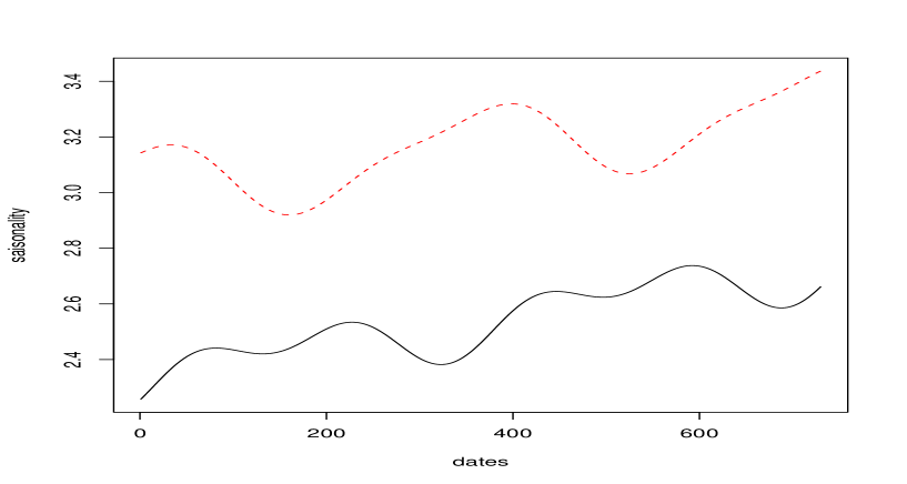
where lk=252/ksubscript𝑙𝑘252𝑘l_{k}=\left\lfloor 252/k\right\rfloor, k=1,,m𝑘1𝑚k=1,\ ...,m, x𝑥\left\lfloor x\right\rfloor denotes the integer part of x𝑥x. For instance, if we choose m=2𝑚2m=2, we only consider a seasonal function over the year and the semester. We assume 252 trading days in a year except for electricity spot price on Powernext which has 365 trading days in a year so that, we have to take into account this particularity in the seasonality function. The coefficients above are estimated using ordinary least squares. The log-seasonality functions are represented with the estimated values for m=2𝑚2m=2 using gas spot price at the NBP and electricity spot price from the Powernext market in Figure 1. All parameters are not significant at the 5% level. We only report and take into account the significant values 111ag=1.53,bg=0.000688,c1g=0.121,d2g=0.0287,c2g=0.00533formulae-sequencesuperscript𝑎𝑔1.53formulae-sequencesuperscript𝑏𝑔0.000688formulae-sequencesuperscriptsubscript𝑐1𝑔0.121formulae-sequencesuperscriptsubscript𝑑2𝑔0.0287superscriptsubscript𝑐2𝑔0.00533a^{g}=1.53,b^{g}=0.000688,c_{1}^{g}=0.121,d_{2}^{g}=0.0287,c_{2}^{g}=0.00533 et ae=3.02,be=0.000405,c1e=0.138,d2e=0.0368.formulae-sequencesuperscript𝑎𝑒3.02formulae-sequencesuperscript𝑏𝑒0.000405formulae-sequencesuperscriptsubscript𝑐1𝑒0.138superscriptsubscript𝑑2𝑒0.0368a^{e}=3.02,b^{e}=0.000405,c_{1}^{e}=0.138,d_{2}^{e}=0.0368.. We checked the seasonality over week, month and quater, but the coefficients were not significant.
Refer to caption
Figure 1: The fitted log-seasonality functions log(g(t))𝑔𝑡\log(g(t)) and log(e(t))𝑒𝑡\log(e(t))

Now we focus our attention on the deseasonalized data Yg(t):=logSg(t)logg(t)assignsuperscript𝑌𝑔𝑡superscript𝑆𝑔𝑡𝑔𝑡Y^{g}(t):=\log S^{g}(t)-\log g(t) and Ye(t):=logSe(t)loge(t)assignsuperscript𝑌𝑒𝑡superscript𝑆𝑒𝑡𝑒𝑡Y^{e}(t):=\log S^{e}(t)-\log e(t) for the specification of the model. A geometric model consists in modelling the stochastic processes Yg(t)superscript𝑌𝑔𝑡Y^{g}(t) and Ye(t)superscript𝑌𝑒𝑡Y^{e}(t) whereas an arithmetic model consists in modelling the stochastic processes eYg(t)superscript𝑒superscript𝑌𝑔𝑡e^{Y^{g}(t)} and eYe(t)superscript𝑒superscript𝑌𝑒𝑡e^{Y^{e}(t)}.

2.2 Spikes and heavy tails

Electricity has very limited storage possibilities. It induces the possibility of spikes in spot prices. Natural gas can be stored but it is often costly, so that it shares the spiky behaviour of spot electricity prices. Gas and electricity markets share this similarity as it can be seen in Figure 2 presenting the electricity spot prices coming from the Powernext market on the left and gas spot prices at the National Balancing Point (NBP) on the right. From a stochastic modelling point of view, spikes are commonly represented by jump diffusions with mean reversion. However (to the best of our knowledge) there is no evidence that it is rather jumps than spikes caused by clusters of volatility for instance.

Refer to caption
Refer to caption
Figure 2: Electricity spot prices on the Powernext market (on the left) and gas spot prices at the NBP (on the right) for the period 14 January 2003 till 20 August 2008.

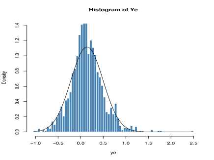
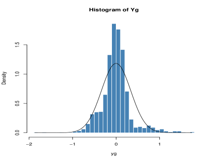
The histograms of Ygsuperscript𝑌𝑔Y^{g} and Yesuperscript𝑌𝑒Y^{e} with the fitted normal density curve is presented in Figure 3. We observe that the two residuals time series Ygsuperscript𝑌𝑔Y^{g} and Yesuperscript𝑌𝑒Y^{e} are far from being normally distributed. The excess of kurtosis of Ygsuperscript𝑌𝑔Y^{g} and Yesuperscript𝑌𝑒Y^{e} are respectively equal to 4.5 and 2.3 meaning that the two distributions are peaked and have heavy tails. The skewness of Ygsuperscript𝑌𝑔Y^{g} and Yesuperscript𝑌𝑒Y^{e} are respectively equal to 0.77 and 0.57 meaning that the two distributions are not symmetric.
Refer to caption
Refer to caption
Figure 3: Histograms of Ygsuperscript𝑌𝑔Y^{g} and Yesuperscript𝑌𝑒Y^{e} with normal density curves.

2.3 Mean reversion and long term dependency

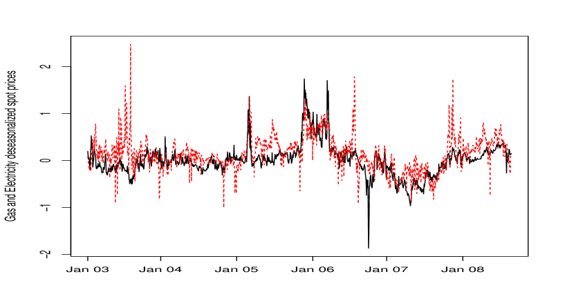
Gas and Electricity spot prices are known to be stationary. This can be tested using an augmented Dickey-Fuller test (ADF) or the Phillips-Perron test. For the UKPX, Powernext electricity spot prices and gas spot prices at the NBP the unit root hypothesis was rejected using both tests. Figure 4 shows that gas and electricity deseasonalized prices are strongly linked by a long term dependency, i.e. it seems that there is a stochastic equilibrium between Yg(t)superscript𝑌𝑔𝑡Y^{g}(t) and Ye(t)superscript𝑌𝑒𝑡Y^{e}(t) from which they cannot deviate for a long time. This long term dependency can be observed on the cross-correlation function.
Refer to caption
Figure 4: The log-deseasonalized gas (normal line) and electricity spot (dashed line) prices

2.4 Auto-correlation and cross-correlation

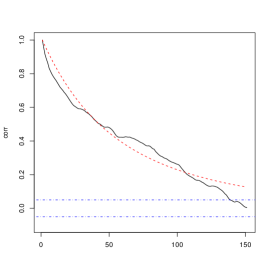
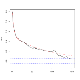
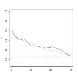
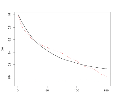
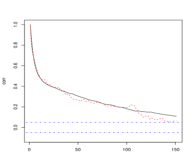
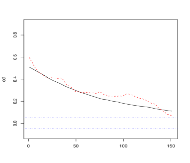
In energy spot price modelling, the auto-correlation functions (ACFs) are often analyzed. The ACFs of both Yg(t)superscript𝑌𝑔𝑡Y^{g}(t) (respectively eYg(t)superscript𝑒superscript𝑌𝑔𝑡e^{Y^{g}(t)}), ρgsuperscript𝜌𝑔\rho^{g}, on one hand Ye(t)superscript𝑌𝑒𝑡Y^{e}(t) (respectively eYe(t)superscript𝑒superscript𝑌𝑒𝑡e^{Y^{e}(t)}), ρesuperscript𝜌𝑒\rho^{e}, on the other hand present both a two-scale (or three-scale at most) decreasing behaviour with one quickly decreasing component and one or two slow decreasing components. The same behaviour is observed on the cross-correlation function (CCF) ρg,esuperscript𝜌𝑔𝑒\rho^{g,e}. This kind of decreasing ACFs and CCF are well explained by sum of decreasing exponentials components, namely for τ>0𝜏0\tau>0:

ρg(τ)superscript𝜌𝑔𝜏\displaystyle\rho^{g}(\tau) =Corr(Yg(t+τ),Yg(t))=ϕ1geλ1gτ+(1ϕ1g)eλ2gτ,absentCorrsuperscript𝑌𝑔𝑡𝜏superscript𝑌𝑔𝑡subscriptsuperscriptitalic-ϕ𝑔1superscript𝑒subscriptsuperscript𝜆𝑔1𝜏1subscriptsuperscriptitalic-ϕ𝑔1superscript𝑒subscriptsuperscript𝜆𝑔2𝜏\displaystyle=\textnormal{Corr}\left(Y^{g}(t+\tau),Y^{g}(t)\right)=\phi^{g}_{1}e^{-\lambda^{g}_{1}\tau}+(1-\phi^{g}_{1})e^{-\lambda^{g}_{2}\tau},
ρe(τ)superscript𝜌𝑒𝜏\displaystyle\rho^{e}(\tau) =Corr(Ye(t+τ),Ye(t))=ϕ1eeλ1eτ+(1ϕ1e)eλ2eτ,absentCorrsuperscript𝑌𝑒𝑡𝜏superscript𝑌𝑒𝑡subscriptsuperscriptitalic-ϕ𝑒1superscript𝑒subscriptsuperscript𝜆𝑒1𝜏1subscriptsuperscriptitalic-ϕ𝑒1superscript𝑒subscriptsuperscript𝜆𝑒2𝜏\displaystyle=\textnormal{Corr}\left(Y^{e}(t+\tau),Y^{e}(t)\right)=\phi^{e}_{1}e^{-\lambda^{e}_{1}\tau}+(1-\phi^{e}_{1})e^{-\lambda^{e}_{2}\tau},
ρg,e(τ)superscript𝜌𝑔𝑒𝜏\displaystyle\rho^{g,e}(\tau) =Corr(Yg(t+τ),Ye(t))=ϕg,eeλg,eτ.absentCorrsuperscript𝑌𝑔𝑡𝜏superscript𝑌𝑒𝑡superscriptitalic-ϕ𝑔𝑒superscript𝑒superscript𝜆𝑔𝑒𝜏\displaystyle=\textnormal{Corr}\left(Y^{g}(t+\tau),Y^{e}(t)\right)=\phi^{g,e}e^{-\lambda^{g,e}\tau}.

For the sake of simplicity in our stochastic modelization, we focused on one type of cross-correlation Corr(Yg(t+τ),Ye(t))Corrsuperscript𝑌𝑔𝑡𝜏superscript𝑌𝑒𝑡\textnormal{Corr}\left(Y^{g}(t+\tau),Y^{e}(t)\right) and we assumed that the cross-correlation is symetric that is Corr(Yg(t+τ),Ye(t))=Corr(Ye(t+τ),Yg(t))Corrsuperscript𝑌𝑔𝑡𝜏superscript𝑌𝑒𝑡Corrsuperscript𝑌𝑒𝑡𝜏superscript𝑌𝑔𝑡\textnormal{Corr}\left(Y^{g}(t+\tau),Y^{e}(t)\right)=\textnormal{Corr}\left(Y^{e}(t+\tau),Y^{g}(t)\right) which is a rather natural approximation. We observed that the slower rates of mean reversion for each commodities are quite similar λ2g=λ2esubscriptsuperscript𝜆𝑔2subscriptsuperscript𝜆𝑒2\lambda^{g}_{2}=\lambda^{e}_{2} and that a rather good approximation is obtained by setting λg,e=λ2g=λ2esuperscript𝜆𝑔𝑒subscriptsuperscript𝜆𝑔2subscriptsuperscript𝜆𝑒2\lambda^{g,e}=\lambda^{g}_{2}=\lambda^{e}_{2}.

Refer to caption
(a) ACF of Ygsuperscript𝑌𝑔Y^{g}
Refer to caption
(b) ACF of Yesuperscript𝑌𝑒Y^{e}
Refer to caption
(c) CCF of (Yg,Ye)superscript𝑌𝑔superscript𝑌𝑒(Y^{g},Y^{e})
Figure 5: Empirical ACF and CCF of deseasonalized gas spot price and electricity spot price

Using a least squares approach, we fitted simulteanously ρg(τ)superscript𝜌𝑔𝜏\rho^{g}(\tau), ρe(τ)superscript𝜌𝑒𝜏\rho^{e}(\tau), ρg,e(τ)superscript𝜌𝑔𝑒𝜏\rho^{g,e}(\tau) (τ=1,,150𝜏1150\tau=1,...,150) to the empirical ACFs and CCF. We assumed that the observed spot prices have reached the stationarity. Both empirical and fitted ACFs222ϕ1g=0.43subscriptsuperscriptitalic-ϕ𝑔10.43\phi^{g}_{1}=0.43, λ1g=7.2subscriptsuperscript𝜆𝑔17.2\lambda^{g}_{1}=7.2, and ϕ1e=0.49subscriptsuperscriptitalic-ϕ𝑒10.49\phi^{e}_{1}=0.49, λ1e=69.4subscriptsuperscript𝜆𝑒169.4\lambda^{e}_{1}=69.4 and CCF333ϕg,e=0.53superscriptitalic-ϕ𝑔𝑒0.53\phi^{g,e}=0.53, λ2g=λ2e=λg,e=2.6subscriptsuperscript𝜆𝑔2subscriptsuperscript𝜆𝑒2superscript𝜆𝑔𝑒2.6\lambda^{g}_{2}=\lambda^{e}_{2}=\lambda^{g,e}=2.6 are plotted in Figure 5.

We can see the separation into a fast speed of mean reversion for gas and electricity spot prices λ1gsubscriptsuperscript𝜆𝑔1\lambda^{g}_{1} and λ1esubscriptsuperscript𝜆𝑒1\lambda^{e}_{1} which corresponds to a correlation dependence of approximately 2 and 30 days probably due to the spikes components whereas the slower speed of mean reversion corresponds to a correlation dependence of 64 days and corresponds to the stochastic equilibrium or the normal variation of gas and electricity spot prices.

3 Theoretical background

In order to modelize heavy tails (and spikes) of stationary spot prices distribution, a natural idea is to consider an ergodic diffusion process like representation of deseasonalized spot prices.

In this section, we briefly recall how to construct a one dimensional process X𝑋X solution of a stochastic differential equation with a prespecified continuous invariant density f𝑓f. Throughout the sequel we assume that f𝑓f is a strictly positive bounded continuous probability density on (l,r)𝑙𝑟(l,r) (and zero outside (l,r)𝑙𝑟(l,r)).

3.1 The general case

Let (Xt)t0subscriptsubscript𝑋𝑡𝑡0{\bigl{(}X_{t}\bigr{)}}_{t\geqslant 0} the diffusion solution of the following stochastic differential equation (SDE)

dXt=b(Xt)dt+σ(Xt)dBt,X0(l,r),formulae-sequencedsubscript𝑋𝑡𝑏subscript𝑋𝑡d𝑡𝜎subscript𝑋𝑡dsubscript𝐵𝑡subscript𝑋0𝑙𝑟\textup{d}X_{t}=b(X_{t})\textup{d}t+\sigma(X_{t})\textup{d}B_{t},\quad X_{0}\in(l,r), (Eb,σsubscript𝐸𝑏𝜎E_{b,\sigma})

where b:(l,r)𝐑:𝑏𝑙𝑟𝐑b:(l,r)\rightarrow\mathbf{R} and σ:(l,r)𝐑:𝜎𝑙𝑟𝐑\sigma:(l,r)\rightarrow\mathbf{R} are locally Lipschitz functions and that σ𝜎\sigma is not degenerate on (l,r)𝑙𝑟(l,r) i.e. x(l,r),σ2(x)>0formulae-sequencefor-all𝑥𝑙𝑟superscript𝜎2𝑥0\forall x\in(l,r),\sigma^{2}(x)>0. We introduce for the diffusion (Xt)t0subscriptsubscript𝑋𝑡𝑡0{\bigl{(}X_{t}\bigr{)}}_{t\geqslant 0}, the scale function p:(l,r)𝐑:𝑝𝑙𝑟𝐑p:(l,r)\rightarrow\mathbf{R} defined for any c(l,r)𝑐𝑙𝑟c\in(l,r) by

x(l,r),p(x)=cxexp(cy2b(z)σ2(z)dz)dy,formulae-sequencefor-all𝑥𝑙𝑟𝑝𝑥superscriptsubscript𝑐𝑥superscriptsubscript𝑐𝑦2𝑏𝑧superscript𝜎2𝑧d𝑧d𝑦\forall x\in(l,r),\quad p(x)=\int_{c}^{x}\exp\left(-\int_{c}^{y}\frac{2b(z)}{\sigma^{2}(z)}\textup{d}z\right)\textup{d}y,

and the speed measure density m:(l,r)𝐑+:𝑚𝑙𝑟superscriptsubscript𝐑m:(l,r)\rightarrow\mathbf{R}_{+}^{*} defined by

x(l,r),m(x)=2p(x)σ2(x)=2σ2(x)exp(cx2b(z)σ2(z)dz).formulae-sequencefor-all𝑥𝑙𝑟𝑚𝑥2superscript𝑝𝑥superscript𝜎2𝑥2superscript𝜎2𝑥superscriptsubscript𝑐𝑥2𝑏𝑧superscript𝜎2𝑧d𝑧\forall x\in(l,r),\quad m(x)=\frac{2}{p^{\prime}(x)\sigma^{2}(x)}=\frac{2}{\sigma^{2}(x)}\exp\left(\int_{c}^{x}\frac{2b(z)}{\sigma^{2}(z)}\textup{d}z\right). (1)

We recall (see e.g. [16, 17]) that the process (p(Xtζ))t0subscript𝑝superscriptsubscript𝑋𝑡𝜁𝑡0\left(p(X_{t}^{\zeta})\right)_{t\geqslant 0} with ζ=inf{t0,Xt=l or Xt=r}𝜁infimumformulae-sequence𝑡0subscript𝑋𝑡𝑙 or subscript𝑋𝑡𝑟\zeta=\inf\left\{t\geqslant 0,X_{t}=l\text{ or }X_{t}=r\right\} is a local martingale if and only if p𝑝p is the scale function (unique up to an affine transformation). Moreover, if the diffusion (Xt)t0subscriptsubscript𝑋𝑡𝑡0{\bigl{(}X_{t}\bigr{)}}_{t\geqslant 0} is positive recurrent, the stationary probability distribution ν𝜈\nu defined on (l,r)𝑙𝑟(l,r) satisfies

ν(dx)=Cm(x)dxwithC=(lrm(x)dx)1.formulae-sequence𝜈d𝑥𝐶𝑚𝑥d𝑥with𝐶superscriptsuperscriptsubscript𝑙𝑟𝑚𝑥d𝑥1\nu(\textup{d}x)=Cm(x)\textup{d}x\quad\text{with}\quad C=\left(\int_{l}^{r}m(x)\textup{d}x\right)^{-1}.

This classical result is the key to construct a one-dimensional ergodic process that fits prescribed stationary probability distribution. For a more general result to construct an inhomogeneous Markov martingale process that has prespecified marginal density we refer to [19].

Proposition 3.1.

Let b:(l,r)𝐑:𝑏𝑙𝑟𝐑b:(l,r)\rightarrow\mathbf{R} be a continuous drift function. Suppose that b𝑏b and f𝑓f satisfy the following conditions

x(l,r),lxb(y)f(y)dy>0,andlrb(y)f(y)dy=0,formulae-sequencefor-all𝑥𝑙𝑟formulae-sequencesuperscriptsubscript𝑙𝑥𝑏𝑦𝑓𝑦d𝑦0andsuperscriptsubscript𝑙𝑟𝑏𝑦𝑓𝑦d𝑦0\quad\forall x\in(l,r),\;\int_{l}^{x}b(y)f(y)\textup{d}y>0,\quad\text{and}\quad\int_{l}^{r}b(y)f(y)\textup{d}y=0, (Bsubscript𝐵\mathcal{H}_{B})

Then there exists a unique continuous diffusion function defined by

x(l,r),σ(x)=2lxb(y)f(y)dyf(x),formulae-sequencefor-all𝑥𝑙𝑟𝜎𝑥2superscriptsubscript𝑙𝑥𝑏𝑦𝑓𝑦d𝑦𝑓𝑥\forall x\in(l,r),\quad\sigma(x)=\sqrt{2\frac{\int_{l}^{x}b(y)f(y)\textup{d}y}{f(x)}},

such that (Eb,σsubscript𝐸𝑏𝜎E_{b,\sigma}) has a unique solution (Xt)t0subscriptsubscript𝑋𝑡𝑡0{\bigl{(}X_{t}\bigr{)}}_{t\geqslant 0}, which is an ergodic diffusion process with stationary distribution ν𝜈\nu satisfying ν(dx)=f(x)dx𝜈d𝑥𝑓𝑥d𝑥\nu(\textup{d}x)=f(x)\textup{d}x.

Further details of the proof outlined below can be found in [7].

Proof.

Let B𝐵B be the function defined by B(x)=lxb(y)f(y)dy𝐵𝑥superscriptsubscript𝑙𝑥𝑏𝑦𝑓𝑦d𝑦B(x)=\int_{l}^{x}b(y)f(y)\textup{d}y. One checks easily that the scale function of (Xt)t0subscriptsubscript𝑋𝑡𝑡0{\bigl{(}X_{t}\bigr{)}}_{t\geqslant 0} satisfies

x(l,r),p(x)=B(c)cx1B(y)dy.formulae-sequencefor-all𝑥𝑙𝑟𝑝𝑥𝐵𝑐superscriptsubscript𝑐𝑥1𝐵𝑦d𝑦\forall x\in(l,r),\quad p(x)=B(c)\int_{c}^{x}\frac{1}{B(y)}\textup{d}y.

One then obtains that limxlp(x)=subscript𝑥𝑙𝑝𝑥\lim_{x\rightarrow l}p(x)=-\infty and limxrp(x)=+subscript𝑥𝑟𝑝𝑥\lim_{x\rightarrow r}p(x)=+\infty.

On the other hand, the speed measure of (Xt)t0subscriptsubscript𝑋𝑡𝑡0{\bigl{(}X_{t}\bigr{)}}_{t\geqslant 0} has density m𝑚m that satisfies

x(l,r),m(x)=f(x)B(x)p(x)=f(x)B(c).formulae-sequencefor-all𝑥𝑙𝑟𝑚𝑥𝑓𝑥𝐵𝑥superscript𝑝𝑥𝑓𝑥𝐵𝑐\forall x\in(l,r),\quad m(x)=\frac{f(x)}{B(x)p^{\prime}(x)}=\frac{f(x)}{B(c)}.

The normalized speed measure density is then equal to the probability density f𝑓f.

To prove existence and uniqueness of the solution (Xt)t0subscriptsubscript𝑋𝑡𝑡0{\bigl{(}X_{t}\bigr{)}}_{t\geqslant 0}, one proves existence and uniqueness of the process (p(Xt))t0subscript𝑝subscript𝑋𝑡𝑡0\left(p(X_{t})\right)_{t\geqslant 0} satisfying a SDE without drift (see [16]). ∎

Corollary 3.2.

Let b:x(l,r)λ(xμ):𝑏𝑥𝑙𝑟maps-to𝜆𝑥𝜇b:x\in(l,r)\mapsto-\lambda(x-\mu) and assume that probability density f𝑓f has expectation μ𝜇\mu and finite variance. Then there exists a unique continuous diffusion function defined by

x(l,r),σ(x)=lx2λ(μy)f(y)dyf(x),formulae-sequencefor-all𝑥𝑙𝑟𝜎𝑥superscriptsubscript𝑙𝑥2𝜆𝜇𝑦𝑓𝑦d𝑦𝑓𝑥\forall x\in(l,r),\quad\sigma(x)=\sqrt{\frac{\int_{l}^{x}2\lambda(\mu-y)f(y)\textup{d}y}{f(x)}},

such that (Eb,σsubscript𝐸𝑏𝜎E_{b,\sigma}) has a unique solution (Xt)t0subscriptsubscript𝑋𝑡𝑡0{\bigl{(}X_{t}\bigr{)}}_{t\geqslant 0}, which is an ergodic diffusion process with stationary distribution ν𝜈\nu satisfying ν(dx)=f(x)dx𝜈d𝑥𝑓𝑥d𝑥\nu(\textup{d}x)=f(x)\textup{d}x, and ACF given by

t,τ0,cor(Xt+τ,Xt)=eλτ.formulae-sequencefor-all𝑡𝜏0corsubscript𝑋𝑡𝜏subscript𝑋𝑡superscript𝑒𝜆𝜏\forall t,\tau\geqslant 0,\quad\operatorname{cor}(X_{t+\tau},X_{t})=e^{-\lambda\tau}.

The squared diffusion coefficients are explicitly known for a large number of commonly used probability diffusions. However, for some specific distributions, it is not possible to obtain a closed form of the diffusion coefficient. An approximation based on saddlepoint technique and the moment generating function (which is generaly known explicitly) is developed in [7].

3.2 Quasi-Saddlepoint approximation

We first recall that saddlepoint approximations are constructed by performing various operations on the moment generating function (MGF) of a random variable (see e.g. [8]). Let X𝑋X be an absolutely continuous random variable with density f𝑓f (with respect to the Lebesgue measure on (l,r)𝑙𝑟(l,r)), moment generating function M(t)𝑀𝑡M(t) and cumulant-generating function κ(t)=logM(t)𝜅𝑡𝑀𝑡\kappa(t)=\log M(t). Then the first-order saddlepoint density approximation to f𝑓f is given by

x(l,r),f^(x)=(2πκ′′(t^x))1/2e(t^xxκ(t^x)),formulae-sequencefor-all𝑥𝑙𝑟^𝑓𝑥superscript2𝜋superscript𝜅′′subscript^𝑡𝑥12superscript𝑒subscript^𝑡𝑥𝑥𝜅subscript^𝑡𝑥\forall x\in(l,r),\quad\hat{f}(x)=\left(2\pi\kappa^{\prime\prime}(\hat{t}_{x})\right)^{-1/2}e^{-\left(\hat{t}_{x}x-\kappa(\hat{t}_{x})\right)},

where t=t^x𝑡subscript^𝑡𝑥t=\hat{t}_{x} is the (unique) solution to the saddlepoint equation κ(t)=xsuperscript𝜅𝑡𝑥\kappa^{\prime}(t)=x, and primes denote derivatives. We assume that the probability density f𝑓f has expectation μ𝜇\mu, i.e. μ=κ(0)𝜇superscript𝜅0\mu=\kappa^{\prime}(0).

Considering the continuous differentiable function t^:xt^x:^𝑡maps-to𝑥subscript^𝑡𝑥\hat{t}:x\mapsto\hat{t}_{x}, an integration by parts gives

0xt^(y)dysuperscriptsubscript0𝑥^𝑡𝑦d𝑦\displaystyle\int_{0}^{x}\hat{t}(y)\textup{d}y =t^(x)x0xt^(y)ydy,absent^𝑡𝑥𝑥superscriptsubscript0𝑥superscript^𝑡𝑦𝑦d𝑦\displaystyle=\hat{t}(x)x-\int_{0}^{x}\hat{t}^{\prime}(y)y\textup{d}y,
=t^(x)x0xdκ(t^(y)),absent^𝑡𝑥𝑥superscriptsubscript0𝑥d𝜅^𝑡𝑦\displaystyle=\hat{t}(x)x-\int_{0}^{x}\textup{d}\kappa(\hat{t}(y)),

since y=κ(t^(y))𝑦superscript𝜅^𝑡𝑦y=\kappa^{\prime}(\hat{t}(y)). The saddlepoint density f^^𝑓\hat{f} writes then

x(l,r),f^(x)=(2πκ′′(t^(x)))1/2exp(0xt(y)dy).formulae-sequencefor-all𝑥𝑙𝑟^𝑓𝑥superscript2𝜋superscript𝜅′′^𝑡𝑥12superscriptsubscript0𝑥𝑡𝑦d𝑦\forall x\in(l,r),\quad\hat{f}(x)=\left(2\pi\kappa^{\prime\prime}(\hat{t}(x))\right)^{-1/2}\exp\left(-\int_{0}^{x}t(y)\textup{d}y\right). (2)

To construct an ergodic process (Xt)t0subscriptsubscript𝑋𝑡𝑡0{\bigl{(}X_{t}\bigr{)}}_{t\geqslant 0} solution of (Eb,σsubscript𝐸𝑏𝜎E_{b,\sigma}) with prespicified stationary density f^^𝑓\hat{f}, the exponential terms that appear in (2) and (1) suggest the relation 2bσ2=t2𝑏superscript𝜎2𝑡\frac{-2b}{\sigma^{2}}=t. This construction is not exact but in [7] is proved that the speed density m𝑚m of X𝑋X is approximately propotional to the saddlepoint density f^^𝑓\hat{f}. To be precise both κ′′(t^(x))superscript𝜅′′^𝑡𝑥\sqrt{\kappa^{\prime\prime}(\hat{t}(x))} and σ2(x)superscript𝜎2𝑥\sigma^{2}(x) are approximately proportional to κ′′(0)+12κ(3)(0)t^(x)superscript𝜅′′012superscript𝜅30^𝑡𝑥\kappa^{\prime\prime}(0)+\frac{1}{2}\kappa^{(3)}(0)\hat{t}(x) near the mean of the distribution. From now this normalized speed density m𝑚m will be called the quasi-saddlepoint density approximation to f𝑓f.

To summarize, if the saddlepoint function t^^𝑡\hat{t} is explicity known and efficiently computed, then we consider the diffusion with drift b𝑏b, such that b>0𝑏0b>0 on (l,μ)𝑙𝜇(l,\mu) and b<0𝑏0b<0 on (μ,r)𝜇𝑟(\mu,r), and with diffusion coefficient

x(l,r),σ(x)=2b(x)t^(x),formulae-sequencefor-all𝑥𝑙𝑟𝜎𝑥2𝑏𝑥^𝑡𝑥\forall x\in(l,r),\quad\sigma(x)=\sqrt{\frac{-2b(x)}{\hat{t}(x)}},

which is ergodic with stationary distribution f~(x)=cσ2(x)e(xt^(x)κ(t^(x)))~𝑓𝑥𝑐superscript𝜎2𝑥superscript𝑒𝑥^𝑡𝑥𝜅^𝑡𝑥\tilde{f}(x)=\frac{c}{\sigma^{2}(x)}e^{-\left(x\hat{t}(x)-\kappa(\hat{t}(x))\right)} (where c𝑐c is a normalizing factor), the quasi-saddlepoint density approximation to f𝑓f (see [7] Theorem 3.1 for more details).

The following example will become useful later when we are going to modelize deseasonalized gas and electricity spot prices.

Example 3.1.

The NIG-distribution The normal-inverse Gaussian (NIG) distribution is a member of the class of generalized hyperbolic distributions (see e.g. [3]). The NIG density is given by

f(x)=αδK1(αδ2+(xl)2)πδ2+(xl)2×eδα2β2+β(xl),x,formulae-sequence𝑓𝑥𝛼𝛿subscript𝐾1𝛼superscript𝛿2superscript𝑥𝑙2𝜋superscript𝛿2superscript𝑥𝑙2superscript𝑒𝛿superscript𝛼2superscript𝛽2𝛽𝑥𝑙𝑥f(x)=\frac{\alpha\delta K_{1}\left(\alpha\sqrt{\delta^{2}+(x-l)^{2}}\right)}{\pi\sqrt{\delta^{2}+(x-l)^{2}}}\times e^{\delta\sqrt{\alpha^{2}-\beta^{2}}+\beta(x-l)},\ \ x\in\mathbb{R},

where β𝐑𝛽𝐑\beta\in\mathbf{R}, α>|β|𝛼𝛽\alpha>|\beta|, δ>0𝛿0\delta>0, l𝑙l\in\mathbb{R} and K1subscript𝐾1K_{1} is the the modified Bessel function of third order and index 111. Note that if XNIG(α,β,δ,l)similar-to𝑋NIG𝛼𝛽𝛿𝑙X\sim\textup{NIG}\left(\alpha,\beta,\delta,l\right) then its two first moments are

𝐄[X]=l+δβα2β2etvar(X)=δα2(α2β2)32.formulae-sequence𝐄delimited-[]𝑋𝑙𝛿𝛽superscript𝛼2superscript𝛽2etvar𝑋𝛿superscript𝛼2superscriptsuperscript𝛼2superscript𝛽232\mathbf{E}\left[X\right]=l+\frac{\delta\beta}{\sqrt{\alpha^{2}-\beta^{2}}}\quad\text{et}\quad\operatorname{var}(X)=\frac{\delta\alpha^{2}}{(\alpha^{2}-\beta^{2})^{\frac{3}{2}}}.

The two parameters δ𝛿\delta and l𝑙l determine respectivelly the scale and the location of the law, and the two parameters α𝛼\alpha and β𝛽\beta determine the shape: α𝛼\alpha being responsible for the tail heavyness and β𝛽\beta for the skewness (asymmetry).

The cumulant-generating function κ𝜅\kappa of the NIG distribution is defined for all t𝑡t such that |β+t|<α𝛽𝑡𝛼|\beta+t|<\alpha by

κ(t)=lt+δ(α2β2α2(β+t)2),𝜅𝑡𝑙𝑡𝛿superscript𝛼2superscript𝛽2superscript𝛼2superscript𝛽𝑡2\kappa(t)=lt+\delta\left(\sqrt{\alpha^{2}-\beta^{2}}-\sqrt{\alpha^{2}-(\beta+t)^{2}}\right),

and the saddlepoint function is defined by

x𝐑,t^(x)=α(xl)δ2+(xl)2β.formulae-sequencefor-all𝑥𝐑^𝑡𝑥𝛼𝑥𝑙superscript𝛿2superscript𝑥𝑙2𝛽\forall x\in\mathbf{R},\quad\hat{t}(x)=\frac{\alpha\left(x-l\right)}{\sqrt{\delta^{2}+(x-l)^{2}}}-\beta.

In order to have an Ornstein process solution of (Eb,σsubscript𝐸𝑏𝜎E_{b,\sigma}) with stationary density the quasi-saddlepoint density approximation f~~𝑓\tilde{f} to f𝑓f, we consider the following drift and diffusion functions

x𝐑,b(x)=λ(xμ)andσ2(x)=2λδ2+(xl)2(xμ)α(xl)βδ2+(xl)2,formulae-sequencefor-all𝑥𝐑formulae-sequence𝑏𝑥𝜆𝑥𝜇andsuperscript𝜎2𝑥2𝜆superscript𝛿2superscript𝑥𝑙2𝑥𝜇𝛼𝑥𝑙𝛽superscript𝛿2superscript𝑥𝑙2\forall x\in\mathbf{R},\quad b(x)=-\lambda\left(x-\mu\right)\quad\text{and}\quad\sigma^{2}(x)=\frac{2\lambda\sqrt{\delta^{2}+(x-l)^{2}}\left(x-\mu\right)}{\alpha\left(x-l\right)-\beta\sqrt{\delta^{2}+(x-l)^{2}}}, (3)

with μ=l+δβα2β2𝜇𝑙𝛿𝛽superscript𝛼2superscript𝛽2\mu=l+\frac{\delta\beta}{\sqrt{\alpha^{2}-\beta^{2}}}.

4 Cross-commodity multi-factor model

In this section, we present two class of cross-commodity multi factor models: the geometric and the arithmetic class. Those two class are commonly used in stochastic modelling of commodity prices. The first one ensures the positivity of simulated spot prices. However, when dealing with forward contracts which have a delivery period or options pricing, the second one is analytically more tractable. Both class of models are based on stationary diffusion-type models analyzed in [7].

4.1 Proposed modelization

In this section, we propose an alternative model which captures the stylized features described in Section 2 without introducing jump diffusions. Sums of this kind of diffusions can fit the multi-scale ACFs and the CCF obtained for the deseasonalized gas and electricity spot prices.

In order to represent the ACFs and CCF of gas and electricity deseasonalized spot prices, we are led to introduce stochastic processes that are sums of diffusions defined by (Eb,σ)subscript𝐸𝑏𝜎(E_{b,\sigma}). To be more precise, we focus on the following two factor modelization for the deseasonalized log spot prices Ygsuperscript𝑌𝑔Y^{g} and Yesuperscript𝑌𝑒Y^{e}

Ytg=Xtg+Zt, and Yte=Xte+Zt,formulae-sequencesubscriptsuperscript𝑌𝑔𝑡subscriptsuperscript𝑋𝑔𝑡subscript𝑍𝑡 and subscriptsuperscript𝑌𝑒𝑡subscriptsuperscript𝑋𝑒𝑡subscript𝑍𝑡Y^{g}_{t}=X^{g}_{t}+Z_{t},\ \ \mbox{ and }\ \ Y^{e}_{t}=X^{e}_{t}+Z_{t}, (4)

where (Zt)t0subscriptsubscript𝑍𝑡𝑡0{\bigl{(}Z_{t}\bigr{)}}_{t\geqslant 0}, (Xtg)t0subscriptsubscriptsuperscript𝑋𝑔𝑡𝑡0{\bigl{(}X^{g}_{t}\bigr{)}}_{t\geqslant 0} and (Xte)t0subscriptsubscriptsuperscript𝑋𝑒𝑡𝑡0{\bigl{(}X^{e}_{t}\bigr{)}}_{t\geqslant 0} are mutually independant processes defined as following:

  • the process (Zt)t0subscriptsubscript𝑍𝑡𝑡0{\bigl{(}Z_{t}\bigr{)}}_{t\geqslant 0} accounts for the stochastic equilibrium between both commodities with a slow rate of mean reversion λz=λ2g=λ2esubscript𝜆𝑧superscriptsubscript𝜆2𝑔superscriptsubscript𝜆2𝑒\lambda_{z}=\lambda_{2}^{g}=\lambda_{2}^{e}. Thus, it represents the normal variation and will be defined by an Ornstein-Uhlenbeck process

    dZt=λzZtdt+σzdWtz,dsubscript𝑍𝑡subscript𝜆𝑧subscript𝑍𝑡d𝑡subscript𝜎𝑧dsubscriptsuperscript𝑊𝑧𝑡\textup{d}Z_{t}=-\lambda_{z}Z_{t}\textup{d}t+\sigma_{z}\textup{d}W^{z}_{t}, (5)

    with λz>0subscript𝜆𝑧0\lambda_{z}>0 and σz𝐑subscript𝜎𝑧𝐑\sigma_{z}\in\mathbf{R}. Note that Z𝑍Z is ergodic with the Gaussian invariant probability 𝒩(0,σz2/2λz)𝒩0superscriptsubscript𝜎𝑧22subscript𝜆𝑧\mathcal{N}\left(0,\sigma_{z}^{2}/2\lambda_{z}\right).

  • the processes (Xtg)t0subscriptsubscriptsuperscript𝑋𝑔𝑡𝑡0{\bigl{(}X^{g}_{t}\bigr{)}}_{t\geqslant 0} and (Xte)t0subscriptsubscriptsuperscript𝑋𝑒𝑡𝑡0{\bigl{(}X^{e}_{t}\bigr{)}}_{t\geqslant 0} represent the spikes component for each commodity. We modelize them by general Ornstein processes with high rate of mean reversion λg=λ1g>0subscript𝜆𝑔superscriptsubscript𝜆1𝑔0\lambda_{g}=\lambda_{1}^{g}>0 and λe=λ2e>0subscript𝜆𝑒superscriptsubscript𝜆2𝑒0\lambda_{e}=\lambda_{2}^{e}>0, namely

    dXtj=λj(Xtjμj)dt+σj(Xtj;θj)dWtj,j=g,e,formulae-sequencedsubscriptsuperscript𝑋𝑗𝑡subscript𝜆𝑗subscriptsuperscript𝑋𝑗𝑡subscript𝜇𝑗d𝑡subscript𝜎𝑗subscriptsuperscript𝑋𝑗𝑡subscript𝜃𝑗dsubscriptsuperscript𝑊𝑗𝑡𝑗𝑔𝑒\textup{d}X^{j}_{t}=-\lambda_{j}\left(X^{j}_{t}-\mu_{j}\right)\textup{d}t+\sigma_{j}(X^{j}_{t};\theta_{j})\textup{d}W^{j}_{t},\ j=g,e, (6)

    where σjsubscript𝜎𝑗\sigma_{j} is a parametric diffusion function such that (Xtg)t0subscriptsubscriptsuperscript𝑋𝑔𝑡𝑡0{\bigl{(}X^{g}_{t}\bigr{)}}_{t\geqslant 0} is an ergodic diffusion with invariant probability fj(.,θj)f^{j}(.,\theta_{j}).

Remark 4.1.

The following contruction can be extended to a more general multi-factor model. We can consider m𝑚m general Ornstein processes and p𝑝p Ornstein-Uhlenbeck processes so that

Yg(t)superscript𝑌𝑔𝑡\displaystyle Y^{g}(t) =i=1mXig(t)+j=1pZj(t),absentsuperscriptsubscript𝑖1𝑚subscriptsuperscript𝑋𝑔𝑖𝑡superscriptsubscript𝑗1𝑝subscript𝑍𝑗𝑡\displaystyle=\sum_{i=1}^{m}X^{g}_{i}(t)+\sum_{j=1}^{p}Z_{j}(t),
Ye(t)superscript𝑌𝑒𝑡\displaystyle Y^{e}(t) =i=1mXie(t)+j=1pZj(t),absentsuperscriptsubscript𝑖1𝑚subscriptsuperscript𝑋𝑒𝑖𝑡superscriptsubscript𝑗1𝑝subscript𝑍𝑗𝑡\displaystyle=\sum_{i=1}^{m}X^{e}_{i}(t)+\sum_{j=1}^{p}Z_{j}(t),

where all processes are assumed to be mutually independent, i.e. driven by independent Wiener processes. We already observed that a two-factor model (m=1𝑚1m=1 and p=1𝑝1p=1) fits the ACFs and CCF well.

Proposition 4.1 (The correlation structures).

Let Yg,Yesuperscript𝑌𝑔superscript𝑌𝑒Y^{g},\ Y^{e} be the processes defined in (4). Then, the ACFs of Ygsuperscript𝑌𝑔Y^{g} and Yesuperscript𝑌𝑒Y^{e} with lag τ>0𝜏0\tau>0 are given by

ρg(τ)=cor(Yt+τg,Ytg)superscript𝜌𝑔𝜏corsubscriptsuperscript𝑌𝑔𝑡𝜏subscriptsuperscript𝑌𝑔𝑡\displaystyle\rho^{g}(\tau)=\operatorname{cor}\left(Y^{g}_{t+\tau},Y^{g}_{t}\right) =ϕgeλgτ+(1ϕg)eλzτ,absentsubscriptitalic-ϕ𝑔superscript𝑒subscript𝜆𝑔𝜏1subscriptitalic-ϕ𝑔superscript𝑒subscript𝜆𝑧𝜏\displaystyle=\phi_{g}e^{-\lambda_{g}\tau}+(1-\phi_{g})e^{-\lambda_{z}\tau},
ρe(τ)=cor(Yt+τe,Yte)superscript𝜌𝑒𝜏corsubscriptsuperscript𝑌𝑒𝑡𝜏subscriptsuperscript𝑌𝑒𝑡\displaystyle\rho^{e}(\tau)=\operatorname{cor}\left(Y^{e}_{t+\tau},Y^{e}_{t}\right) =ϕeeλeτ+(1ϕe)eλzτ,absentsubscriptitalic-ϕ𝑒superscript𝑒subscript𝜆𝑒𝜏1subscriptitalic-ϕ𝑒superscript𝑒subscript𝜆𝑧𝜏\displaystyle=\phi_{e}e^{-\lambda_{e}\tau}+(1-\phi_{e})e^{-\lambda_{z}\tau},

where

ϕg=Var(Xg(t))Var(Yg(t)), and ϕe=Var(Xe(t))Var(Ye(t)).formulae-sequencesubscriptitalic-ϕ𝑔Varsuperscript𝑋𝑔𝑡Varsuperscript𝑌𝑔𝑡 and subscriptitalic-ϕ𝑒Varsuperscript𝑋𝑒𝑡Varsuperscript𝑌𝑒𝑡\phi_{g}=\frac{\textnormal{Var}\left(X^{g}(t)\right)}{\textnormal{Var}\left(Y^{g}(t)\right)},\ \ \mbox{ and }\ \ \phi_{e}=\frac{\textnormal{Var}\left(X^{e}(t)\right)}{\textnormal{Var}\left(Y^{e}(t)\right)}.

The CCF with lag τ>0𝜏0\tau>0 is given by

ρg,e(τ):=cor(Yt+τg,Yte)=ϕg,eeλzτ,assignsuperscript𝜌𝑔𝑒𝜏corsubscriptsuperscript𝑌𝑔𝑡𝜏subscriptsuperscript𝑌𝑒𝑡subscriptitalic-ϕ𝑔𝑒superscript𝑒subscript𝜆𝑧𝜏\rho^{g,e}(\tau):=\operatorname{cor}\left(Y^{g}_{t+\tau},Y^{e}_{t}\right)=\phi_{g,e}\ e^{-\lambda_{z}\tau},

with, ϕg,e=Var(Z(t))Var(Yg(t))Var(Ye(t)).subscriptitalic-ϕ𝑔𝑒Var𝑍𝑡Varsuperscript𝑌𝑔𝑡Varsuperscript𝑌𝑒𝑡\phi_{g,e}=\frac{\textnormal{Var}\left(Z(t)\right)}{\sqrt{\textnormal{Var}\left(Y^{g}(t)\right)\textnormal{Var}\left(Y^{e}(t)\right)}}.

From the definition of ϕg,esubscriptitalic-ϕ𝑔𝑒\phi_{g,e}, we find that σz2=2λzϕg,eVar(Yg(t))Var(Ye(t))superscriptsubscript𝜎𝑧22subscript𝜆𝑧subscriptitalic-ϕ𝑔𝑒Varsuperscript𝑌𝑔𝑡Varsuperscript𝑌𝑒𝑡\sigma_{z}^{2}=2\lambda_{z}\phi_{g,e}\sqrt{\textnormal{Var}\left(Y^{g}(t)\right)\textnormal{Var}\left(Y^{e}(t)\right)}, where the last term is the product of the two stationary variance of the two processes. Consequently, one can easily derive σzsubscript𝜎𝑧\sigma_{z} from the ACFs and CCF calibration.

4.2 Calibration

We propose a three-step calibration procedure for the model described above.

Step 1: Deseasonalizing spot prices

We fit the seasonality functions g(t)𝑔𝑡g(t) and e(t)𝑒𝑡e(t) defined in section 2.1 to the logarithmic spot prices. The parameters of the functions are estimated using the least squares approach. Now, we focus on the deseasonalized spot prices Ygsuperscript𝑌𝑔Y^{g} and Yesuperscript𝑌𝑒Y^{e} defined by

Yg(t)=log(Sg(t))log(g(t)) and Ye(t)=log(Se(t))log(e(t)).formulae-sequencesuperscript𝑌𝑔𝑡superscript𝑆𝑔𝑡𝑔𝑡 and superscript𝑌𝑒𝑡superscript𝑆𝑒𝑡𝑒𝑡Y^{g}(t)=\log\left(S^{g}(t)\right)-\log\left(g(t)\right)\ \ \mbox{ and }\ \ Y^{e}(t)=\log\left(S^{e}(t)\right)-\log\left(e(t)\right).

One can consider the deseasonalized spot prices eYg(t)superscript𝑒superscript𝑌𝑔𝑡e^{Y^{g}(t)} and eYe(t)superscript𝑒superscript𝑌𝑒𝑡e^{Y^{e}(t)} instead of this geometric approach.

Step 2: ACFs and CCF

The least squares method consists in fitting the empirical ACFs ρg(τ)superscript𝜌𝑔𝜏\rho^{g}(\tau), ρe(τ)superscript𝜌𝑒𝜏\rho^{e}(\tau) and CCF ρg,e(τ)superscript𝜌𝑔𝑒𝜏\rho^{g,e}(\tau) defined in section 2.4 to the empirical ones (ρ~g(τ))τ=1,,lsubscriptsuperscript~𝜌𝑔𝜏𝜏1𝑙\left(\tilde{\rho}^{g}(\tau)\right)_{\tau=1,...,l}, (ρ~e(τ))τ=1,,lsubscriptsuperscript~𝜌𝑒𝜏𝜏1𝑙\left(\tilde{\rho}^{e}(\tau)\right)_{\tau=1,...,l}, (ρ~g,e(τ))τ=1,,lsubscriptsuperscript~𝜌𝑔𝑒𝜏𝜏1𝑙\left(\tilde{\rho}^{g,e}(\tau)\right)_{\tau=1,...,l} in order to derive the three speeds of mean reversion λ1gsuperscriptsubscript𝜆1𝑔\lambda_{1}^{g}, λ1esuperscriptsubscript𝜆1𝑒\lambda_{1}^{e}, λzsubscript𝜆𝑧\lambda_{z} with the diffusion coefficient σzsubscript𝜎𝑧\sigma_{z} of the stochastic equilibrium process Z𝑍Z. This can be done by minimizing the sum of squared differences, namely

argminλg,λe,λz,σzτ=1l((ρg(τ)ρ~g(τ))2+(ρe(τ)ρ~e(τ))2+(ρg,e(τ)ρ~g,e(τ))2).subscriptargminsubscript𝜆𝑔subscript𝜆𝑒subscript𝜆𝑧subscript𝜎𝑧superscriptsubscript𝜏1𝑙superscriptsuperscript𝜌𝑔𝜏superscript~𝜌𝑔𝜏2superscriptsuperscript𝜌𝑒𝜏superscript~𝜌𝑒𝜏2superscriptsuperscript𝜌𝑔𝑒𝜏superscript~𝜌𝑔𝑒𝜏2\operatorname*{arg\,min}_{\lambda_{g},\lambda_{e},\lambda_{z},\sigma_{z}}\sum_{\tau=1}^{l}\left(\left(\rho^{g}(\tau)-\tilde{\rho}^{g}(\tau)\right)^{2}+\left(\rho^{e}(\tau)-\tilde{\rho}^{e}(\tau)\right)^{2}+\left(\rho^{g,e}(\tau)-\tilde{\rho}^{g,e}(\tau)\right)^{2}\right).

Stability tests showed that the estimates are robust with respect to small changes in the initial values of the parameters.

Step 3: Estimating the parameters of the spikes component

The final step consists in statiscally estimating the parameters θgsubscript𝜃𝑔\theta_{g} of the invariant density fg(.,θg)f^{g}(.,\theta_{g}) of the process Xgsuperscript𝑋𝑔X^{g} and the parameters θesubscript𝜃𝑒\theta_{e} of the invariant density fe(.,θe)f^{e}(.,\theta_{e}) of the process Xesuperscript𝑋𝑒X^{e}. For instance, if one decide to choose the quasi-saddlepoint approximation to the NIG density for fgsuperscript𝑓𝑔f^{g} and fesuperscript𝑓𝑒f^{e}, there will be four parameters to fit for each density. The model proposed is a sum of diffusion processes and hence is not Markovian. Thus, the likelihood cannot be written down explicitly. To overcome this problem, we use the maximum likelihood estimation of order m𝑚m (m=0𝑚0m=0 or m=1𝑚1m=1 in our case) method for stationary processes introduced in [1]. Strong consistency and a Central Limit Theorem are proved for such estimates. It consists in approximating the log-likelihood of the serie (ykj)1knsubscriptsubscriptsuperscript𝑦𝑗𝑘1𝑘𝑛(y^{j}_{k})_{1\leq k\leq n} (j=g,e𝑗𝑔𝑒j=g,\ e), where n𝑛n is the number of sample points, by a sum whose generic term is the density function of Ykjsubscriptsuperscript𝑌𝑗𝑘Y^{j}_{k} conditional on the m𝑚m most recent observations, for some m0𝑚0m\geq 0, namely,

mj(θ)=k=1nlog(hj(ykj|ykj,m;θj)),superscriptsubscript𝑚𝑗𝜃superscriptsubscript𝑘1𝑛superscript𝑗conditionalsubscriptsuperscript𝑦𝑗𝑘subscriptsuperscript𝑦𝑗𝑚𝑘subscript𝜃𝑗\ell_{m}^{j}(\theta)=\sum_{k=1}^{n}\log\left(h^{j}(y^{j}_{k}\ |\ y^{j,m}_{k};\theta_{j})\right), (7)

where ykj,m:=(ykmj,,yk1j)assignsubscriptsuperscript𝑦𝑗𝑚𝑘subscriptsuperscript𝑦𝑗𝑘𝑚subscriptsuperscript𝑦𝑗𝑘1y^{j,m}_{k}:=(y^{j}_{k-m},\cdots,y^{j}_{k-1}) and hj(.|ykj,m;θj)h^{j}(.\ |\ y^{j,m}_{k};\theta_{j}) is the conditional probability density function of Ykjsubscriptsuperscript𝑌𝑗𝑘Y^{j}_{k} given Ykj,m=ykj,msubscriptsuperscript𝑌𝑗𝑚𝑘subscriptsuperscript𝑦𝑗𝑚𝑘Y^{j,m}_{k}=y^{j,m}_{k} for the parameters θjsubscript𝜃𝑗\theta_{j}. Note that if m=0𝑚0m=0, there is no conditioning and hjsuperscript𝑗h^{j} is simply the marginal density of Ykjsubscriptsuperscript𝑌𝑗𝑘Y^{j}_{k}, k=1,,n𝑘1𝑛k=1,\cdots,n, which is the convolution of Zksubscript𝑍𝑘Z_{k} and Xkjsubscriptsuperscript𝑋𝑗𝑘X^{j}_{k}. We suppose that (Xkj)1knsubscriptsubscriptsuperscript𝑋𝑗𝑘1𝑘𝑛(X^{j}_{k})_{1\leq k\leq n} (resp. (Zk)1knsubscriptsubscript𝑍𝑘1𝑘𝑛(Z_{k})_{1\leq k\leq n}) is ergodic with stationary distribution fj(.;θj)f^{j}(.;\theta_{j}) (resp. with Gaussian invariant probability 𝒩(0,σZ~2:=σz2/2λz)𝒩assign0superscript~subscript𝜎𝑍2superscriptsubscript𝜎𝑧22subscript𝜆𝑧\mathcal{N}\left(0,\tilde{\sigma_{Z}}^{2}:=\sigma_{z}^{2}/2\lambda_{z}\right)) so that the conditional probability density function is given by

hj(ykj;θj)=+fj(ykjσZλZu;θj)eu2πdu,j=g,e.formulae-sequencesuperscript𝑗subscriptsuperscript𝑦𝑗𝑘subscript𝜃𝑗superscriptsubscriptsuperscript𝑓𝑗subscriptsuperscript𝑦𝑗𝑘subscript𝜎𝑍subscript𝜆𝑍𝑢subscript𝜃𝑗superscript𝑒superscript𝑢2𝜋d𝑢𝑗𝑔𝑒h^{j}(y^{j}_{k};\theta_{j})=\int_{-\infty}^{+\infty}f^{j}\left(y^{j}_{k}-\frac{\sigma_{Z}}{\sqrt{\lambda_{Z}}}u;\theta_{j}\right)\frac{e^{-u^{2}}}{\sqrt{\pi}}\textup{d}u,\quad j=g,e. (8)

Note that it corresponds to the case of (Ykj)1knsubscriptsubscriptsuperscript𝑌𝑗𝑘1𝑘𝑛(Y^{j}_{k})_{1\leq k\leq n} is independent and identically distributed random variables having the distribution of the stationary distribution of Yjsuperscript𝑌𝑗Y^{j}.

Numerically, the above integral can be approximated using a Gauss-Hermite quadrature method, namely

hj(ykj;θj)1πk=1nfj(xσZλZuk;θj)wk,j=g,e,formulae-sequencesuperscript𝑗subscriptsuperscript𝑦𝑗𝑘subscript𝜃𝑗1𝜋superscriptsubscript𝑘1𝑛superscript𝑓𝑗𝑥subscript𝜎𝑍subscript𝜆𝑍subscript𝑢𝑘subscript𝜃𝑗subscript𝑤𝑘𝑗𝑔𝑒h^{j}(y^{j}_{k};\theta_{j})\approx\frac{1}{\sqrt{\pi}}\sum_{k=1}^{n}f^{j}\left(x-\frac{\sigma_{Z}}{\sqrt{\lambda_{Z}}}u_{k};\theta_{j}\right)w_{k},\quad j=g,e,

where (uk)1knsubscriptsubscript𝑢𝑘1𝑘𝑛{(u_{k})}_{1\leqslant k\leqslant n} are the roots of the Hermite polynomial Pnsubscript𝑃𝑛P_{n} and (wk)1knsubscriptsubscript𝑤𝑘1𝑘𝑛{(w_{k})}_{1\leq k\leq n} are the associated weights given by

wk=2n1n!πn2(Pn1(yk))2,k=1,,n.formulae-sequencesubscript𝑤𝑘superscript2𝑛1𝑛𝜋superscript𝑛2superscriptsuperscriptsubscript𝑃𝑛1subscript𝑦𝑘2𝑘1𝑛w_{k}=\frac{2^{n-1}n!\sqrt{\pi}}{n^{2}(P_{n-1}^{\prime}(y_{k}))^{2}},\quad k=1,...,n.

If m=1𝑚1m=1, we need to compute the transition probability density pYk+1j|Ykj=yk(.;θj)p_{Y^{j}_{k+1}|Y^{j}_{k}=y_{k}}(.;\theta_{j}) of (Ytj)t0subscriptsubscriptsuperscript𝑌𝑗𝑡𝑡0{\bigl{(}Y^{j}_{t}\bigr{)}}_{t\geqslant 0} for j=g,e𝑗𝑔𝑒j=g,e. The two series (Xkj)1knsubscriptsubscriptsuperscript𝑋𝑗𝑘1𝑘𝑛(X^{j}_{k})_{1\leq k\leq n} and (Zk)1knsubscriptsubscript𝑍𝑘1𝑘𝑛(Z_{k})_{1\leq k\leq n} are discrete observations of (6) and (5). Let g𝑔g be a Borel bounded test function and k1,,n1𝑘1𝑛1k\in{1,\cdots,n-1}, by conditioning we have

𝔼[g(Yk+1j)|Ykj=yk]𝔼delimited-[]conditional𝑔subscriptsuperscript𝑌𝑗𝑘1subscriptsuperscript𝑌𝑗𝑘subscript𝑦𝑘\displaystyle\mathbb{E}\left[g(Y^{j}_{k+1})\ |\ Y^{j}_{k}=y_{k}\right] =𝔼[g(Yk+1j)|Ykj=yk,Zk=z](Zk=z|Ykj=y)dz.absentsubscript𝔼delimited-[]formulae-sequenceconditional𝑔subscriptsuperscript𝑌𝑗𝑘1subscriptsuperscript𝑌𝑗𝑘subscript𝑦𝑘subscript𝑍𝑘𝑧subscript𝑍𝑘conditional𝑧subscriptsuperscript𝑌𝑗𝑘𝑦d𝑧\displaystyle=\int_{\mathbb{R}}\mathbb{E}\left[g(Y^{j}_{k+1})\ |\ Y^{j}_{k}=y_{k},\ Z_{k}=z\right]\mathbb{P}\left(Z_{k}=z\ |\ Y^{j}_{k}=y\right)\textnormal{d}z.
=𝔼[g(Xk+1j+Zk+1)|Ykj=yk,Zk=z](Zk=z|Ykj=y)dz.absentsubscript𝔼delimited-[]formulae-sequenceconditional𝑔subscriptsuperscript𝑋𝑗𝑘1subscript𝑍𝑘1subscriptsuperscript𝑌𝑗𝑘subscript𝑦𝑘subscript𝑍𝑘𝑧subscript𝑍𝑘conditional𝑧subscriptsuperscript𝑌𝑗𝑘𝑦d𝑧\displaystyle=\int_{\mathbb{R}}\mathbb{E}\left[g(X^{j}_{k+1}+Z_{k+1})\ |\ Y^{j}_{k}=y_{k},\ Z_{k}=z\right]\mathbb{P}\left(Z_{k}=z\ |\ Y^{j}_{k}=y\right)\textnormal{d}z.

Note that the two processes Xjsuperscript𝑋𝑗X^{j} and Z𝑍Z are independent so that if we denote by pXkj(xkj,.):=pX(tk,tk+1,xkj,.)p_{X^{j}_{k}}(x^{j}_{k},.):=p_{X}(t_{k},t_{k+1},x^{j}_{k},.) and pZk(zk,.):=pZ(tk,tk+1,zk,.)p_{Z_{k}}(z_{k},.):=p_{Z}(t_{k},t_{k+1},z_{k},.), the conditional probability density functions of Xk+1jsubscriptsuperscript𝑋𝑗𝑘1X^{j}_{k+1} and Zk+1subscript𝑍𝑘1Z_{k+1} given Zk=z,Xkj=xkjformulae-sequencesubscript𝑍𝑘𝑧subscriptsuperscript𝑋𝑗𝑘subscriptsuperscript𝑥𝑗𝑘Z_{k}=z,\ X^{j}_{k}=x^{j}_{k}, the expectation 𝔼[g(Xk+1j+Zk+1)|Yk=ykj,Zk=z]𝔼delimited-[]formulae-sequenceconditional𝑔subscriptsuperscript𝑋𝑗𝑘1subscript𝑍𝑘1subscript𝑌𝑘subscriptsuperscript𝑦𝑗𝑘subscript𝑍𝑘𝑧\mathbb{E}\left[g(X^{j}_{k+1}+Z_{k+1})\ |\ Y_{k}=y^{j}_{k},\ Z_{k}=z\right] is given by

g(u)pXkj(ykjz,v)pZk(z,uv)dvdu.subscript𝑔𝑢subscriptsubscript𝑝subscriptsuperscript𝑋𝑗𝑘subscriptsuperscript𝑦𝑗𝑘𝑧𝑣subscript𝑝subscript𝑍𝑘𝑧𝑢𝑣d𝑣d𝑢\int_{\mathbb{R}}g(u)\int_{\mathbb{R}}p_{X^{j}_{k}}(y^{j}_{k}-z,v)p_{Z_{k}}(z,u-v)\textnormal{d}v\textnormal{d}u.

Moreover, we have

(Zk=z|Ykj=ykj)=(Zk=z,Ykj=ykj)(Ykj=ykj)=(Zk=z)(Xkj=ykjz)(Ykj=ykj),subscript𝑍𝑘conditional𝑧subscriptsuperscript𝑌𝑗𝑘subscriptsuperscript𝑦𝑗𝑘formulae-sequencesubscript𝑍𝑘𝑧subscriptsuperscript𝑌𝑗𝑘subscriptsuperscript𝑦𝑗𝑘subscriptsuperscript𝑌𝑗𝑘subscriptsuperscript𝑦𝑗𝑘subscript𝑍𝑘𝑧subscriptsuperscript𝑋𝑗𝑘subscriptsuperscript𝑦𝑗𝑘𝑧subscriptsuperscript𝑌𝑗𝑘subscriptsuperscript𝑦𝑗𝑘\mathbb{P}\left(Z_{k}=z\ |\ Y^{j}_{k}=y^{j}_{k}\right)=\frac{\mathbb{P}\left(Z_{k}=z,\ Y^{j}_{k}=y^{j}_{k}\right)}{\mathbb{P}\left(Y^{j}_{k}=y^{j}_{k}\right)}=\frac{\mathbb{P}\left(Z_{k}=z\right)\mathbb{P}\left(X^{j}_{k}=y^{j}_{k}-z\right)}{\mathbb{P}\left(Y^{j}_{k}=y^{j}_{k}\right)},

where,

(Ykj=ykj)=+fj(ykju;θj)12πσ~Ze12σ~Z2u2du,subscriptsuperscript𝑌𝑗𝑘subscriptsuperscript𝑦𝑗𝑘superscriptsubscriptsuperscript𝑓𝑗subscriptsuperscript𝑦𝑗𝑘𝑢subscript𝜃𝑗12𝜋subscript~𝜎𝑍superscript𝑒12superscriptsubscript~𝜎𝑍2superscript𝑢2d𝑢\mathbb{P}\left(Y^{j}_{k}=y^{j}_{k}\right)=\int_{-\infty}^{+\infty}f^{j}\left(y^{j}_{k}-u;\theta_{j}\right)\frac{1}{\sqrt{2\pi}\tilde{\sigma}_{Z}}e^{-\frac{1}{2\tilde{\sigma}_{Z}^{2}}u^{2}}\textup{d}u,

and (Xkj=ykjz)=fj(ykjz;θj)subscriptsuperscript𝑋𝑗𝑘subscriptsuperscript𝑦𝑗𝑘𝑧superscript𝑓𝑗subscriptsuperscript𝑦𝑗𝑘𝑧subscript𝜃𝑗\mathbb{P}\left(X^{j}_{k}=y^{j}_{k}-z\right)=f^{j}\left(y^{j}_{k}-z;\theta_{j}\right), (Zk=z)=12πσ~Ze12σ~Z2z2subscript𝑍𝑘𝑧12𝜋subscript~𝜎𝑍superscript𝑒12superscriptsubscript~𝜎𝑍2superscript𝑧2\mathbb{P}\left(Z_{k}=z\right)=\frac{1}{\sqrt{2\pi}\tilde{\sigma}_{Z}}e^{-\frac{1}{2\tilde{\sigma}_{Z}^{2}}z^{2}}. Finally, one easily identifies the transition probability density pYk+1j|Ykj=ykj(y;θj)subscript𝑝conditionalsubscriptsuperscript𝑌𝑗𝑘1subscriptsuperscript𝑌𝑗𝑘subscriptsuperscript𝑦𝑗𝑘𝑦subscript𝜃𝑗p_{Y^{j}_{k+1}|Y^{j}_{k}=y^{j}_{k}}(y;\theta_{j}) which is given by

(pXkj(ykjz,v)pZk(z,uv)dv)12πσ~Zfj(ykjz;θj)e12σ~Z2z2(Ykj=ykj)du.subscriptsubscriptsubscript𝑝subscriptsuperscript𝑋𝑗𝑘subscriptsuperscript𝑦𝑗𝑘𝑧𝑣subscript𝑝subscript𝑍𝑘𝑧𝑢𝑣d𝑣12𝜋subscript~𝜎𝑍superscript𝑓𝑗subscriptsuperscript𝑦𝑗𝑘𝑧subscript𝜃𝑗superscript𝑒12superscriptsubscript~𝜎𝑍2superscript𝑧2subscriptsuperscript𝑌𝑗𝑘subscriptsuperscript𝑦𝑗𝑘d𝑢\int_{\mathbb{R}}\left(\int_{\mathbb{R}}p_{X^{j}_{k}}(y^{j}_{k}-z,v)p_{Z_{k}}(z,u-v)\textnormal{d}v\right)\frac{1}{\sqrt{2\pi}\tilde{\sigma}_{Z}}\frac{f^{j}\left(y^{j}_{k}-z;\theta_{j}\right)e^{-\frac{1}{2\tilde{\sigma}_{Z}^{2}}z^{2}}}{\mathbb{P}\left(Y^{j}_{k}=y^{j}_{k}\right)}\textnormal{d}u.

Note that we have pZk(zk,z)=12πσ¯Ze12σ¯Z2z2subscript𝑝subscript𝑍𝑘subscript𝑧𝑘𝑧12𝜋subscript¯𝜎𝑍superscript𝑒12superscriptsubscript¯𝜎𝑍2superscript𝑧2p_{Z_{k}}(z_{k},z)=\frac{1}{\sqrt{2\pi}\bar{\sigma}_{Z}}e^{-\frac{1}{2\bar{\sigma}_{Z}^{2}}z^{2}}, with σ¯Z=σZ1e2λZΔ2λZsubscript¯𝜎𝑍subscript𝜎𝑍1superscript𝑒2subscript𝜆𝑍Δ2subscript𝜆𝑍\bar{\sigma}_{Z}=\sigma_{Z}\sqrt{\frac{1-e^{-2\lambda_{Z}\Delta}}{2\lambda_{Z}}} using an exact scheme of the Ornstein-Uhlenbeck process (Zk)1knsubscriptsubscript𝑍𝑘1𝑘𝑛(Z_{k})_{1\leq k\leq n} of step Δ>0Δ0\Delta>0, namely

Zk+1subscript𝑍𝑘1\displaystyle Z_{k+1} =eλzΔZk+σZ1e2λZΔ2λZGk+1z,absentsuperscript𝑒subscript𝜆𝑧Δsubscript𝑍𝑘subscript𝜎𝑍1superscript𝑒2subscript𝜆𝑍Δ2subscript𝜆𝑍subscriptsuperscript𝐺𝑧𝑘1\displaystyle=e^{-\lambda_{z}\Delta}Z_{k}+\sigma_{Z}\sqrt{\frac{1-e^{-2\lambda_{Z}\Delta}}{2\lambda_{Z}}}G^{z}_{k+1}, (9)

where (Gkz)k1subscriptsubscriptsuperscript𝐺𝑧𝑘𝑘1\left(G^{z}_{k}\right)_{k\geq 1} is a sequence of i.i.d. standard normal random variables. However, in most cases, there is no closed expression for pXkj(xkj,.)p_{X^{j}_{k}}(x^{j}_{k},.). To overcome this problem one solution is to consider the transition probability density function pX¯kj(xkj,.)p_{\bar{X}^{j}_{k}}(x^{j}_{k},.) of the Euler scheme (X¯kj)k0subscriptsubscriptsuperscript¯𝑋𝑗𝑘𝑘0\left(\bar{X}^{j}_{k}\right)_{k\geq 0}

X¯k+1jsubscriptsuperscript¯𝑋𝑗𝑘1\displaystyle\bar{X}^{j}_{k+1} =eλjΔX¯kj+μj(1eλjΔ)+σj(X¯kj;θj)1e2λjΔ2λjGk+1j,k0formulae-sequenceabsentsuperscript𝑒subscript𝜆𝑗Δsubscriptsuperscript¯𝑋𝑗𝑘subscript𝜇𝑗1superscript𝑒subscript𝜆𝑗Δsubscript𝜎𝑗subscriptsuperscript¯𝑋𝑗𝑘subscript𝜃𝑗1superscript𝑒2subscript𝜆𝑗Δ2subscript𝜆𝑗subscriptsuperscript𝐺𝑗𝑘1𝑘0\displaystyle=e^{-\lambda_{j}\Delta}\bar{X}^{j}_{k}+\mu_{j}\left(1-e^{-\lambda_{j}\Delta}\right)+\sigma_{j}\left(\bar{X}^{j}_{k};\theta_{j}\right)\sqrt{\frac{1-e^{-2\lambda_{j}\Delta}}{2\lambda_{j}}}G^{j}_{k+1},\ k\geq 0 (10)

where (Gkj)k1subscriptsubscriptsuperscript𝐺𝑗𝑘𝑘1\left(G^{j}_{k}\right)_{k\geq 1} is a sequence of i.i.d. standard normal random variables independent of (Gkz)k1subscriptsubscriptsuperscript𝐺𝑧𝑘𝑘1\left(G^{z}_{k}\right)_{k\geq 1}. Consequently, pX¯kj(xkj,.)=12πσ¯j(xkj;θj)e12σ¯j2(xkj;θj)x2p_{\bar{X}^{j}_{k}}(x^{j}_{k},.)=\frac{1}{\sqrt{2\pi}\bar{\sigma}_{j}(x^{j}_{k};\theta_{j})}e^{-\frac{1}{2\bar{\sigma}^{2}_{j}(x^{j}_{k};\theta_{j})}x^{2}}, with σ¯j(xkj;θj)=σj(x¯kj;θj)1e2λjΔ2λjsubscript¯𝜎𝑗subscriptsuperscript𝑥𝑗𝑘subscript𝜃𝑗subscript𝜎𝑗subscriptsuperscript¯𝑥𝑗𝑘subscript𝜃𝑗1superscript𝑒2subscript𝜆𝑗Δ2subscript𝜆𝑗\bar{\sigma}_{j}(x^{j}_{k};\theta_{j})=\sigma_{j}\left(\bar{x}^{j}_{k};\theta_{j}\right)\sqrt{\frac{1-e^{-2\lambda_{j}\Delta}}{2\lambda_{j}}} so that we have

pX¯kj(ykjz,v)pZk(z,uv)dv=12πσ~(ykj,z;θj)e12σ~2(ykj,z;θj)(umkj)2,subscriptsubscript𝑝subscriptsuperscript¯𝑋𝑗𝑘subscriptsuperscript𝑦𝑗𝑘𝑧𝑣subscript𝑝subscript𝑍𝑘𝑧𝑢𝑣d𝑣12𝜋~𝜎subscriptsuperscript𝑦𝑗𝑘𝑧superscript𝜃𝑗superscript𝑒12superscript~𝜎2subscriptsuperscript𝑦𝑗𝑘𝑧superscript𝜃𝑗superscript𝑢subscriptsuperscript𝑚𝑗𝑘2\int_{\mathbb{R}}p_{\bar{X}^{j}_{k}}(y^{j}_{k}-z,v)p_{Z_{k}}(z,u-v)\textnormal{d}v=\frac{1}{\sqrt{2\pi}\tilde{\sigma}(y^{j}_{k},z;\theta^{j})}e^{-\frac{1}{2\tilde{\sigma}^{2}(y^{j}_{k},z;\theta^{j})}\left(u-m^{j}_{k}\right)^{2}},

where for k{1,,n}𝑘1𝑛k\in\left\{1,\cdots,n\right\}, mkj=eλZΔz+eλjΔ(ykjz)+μj(1eλjΔ)subscriptsuperscript𝑚𝑗𝑘superscript𝑒subscript𝜆𝑍Δ𝑧superscript𝑒subscript𝜆𝑗Δsubscriptsuperscript𝑦𝑗𝑘𝑧subscript𝜇𝑗1superscript𝑒subscript𝜆𝑗Δm^{j}_{k}=e^{-\lambda_{Z}\Delta}z+e^{-\lambda_{j}\Delta}(y^{j}_{k}-z)+\mu_{j}(1-e^{-\lambda_{j}\Delta}) and σ~2(ykj,z;θj)=σ¯j2(ykjz;θj)+σ¯Z2superscript~𝜎2subscriptsuperscript𝑦𝑗𝑘𝑧superscript𝜃𝑗superscriptsubscript¯𝜎𝑗2subscriptsuperscript𝑦𝑗𝑘𝑧subscript𝜃𝑗superscriptsubscript¯𝜎𝑍2\tilde{\sigma}^{2}(y^{j}_{k},z;\theta^{j})=\bar{\sigma}_{j}^{2}\left(y^{j}_{k}-z;\theta_{j}\right)+\bar{\sigma}_{Z}^{2}.

Remark 4.2.

In [10], a transition probability density function based on Milstein scheme is used. In [18], a gaussian transition probability density function with Taylor expansions is used to propose an efficient estimator for θjsubscript𝜃𝑗\theta_{j}.

The method of maximum likelihood of order m𝑚m estimates θ^j,msubscript^𝜃𝑗𝑚\hat{\theta}_{j,m} by finding the value of θjsubscript𝜃𝑗\theta_{j} that maximizes (7) using standard numerical optimization procedure.

5 Simulation and application

5.1 Empirical results on Powernext and NBP spot prices

In this section, we perform the calibration procedure on electricity spot prices coming from the Powernext market and on gas spot prices at the NBP. Then, we perform a simulation with estimated parameters over the same period. To avoid negative prices, we choose to represent spot prices by an arithmetic model, namely

Sg(t)superscript𝑆𝑔𝑡\displaystyle S^{g}(t) =g(t)×eXg(t)+Z(t),absent𝑔𝑡superscript𝑒superscript𝑋𝑔𝑡𝑍𝑡\displaystyle=g(t)\times e^{X^{g}(t)+Z(t)}, (11)
Se(t)superscript𝑆𝑒𝑡\displaystyle S^{e}(t) =e(t)×eXe(t)+Z(t),absent𝑒𝑡superscript𝑒superscript𝑋𝑒𝑡𝑍𝑡\displaystyle=e(t)\times e^{X^{e}(t)+Z(t)}, (12)

where g(t)𝑔𝑡g(t), e(t)𝑒𝑡e(t) are the trend and seasonality functions defined in Section 2.1, Xgsuperscript𝑋𝑔X^{g}, Xesuperscript𝑋𝑒X^{e} are solutions of (Eb,σsubscript𝐸𝑏𝜎E_{b,\sigma}) with b𝑏b and σ𝜎\sigma defined in (3) and Z𝑍Z is a Gaussian Ornstein-Uhlenbeck process solution of (5).

We choose the NIG distribution for those two processes in order to capture the heavy tails behavior observed on data, i.e. large values with low probability that cannot be obtained by a Gaussian process. We observed that the quasi-saddlepoint approximation of the NIG-distribution is well suited to represent the two spike components. One can choose another distribution and devise the same calibration process as in the previous section. The results of steps 1 and 2 of the calibration procedure are reported in Figure 1 and the quality of the ACFs and CCF fits is represented in Figure 5. Now, we proceed to the estimation of the four parameters θg=(αg,βg,δg,lg)subscript𝜃𝑔subscript𝛼𝑔subscript𝛽𝑔subscript𝛿𝑔subscript𝑙𝑔\theta_{g}=(\alpha_{g},\beta_{g},\delta_{g},l_{g}) of the process Xgsuperscript𝑋𝑔X^{g} and the four parameters θe=(αe,βe,δe,le)subscript𝜃𝑒subscript𝛼𝑒subscript𝛽𝑒subscript𝛿𝑒subscript𝑙𝑒\theta_{e}=(\alpha_{e},\beta_{e},\delta_{e},l_{e}) of the process Xesuperscript𝑋𝑒X^{e} using the maximum likelihood estimation method described in the previous section on the deseasonalized spot prices. We observed that the maximum likelihood estimation method of order 0444Fitted parameters of order 0 are: αg=1.93subscript𝛼𝑔1.93\alpha_{g}=1.93, βg=0.90subscript𝛽𝑔0.90\beta_{g}=0.90, δg=2.25e3subscript𝛿𝑔2.25𝑒3\delta_{g}=2.25e-3, lg=8.8e3subscript𝑙𝑔8.8𝑒3l_{g}=-8.8e-3 and αe=3.49subscript𝛼𝑒3.49\alpha_{e}=3.49, βe=1.24subscript𝛽𝑒1.24\beta_{e}=1.24, δe=0.08subscript𝛿𝑒0.08\delta_{e}=0.08, le=0.11subscript𝑙𝑒0.11l_{e}=0.11. is more robust and gives better results than the one of order 1555Fitted parameters of order 1 are: αg=0.76subscript𝛼𝑔0.76\alpha_{g}=0.76, βg=7.8e2subscript𝛽𝑔7.8𝑒2\beta_{g}=7.8e-2, δg=7.8e4subscript𝛿𝑔7.8𝑒4\delta_{g}=7.8e-4, lg=0.11subscript𝑙𝑔0.11l_{g}=-0.11 and αe=1.56subscript𝛼𝑒1.56\alpha_{e}=1.56, βe=0.34subscript𝛽𝑒0.34\beta_{e}=0.34, δe=1.1e2subscript𝛿𝑒1.1𝑒2\delta_{e}=1.1e-2, le=0.16subscript𝑙𝑒0.16l_{e}=0.16. The initial parameters are set to (1,0,1,0)1010(1,0,1,0) for both components.

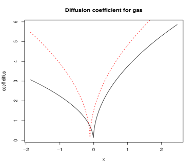
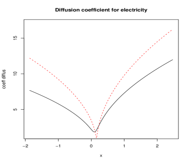
The algorithms converged quickly. The diffusion coefficient functions σj~(.,θj)\tilde{\sigma_{j}}(.,\theta_{j}), j=g,e𝑗𝑔𝑒j=g,e, with the fitted parameters, are documented in Figure 6. We see that the shape of the diffuion coefficients are quite similar for the gas and electricity spot deseasonalized spot prices. Spikes are obtained when the processes Ygsuperscript𝑌𝑔Y^{g} and Yesuperscript𝑌𝑒Y^{e} are far from their mean by clusters of volatility, i.e. periods of high volatility. As we see, large values are more likely and the asymmetry is more pronounced for electricity spot prices than for gas spot prices. We clearly see spikes as cluster of volatility are more probable and more intense for electricity deseasonalized spot prices than for gas deseasonalized spot prices.
Refer to caption
Refer to caption
Figure 6: Squared diffusion coefficients using fitted parameters with maximum likelihood estimation of order 0 (normal lines) and of order 1 (dashed lines).

In order to simulate price trajectories, we consider the Euler-Maruyama schemes defined by (10) and (9). If one is concerned by estimating some quantities (for instance quantiles) on only one trajectory then one should replace the above Euler schemes of Xgsuperscript𝑋𝑔X^{g} and Xesuperscript𝑋𝑒X^{e} with their respective Milstein schemes X~gsuperscript~𝑋𝑔\tilde{X}^{g} and X~esuperscript~𝑋𝑒\tilde{X}^{e} in order to achieve a smaller strong error rate. It consists in devising the following schemes for j=g,e𝑗𝑔𝑒j=g,e,

X~tk+1j=eλj(tk+1tk)(X~tkj+(μjλj12σjσj(X~tkj;θj))Δ)+σj(X¯tkj;θj)1e2λjΔ2λjGk+1j+12σjσj(X~tkj;θj)(Gk+1j)2,X~0j=x0j,formulae-sequencesubscriptsuperscript~𝑋𝑗subscript𝑡𝑘1superscript𝑒subscript𝜆𝑗subscript𝑡𝑘1subscript𝑡𝑘subscriptsuperscript~𝑋𝑗subscript𝑡𝑘subscript𝜇𝑗subscript𝜆𝑗12subscript𝜎𝑗superscriptsubscript𝜎𝑗subscriptsuperscript~𝑋𝑗subscript𝑡𝑘subscript𝜃𝑗Δsubscript𝜎𝑗subscriptsuperscript¯𝑋𝑗subscript𝑡𝑘subscript𝜃𝑗1superscript𝑒2subscript𝜆𝑗Δ2subscript𝜆𝑗subscriptsuperscript𝐺𝑗𝑘112subscript𝜎𝑗superscriptsubscript𝜎𝑗subscriptsuperscript~𝑋𝑗subscript𝑡𝑘subscript𝜃𝑗superscriptsubscriptsuperscript𝐺𝑗𝑘12subscriptsuperscript~𝑋𝑗0subscriptsuperscript𝑥𝑗0\tilde{X}^{j}_{t_{k+1}}=e^{-\lambda_{j}(t_{k+1}-t_{k})}\left(\tilde{X}^{j}_{t_{k}}+\left(\mu_{j}\lambda_{j}-\frac{1}{2}{\sigma_{j}}{\sigma_{j}}^{{}^{\prime}}(\tilde{X}^{j}_{t_{k}};\theta_{j})\right)\Delta\right)\\ +\sigma_{j}\left(\bar{X}^{j}_{t_{k}};\theta_{j}\right)\sqrt{\frac{1-e^{-2\lambda_{j}\Delta}}{2\lambda_{j}}}G^{j}_{k+1}+\frac{1}{2}{\sigma_{j}}{\sigma_{j}}^{{}^{\prime}}(\tilde{X}^{j}_{t_{k}};\theta_{j})\left(G^{j}_{k+1}\right)^{2},\ \tilde{X}^{j}_{0}=x^{j}_{0},

where σjsuperscriptsubscript𝜎𝑗{\sigma_{j}}^{{}^{\prime}} is the first derivative of σjsubscript𝜎𝑗{\sigma_{j}}.

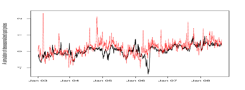
In the following simulations, we consider Milstein schemes of step tk=kΔsubscript𝑡𝑘𝑘Δt_{k}=k\Delta, with Δ=1252Δ1252\Delta=\frac{1}{252}. Next, we add to the simulated processes the two seasonality functions. In Figure 7, the simulated deseasonalized spot prices are represented. We see that both commodities are strongly linked and that the model mimics the statistical behaviour of the deseasonalized spot prices. In Figure 8, the simulated spot prices are represented. In Figure 9, both simulated and historical ACFs and CCF are plotted. We clearly see that the model reproduces the correlation structures.
Refer to caption
Figure 7: A simulation of gas (normal line) and electricity (dotted line) deseasonalized spot prices.
Refer to caption
Refer to caption
Figure 8: Simulated Electricity spot prices on the Powernext market on the left and Gas spot prices at the NBP on the right for the period 14 January 2003 till 20 August 2008.
Refer to caption
(a) ACF of one simulation of Ygsuperscript𝑌𝑔Y^{g}
Refer to caption
(b) ACF of one simulation of Yesuperscript𝑌𝑒Y^{e}
Refer to caption
(c) CCF of the simulations
Figure 9: ACFs and CCF of simulated gas and electricity spot prices (normal lines) with the historical ACFs and CCF (dotted lines).

5.2 Application: measuring risk of a cross-commodity portfolio

In this section, we aim at measuring the risk of a portfolio composed of a short position in a power plant that produces electricity from gas day by day t1<<tNsubscript𝑡1subscript𝑡𝑁t_{1}<\ ...<\ t_{N} for several maturities T=tN= 6𝑇subscript𝑡𝑁6T=t_{N}=\ 6 months, 111 year and 333 years. The loss at time 0 of the portfolio with a time horizon T𝑇T can be written

LT=k=1Nertk(StkehRStkgC)+PTc,subscript𝐿𝑇superscriptsubscript𝑘1𝑁superscript𝑒𝑟subscript𝑡𝑘subscriptsubscriptsuperscript𝑆𝑒subscript𝑡𝑘subscript𝑅subscriptsuperscript𝑆𝑔subscript𝑡𝑘𝐶superscriptsubscript𝑃𝑇𝑐L_{T}=\sum_{k=1}^{N}e^{-rt_{k}}\left(S^{e}_{t_{k}}-h_{R}S^{g}_{t_{k}}-C\right)_{+}-P_{T}^{c},

where r=5%𝑟percent5r=5\% is the annual interest rate, hR=3subscript𝑅3h_{R}=3 denotes the Heat Rate, C=5𝐶5C=5 €/MWh denotes the generation costs and where PTcsuperscriptsubscript𝑃𝑇𝑐P_{T}^{c} is an estimation of the price of the option on the power plant obtained by a crude Monte Carlo simulation, namely

PTck=1Nertk𝐄[(StkehRStkgC)+].superscriptsubscript𝑃𝑇𝑐superscriptsubscript𝑘1𝑁superscript𝑒𝑟subscript𝑡𝑘𝐄delimited-[]subscriptsubscriptsuperscript𝑆𝑒subscript𝑡𝑘subscript𝑅subscriptsuperscript𝑆𝑔subscript𝑡𝑘𝐶P_{T}^{c}\approx\sum_{k=1}^{N}e^{-rt_{k}}\mathbf{E}\left[\left(S^{e}_{t_{k}}-h_{R}S^{g}_{t_{k}}-C\right)_{+}\right].

Since gas and electricity markets are incomplete, we price and estimate risk measures under the historical probability. In order to measure the risk, we consider the Value-at-Risk (VaR), which is certainly the most commonly used risk measures in the context of risk management. By definition, the Value-at-Risk at level α(0,1)𝛼01\alpha\in(0,1) (VaRα) of a given portfolio is the lowest amount not exceeded by its loss with probability α𝛼\alpha. In this example, we set α=95%𝛼percent95\alpha=95\%. Actually, for the considered portfolio, the VaRα is the unique solution ξ𝜉\xi of the equation

𝐏[LTξ]=α.𝐏delimited-[]subscript𝐿𝑇𝜉𝛼\mathbf{P}\left[L_{T}\leq\xi\right]=\alpha.

The portfolio’s VaRα is just a quantile of its loss and is interpreted as a reasonable worst case level.

Now, we are interested in measuring the impact of the proposed model for gas and electricity spot prices on the portfolio’s VaR. In order to do that, we consider three different models:

  • Case 1: the mean-reverting cross-commodity model (in its geometric form) proposed in this paper and defined by (11) and (12). It modelizes typical features of gas and electricity spot prices likes spikes and the long term dependency.

  • Case 2: a slight modification of the previous model in which we do not take into account the dependence of the two energy spot prices. To be more precise, we consider the following model specification

    Sg(t)superscript𝑆𝑔𝑡\displaystyle S^{g}(t) =g(t)×eXg(t)+Zg(t),absent𝑔𝑡superscript𝑒superscript𝑋𝑔𝑡superscript𝑍𝑔𝑡\displaystyle=g(t)\times e^{X^{g}(t)+Z^{g}(t)},
    Se(t)superscript𝑆𝑒𝑡\displaystyle S^{e}(t) =e(t)×eXe(t)+Ze(t),absent𝑒𝑡superscript𝑒superscript𝑋𝑒𝑡superscript𝑍𝑒𝑡\displaystyle=e(t)\times e^{X^{e}(t)+Z^{e}(t)},

    where Xgsuperscript𝑋𝑔X^{g} and Xesuperscript𝑋𝑒X^{e} are solutions of (Eb,σsubscript𝐸𝑏𝜎E_{b,\sigma}) with b𝑏b and σ𝜎\sigma defined in (3), and where Zgsuperscript𝑍𝑔Z^{g}, Zesuperscript𝑍𝑒Z^{e} are two independant Gaussian OU processes solution of (5). By this model, we want to measure the impact on the VaRα of the long term dependency modeling. The calibration process is slightly modified since Sgsuperscript𝑆𝑔S^{g} and Sesuperscript𝑆𝑒S^{e} are now independent. The step 2 is replaced by two different minimizations corresponding to each ACF. Steps 1 and 3 remain unchanged.

  • Case 3: a slight modification of the case 1 in which we do not modelize the spikes feature. To be more precise, we replace the NIG-distributed processes by Gaussian Ornstein-Uhlenbeck processes, namely

    Sg(t)superscript𝑆𝑔𝑡\displaystyle S^{g}(t) =g(t)×eZg(t)+Z(t),absent𝑔𝑡superscript𝑒superscript𝑍𝑔𝑡𝑍𝑡\displaystyle=g(t)\times e^{Z^{g}(t)+Z(t)},
    Se(t)superscript𝑆𝑒𝑡\displaystyle S^{e}(t) =e(t)×eZe(t)+Z(t),absent𝑒𝑡superscript𝑒superscript𝑍𝑒𝑡𝑍𝑡\displaystyle=e(t)\times e^{Z^{e}(t)+Z(t)},

    where Zgsuperscript𝑍𝑔Z^{g}, Zesuperscript𝑍𝑒Z^{e}, Z𝑍Z are three different Gaussian OU processes solution of (5). By this model, we want to quantify the impact on the VaRα of the spike feature of gas and electricity spot prices.

In each case, we estimate PTcsuperscriptsubscript𝑃𝑇𝑐P_{T}^{c} and the VaRα using 10 000 Monte Carlo simulations. We devise Euler schemes of step tk=kΔsubscript𝑡𝑘𝑘Δt_{k}=k\Delta with Δ=1252Δ1252\Delta=\frac{1}{252}. In order to estimate the VaRα, we use the inversion of the simulated empirical distribution function.

Remark 5.1.

Since gas and electricity spot prices are sums of diffusion processes solution of (Eb,σ)subscript𝐸𝑏𝜎\left(E_{b,\sigma}\right), one can easily use the method investigated in [11] to estimate the VaRα and other risk measures. It is based on stochastic approximation algorithms with an adaptive variance reduction tool (unconstrained importance sampling algorithm). The method is known to achieve good variance reduction when α1𝛼1\alpha\approx 1 as it is often the case. For the sake of simplicity, we only considered the classical method based on the inversion of the empirical distribution function.

The results are summarized in Tables 5.2. Note that for each case, the estimations are computed using the same pseudo-random number generator initialized with the same seed. The number in parentheses refers to the 95%percent9595\% confidence level.

Maturity PTcsuperscriptsubscript𝑃𝑇𝑐P_{T}^{c}\;\; (±(\pmError) VaRα𝛼{}_{\alpha}\;
Case 1 (Proposed model) 6 months 83.3 (±plus-or-minus\pm3.3) 262.4
1 year 220.1 (±plus-or-minus\pm5.5) 495.4
3 years 745.0 (±plus-or-minus\pm11.2) 1081.0
Case 2 (No cross-correlation) 6 months 51.2 (±plus-or-minus\pm2.9) 250.1
1 year 222.6 (±plus-or-minus\pm8.4) 880.2
3 years 850.6 (±plus-or-minus\pm21.3) 2213.1
Case 3 (Gaussian model) 6 months 32.9 (±plus-or-minus\pm1.1) 107.7
1 year 129.8 (±plus-or-minus\pm2.7) 275.9
3 years 437.1 (±plus-or-minus\pm5.8) 565.5
Table 1: Estimation of the price of the Power plant and the VaRα of the portfolio.

We observe that there are slight differences in terms of the price PTcsuperscriptsubscript𝑃𝑇𝑐P_{T}^{c} between the case 1 and 2 but huge differences in terms of risk. Taking into account the long term correlation between gas and electricity spot prices can reduce substantially the risk of this portfolio. Modeling independently each energy spot prices leads to an overestimation of the VaRα of the portfolio’s loss. The results obtained by using the model investigated in case 3 shows that introducing the spikes behavior into the model can increase greatly both PTcsuperscriptsubscript𝑃𝑇𝑐P_{T}^{c} and the risk of the portfolio. We also estimated the same quantities using the arithmetic version of the three models presented above. We obviously obtained different values from the ones presented but the same conclusions hold: modeling adequatly the cross correlation between gas and electricity spot prices reduces the risk of portfolio whereas modeling adequatly the spiky behavior of both commodities increases greatly the price of the option and the risk associated to the portfolio.

References

  • [1] A. Azzalini. Maximum likelihood estimation of order m for stationary stochastic processes. Biometrika, 70:381–387, 1983.
  • [2] M. T. Barlow. A diffusion model for electricity prices. Math. Finance, 12(4):287–298, 2002.
  • [3] O. E. Barndorff-Nielsen. Normal inverse Gaussian distributions and stochastic volatility modelling. Scand. J. Statist., 24(1):1–13, 1997.
  • [4] F. Benth, J. Kallsen, and T. Meyer-Brandis. A non-Gaussian Ornstein-Uhlenbeck process for electricity spot price modeling and derivatives pricing. Appl. Math. Finance, 14(2):153–169, 2007.
  • [5] F. Benth and P. Kettler. Dynamic copula models for the spark spread. Technical report, E-print no. 14, Department of Mathematics, University of Oslo, 2006.
  • [6] F. Benth and R. Kufakunesu. Pricing of exotic energy derivatives based on arithmetic spot models. Technical report, 2007.
  • [7] B. Bibby, I. Skovgaard, and M. Sørensen. Diffusion-type models with given marginal distribution and autocorrelation function. Bernoulli, 11(2):191–220, 2005.
  • [8] R. W. Butler. Saddlepoint approximations with applications. Cambridge Series in Statistical and Probabilistic Mathematics. Cambridge University Press, Cambridge, 2007.
  • [9] S. Deng and W. Jiang. Levy process-driven mean-reverting electricity price model: the marginal distribution analysis. Decision Support Systems, 40(3-4):483–494, 2005.
  • [10] O. Elerian. A note on the existence of a closed form conditional transition density for milstein scheme. Working Paper, Nuffield College, Oxford University, 1998.
  • [11] N. Frikha. PhD thesis, Université Pierre et Marie Curie - Gaz de France, In progress.
  • [12] H. Geman. Commodities and commodity derivatives: modeling and pricing for agriculturals, metals and energy. Wiley & Sons, 2005.
  • [13] H. Geman and A. Roncoroni. Understanding the fine structure of electricity prices. The Journal of Business, 79(3):1225–1261, 2006.
  • [14] B. Hambly, S. Howison, and T. Kluge. Modelling spikes and pricing swing options in electricity markets. Quantitative Finance, 9:937–949, 2009.
  • [15] T. Kanamura and K. Ōhashi. A structural model for electricity prices with spikes: Measurement of spike risk and optimal policies for hydropower plant operation. Energy Economics, 29(5):1010–1032, 2007.
  • [16] I. Karatzas and S. Shreve. Brownian motion and stochastic calculus. 2nd ed. Graduate Texts in Mathematics, 113. New York etc.: Springer-Verlag. xxiii, 470 p. DM 68.00/pbk , 1991.
  • [17] S. Karlin and H. Taylor. A second course in stochastic processes. New York etc.: Academic Press, A Subsidiary of Harcourt Brace Jovanovich, Publishers. XVIII, 542 p. $ 35.00 , 1981.
  • [18] M. Kessler. Estimation of an ergodic diffusion from discrete observations. Journal of Statistics, 24:211–229, 1997.
  • [19] D. Madan and M. Yor. Making Markov martingales meet marginals: with explicit constructions. Bernoulli, 8(4):509–536, 2002.
  • [20] T. Meyer-Brandis and P. Tankov. Multi-factor jump-diffusion models of electricity prices. Int. J. Theor. Appl. Finance, 11(5):503–528, 2008.
  • [21] E. Schwartz. The stochastic behavior of commodity prices: Implications for valuation and hedging. Journal of finance, pages 923–973, 1997.
  • [22] P. Villaplana. Pricing power derivatives: A two-factor jump-diffusion approach. Conference Paper, European Finance Association. In 30th Annual Meeting, 2003.